Finite-volume effects in $(g-2)^{\text{HVP,LO}}_{\mu}$

Abstract

An analytic expression is derived for the leading finite-volume effects arising in lattice QCD calculations of the hadronic-vacuum-polarization contribution to the muon’s magnetic moment $a_{\mu}^{\text{HVP,LO}}\equiv(g-2)_{\mu}^{\text{HVP,LO}}/2$. For calculations in a finite spatial volume with periodicity $L$, $a_{\mu}^{\text{HVP,LO}}(L)$ admits a transseries expansion with exponentially suppressed $L$ scaling. Using a Hamiltonian approach, we show that the leading finite-volume correction scales as $\exp[-M_{\pi}L]$ with a prefactor given by the (infinite-volume) Compton amplitude of the pion, integrated with the muon-mass-dependent kernel. To give a complete quantitative expression, we decompose the Compton amplitude into the space-like pion form factor, $F_{\pi}(Q^{2})$, and a multi-particle piece. We determine the latter through NLO in chiral perturbation theory and find that it contributes negligibly and through a universal term that depends only on the pion decay constant, with all additional low-energy constants dropping out of the integral.

I Introduction

The discrepancy between experimental Bennett et al. (2004, 2006) and theoretical Jegerlehner and Nyffeler (2009); Davier et al. (2017); Keshavarzi et al. (2018) values and the ongoing measurements at Fermilab Carey et al. (2009); Grange et al. (2015); Flay (2017); Hong (2018) and J-PARC Shimomura (2015); Sato (2017) have motivated various lattice QCD (LQCD) collaborations to calculate the hadronic contributions to $(g-2)_{\mu}$, which currently dominate the theoretical uncertainty Blum (2003); Burger et al. (2014); Chakraborty et al. (2014, 2016); Blum et al. (2016a, 2017); Chakraborty et al. (2017); Blum et al. (2016b); Della Morte et al. (2017); Giusti et al. (2017); Borsanyi et al. (2018); Giusti et al. (2018a); Asmussen et al. (2018); Giusti et al. (2018b); Blum et al. (2018); Davies et al. (2019); Gérardin et al. (2019). The relevant contributions divide into hadronic light-by-light, leading-order hadronic vacuum polarization (LO HVP) and electromagnetic as well as strong-isospin corrections to the HVP. As the dominant hadronic contribution, the LO HVP must be determined with sub-percent uncertainties to reach a total theory uncertainty competitive with the expected experimental precision Jegerlehner (2018). Depending on the central values of the theoretical and experimental updates, the improved precision on both sides will provide powerful constraints on, or else strong evidence for, new-physics beyond the Standard Model.

As the only known, systematically-improvable approach to non-perturbative QCD, numerical lattice QCD is a natural tool in the determination of the LO HVP where a systematic and precise value is of great importance. The most common approach is to estimate $a_{\mu}^{\text{HVP,LO}}\equiv(g-2)_{\mu}^{\text{HVP,LO}}/2$ via the integral Bernecker and Meyer (2011)

$$a_{\mu}^{\text{HVP,LO}}(T,L)=\frac{2\alpha^{2}}{m_{\mu}^{2}}\int_{0}^{T/2}dx_{0}\,\widehat{\mathcal{K}}(m_{\mu}x_{0})G_{T,L}(x_{0})\,,$$ (1)

where $\alpha\approx 1/137$ is the fine-structure constant, $m_{\mu}$ the muon mass and

$$G_{T,L}(x_{0}) \equiv-\frac{1}{3}\sum_{k=1}^{3}\int_{L^{3}}\!d^{3}\boldsymbol{x}\,\langle j_{k}(x_{0},\boldsymbol{x})j_{k}(0)\rangle_{T,L}\,,$$ (2)

$$\begin{split}\widehat{\mathcal{K}}(t)&\equiv t^{2}-2\pi t+(8\gamma_{E}-2)+\frac{4}{t^{2}}+8\log(t)\\[-3.0pt] &\hskip 30.0pt-\frac{8K_{1}(2t)}{t}-8\int_{0}^{\infty}dv\frac{e^{-t\sqrt{v^{2}+4}}}{(v^{2}+4)^{3/2}}\,.\end{split}$$ (3)

Here $j_{\mu}(x)=\sum_{f}q_{f}\overline{\psi}_{f}(x)\gamma_{\mu}\psi_{f}(x)$ is the Euclidean-signature vector current and $K_{1}(z)$ a Bessel function. We have used notation to emphasize that the calculation is performed in a finite-volume $T\times L^{3}$ Euclidean spacetime with periodic geometry.

In Eq. (1) the finite temporal extent is accommodated by cutting the integral at $T/2$. We leave a detailed analysis of finite-$T$ effects, arising both from the boundary conditions and the treatment of large $x_{0}$ in the integral, to a future work. In this work we consider only the finite-$L$ effects, defining $a_{\mu}^{\text{HVP,LO}}(L)\equiv\lim_{T\to\infty}a_{\mu}^{\text{HVP,LO}}(T,L)$. We will show that this quantity has only exponentially-suppressed finite-volume effects, and the suppression is controlled by the pion mass $M_{\pi}$.

Even when $T$ is taken very large, the large-$x_{0}$ region of the integral in Eq. (1) cannot be calculated from the measured two-point function because of the well-known exponential degradation of the signal-to-noise ratio. In practice, one can calculate the two-point function $G_{T\to\infty,L}(x_{0})$ for $x_{0}<\tau_{\text{c}}$ from numerical simulations (possibly with a mild extrapolation to saturate the $T\to\infty$ limit), and then use additional inputs to reconstruct the $x_{0}>\tau_{\text{c}}$ region. This yields a decomposition

$$a_{\mu}^{\text{recon}}(L)=a_{\mu}(L|x_{0}<\tau_{\text{c}})+a^{\text{recon}}_{\mu}(L|x_{0}>\tau_{\text{c}})\,,$$ (4)

where the superscript “recon” stands for reconstructed. The first term is calculated by restricting the integration domain in Eq. (1) to $0<x_{0}<\tau_{\text{c}}$ and by using the measured two-point function. The second term is obtained from an analogous formula where the integral is taken over $\tau_{\text{c}}<x_{0}<\infty$ and the reconstructed two-point function is used.

We will see that $a_{\mu}(L|x_{0}<\tau_{\text{c}})$ approaches the infinite-volume limit exponentially fast. On the other hand, $a^{\text{recon}}_{\mu}(L|x_{0}>\tau_{\text{c}})$ may approach $L\to\infty$ more slowly, depending on the exact prescription used. As an extreme example, if one estimates $G_{\infty,L}(x_{0})$ for $x_{0}>\tau_{\text{c}}$ by summing over a fixed number of finite-volume states, the resulting contribution to the HVP will have power-law $L$-dependence Lüscher (1986a); Lellouch and Lüscher (2001). In practice more sophisticated procedures are employed and the resulting scaling must be considered on a case by case basis.

Our main result, the formula for the leading $\exp[-M_{\pi}L]$ finite-volume effect to $a_{\mu}^{\text{HVP,LO}}(L)$, is presented in Sec. II, and is derived in Sec. III by means of a hamiltonian formalism in which quantization along a spatial direction is used to pick out the complete functional form non-perturbatively. In Sec. IV we discuss the implications of our expression for ongoing calculations. We find that the dominant contribution enters through the space-like pion form factor, and, since the latter is readily calculated on the lattice, this provides a viable method for correcting the leading $L$-dependence. We estimate also the dominant contribution to the finite-volume effects of $a_{\mu}(L|x_{0}<\tau_{\text{c}})$, which can be useful information when devising a strategy along the lines of Eq. (4).

Our results differ from Refs. Aubin et al. (2016); Bijnens and Relefors (2017) in that these work to a fixed order in chiral perturbation theory (ChPT) whereas our result is the full non-perturbative expression, to leading-order in the large $L$ expansion. In this regard it is worth emphasizing that the strict chiral expansion is limited by the fact that, at N³LO, the momentum-space vector correlator receives a $Q^{6}$ contribution that leads to a divergence in the integral defining $a_{\mu}^{\text{HVP,LO}}$.

II Result

We define

$$\Delta a_{\mu}(L)\equiv a_{\mu}^{\text{HVP,LO}}(L)-\lim_{L\to\infty}a_{\mu}^{\text{HVP,LO}}(L)\,,$$ (5)

where, as in the introduction, we ignore the effects of the finite temporal extent. These scale as $e^{-M_{\pi}T}$ and $e^{-M_{\pi}\sqrt{T^{2}+L^{2}}}$. Therefore in the commonly used setup $T=2L$, the finite-$T$ corrections are sub-leading and should be dropped. The separation is plausible from the perspective of a generic effective field theory. Volume effects can be encoded via position-space propagators, summed over all periodic images. The propagator’s form then leads to exponential decay falling according to the image distance multiplied with the pion mass. The detailed proof of this separation, based on the methods of Ref. Lüscher (1986b), is given in a second longer publication.

In Sec. III we show that the leading finite-$L$ corrections are given by

$$\Delta a_{\mu}(L)=-\frac{2\alpha^{2}}{m_{\mu}^{2}}\int\frac{dp_{3}}{2\pi}\frac{e^{-L\sqrt{M_{\pi}^{2}+p_{3}^{2}}}}{4\pi L}\int_{0}^{\infty}dx_{0}\,\widehat{\mathcal{K}}(m_{\mu}x_{0})\int\frac{dk_{3}}{2\pi}\cos(x_{0}k_{3})\!\!\sum_{q=0,\pm 1}\text{Re}\,T_{q}(-k_{3}^{2},-k_{3}p_{3})+\mathcal{O}(e^{-\sqrt{2}M_{\pi}L})\,,$$ (6)

where $T_{q}$ is the Compton amplitude

$$T_{q}(k^{2},k\cdot p)\equiv\\ i\lim_{\boldsymbol{p}^{\prime}\to\boldsymbol{p}}\int d^{4}x\,e^{ikx}\langle\boldsymbol{p}^{\prime},q|\text{T}\mathcal{J}_{\rho}(x)\mathcal{J}^{\rho}(0)|\boldsymbol{p},q\rangle_{\infty}\,,$$ (7)

in the forward limit. Here $|\boldsymbol{p},q\rangle$ is the relativistically-normalized state of a single pion with momentum $\boldsymbol{p}$ and charge $q$, $k^{2}=k_{0}^{2}-\boldsymbol{k}^{2}$ and $k\cdot p=k_{0}p_{0}-\boldsymbol{k}\boldsymbol{p}$ are the Minkowski squared norm and scalar product. Following the discussion after Eq. (5), the subleading exponential, $e^{-\sqrt{2}M_{\pi}L}$, arisies from an image displaced in two of the spatial directions.

$\mathcal{J}_{\mu}(x)$ is the Minkowski current. In the Schrödinger picture this is related to its Euclidean counterpart via

$$\mathcal{J}_{0}(\boldsymbol{x})=j_{0}(\boldsymbol{x})\ ,\qquad\mathcal{J}_{k}(\boldsymbol{x})=-ij_{k}(\boldsymbol{x})\,,$$ (8)

and the corresponding Heisenberg operators are

$$j_{\mu}(x_{0},\boldsymbol{x})=e^{x_{0}H}j_{\mu}(\boldsymbol{x})e^{-x_{0}H}\ ,$$ (9)

$$\mathcal{J}_{\mu}(t,\boldsymbol{x})=e^{itH}\mathcal{J}_{\mu}(\boldsymbol{x})e^{-itH}\ .$$ (10)

III Derivation

Define $G_{L_{\rho}}(x_{0})$ exactly as $G_{T,L}(x_{0})$ in Eq. (2) but in a volume in which all four directions may differ, i.e. with $L_{0}\times L_{1}\times L_{2}\times L_{3}$. Then introduce $\Delta G_{3}(x_{0}|L)\equiv[1-\lim_{L_{0,1,2}\to\infty}]G_{L_{\rho}}(x_{0})$ as the finite-volume residue due to compactification in the $3$ direction only.

To determine $\Delta G_{3}(x_{0}|L)$, we study $G_{L_{\rho}}(x_{0})$ with geometry $L_{\rho}=(L_{\perp},L_{\perp},L_{\perp},L)$ and quantize along the 3 direction. Defining $\underline{x}=(x_{1},x_{2},x_{0})=(x_{\perp},x_{0})$, the Hamiltonian representation of the Euclidean two-point function yields

$$G_{L_{\rho}}(x_{0})=-\frac{1}{3}\int_{0}^{L_{\perp}}d^{2}x_{\perp}\int_{0}^{L}dx_{3}\\ \times\frac{\mathrm{tr}\,[e^{-(L-x_{3})H}j_{\mu}(\underline{x})e^{-x_{3}H}j_{\mu}(\underline{0})]}{\mathrm{tr}\,e^{-LH}}\ ,$$ (11)

where the Hamiltonian has a discrete finite-volume spectrum of states in $L_{\perp}^{3}$ and the trace is taken over this Hilbert space. Here we are using $L_{\bot}$ to ensure that intermediate expressions are well-defined. This will be sent to infinity at the end of the calculation. For simplicity, in this formula we have assumed periodic boundary conditions for gluons and antiperiodic boundary conditions for fermions in the $3$ direction. To account for the commonly-used periodic boundary contitions for fermions one should introduce $(-1)^{F}$ in all traces, where $F$ is the fermion number. This does not change the leading exponential contribution, since this is due to single-pion, hence bosonic, states.

Let $|n\rangle$ be a basis of simultaneous eigenstates of the Hamiltonian (eigenvalue $E_{n}$), the momentum (eigenvalue $\boldsymbol{p}_{n}$), the charge (eigenvalue $q_{n}$) operators. Inserting a complete set of such states in both the numerator and the denominator then gives

$$G_{L_{\rho}}(x_{0})=-\frac{1}{3}\sum_{n,n^{\prime}}\frac{e^{-LE_{n}}}{\sum_{n^{\prime\prime}}e^{-LE_{n^{\prime\prime}}}}\int_{0}^{L_{\perp}}d^{2}x_{\perp}\int_{0}^{L}dx_{3}\\ \times e^{-x_{3}(E_{n^{\prime}}-E_{n})}\langle n|j_{\mu}(\underline{x})|n^{\prime}\rangle\langle n^{\prime}|j_{\mu}(\underline{0})|n\rangle\ .$$ (12)

The role of the coordinates $x_{0}$ and $x_{3}$ in this analysis is potentially confusing. In our final results $x_{0}$ plays the role of the time coordinate. This is the coordinate of integration in Eq. (1), typically parametrizing the longest Euclidean direction. Here, to identify the leading $L$-dependence, it is convenient to quantize along the $3$ direction. One must only take care that, in any given expression, all energies and all states are consistently defined with respect to the same quantization direction.

Returning to Eq. (12), the integral over $x_{3}$ can be calculated explicitly. To avoid the need of separating $E_{n^{\prime}}=E_{n}$ terms from the rest, we introduce the following identity, which holds for all values of $E_{n}$, $E_{n^{\prime}}$

$$e^{-LE_{n}}\int_{0}^{L}dx_{3}\ e^{-x_{3}(E_{n^{\prime}}-E_{n})}=\\ \lim_{\epsilon\to 0^{+}}\text{Re}\frac{e^{-L(E_{n}+i\epsilon)}-e^{-L(E_{n^{\prime}}-i\epsilon)}}{E_{n^{\prime}}-E_{n}-2i\epsilon}\,.$$ (13)

Substituting into Eq. (12) and exchanging $n^{\prime}\leftrightarrow n$ in certain terms, we obtain

$$G_{L_{\rho}}(x_{0})=-\frac{1}{3}\lim_{\epsilon\to 0^{+}}\sum_{n}\frac{e^{-LE_{n}}}{\sum_{n^{\prime\prime}}e^{-LE_{n^{\prime\prime}}}}\int_{0}^{L_{\perp}}d^{2}x_{\perp}\\ \times\left\{\text{Re}\langle n|j_{\mu}(\underline{x})\frac{e^{-iL\epsilon}}{H-E_{n}-2i\epsilon}j_{\mu}(\underline{0})|n\rangle+(\epsilon\to-\epsilon)\right\}\ .$$ (14)

This expectation value can be expressed in terms of the (finite-volume) Minkowskian two-point function via

$$\text{Re}\langle n|j_{\mu}(\underline{x})\frac{e^{-iL\epsilon}}{H-E_{n}-2i\epsilon}j_{\mu}(\underline{0})|n\rangle+(\epsilon\to-\epsilon)=\\ \text{Re}\,ie^{-iL\epsilon}\int_{-\infty}^{\infty}dt\ e^{-2\epsilon|t|}\langle n|\text{T}\mathcal{J}_{\mu}(t,\underline{x})\mathcal{J}^{\mu}(0)|n\rangle\ ,$$ (15)

which is valid for $\epsilon>0$ and can be easily proven using Eq. (10) and integrating over $t$ explicitly. We stress that this is a mathematical identity and the parameter $t$ has no relation to any of the spacetime coordinates in the system.

The expansion about $L\to\infty$ is now straightforward as the exponentials are manifest and one can identify the relevant contribution. Neglecting terms of order $e^{-2M_{\pi}L}$ we reach

$$\Delta G_{3}(x_{0}|L)=-\frac{1}{3}\lim_{\epsilon\to 0^{+}}\sum_{M_{\pi}\leq E_{n}<2M_{\pi}}e^{-LE_{n}}\int_{0}^{L_{\perp}}d^{2}x_{\perp}\\ \times\text{Re}\,ie^{-iL\epsilon}\int_{-\infty}^{\infty}dt\ e^{-2\epsilon|t|}\langle n|\text{T}\mathcal{J}_{\mu}(t,\underline{x})\mathcal{J}^{\mu}(0)|n\rangle_{\text{c}}\ ,$$ (16)

where the connected expectation value is defined as $\langle n|\mathcal{O}|n\rangle_{\text{c}}\equiv\langle n|\mathcal{O}|n\rangle-\langle 0|\mathcal{O}|0\rangle$. At this point we can take the $L_{\perp}\to\infty$ limit. This is done by replacing the sum over the states in the one-particle region with the phase-space integral

$$\sum_{M_{\pi}\leq E_{n}<2M_{\pi}}e^{-LE_{n}}|n\rangle\langle n|\ \ \ \underset{L_{\bot}\to\infty}{\longrightarrow}\\ \sum_{q=0,\pm 1}\int_{E(\boldsymbol{p})<2M_{\pi}}\!\frac{d^{3}\boldsymbol{p}}{(2\pi)^{3}}\frac{e^{-LE(\boldsymbol{p})}}{2E(\boldsymbol{p})}|\boldsymbol{p},q\rangle\langle\boldsymbol{p},q|\ ,$$ (17)

and by replacing the connected expectation value with the forward limit

$$i\langle n|\text{T}\mathcal{J}_{\mu}(t,\underline{x})\mathcal{J}^{\mu}(0)|n\rangle_{\text{c}}\to\\ \int\frac{d^{4}k}{(2\pi)^{4}}\,e^{-i(k_{0}t-k_{\perp}x_{\perp}-k_{3}x_{0})}T_{q}(k^{2},k\cdot p)\ ,$$ (18)

where the definition (7) has been used. In the $L_{\perp}\to\infty$ limit, the integrals over $t$ and $x_{\perp}$ are readily calculated, yielding delta functions in $k_{0}=k_{\perp}=0$, i.e.

$$\Delta G_{3}(x_{0}|L)=-\frac{1}{3}\sum_{q=0,\pm 1}\int_{E(\boldsymbol{p})<2M_{\pi}}\!\frac{d^{3}\boldsymbol{p}}{(2\pi)^{3}}\frac{e^{-LE(\boldsymbol{p})}}{2E(\boldsymbol{p})}\\ \times\text{Re}\int\frac{dk_{3}}{2\pi}e^{ik_{3}x_{0}}T_{q}(-k_{3}^{2},-k_{3}p_{3})\ .$$ (19)

In the final expression note that any contribution to the integrand that is odd in $k_{3},p_{3}\to-k_{3},-p_{3}$ must integrate to zero, which justifies the replacement $e^{ik_{3}x_{0}}\to\cos(k_{3}x_{0})$. To complete the derivation we note that the restriction $E(\boldsymbol{p})<2M_{\pi}$ can be dropped, as this amounts to an error of the same order as terms that we are neglecting. Finally, the integral over $p_{\perp}$ can be explicitly calculated. We reach

$$\Delta G_{3}(x_{0}|L)=-\frac{1}{3}\sum_{q=0,\pm 1}\int\!\frac{dp_{3}}{2\pi}\frac{e^{-L\sqrt{M_{\pi}^{2}+p_{3}^{2}}}}{4\pi L}\\ \times\int\frac{dk_{3}}{2\pi}\cos(k_{3}x_{0})\text{Re}T_{q}(-k_{3}^{2},-k_{3}p_{3})\ .$$ (20)

Multiplying the result by $3$ to account for the three directions with compactification $L$, we conclude Eq. (6).

We close by commenting on different choices of boundary conditions. If fermions satisfy $e^{i\theta}$-periodic boundary conditions Bedaque (2004); de Divitiis et al. (2004), i.e. $\psi_{f}(x+L_{\rho}\hat{\rho})=e^{i\theta_{\rho}^{f}}\psi_{f}(x)$, Eq. (11) should be modified by inserting $(-1)^{F}e^{i\sum_{f}\theta_{3}^{f}N_{f}}$ in all traces, where $N_{f}$ is the number operator for the flavour $f$. In this case, Eq. (6) is modified by replacing

$$3\sum_{q=0,\pm 1}\text{Re}T_{q}\to\sum_{k=1}^{3}\{2\cos(\theta_{k}^{u}-\theta_{k}^{d})\text{Re}T_{\pm 1}+\text{Re}T_{0}\}\ ,$$ (21)

where we have used $T_{+1}=T_{-1}\equiv T_{\pm 1}$ as follows from charge-conjugation invariance.

IV Implications

Having derived the leading-order functional form of $\Delta a_{\mu}(L)$, we close by considering the implications for ongoing numerical LQCD calculations. Here we mainly focus on periodic boundary conditions but comment again on the role of twisting below. For convenience we define the charge-summed Compton amplitude, $T\equiv\sum_{q}T_{q}$.

We begin by rewriting Eq. (6) as

$$\Delta a_{\mu}(L) =-\frac{2\alpha^{2}m_{\mu}}{\pi L}\int_{0}^{\infty}dk_{3}\ \hat{g}(k_{3}/m_{\mu})\mathcal{T}^{\prime\prime}(k_{3}^{2}|L)\,,$$ (22)

where we have introduced

$$\mathcal{T}(k_{3}^{2}|L)\equiv\int_{-\infty}^{\infty}\frac{dp_{3}}{2\pi}\ e^{-L\sqrt{M_{\pi}^{2}+p_{3}^{2}}}\,\text{Re}T(-k_{3}^{2},-p_{3}k_{3})\,,$$ (23)

$$\hat{g}(\omega)\equiv\omega\int_{\omega^{2}}^{\infty}\!dy\ \int_{y}^{\infty}\!\frac{dx}{x^{3/2}}\frac{16}{\sqrt{x+4}\,\big{(}\sqrt{x+4}+\sqrt{x}\big{)}^{4}}\,,$$ (24)

and $\mathcal{T}^{\prime\prime}$ is the second derivative of $\mathcal{T}$ with respect to $k_{3}^{2}$.

$-10^{2}\times\Delta a_{\mu}(L)/a_{\mu}^{\text{HVP,LO}}$
$M_{\pi}L$	$F_{\pi}(Q^{2})=1$	$F_{\pi}(Q^{2})=\frac{1}{1+Q^{2}/M^{2}}$	$\mathcal{T}^{\text{reg}}$
4.0	0.639	1.26	$0.019$
5.0	0.579	0.852	$0.005$
6.0	0.348	0.461	$0.001$
7.0	0.180	0.226	$|\cdots|<10^{-3}$
8.0	0.0863	0.104	$|\cdots|<10^{-3}$

Table 1: Contribution to $\Delta a_{\mu}(L)$ from the $F_{\pi}(Q^{2})$-term for functional forms as indicated. Here we take $m_{\mu}/M_{\pi}=106/137$ and $M/M_{\pi}=727/137$. As a reference value we take $a_{\mu}^{\text{HVP,LO}}=700\times 10^{-10}$.

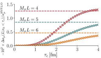
Figure 1: Plot of the $F_{\pi}(Q^{2})$-contribution to $\Delta a_{\mu}(L|x_{0}<\tau_{\text{c}})$ vs. $\tau_{\text{c}}$, taking the monopole ansatz as in Table 1 and $M_{\pi}=M_{\pi}^{\text{phys}}$, for various values of $M_{\pi}L$. The horizontal lines give $\tau_{\text{c}}=\infty$, i.e. the full value for $\Delta a_{\mu}(L)$.

We next decompose the Compton amplitude into its pole and analytical contributions

$$T(k^{2},k\cdot p)\equiv T^{\text{reg}}(k^{2},k\cdot p)\\ +\bigg{[}\frac{2(4M_{\pi}^{2}-k^{2})F_{\pi}^{2}(-k^{2})}{-k^{2}-2p\cdot k-i\epsilon}+(p\to-p)\bigg{]}\,,$$ (25)

where $F_{\pi}$ is the space-like pion form factor and the separation defines $T^{\text{reg}}$. This implies

$$\mathcal{T}(k_{3}^{2}|L)=2(4M_{\pi}^{2}+k_{3}^{2})F_{\pi}^{2}(k_{3}^{2})\zeta(k_{3}^{2}|L)+\mathcal{T}^{\text{reg}}(k_{3}^{2}|L)\,,$$ (26)

where we have introduced

$$\zeta(k_{3}^{2}|L)\equiv 2\text{Re}\int_{-\infty}^{\infty}\frac{dp_{3}}{2\pi}\ \frac{e^{-L\sqrt{M_{\pi}^{2}+p_{3}^{2}}}}{k_{3}^{2}+2p_{3}k_{3}-i\epsilon}\,,$$ (27)

which can be readily reduced to forms well suited to numerical evaluation. The second term in Eq. (26) is given by Eq. (23) with $T\to T^{\text{reg}}$.

In Table 1 we numerically estimate the contribution of the $F_{\pi}(Q^{2})$-dependent term to $\Delta a_{\mu}(L)$, using two functional forms for the specelike form-factor. We have confirmed that the $F_{\pi}(Q^{2})=1$ values match the prediction from ChPT. The monopole form, taken from Ref. Brommel et al. (2007), is known to describe both experimental and lattice data very well up to $Q^{2}=2.45\text{GeV}^{2}$.

We have also calculated the NLO ChPT prediction for $T^{\text{reg}}$ (summed over $\pi_{0}$ and $\pi^{\pm}$ external states),

$$T^{\text{reg}}(-Q^{2},k\cdot p)=c_{0}+c_{1}Q^{2}\\ +\frac{(7M_{\pi}^{2}+4Q^{2})}{6\pi^{2}f_{\pi}^{2}}\ z\,\coth^{-1}z\bigg{|}_{z=\sqrt{1+4M_{\pi}^{2}/Q^{2}}}\,,$$ (28)

with the convention that $f_{\pi}\approx 132\text{MeV}$. The coefficients $c_{0}$ and $c_{1}$ depend on various low-energy constants and on the pion mass. However, the contribution from these terms to $\Delta a_{\mu}(L)$ is identically zero, as can be seen explicitly from Eq. (22). Evaluating the remaining piece, we find that this contributes negligibly as shown in the third column of Table 1. Note that, as can be seen from Eq. (21), using twisted boundary conditions with $\theta_{k}^{u}-\theta_{k}^{d}=\pi/2$ sets the $F_{\pi}(Q^{2})$-dependent piece identically to zero, leaving only the contribution from the neutral pion in $T^{\text{reg}}$. This dramatically reduces the leading $L$-dependence.

$-10^{2}\times\Delta a_{\mu}(L|x_{0}<\tau_{\text{c}})/a_{\mu}^{\text{HVP,LO}}$
$M_{\pi}=M_{\pi}^{\text{phys}}$
$M_{\pi}L$	$\tau_{\text{c}}=1\,\text{fm}$	$1.5\,\text{fm}$	$2\,\text{fm}$	$2.5\,\text{fm}$	$\infty$
4.0	0.0611	0.250	0.550	0.864	1.26
5.0	0.0198	0.0896	0.220	0.385	0.851
6.0	0.00649	0.0313	0.0825	0.155	0.461
7.0	0.00214	0.0108	0.0300	0.0593	0.226
8.0	0.00072	0.00374	0.0108	0.0221	0.104

$M_{\pi}=2M_{\pi}^{\text{phys}}$
$M_{\pi}L$	$\tau_{\text{c}}=1\,\text{fm}$	$1.5\,\text{fm}$	$2\,\text{fm}$	$2.5\,\text{fm}$	$\infty$
4.0	0.231	0.682	1.08	1.28	1.38
5.0	0.0808	0.264	0.456	0.578	0.662
6.0	0.0281	0.0996	0.185	0.247	0.302
7.0	0.00975	0.0369	0.0727	0.102	0.134
8.0	0.00339	0.0135	0.0280	0.0411	0.0576

$M_{\pi}=3M_{\pi}^{\text{phys}}$
$M_{\pi}L$	$\tau_{\text{c}}=1\,\text{fm}$	$1.5\,\text{fm}$	$2\,\text{fm}$	$2.5\,\text{fm}$	$\infty$
4.0	0.455	1.14	1.61	1.82	1.92
5.0	0.162	0.430	0.634	0.730	0.778
6.0	0.0574	0.162	0.249	0.293	0.316
7.0	0.0204	0.0609	0.0970	0.117	0.128
8.0	0.00724	0.0227	0.0376	0.0462	0.0515

Table 2: Tabulated values of the $F_{\pi}(Q^{2})$-contribution to $\Delta a_{\mu}(L|x_{0}<\tau_{\text{c}})$ for various $M_{\pi}L$, $M_{\pi}$ and $\tau_{\text{c}}$. We vary the monople mass according to the result of Ref. Brommel et al. (2007): $M^{2}=0.517(23)\text{GeV}^{2}+0.647(30)M_{\pi}^{2}$ and hold the reference value fixed at $a_{\mu}^{\text{HVP,LO}}=700\times 10^{-10}$.

When separating the $x_{0}$ regions as in Eq. (4), it is useful to identify the cut value, $\tau_{\text{c}}$, which minimizes the the systematic errors given by the finite-volume effects of $a_{\mu}(L|x_{0}<\tau_{\text{c}})$, plus the uncertainties (finite-volume or otherwise) entering through $a^{\text{recon}}_{\mu}(L|x_{0}>\tau_{\text{c}})$. In Fig. 1 we plot the leading finite-$L$ correction of $a_{\mu}(L|x_{0}<\tau_{\text{c}})$ vs $\tau_{\text{c}}$ for various $M_{\pi}L$.

The same data is presented in Table 2, where we additionally vary the pion mass. At constant $M_{\pi}L$, increasing the pion mass leads to a decrease in $m_{\mu}L$ that translates into significantly enhanced volume effects. This behavior is predicted by an asymptotic expansion in $m_{\mu}L$ but the latter exhibits poor convergence so that the dependence is not obvious for these values. Nonetheless the enhancement is clearly realized in these results, with a contribution of $\sim 2\%$ for $\Delta a_{\mu}(L)$ ($\tau_{\text{c}}\to\infty$) with $M_{\pi}L=4$ and $M_{\pi}/M_{\pi}^{\text{phys}}=3$.

V Conclusions

We have presented a fully non-perturbative analysis of the leading finite-$L$ effects in $a_{\mu}^{\text{HVP,LO}}$. In particular, Eq. (6) relates the leading exponential, $\exp[-M_{\pi}L]$, to the Compton amplitude of an off-shell photon scattering against a pion in the forward limit. We also argue that the contribution coming from the one-pion exchange in the Compton amplitude (corresponding to the two-pion exchange in $a_{\mu}^{\text{HVP,LO}}$) is the dominant contribution. We estimate the effect quantitatively using models for the electromagnetic space-like pion form factor.

The results presented here provide an additional tool for systematically removing the finite-$L$ effects in $a_{\mu}^{\text{HVP,LO}}$. One option is to directly improve the result on each ensemble with a dedicated measurement of $F_{\pi}(Q^{2})$. A limitation of this analysis is that the neglected $\exp[-\sqrt{2}M_{\pi}L]$ terms may not be small. As argued in Della Morte et al. (2017) this is certainly true in the case of free pions with $M_{\pi}L\approx 4$ with leading-exponential domination setting in around $M_{\pi}L\approx 6$. In this vein we also stress that our full, non-perturbative result for the leading exponential can be used to assess and improve predictions, e.g. from ChPT, by correcting the leading exponential while keeping the fixed-order prediction for the higher exponentials in the series. This is well-motivated since the structure of the pions becomes less important as the exponentials become more suppressed.

On a technical note, it will be interesting to pursue the Hamiltonian method (already used in Lucini et al. (2016)) for identifying finite-$L$ effects in other contexts.

Acknowledgments

The authors would like to acknowledge and thank Mattia Bruno, Martin Lüscher, Harvey Meyer, and Nazario Tantalo for useful discussions and for helpful comments on a previous version of this manuscript.

References

- Bennett et al. (2004) G. W. Bennett et al. (Muon g-2), Phys. Rev. Lett. 92, 161802 (2004), eprint hep-ex/0401008.
- Bennett et al. (2006) G. W. Bennett et al. (Muon g-2), Phys. Rev. D73, 072003 (2006), eprint hep-ex/0602035.
- Jegerlehner and Nyffeler (2009) F. Jegerlehner and A. Nyffeler, Phys. Rept. 477, 1 (2009), eprint 0902.3360.
- Davier et al. (2017) M. Davier, A. Hoecker, B. Malaescu, and Z. Zhang, Eur. Phys. J. C77, 827 (2017), eprint 1706.09436.
- Keshavarzi et al. (2018) A. Keshavarzi, D. Nomura, and T. Teubner, Phys. Rev. D97, 114025 (2018), eprint 1802.02995.
- Carey et al. (2009) R. M. Carey et al. (2009).
- Grange et al. (2015) J. Grange et al. (Muon g-2) (2015), eprint 1501.06858.
- Flay (2017) D. Flay (Muon g-2), PoS ICHEP2016, 1075 (2017).
- Hong (2018) R. Hong (Muon g-2), in 13th Conference on the Intersections of Particle and Nuclear Physics (CIPANP 2018) Palm Springs, California, USA, May 29-June 3, 2018 (2018), eprint 1810.03729, URL http://lss.fnal.gov/archive/2018/conf/fermilab-conf-18-551-e.pdf.
- Shimomura (2015) K. Shimomura, Hyperfine Interact. 233, 89 (2015).
- Sato (2017) Y. Sato (E34), PoS KMI2017, 006 (2017).
- Blum (2003) T. Blum, Phys. Rev. Lett. 91, 052001 (2003), eprint hep-lat/0212018.
- Burger et al. (2014) F. Burger, X. Feng, G. Hotzel, K. Jansen, M. Petschlies, and D. B. Renner (ETM), JHEP 02, 099 (2014), eprint 1308.4327.
- Chakraborty et al. (2014) B. Chakraborty, C. T. H. Davies, G. C. Donald, R. J. Dowdall, J. Koponen, G. P. Lepage, and T. Teubner (HPQCD), Phys. Rev. D89, 114501 (2014), eprint 1403.1778.
- Chakraborty et al. (2016) B. Chakraborty, C. T. H. Davies, J. Koponen, G. P. Lepage, M. J. Peardon, and S. M. Ryan, Phys. Rev. D93, 074509 (2016), eprint 1512.03270.
- Blum et al. (2016a) T. Blum, P. A. Boyle, T. Izubuchi, L. Jin, A. Jüttner, C. Lehner, K. Maltman, M. Marinkovic, A. Portelli, and M. Spraggs, Phys. Rev. Lett. 116, 232002 (2016a), eprint 1512.09054.
- Blum et al. (2017) T. Blum, N. Christ, M. Hayakawa, T. Izubuchi, L. Jin, C. Jung, and C. Lehner, Phys. Rev. Lett. 118, 022005 (2017), eprint 1610.04603.
- Chakraborty et al. (2017) B. Chakraborty, C. T. H. Davies, P. G. de Oliviera, J. Koponen, G. P. Lepage, and R. S. Van de Water, Phys. Rev. D96, 034516 (2017), eprint 1601.03071.
- Blum et al. (2016b) T. Blum et al. (RBC/UKQCD), JHEP 04, 063 (2016b), [Erratum: JHEP05,034(2017)], eprint 1602.01767.
- Della Morte et al. (2017) M. Della Morte, A. Francis, V. Gülpers, G. Herdoíza, G. von Hippel, H. Horch, B. Jäger, H. B. Meyer, A. Nyffeler, and H. Wittig, JHEP 10, 020 (2017), eprint 1705.01775.
- Giusti et al. (2017) D. Giusti, V. Lubicz, G. Martinelli, F. Sanfilippo, and S. Simula, JHEP 10, 157 (2017), eprint 1707.03019.
- Borsanyi et al. (2018) S. Borsanyi et al. (Budapest-Marseille-Wuppertal), Phys. Rev. Lett. 121, 022002 (2018), eprint 1711.04980.
- Giusti et al. (2018a) D. Giusti, F. Sanfilippo, and S. Simula, Phys. Rev. D98, 114504 (2018a), eprint 1808.00887.
- Asmussen et al. (2018) N. Asmussen, A. Gerardin, J. Green, O. Gryniuk, G. von Hippel, H. B. Meyer, A. Nyffeler, V. Pascalutsa, and H. Wittig, EPJ Web Conf. 179, 01017 (2018), eprint 1801.04238.
- Giusti et al. (2018b) D. Giusti, V. Lubicz, G. Martinelli, F. Sanfilippo, S. Simula, and C. Tarantino, in 36th International Symposium on Lattice Field Theory (Lattice 2018) East Lansing, MI, United States, July 22-28, 2018 (2018b), eprint 1810.05880.
- Blum et al. (2018) T. Blum, P. A. Boyle, V. Gülpers, T. Izubuchi, L. Jin, C. Jung, A. Jüttner, C. Lehner, A. Portelli, and J. T. Tsang (RBC, UKQCD), Phys. Rev. Lett. 121, 022003 (2018), eprint 1801.07224.
- Davies et al. (2019) C. T. H. Davies et al. (Fermilab Lattice, LATTICE-HPQCD, MILC) (2019), eprint 1902.04223.
- Gérardin et al. (2019) A. Gérardin, M. Cè, G. von Hippel, B. Hörz, H. B. Meyer, D. Mohler, K. Ottnad, J. Wilhelm, and H. Wittig (2019), eprint 1904.03120.
- Jegerlehner (2018) F. Jegerlehner, EPJ Web Conf. 166, 00022 (2018), eprint 1705.00263.
- Bernecker and Meyer (2011) D. Bernecker and H. B. Meyer, Eur. Phys. J. A47, 148 (2011), eprint 1107.4388.
- Lüscher (1986a) M. Lüscher, Commun. Math. Phys. 105, 153 (1986a).
- Lellouch and Lüscher (2001) L. Lellouch and M. Lüscher, Commun. Math. Phys. 219, 31 (2001), eprint hep-lat/0003023.
- Meyer (2011) H. B. Meyer, Phys. Rev. Lett. 107, 072002 (2011), eprint 1105.1892.
- Aubin et al. (2016) C. Aubin, T. Blum, P. Chau, M. Golterman, S. Peris, and C. Tu, Phys. Rev. D93, 054508 (2016), eprint 1512.07555.
- Bijnens and Relefors (2017) J. Bijnens and J. Relefors, JHEP 12, 114 (2017), eprint 1710.04479.
- Lüscher (1986b) M. Lüscher, Commun. Math. Phys. 104, 177 (1986b).
- Bedaque (2004) P. F. Bedaque, Phys. Lett. B593, 82 (2004), eprint nucl-th/0402051.
- de Divitiis et al. (2004) G. M. de Divitiis, R. Petronzio, and N. Tantalo, Phys. Lett. B595, 408 (2004), eprint hep-lat/0405002.
- Brommel et al. (2007) D. Brommel et al. (QCDSF/UKQCD), Eur. Phys. J. C51, 335 (2007), eprint hep-lat/0608021.
- Lucini et al. (2016) B. Lucini, A. Patella, A. Ramos, and N. Tantalo, JHEP 02, 076 (2016), eprint 1509.01636.