Entropy function from toric geometry

Abstract

It has recently been claimed that a Cardy-like limit of the superconformal index of 4d $\mathcal{N}=4$ SYM accounts for the entropy function, whose Legendre transform corresponds to the entropy of the holographic dual AdS₅ rotating black hole. Here we study this Cardy-like limit for $\mathcal{N}=1$ toric quiver gauge theories, observing that the corresponding entropy function can be interpreted in terms of the toric data. Furthermore, for some families of models, we compute the Legendre transform of the entropy function, comparing with similar results recently discussed in the literature.

1 Introduction

The possibility of counting black hole microstates using the CFT dual picture is one of the most attractive consequences of the AdS/CFT correspondence Strominger:1996sh . A recent result in this field is the relation between the entropy of AdS₅ rotating black holes Gutowski:2004yv ; Gutowski:2004ez ; Chong:2005da ; Chong:2005hr ; Kunduri:2006ek and the superconformal index (SCI) Kinney:2005ej ; Romelsberger:2005eg . The black hole entropy is given by the Benekstein-Hawking formula, $S_{BH}=\frac{A}{4G_{5}}$, being $A$ the area of the black hole horizon and $G_{5}$ the five dimensional Newton constant. The problem has been for a long time how to take into account the gravitational exponential growing ensemble of states from the dual CFT perspective. The potential candidate, the SCI, corresponding to the partition function computed on the conformal boundary $S^{3}\times\mathbb{R}$, led to a puzzle: the presence of the operator $(-1)^{F}$ induces a huge amount of cancellations between the bosonic and the fermionic states contributing to the index, and the final result is order $\mathcal{O}(1)$ instead of the expected $\mathcal{O}(N^{2})$ Kinney:2005ej .

A breakthrough in the analysis has been recently given by Hosseini:2017mds , where the authors associated the black hole entropy to a CFT extremization problem. They focused on the maximally supersymmetric case with two angular momenta and three conserved global charges. By reformulating the problem in term of a grand canonical BPS partition function, $Z_{\text{BPS}}$, they obtained the black hole entropy as a Legendre transform of the logarithm of $Z_{\text{BPS}}$ (as in the cases of Strominger:1996sh ; Sen:2008vm ; Sen:2009vz ). Furthermore in Cabo-Bizet:2018ehj it was realized that $Z_{\text{BPS}}$ can be obtained on the gravitational side by considering the complexified on-shell action.

The problem of this approach is that a concrete proposal for such a BPS partition function is still lacking on the field theory side. However it is possible to perform some explicit calculations based on a different partition function, that can be obtained by manipulating the SCI Choi:2018hmj . The problem of the huge cancellations between the bosonic and the fermionic states has been circumvented by considering complex fugacities. As discussed in Choi:2018hmj indeed the cancellations are optimally obstructed by the imaginary parts of the fugacities at the saddle point. The existence of a deconfinement transition in presence of complex fugacities was then observed in Choi:2018vbz . Moreover the authors of Benini:2018ywd exploited a reformulation of the SCI of $4d$ $\mathcal{N}=1$ theories as a finite sum over the solution of the so-called Bethe Ansatz equation Benini:2018mlo .

Using these ideas the authors of Benini:2018ywd ; Choi:2018hmj ; Honda:2019cio ; ArabiArdehali:2019tdm ; Kim:2019yrz ; Cabo-Bizet:2019osg have obtained the BPS entropy function $S_{E}(\Delta_{1},\Delta_{2},\Delta_{3},\omega_{1},\omega_{2})$ of Hosseini:2017mds from the SCI of $\mathcal{N}=4$ SYM. At large $N$ this function reads

$$S_{E}=-i\pi N^{2}\frac{\Delta_{1}\Delta_{2}\Delta_{3}}{\omega_{1}\omega_{2}}$$ (1)

where $\Delta_{I}$ and $\omega_{a}$ are the fugacities conjugated to the charges $Q_{I}$ and $J_{a}$ of the $SO(6)_{R}$ R-symmetry and the $SO(4)\subset SO(4,2)$ conformal symmetry respectively. Furthermore these fugacities are constrained by the relation $\Delta_{1}+\Delta_{2}+\Delta_{3}-\omega_{1}-\omega_{2}=1$, that corresponds, on the supergravity dual, to a stability condition on the killing spinor Cabo-Bizet:2018ehj .

A natural question regards the extension of this result to other families of 4d $\mathcal{N}=1$ SCFT with an holographic dual description. Recent attempts in this direction has been given in Honda:2019cio , for the case of necklace $\mathcal{N}=2$ models, in Kim:2019yrz for the case of $Y^{pp}$ family and in Cabo-Bizet:2019osg for more general classes of superconformal quivers. In all these cases the authors considered a subgroup of the full global symmetry and found interesting extensions of the results, showing also that the Legendre transform led to the expected entropy of the dual black hole.

In this paper we focus on infinite families of models, denoted as toric quiver gauge theories, that include the cases considered so far. These models describe the low energy dynamics of a stack of $N$ D3 branes probing the tip of a toric cone over a five dimensional Sasaki-Einstein manifold. We study the large $N$ index in the Cardy-like limit with complex fugacities discussed above and we give evidences of a general relation of the form

$$S_{E}=-i\pi N^{2}\frac{C_{IJK}\Delta_{I}\Delta_{J}\Delta_{K}}{6\,\omega_{1}\omega_{2}}$$ (2)

where the fugacities $\Delta_{I}$ are read from the toric data and they satisfy the constraint $\sum_{I=1}^{d}\Delta_{I}-\sum_{a=1}^{2}\omega_{a}=1$. This results has been already conjectured in Hosseini:2018dob ; Zaffaroni:2019dhb , where it was proposed that the numerator of (2) has the functional structure of the conformal anomaly of the 4d theory extracted from the gravitational (or geometric) data. The coefficients $C_{IJK}$ in (2) corresponds to the Chern-Simons couplings of the holographic dual gravitational description. Under the AdS/CFT correspondence they are associated to the triangle anomalies of the SCFT as shown in Benvenuti:2006xg .

The paper is organized as follows. In section 2 we review the main aspects of our calculation focusing on the Cardy-like limit of the superconformal index and on the relation between the toric data and the global symmetries of the dual field theory. In section 3 we study the case of the conifold, computing the Cardy-like limit of the SCI and giving some evidences for the general conjecture on the behaviour of the gauge holonomies at the saddle point. In section 4 we study other simple examples of toric quiver gauge theories, showing the validity of (2) for each case. In section 5 we focus on some infinite families, $Y^{pq}$, $L^{pqr}$ and $X^{pq}$ theories, and also in these cases we give evidences of (2). In section 6 we discuss the Legendre transform of the formula for the entropy of $\mathcal{N}=2$ necklace quivers and for quivers in the $Y^{pp}$ family. In both cases we extend the results already computed in the literature by turning on all the global symmetries. In section 7 we conclude, discussing possible future lines of research.

2 The Cardy-like limit of toric quivers

In this section we explain the general aspects of the calculation of the Cardy-like limit of the SCI with complex fugacities for toric quiver gauge theories.

Toric quiver gauge theories describe the low energy dynamics of a stack of $N$ D3 branes probing the tip of a toric cone over a five dimensional Sasaki-Einstein manifold. The toric data describing the singularity can be associated with the field theory data obtained by studying the moduli space Hanany:2005ve ; Franco:2005rj . In order to obtain these data starting from a gauge theory one has to first embed the quiver in a two dimensional torus. In this way one obtains a planar diagram, that can be transformed in a dimer, by exchanging faces and nodes. On this structure one defines the notion of perfect matching (PM): the PMs are collections of fields that represent all the possible dimer covers. By weighting the PMs with respect to the one-cycles of the first homology group of the torus one defines two possible intersection numbers for each PM. One can then assign a vector $V_{I}=(\cdot,\cdot,1)$ to each PM, such that the first two entries are the intersection numbers discussed above and the last one is fixed to 1. The toric diagram corresponds to the convex integral polygon constructed from the $V_{I}$ vectors. Using this construction it is possible to assign a basis of global symmetries of the quiver directly from the toric diagram. This consists of assigning a $U(1)_{I}$ symmetry, denoted as $Q_{I}$, to each external point of the toric diagram. One can construct the $R$-symmetry and the flavor (and baryonic symmetries) by combining these $U(1)_{I}$ as follows.

First one assigns a set of coefficients $\bf{a}_{I}\equiv\{{\bf a}_{I}^{(R)},{\bf a}_{I}^{(i)}\}$ to each PM. Then it is necessary to impose the constraints $\sum_{I=1}^{d}{\bf a}_{I}^{(R)}=2$ and $\sum_{i=1}^{d}{\bf a}_{I}^{(i)}=0$ $\forall i$, where $d$ is the number of external points in the toric diagram. The charges of the fields are associated to the ones of the PM with the prescription of Butti:2005vn . Furthermore, the areas of the triangles obtained by connecting three external points of the toric diagram coincide with the triangular anomalies between the three $U(1)_{I}$ symmetries associated to such points Benvenuti:2006xg

$$\frac{N^{2}}{2}|\det(V_{I},V_{J},V_{K})|=\text{Tr}(Q_{I}Q_{J}Q_{K})\equiv N^{2}C_{IJK}$$ (3)

As an example let us discuss the simplest toric quiver gauge theory, corresponding to $\mathcal{N}=4$ $SU(N)$ SYM. We look at this theory as an $\mathcal{N}=1$ theory with superpotential

$$W=\Phi_{1}[\Phi_{2},\Phi_{3}]$$ (4)

where $\Phi_{I}$ are in the adjoint gauge group. In this case we have three $U(1)$ trial R-symmetries, denoted as $2U(1)_{1,2,3}$, and each $U(1)_{I}$ assigns charge $1$ to the $I$-th field and zero to the others:

$$\begin{array}[]{c|ccc}&U(1)_{1}&U(1)_{2}&U(1)_{3}\\ \hline\cr\Phi_{1}&1&0&0\\ \Phi_{2}&0&1&0\\ \Phi_{3}&0&0&1\\ \end{array}$$ (5)

There are three PM as shown in (6), corresponding to the three fields $\Phi_{I}$.

The toric diagram is then generated by the three vectors

$$V_{1}=(0,0,1),\quad V_{2}=(0,1,1),\quad V_{3}=(1,0,1)$$ (7)

The three trial $R$-symmetries are associated to the three corners of the toric diagram generated by three vectors in (7). Combining these symmetries we can extract the $U(1)_{R}$ symmetry and the other two flavor symmetries associated to the Cartan of the $SU(4)_{R}$ symmetry group of $\mathcal{N}=4$ SYM. For example we can choose as an $R$-symmetry the combination $\frac{2}{3}(U(1)_{1}+U(1)_{2}+U(1)_{3})$. In this case this assigns $R$-charge $\frac{2}{3}$ to each fields and it gives accidentally also the exact $R$-symmetry of the model. More generally the exact $R$-symmetry is given by $a$-maximization Intriligator:2003jj , where the conformal anomaly in this language corresponds to the function Martelli:2005tp ; Butti:2005vn

$$a_{\text{geom}}\propto C_{IJK}{\bf a}_{I}^{(R)}{\bf a}_{J}^{(R)}{\bf a}_{K}^{(R)}$$ (8)

The other two global symmetries can be obtained by the combinations $U(1)_{1}^{\prime}=U(1)_{1}-U(1)_{3}$ and $U(1)_{2}^{\prime}=U(1)_{2}-U(1)_{3}$. In this way we assign the charges as

$$\begin{array}[]{c|ccc}&U(1)_{1}^{\prime}&U(1)_{2}^{\prime}&U(1)_{R}\\ \hline\cr\Phi_{1}&1&0&\frac{2}{3}\\ \Phi_{2}&0&1&\frac{2}{3}\\ \Phi_{3}&-1&-1&\frac{2}{3}\end{array}$$ (9)

Using these ideas one can read the parameterization of the global symmetries entering in the superconformal index from the toric diagram. We just have to linearly combine the $U(1)_{I}$ symmetries in order to obtain the non-$R$, either flavor or baryonic symmetries. In the following we will choose the $d-1$ combinations $U(1)_{i}-U(1)_{d}$, with $i=1,\dots d-1$ as our basis of non $R$-global symmetries . Furthermore the $R$-symmetry (not necessarily the exact one) will correspond to the combination $\frac{2}{d}\sum_{I=1}^{d}U(1)_{I}$. Using this basis of charges and symmetries we can write the SCI of a toric quiver gauge theory in the form

$$I=\text{Tr}_{\text{BPS}}\,(-1)^{F}e^{-\beta H}p^{J_{1}+\frac{1}{d}\sum_{i=1}^{d}Q_{i}}q^{J_{2}+\frac{1}{d}\sum_{i=1}^{d}Q_{i}}\prod_{i=1}^{d-1}{u_{i}}^{Q_{i}-Q_{d}}$$ (10)

Then we shift the chemical potentials $u_{i}\rightarrow u_{i}(pq)^{-\frac{1}{d}}$ obtaining

$$I=\text{Tr}_{\text{BPS}}\,(-1)^{F}p^{J_{1}}q^{J_{2}}(pq)^{\frac{1}{d}\sum_{i=1}^{d}Q_{i}}\prod_{i=1}^{d-1}u_{i}^{Q_{i}-Q_{d}}(pq)^{\frac{Q_{d}-Q_{i}}{d}}$$ (11)

Then by defining $p=e^{2\pi i\omega_{1}}$, $q=e^{2\pi i\omega_{2}}$, $u_{i}=e^{2\pi i\Delta_{i}}$ (for $i=1\dots d-1$) and $(-1)^{F}=e^{2i\pi Q_{d}}$ (using the fact that this is an R-symmetry as well) we can express the index as

$$I=\text{Tr}_{\text{BPS}}\,e^{2\pi i\omega_{1}J_{1}}e^{2\pi i\omega_{2}J_{2}}\prod_{I=1}^{d}e^{2\pi i\Delta_{I}Q_{I}}$$ (12)

with the constraint

$$\sum_{I=1}^{d}{\Delta_{I}}-\omega_{1}-\omega_{2}=1$$ (13)

The Cardy limit of the SCI DiPietro:2014bca and its generalization in DiPietro:2016ond ; Ardehali:2015bla are obtained by shrinking the circle on which the index is defined as a partition function $S^{3}\times S^{1}$. This can be done with complex fugacities by taking the limit $|\omega_{1}|,|\omega_{2}|\rightarrow 0$ Choi:2018hmj ; Honda:2019cio ; ArabiArdehali:2019tdm

$$\lim_{|\omega_{1}|,|\omega_{2}|\rightarrow 0}I\simeq e^{-\frac{i\pi(\omega_{1}+\omega_{2})}{12\omega_{1}\omega_{2}}\text{Tr}R}\int\prod_{i=1}^{\text{rank}\,\mathcal{G}}da_{i}e^{V(a)}$$ (14)

where

$$V(a)=\frac{i\pi}{2\omega_{1}\omega_{2}}\left(V_{1}(a)(\omega_{1}+\omega_{2})+\frac{V_{2}(a)}{3}\right)$$ (15)

In this formula $\text{rank}\,\mathcal{G}$ refers to the dimension of the maximal abelian torus of the gauge group, that is parameterized by the gauge holonomies $e^{2\pi ia_{i}}$. The functions $V_{1}$ and $V_{2}$ are

$$V_{1}(a) = \sum_{k=1}^{G}\sum_{m,n=1}^{N}\theta\Big{(}a_{m}^{(k)}-a_{n}^{(k)}\Big{)}+\sum_{k\rightarrow k^{\prime}}\sum_{m,n=1}^{N}(R_{kk^{\prime}}-1)\theta\Big{(}a_{m}^{(k)}-a_{n}^{(k^{\prime})}+\sum_{i=1}^{d-1}q_{kk^{\prime}}^{i}\Delta_{i}\Big{)}$$

$$V_{2}(a) = -\sum_{k\rightarrow k^{\prime}}\sum_{m,n=1}^{N}\kappa\Big{(}a_{m}^{(k)}-a_{n}^{(k^{\prime})}+\sum_{i=1}^{d-1}q_{kk^{\prime}}^{i}\Delta_{i}\Big{)}$$ (16)

Let us explain these formulas. In the first line $G$ refers to the number of gauge groups. It is obtained from a toric diagram by the formula $G=2\mathcal{I}+d-2$, where $\mathcal{I}$ is the number of internal points. In the formula for $V_{1}$ there are two contributions, the first comes from the vector multiplets while the second from each bifundamental multiplet connecting the $k$-th to the $k^{\prime}$-th node. Adjoints matter fields have $k=k^{\prime}$. The function $V_{2}$ takes contributions only from the matter fields. Each matter field has $R$-charge $R_{kk^{\prime}}$ and global charges $q_{kk^{\prime}}^{i}$. The fugacities $\Delta_{i}$ are the ones defined above. In this paper we will always refer to $SU(N)$ gauge theories, and this will impose the constraint $\sum_{i=1}^{N}a_{m}^{(k)}=0$. Moreover, the functions $\theta(x)$ and $\kappa(x)$ are given by

$$\theta(x)=\{x\}(1-\{x\}),\qquad\kappa(x)=\{x\}(1-\{x\})(1-2\{x\}),$$ (17)

with the fractional part $\{x\}=x-[x]$, and can be rewritten as

$$\theta(x)=|x|-x^{2},\qquad\kappa(x)=2x^{3}-3x|x|+x$$ (18)

for $|x|\leq 1$. The next step consists of evaluating the integral (12). We start by ignoring the contribution of $\text{Tr}\,R$. This is because in this paper we always consider toric quivers with a weakly coupled gravity dual. It follows that the gravitational anomaly, proportional to $\text{Tr}\,R$, is order $\mathcal{O}(1)$, while we restrict to the leading large $N$ contribution of the Cardy-like limit of the index. Furthermore, we focus on the regime Re$\left(\frac{i}{\omega_{1}\omega_{2}}\right)>0$. This is the regime discussed in Choi:2018hmj ; Honda:2019cio ; ArabiArdehali:2019tdm ; Kim:2019yrz ; Cabo-Bizet:2019osg where it was shown that there is a saddle point at vanishing holonomies when considering $\mathcal{N}=4$ SYM. Computing the Cardy-like limit of the SCI using the charges (9) we obtain the entropy function

$$S_{E}=-i\pi N^{2}\frac{\Delta_{1}\Delta_{2}\Delta_{3}}{\,\omega_{1}\omega_{2}}$$ (19)

where $\Delta_{I}$ are the fugacities of the symmetries $U(1)_{I}$ with $I=1,2,3$ and $\Delta_{1}+\Delta_{2}+\Delta_{3}-\omega_{1}-\omega_{2}=1$.

Here we study more general classes of quiver gauge theories. The first problem corresponds to find arguments in favor of the existence on an universal saddle point with vanishing holonomies as already discussed in Choi:2018hmj ; Honda:2019cio ; ArabiArdehali:2019tdm ; Cabo-Bizet:2019osg . Here we will confirm this expectations, observing in examples on increasing complexity that there is always a regime of fugacities that allows the existence of such a universal saddle.

Furthermore in each example we compute the Cardy-like limit of the index at large $N$, and we observe that it is controlled by the function

$$S_{E}=-i\pi N^{2}\frac{C_{IJK}\Delta_{I}\Delta_{J}\Delta_{K}}{6\,\omega_{1}\omega_{2}}$$ (20)

where $\Delta_{I}$ are the fugacities appearing in (12) and the constraint (13) is imposed. This result can be proved by considering the relation obtained in Cabo-Bizet:2018ehj ; Kim:2019yrz for the Cardy-like limit of the SCI of a generic $\mathcal{N}=1$ gauge theory in presence of flavor fugacities. The relation is

$$S_{E}=-i\pi N^{2}\frac{\text{Tr}(\Delta R+x_{i}F_{i})^{3}}{6\,\omega_{1}\omega_{2}}$$ (21)

that holds imposing the constraint

$$2\Delta-\omega_{1}-\omega_{2}=1$$ (22)

where $\Delta$ represents the $R$-symmetry fugacity, while $x_{i}$ are the flavor symmetry fugacities. We can express the $R$-symmetry and the flavor symmetries $F_{i}$ as

$$R=\sum_{I=1}^{d}Q_{I}\,{\bf a}_{I}^{(R)},\quad F_{i}=\sum_{I=1}^{d}Q_{I}\,{\bf a}_{I}^{(i)}\quad\forall i$$ (23)

with the constraints $\sum_{I=1}^{d}{\bf a}_{I}^{(R)}=2$ and $\sum_{I=1}^{d}{\bf a}_{I}^{(i)}=0$, $\forall i$. The combination appearing in (21) can be expressed in terms of these redefinitions as

$$\Delta R+x_{i}F_{i}=\sum_{I=1}^{d}Q_{I}\bigg{(}\Delta\,{\bf a}_{I}^{(R)}+\sum_{i=1}^{d-1}x_{i}{\bf a}_{I}^{(i)}\bigg{)}\equiv\sum_{I=1}^{d}Q_{I}\Delta_{I}$$ (24)

where in the last equality we defined the new fugacities $\Delta_{I}$. These fugacities are constrained as

$$\sum_{I=1}^{d}\Delta_{I}=\sum_{I=1}^{d}\bigg{(}\Delta\,{\bf a}_{I}^{(R)}+\sum_{i=1}^{d-1}x_{i}{\bf a}_{I}^{(i)}\bigg{)}=2\Delta=\omega_{1}+\omega_{2}+1$$ (25)

where in the last equality we used the constraint (22). In terms of the $Q_{I}$ symmetries the entropy function reads

$$S_{E} = -\frac{i\pi N^{2}}{6\,\omega_{1}\omega_{2}}\text{Tr}\Big{(}\sum_{I=1}^{d}Q_{I}\Delta_{I}\Big{)}^{3}=-\frac{i\pi N^{2}}{6\,\omega_{1}\omega_{2}}\text{Tr}(Q_{I}Q_{J}Q_{K})\Delta_{I}\Delta_{J}\Delta_{K}$$ (26)

$$= -\frac{i\pi N^{2}}{6\,\omega_{1}\omega_{2}}C_{IJK}\Delta_{I}\Delta_{J}\Delta_{K}$$

with the constraint (25) and the last equality follows from the relation (3). We are going to verify (26) in the rest of the paper by explicitly studying the Cardy-like limit of the SCI for many toric quiver gauge theories.

3 The conifold

The conifold represents an ideal arena where testing, at finite rank, the Cardy formula and show the agreement with our general proposal (20), once the charges are parametrized from a geometric point of view.

The theory we are going to study has been proposed originally in Klebanov:1998hh as the theory living on a stack of $N$ D3-branes probing the tip of the conical singularity $xy-zt=0$ ; taking the near-horizon limit, the theory turns out to be holographically dual to $\text{AdS}_{5}\times T^{1,1}$ background where $T^{1,1}$ is what is properly named conifold. $T^{1,1}$ can be seen as an $U(1)$ fibration over $\mathbb{CP}^{1}\times\mathbb{CP}^{1}$ with the $U(1)$ fiber playing the role of Reeb vector; the manifold admits a Sasaki-Einstein structure and has the topology of $S^{2}\times S^{3}$ More importantly for our discussion, $T^{1,1}$ is also toric, with the toric diagram identified by the following four vectors:

$$V_{1}\,=\,(1,0,0),\quad V_{2}\,=\,(1,1,0),\quad V_{3}\,=\,(1,1,1)\,,\quad V_{4}\,=\,(1,0,1).$$ (27)

The dual theory can be summarized by the following quiver and superpotential:

$$\scalebox{1.0}{ \leavevmode\hbox to165.03pt{\vbox to67.52pt{\text{[drawing]}}} }\quad\quad W\,\propto\,\epsilon_{ij}\epsilon_{kl}\,\text{Tr}\left(A^{i}B^{k}A^{j}B^{l}\right) \bullet 1 \bullet 2 A^{1},A^{2} B^{1},B^{2} \bullet 1 \bullet 2 A^{1},A^{2} B^{1},B^{2}$$ (28)

The isometries of $T^{1,1}$ suggest the global symmetries of the CFT: a $U(1)_{R}$ factor (the $R$-symmetry generated by action of the Reeb vector) and two $SU(2)$ factors to be identified with the isometries of $\mathbb{CP}^{1}\times\mathbb{CP}^{1}$; finally, we need to add a $U(1)_{B}$ baryonic symmetry associated to the unique non-trivial three-cycle of the geometry. The charges of the fields under $U(1)_{R}\,,U(1)_{B}$ and (a combination of) the Cartan generators $U(1)_{1,2}$ of the $SU(2)$ factors are summarized in the table below:

$$U(1)_{R}$$

(29)

We will turn on fugacities $\Delta_{F_{1,2}}$ for the flavour symmetries $U(1)_{1,2}$ and fugacity $\Delta_{B}$ for the baryonic symmetry $U(1)_{B}$.

We want to study now the Cardy formula in the rank-1 case, i.e. for $SU(2)$ gauge groups; in fact, a crucial point is understanding the behaviour of the saddle points with respect to the holonomies. In low-rank cases it is possible to prove the main conjecture, i.e. it is possible to find charge configurations where the dominant saddle-point contribution is unique and corresponds to putting to zero all the holonomies; then, we will generalize to arbitrary $N$ assuming the conjecture to be true at any rank. This fits with the discussions on the existence of such and universal saddle point in ArabiArdehali:2019tdm ; Kim:2019yrz ; Cabo-Bizet:2019osg . Moreover, we want to show that the choice of range for the fugacities is crucial and not all of them are suitable for our purpose. Let us start evaluating:

$$\begin{split}V_{2}\,=\,\!-\!\sum_{m,n=1}^{N}&\left(\kappa\left[a_{m}^{(1)}\!-\!a_{n}^{(2)}+\Delta_{F_{1}}+\Delta_{F_{2}}+\Delta_{B}\right]\!+\!\kappa\left[a_{m}^{(1)}-a_{n}^{(2)}-\Delta_{F_{1}}\!-\!\Delta_{F_{2}}+\Delta_{B}\right]+\right.\\ &\left.\,\,\,\,\kappa\left[a_{m}^{(2)}\!-\!a_{n}^{(1)}+\Delta_{F_{1}}\!-\!\Delta_{F_{2}}-\Delta_{B}\right]\!+\!\kappa\left[a_{m}^{(2)}-a_{n}^{(1)}-\Delta_{F_{1}}+\Delta_{F_{2}}-\Delta_{B}\right]\right)\,,\end{split}$$ (30)

where $a^{(1)}_{m}$ and $a^{(2)}_{m}$ are the holonomies for the first and second gauge group respectively. In the $SU(2)$ case we also need to enforce the condition $a^{(k)}_{2}\,=\,-a^{(k)}_{1}$ so that we are actually left with just two independent variables; in the following it will be more convenient to use the combinations:

$$a_{\pm}\,=\,a^{(1)}_{1}\,\pm\,a^{(2)}_{1}\,.$$ (31)

After some algebraic manipulation, (125) can be reduced to

$$V_{2}\,=\,-\left(f[a_{+}]+f[a_{-}]\right)\,,$$ (32)

where the function $f$ is defined as follows:

$$\begin{split}f[x]\,=\,&\kappa[x+\Delta_{F_{1}}+\Delta_{F_{2}}+\Delta_{B}]-\kappa[x-\Delta_{F_{1}}-\Delta_{F_{2}}-\Delta_{B}]\,+\\ +&\kappa[x-\Delta_{F_{1}}-\Delta_{F_{2}}+\Delta_{B}]-\kappa[x-\Delta_{F_{1}}-\Delta_{F_{2}}-\Delta_{B}]\,+\\ +&\kappa[x+\Delta_{F_{1}}-\Delta_{F_{2}}-\Delta_{B}]-\kappa[x-\Delta_{F_{1}}+\Delta_{F_{2}}+\Delta_{B}]\,+\\ +&\kappa[x-\Delta_{F_{1}}+\Delta_{F_{2}}+\Delta_{B}]-\kappa[x+\Delta_{F_{1}}-\Delta_{F_{2}}+\Delta_{B}]\,.\end{split}$$ (33)

Extremizing $V_{2}$ amounts to find extrema of $f[x]$. Observe that this function is invariant under permutations of fugacities $\Delta{F_{1}}\,,\Delta_{F_{2}}$ and $\Delta_{B}$. It follows that we can choose an ordering of the charges without loss of generality, let us say $0\leq\Delta_{F_{1}}\leq\Delta_{F_{2}}\leq\Delta_{B}$. Furthermore, using the property $\kappa[x]\,=\,\kappa[x+1]$ we can move to a region where $-1/2\leq\Delta_{F_{1}}+\Delta_{F_{2}}+\Delta_{B}\leq 1/2$. We want to focus for simplicity on a particular “chamber”, where we fix $0\leq\Delta_{B},\Delta_{F_{1}},\Delta_{F_{2}}\leq 1/2$; this choice almost fixes completely the chamber and an ordering for all possible combinations $\Delta_{F_{1}}\pm\Delta_{F_{2}}\pm\Delta_{B}$. We are left with two possibilities:

$$\Delta_{F_{1}}+\Delta_{F_{2}}\geq\Delta_{B}\quad\text{or}\quad\Delta_{F_{1}}+\Delta_{F_{2}}\leq\Delta_{B}\,.$$ (34)

Now we are able to analytically evaluate $f[x]$ in the “fundamental regions” $|x|<1-\Delta_{F_{1}}-\Delta_{F_{2}}+\Delta_{B}$ and $|x|<1+\Delta_{F_{1}}+\Delta_{F_{2}}-\Delta_{B}$ respectively, where we can use the simplified expression (18). We proceed to study the behaviour of $f[x]$ and we will see that these regimes are physically different and do not share the same properties.

• $\mathbf{\Delta_{B}\geq\Delta_{F_{1}}+\Delta_{F_{2}}}$: In this case the fundamental region is $|x|<1+\Delta_{F_{1}}+\Delta_{F_{2}}-B$ and $f[x]$ reads:

  $$\begin{split}&f[x]=\\ &\left\{\begin{array}[]{lr}48\Delta_{F_{1}}\Delta_{F_{2}}(2\Delta_{B}-1)&0<x<x_{1}\\ 6\left(\left(x+\Delta_{F_{1}}+\Delta_{F_{2}}-\Delta_{B}\right){}^{2}+8(2\Delta_{B}-1)\Delta_{F_{1}}\Delta_{F_{2}}\right)&x_{1}<x<x_{2}\\ 24\Delta_{F_{1}}\left(\left(4\Delta_{F_{2}}-1\right)\Delta_{B}+x-\Delta_{F_{2}}\right)&x_{2}<x<x_{3}\\ 6\left(16\Delta_{B}\Delta_{F_{1}}\Delta_{F_{2}}-\left(x-\Delta_{B}-\Delta_{F_{1}}-\Delta_{F_{2}}\right){}^{2}\right)&x_{3}<x<x_{4}\\ 96\Delta_{B}\Delta_{F_{1}}\Delta_{F_{2}}&x>x_{4}\\ \end{array}\right.\end{split}$$ (35)

  where $x_{1}=\Delta_{B}-\Delta_{F_{1}}-\Delta_{F_{2}}$, $x_{2}=\Delta_{B}+\Delta_{F_{1}}-\Delta_{F_{2}}$, $x_{3}=\Delta_{B}-\Delta_{F_{1}}+\Delta_{F_{2}}$, and $x_{4}=\Delta_{B}+\Delta_{F_{1}}+\Delta_{F_{2}}$

  We can observe that in a whole neighborhood of $x=0$ the function is constant; thus, for vanishing holonomies, $f[x]$ exhibits a plateaux of extrema, rather than a unique minimum or maximum, as we can see from its plot in figure 1. As a consequence, in order to evaluate the index, we should perform an integration over the whole plateaux, making the study harder. For this reason, we exclude this case from our analysis but we will comment more about this point in the conclusions.

  

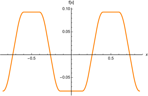
  Figure 1: Plot of $f[x]$ for $\{\Delta_{F_{1}},\Delta_{F_{2}},\Delta_{B}\}\,=\,\{0.04\,,0.9\,,0.27\}$

• $\mathbf{\Delta_{B}\leq\Delta_{F_{1}}+\Delta_{F_{2}}}$: In this case the fundamental domain is $|x|<1-\Delta_{F_{1}}-\Delta_{F_{2}}+\Delta_{B}$ and $f[x]$ reads:

  $$\begin{split}&f[x]=\\ &\left\{\begin{array}[]{lr}12(\Delta_{B}^{2}+(\Delta_{F_{1}}-\Delta_{F_{2}})^{2}-2\Delta_{B}\Delta_{F_{2}}+\Delta_{B}\Delta_{F_{1}}(8\Delta_{F_{2}}-2)+x^{2})&0<x<x_{1}\\ 6((x+\Delta_{F_{1}}+\Delta_{F_{2}}-\Delta_{B})^{2}-8(1-2\Delta_{B})\Delta_{F_{1}}\Delta_{F_{2}})&x_{1}<x<x_{2}\\ 24\Delta_{F_{1}}(x-\Delta_{F_{2}}+\Delta_{B}(4\Delta_{F_{2}}-1))&x_{2}<x<x_{3}\\ 6(16\Delta_{B}\Delta_{F_{1}}\Delta_{F_{2}}-(x-\Delta_{F_{1}}-\Delta_{F_{2}}-\Delta_{B})^{2})&x_{3}<x<x_{4}\\ 96\Delta_{B}\Delta_{F_{1}}\Delta_{F_{2}}&x>x_{4}\\ \end{array}\right.\end{split}$$ (36)

  where $x_{1}=\Delta_{F_{1}}+\Delta_{F_{2}}-\Delta_{B}$, $x_{2}=\Delta_{B}+\Delta_{F_{1}}-\Delta_{F_{2}}$, $x_{3}=\Delta_{B}-\Delta_{F_{1}}+\Delta_{F_{2}}$, and $x_{4}=\Delta_{B}+\Delta_{F_{1}}+\Delta_{F_{2}}$. This time, we can observe that $f[x]$ is manifestly non-constant in a neighborhood of $x=0$, where a unique minimum is located (see figure 2).

  

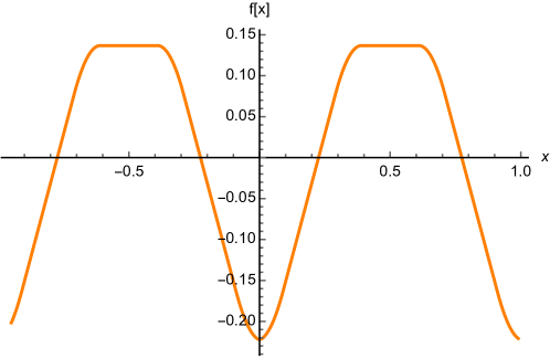
  Figure 2: Plot of $f[x]$ for $\{\Delta{F_{1}},\Delta_{F_{2}},\Delta_{B}\}\,=\,\{0.05\,,0.15\,,0.19\}$

  Reminding that $V_{2}$ is actually, $-f[x]-f[y]$, we discover that this extremal point $a_{+}=a_{-}=0$, i.e. vanishing holonomies, dominates the Cardy-like limit in the regime:

  $$\text{Re}\left(\frac{i}{\omega_{1}\omega_{2}}\right)>0\,.$$ (37)

We showed that not all the chambers lead to honest isolated extrema and a similar analysis must be always performed. A numerical analysis for higher ranks still validates the work-hypothesis of vanishing holonomies and from now on we will consider arbitrary rank $N$ following this assumption.

In order to exploit the geometric insight, from now on we prefer to take a suitable basis of field charges that are directly suggested by the toric diagram, as discussed in section 2; in this basis flavour and baryonic symmetries get mixed and can be considered on equal footing. We will label the three $U(1)$ global symmetries simply as $U(1)_{1,2,3}$ and the associated fugacities as $\Delta_{1,2,3}$; $R$-symmetry will be denoted by $U(1)_{R}$ instead. Following the discussion in section 2 we can parameterize the global charges from the geometry using perfect matchings.

In this case there are four perfect matchings associated to the four external points of the toric diagram. They are listed in (38), where it is possible to observe that in this case each PM corresponds to a bifundamental chiral field. The charges of these fields can be parameterized in terms of the PMs as

$$\begin{array}[]{c|c|c|c}A_{1}&B_{1}&A_{2}&\quad B_{2}\\ \hline\cr{\quad\bf a_{1}}&{\quad\bf a_{2}}&{\quad\bf a_{3}}&{\quad\bf a_{4}}\end{array}$$ (39)

The charges of the fields with respect to the symmetries suggested by the geometric data can be taken then as follows

$$U(1)_{1}$$

(40)

We want to stress that, as in the $\mathcal{N}=4$ case discussed in section 2, the $R$-symmetry that we consider here accidentally coincides with the exact $R$-symmetry at the conformal fixed point. However this will not be the case in the models that we are going to discuss in the next section. Observe that the new conjugated fugacities $\Delta_{i}$ can thought as linear combination of the flavour and baryonic ones:

$$\Delta_{1}\,=\,\Delta_{B}+\Delta_{F_{1}}+\Delta_{F_{2}}\,,\quad\Delta_{2}\,=\,-\Delta_{B}+\Delta_{F_{1}}-\Delta_{F_{2}}\,,\quad\Delta_{3}\,=\,\Delta_{B}-\Delta_{F_{1}}-\Delta_{F_{2}}\,.$$ (41)

$V_{2}$ for arbitrary rank can be now expressed as:

$$\begin{split}V_{2}\,=\,-\sum_{m,n=1}^{N}&\left(\kappa\left[a^{(1)}_{m}-a^{(2)}_{n}+\Delta_{1}\right]+\kappa\left[a^{(2)}_{m}-a^{(1)}_{n}+\Delta_{2}\right]+\right.\\ &\left.\,\,\,\,\kappa\left[a^{(1)}_{m}-a^{(2)}_{n}+\Delta_{3}\right]+\kappa\left[a^{(2)}_{m}-a^{(1)}_{n}-\Delta_{1}-\Delta_{2}-\Delta_{3}\right]\right)\,.\end{split}$$ (42)

In this basis we fix the fugacities such that $0\leq\Delta_{1,2,3}<1/2$ and $0\leq\Delta_{1}+\Delta_{2}+\Delta_{3}\leq 1/2$. In this chamber, $f[x]$ enjoys a local maximum for vanishing holonomies and thus $V_{2}$ exhibits a minimum. The extremum dominates the Cardy-like limit if

$$\text{Re}\left(\frac{i}{\omega_{1}\omega_{2}}\right)<0\,.$$ (43)

In the fixed regime, we can evaluate the dominant saddle contribution:

$$\begin{split}V\,=&\,\frac{i\,\pi}{2\omega_{1}\omega_{2}}\left(\frac{V_{2}}{3}+(\omega_{1}+\omega_{2})V_{1}\right)\bigg{|}_{a^{(I)}_{m}=0}\,=\,\\ =&\frac{\pi i\,N^{2}}{2\omega_{1}\omega_{2}}\left\{(\omega_{1}+\omega_{2})\left(\Delta_{3}(\Delta_{3}-1)+\Delta_{1}(\Delta_{2}+\Delta_{3}-1)+\Delta_{1}^{2}+\Delta_{2}^{2}+\Delta_{2}(\Delta_{3}-1)\right)+\right.\\ &\left.-\left(\Delta_{2}\Delta_{3}(\Delta_{2}+\Delta_{3}-1)+\Delta_{1}^{2}(\Delta_{2}+\Delta_{3}+\Delta_{1}(\Delta_{2}+\Delta_{3}-1)(\Delta_{2}+\Delta_{3}))\right)\right\}\,.\end{split}$$ (44)

This equation get further simplified performing a suitable shift of the fugacities

$$\Delta_{1,2,3}\,\rightarrow\,\Delta_{1,2,3}-\frac{\omega_{1}+\omega_{2}}{4}$$ (45)

and taking the leading order in the Cardy-like limit $|\omega_{1}|,|\omega_{2}|\rightarrow 0\,\,$; let us stress that the shift (45) is actually dictated by the geometry: as we will test for other toric models in the next sections, the fugacities get always shifted by $-\frac{\omega_{1}+\omega_{2}}{d}$ where $d$ is the number of external points in the toric diagram. After the shift, the entropy function can be expressed as

$$S_{E}\,=\,-\frac{i\pi N^{2}}{\omega_{1}\omega_{2}}(\Delta_{1}\Delta_{2}\Delta_{3}+\Delta_{1}\Delta_{2}\Delta_{4}+\Delta_{1}\Delta_{3}\Delta_{4}+\Delta_{2}\Delta_{3}\Delta_{4})\,,$$ (46)

where we have defined:

$$\Delta_{4}\,\equiv\,\omega_{1}+\omega_{2}+1-\Delta_{1}-\Delta_{2}-\Delta_{3}\,.$$ (47)

The entropy function (46) enjoys the expected scaling behaviour $S_{E}\,\propto N^{2}$; moreover, it is in perfect agreement with our general proposal

$$S_{E}\,=\,-\frac{i\pi N^{2}}{6\,\omega_{1}\omega_{2}}C_{IJK}\Delta_{I}\Delta_{J}\Delta_{K}\,,$$ (48)

where $I,J,K$ run from $1$ to $4$ and $C_{IJK}$ is defined as in (3).

4 Other examples

In this section we test our proposal (20) in various cases of growing complexity. In each case we assign the charges using the prescription discussed in section 2 and we assume that the Cardy-like limit is dominated by a unique minimum where all the holonomies vanish. We have tested the last conjecture in the rank-1 cases of $\text{dP}_{1}$,$\text{dP}_{2},\text{(P)dP}_{4}$ and $\mathbb{F}_{0}$, finding evidence of its validity. In each case the minimum is found in a chamber where fugacities $\Delta_{i}$ of the $d-1$ U(1) global symmetries are taken such that:

$$0\leq\Delta_{i}\leq\frac{1}{2}\,\,\,\forall i\,,\quad 0\leq\sum_{i=1}^{d-1}\,\Delta_{i}\,\leq 1\,.$$ (49)

Since in this range $V_{2}$ enjoys a minimum, we restrict to the regime (43).

As a general remark let us stress that some of the theories that we are going to discuss admit more Seiberg dual realizations, denoted as phases. We specify for each model the Seiberg phase that we focus on. Finally, observe that we are not necessarily fixing the $R$-charges of the fields at the conformal fixed point, but we refer to a trial $R$-current, using the uniform prescription for all the models under investigation, as explained in section 2.

4.1 SPP

The suspended pinch point (SPP) gauge theory corresponds to the near horizon limit of a stack of $N$ D3 branes probing the tip of the conical singularity, $x^{2}y=wz$. This is the simplest example of a larger class of models, defined by the equation $x^{a}y^{b}=wz$, denoted as $L^{aba}$ models. In the SPP case the toric Sasaki-Einstein base in described by the following vectors:

$$V_{1}=(1,1,1),\quad V_{2}=(1,0,1),\quad V_{3}=(0,0,1),\quad V_{4}=(2,0,1),\quad V_{5}=(1,0,1)\,.$$ (50)

The vector $V_{5}$ represents a point on the perimeter of the toric diagram and it turns out that two different perfect matchings can be associated to it and, consequently, we can get two different possible charge sets. Following the prescription of Butti:2005vn we can associate a non vanishing set of charges to just one of them.

The theory living on a stack of $N$ D3-branes at the SPP conical singularity is described by the following quiver:

with superpotential

$$W=\text{Tr}[X_{21}X_{12}X_{23}X_{32}-X_{32}X_{23}X_{31}X_{13}+X_{13}X_{31}\phi-X_{12}X_{21}\phi].$$ (52)

Each $X_{ij}$ transforms in the $\mathbf{N}$ representation of the $i$ node and in the $\overline{\mathbf{N}}$ of the $j$-th node; the field transforming in the adjoint of the first node is named, instead, $\phi$. The charges of the fields can be parameterized in terms of the PMs using the assignation

$$\begin{array}[]{c|c|c|c|c|c|c}\phi&X_{12}&X_{21}&X_{23}&X_{32}&X_{31}&X_{13}\\ \hline\cr\mathbf{\quad a_{1}+a_{2}\quad}&\mathbf{\quad a_{4}\quad}&\mathbf{\quad a_{3}+a_{5}\quad}&\mathbf{\quad a_{2}\quad}&\mathbf{\quad a_{1}\quad}&\mathbf{\quad a_{4}+a_{5}\quad}&\mathbf{\quad a_{3}\quad}\end{array}$$ (53)

It follows that the charge assignment for $U(1)_{R}$ and the extra four $U(1)_{i}$ global can be taken as follows:

$$U(1)_{1}$$

1 1 0 0 4/5

0 0 0 1 2/5

-1 -1 0 -1 4/5

0 1 0 0 2/5

1 0 0 0 2/5

-1 -1 -1 0 4/5

0 0 1 0 2/5

(54)

Observe that as usual we took a combination of $U(1)$ natural for toric geometry and we have not done any distinction between flavour and baryonic symmetries. We denote $\Delta_{i}$ the fugacity associated to $U(1)_{i}$. With this assignment, $V_{2}$ admits a minimum for vanishing holonomies in a chamber where $0\leq\Delta_{i}\leq 1/2$ for each $U(1)_{i}$ and $0<\Delta_{1}+\Delta_{2}+\Delta_{3}+\Delta_{4}<1$; we can evaluate

$$V=\frac{i\pi}{2\omega_{1}\omega_{2}}\left(V_{1}(\omega_{1}+\omega_{2})+\frac{V_{2}}{3}\right)$$ (55)

and, after performing a shift of the charges by a factor $-\tfrac{\omega_{1}+\omega_{2}}{5}$ and taking the leading order in $|\omega_{1}|,|\omega_{2}|\rightarrow 0$, we get:

$$\begin{split}V_{\text{leading}}\,=\,\frac{i\pi N^{2}}{\omega_{1}\omega_{2}}&\left(\Delta_{1}((\Delta_{2}+\Delta_{3})(\Delta_{2}+\Delta_{3}\!-\!\omega_{1}\!-\!\omega_{2}\!-\!1)+\Delta_{4}^{2}\!-\!\Delta_{4}(1\!+\!\omega_{1}\!+\!\omega_{2}\!-\!2\Delta_{2}))\right.\\ &\left.\,\,\,\,+\Delta_{2}(\Delta_{3}^{2}-\Delta_{3}(1+\omega_{1}+\omega-\Delta_{2})+\Delta_{4}(\Delta_{2}+\Delta_{4}-1-\omega_{1}-\omega_{2}))+\right.\\ &\,\,\,\,\left.+\Delta_{1}^{2}(\Delta_{2}+\Delta_{3}+\Delta_{4})\right).\end{split}$$ (56)

If we now define a new constrained fugacity:

$$\quad\Delta_{5}\,=\,1+\omega_{1}+\omega-\Delta_{1}-\Delta_{2}-\Delta_{3}-\Delta_{4}$$ (57)

we obtain the following expression for the entropy:

$$\begin{split}S_{E}=-\frac{i\pi N^{2}}{\omega_{1}\omega_{2}}&\left(\Delta_{1}\Delta_{2}\Delta_{3}+\Delta_{1}\Delta_{2}\Delta_{4}+2\Delta_{1}\Delta_{3}\Delta_{4}+2\Delta_{2}\Delta_{3}\Delta_{4}+\right.\\ &\,\,\,\,\left.+\Delta_{1}\Delta_{2}\Delta_{5}+\Delta_{1}\Delta_{3}\Delta_{5}+\Delta_{2}\Delta_{3}\Delta_{5}+\Delta_{1}\Delta_{4}\Delta_{5}+\Delta_{2}\Delta_{4}\Delta_{5}\right)\,.\end{split}$$ (58)

This result is in agreement with our expectation from toric geometry, encoded in formula (20).

Finally, as discussed at the beginning of this section, the SPP singularity can be thought as a particular case of a larger class of toric models, denoted as $L^{aba}$, for $a=1\,,b=2$. The toric diagram of an $L^{aba}$ singularity is depicted in (59).

$$\scalebox{0.8}{ \leavevmode\hbox to123.98pt{\vbox to66.68pt{\text{[drawing]}}}}\quad\Rightarrow\quad\scalebox{0.8}{ \leavevmode\hbox to180.88pt{\vbox to98.25pt{\text{[drawing]}}}} \bullet \bullet \bullet \bullet \bullet \bullet \bullet \bullet \bullet \bullet \bullet a-1 b-1 \bullet \bullet \bullet \bullet \bullet \bullet \bullet \bullet \bullet \bullet \bullet \bullet \bullet a-1 b-1 \bullet \bullet$$ (59)

In this case there are $a+b$ gauge groups, and two flavor symmetries and $a+b-1$ non anomalous baryonic symmetries. This huge amount of baryonic symmetries reflects in the toric diagram onto the large number of external point lying on the perimeter. Each of these points contribute with triangle areas to reproduce the correct entropy function, following the general prescription (20). Observe that for $a=0$ the models become $\mathcal{N}=2$ necklace quivers, corresponding to $\mathbb{Z}_{b}$ orbifolds of $\mathcal{N}=4$ SYM. The entropy for these models has been studied in Honda:2019cio , by turning off the baryonic fugacities. Here in section 6 we will study the most general situation.

4.2 $\mathbb{F}_{0}$

The complex cone over the first Hirzebruch surface $\mathbb{F}_{0}$ is a $\mathbb{Z}_{2}$ orbifold of the conifold; the toric diagram is parametrized by the four vectors

$$V_{1}=(0,0,1),\quad V_{2}=(1,0,1),\quad V_{3}=(0,2,1),\quad V_{4}=(-1,2,1).$$ (60)

The corresponding theory in its phase $I$ is described by the following quiver and superpotential:

$$\scalebox{1.2}{ \leavevmode\hbox to101.08pt{\vbox to93.85pt{\text{[drawing]}}}}\quad\quad W=\epsilon_{\alpha\beta}\epsilon_{\gamma\delta}\text{Tr}[X^{(\alpha)}_{12}X^{(\beta)}_{34}X^{(\gamma)}_{23}X^{(\delta)}_{41}]. \bullet \bullet \bullet \bullet X^{(\alpha)}_{34} X^{(\alpha)}_{41} X^{(\alpha)}_{23} X^{(\alpha)}_{12} \bullet \bullet \bullet \bullet X^{(\alpha)}_{34} X^{(\alpha)}_{41} X^{(\alpha)}_{23} X^{(\alpha)}_{12}$$ (61)

One can assign charges to the fields in the theory directly from the geometry. The charges of the fields can be parameterized in terms of the PMs using the assignation

$$\begin{array}[]{c|c|c|c}X_{12}&X_{34}&X_{23}&X_{41}\\ \hline\cr{\bf a_{1}}&{\bf a_{2}}&{\bf a_{3}}&{\bf a_{4}}\end{array}$$ (62)

The model has three global $U(1)$ symmetries in addition to one $U(1)_{R}$ and in this case one gets the following global charges

$$\begin{array}[]{c|c|cccc}&\text{multiplicity}&\,U(1)_{1}&U(1)_{2}&U(1)_{3}&U(1)_{R}\\ \hline\cr X_{12}&2&1&0&0&1/2\\ X_{23}&2&0&1&0&1/2\\ X_{34}&2&0&0&1&1/2\\ X_{41}&2&-1&-1&-1&1/2\\ \end{array}$$ (63)

We now compute the Cardy-like limit of the superconformal index for this theory; if we denote the fugacities for the symmetries $U(1)_{1,2,3}$ as $\Delta_{1,2,3}$ respectively, the expression that we find after shifting each fugacity by $-\tfrac{\omega_{1}+\omega_{2}}{4}$ is

$$\begin{split}V_{\text{leading}}=-\frac{2\pi iN^{2}}{\omega_{1}\omega_{2}}\bigl{(}&\Delta_{2}(1+\omega_{1}+\omega_{2}-\Delta_{2}-\Delta_{3})\Delta_{3}-\Delta_{1}^{2}(\Delta_{2}+\Delta_{3})\\ &\bigl{.}-\Delta_{1}(\Delta_{2}+\Delta_{3})(1+\omega_{1}+\omega_{2}-\Delta_{2}-\Delta_{3})\bigr{)}\end{split}$$ (64)

The entropy function in this case can be written as:

$$S_{E}(\Delta,\omega)=-\frac{2\pi iN^{2}}{\omega_{1}\omega_{2}}(\Delta_{1}\Delta_{2}\Delta_{3}+\Delta_{1}\Delta_{2}\Delta_{4}+\Delta_{1}\Delta_{3}\Delta_{4}+\Delta_{2}\Delta_{3}\Delta_{4}),$$ (65)

and it exactly reproduces (64) by using the constraint

$$\Delta_{4}=1+\omega_{1}+\omega_{2}-\Delta_{1}-\Delta_{2}-\Delta_{3},$$ (66)

Observe that the entropy function just obtained is twice the one for the conifold, as one should expect from the fact that we are dealing with a $\mathbb{Z}_{2}$ orbifold of the latter .

4.3 dP₁

Let us consider the theory arising from a stack of $N$ D3 branes at the tip of the complex Calabi-Yau cone whose base is the first del Pezzo surface. The toric diagram is generated by

$$V_{1}=(1,0,1),\quad V_{2}=(0,1,1),\quad V_{3}=(-1,0,1),\quad V_{4}=(-1,-1,1).$$ (67)

The corresponding quiver is as follows

and the superpotential for this theory reads

$$W=\epsilon_{\alpha\beta}\text{Tr}[X^{(\alpha)}_{34}X^{(\beta)}_{41}X_{13}-X^{(\alpha)}_{34}X^{(\beta)}_{23}X_{42}+X_{12}X^{(3)}_{34}X^{(\alpha)}_{41}X^{(\beta)}_{23}].$$ (69)

The charges of the fields can be parameterized in terms of the PMs using the assignation

$$\begin{array}[]{c|c|c|c|c|c}X_{34}^{(3)},X_{13},X_{42}&X_{23}^{(1)},X_{41}^{(1)}&X_{12}&X_{23}^{(2)},X_{41}^{(2)}&X_{34}^{(1)}&X_{34}^{(2)}\\ \hline\cr{\bf a_{1}}&{\bf a_{2}}&{\bf a_{3}}&{\bf a_{4}}&{\bf a_{2}+a_{3}}&{\bf a_{3}+a_{4}}\end{array}$$ (70)

The charges for $U(1)_{R}$ and the three global $U(1)$ symmetries of the model coming from the perfect matching are the following

$$\begin{array}[]{c|cccc}&U(1)_{1}&U(1)_{2}&U(1)_{3}&U(1)_{R}\\ \hline\cr X_{12}&0&0&1&1/2\\ X_{23}^{(1)}&0&1&0&1/2\\ X_{23}^{(2)}&-1&-1&-1&1/2\\ \hline\cr X_{34}^{(1)}&0&1&1&1\\ X_{34}^{(2)}&-1&-1&0&1\\ X_{34}^{(3)}&1&0&0&1/2\\ \hline\cr X_{41}^{(1)}&0&1&0&1/2\\ X_{41}^{(2)}&-1&-1&-1&1/2\\ \hline\cr X_{13}&1&0&0&1/2\\ X_{42}&1&0&0&1/2\\ \end{array}$$ (71)

The expression for the entropy function in this case gives:

$$S_{E}(\Delta,\omega)=-\frac{i\pi N^{2}}{\omega_{1}\omega_{2}}(2\Delta_{1}\Delta_{2}\Delta_{3}+2\Delta_{1}\Delta_{2}\Delta_{4}+2\Delta_{1}\Delta_{3}\Delta_{4}+\Delta_{2}\Delta_{3}\Delta_{4}).$$ (72)

Again, the same result can be obtained by taking the Cardy-like limit of the superconformal index. The leading order of the function

$$V=\frac{i\pi N^{2}}{2\omega_{1}\omega_{1}}\left(V_{1}(\omega_{1}+\omega_{2})+\frac{V_{2}}{3}\right),$$ (73)

taken after shifting the charges by a factor $-\tfrac{\omega_{1}+\omega_{2}}{4}$, is given by

$$\begin{split}V_{\text{leading}}=\frac{i\pi N^{2}}{\omega_{1}\omega_{2}}&\bigl{(}3\Delta_{1}\Delta_{2}(\Delta_{1}+\Delta_{2}-\omega_{1}-\omega_{2}-1)-2\Delta_{1}\Delta_{3}(1+\omega_{1}+\omega_{2}-\Delta_{1})\bigr{.}\\ &-(1+\omega_{1}+\omega_{2}-4\Delta_{1})\Delta_{2}\Delta_{3}+\Delta_{2}^{2}\Delta_{3}+(2\Delta_{1}+\Delta_{2})\Delta_{3}^{2}\bigr{)}.\end{split}$$

If we now take the expression of the entropy function (72) and impose the constraint on the fugacities

$$\Delta_{4}=1+\omega_{1}+\omega_{2}-\Delta_{1}-\Delta_{2}-\Delta_{3},$$ (74)

we obtain the expression (4.3) for the entropy function.

4.4 dP₂

The toric diagram for the complex cone over the dP₂ surface is generated by the following vectors

$$V_{1}=(1,1,1),\quad V_{2}=(0,1,1),\quad V_{3}=(-1,0,1),\quad V_{4}=(-1,-1,1),\quad V_{5}=(0,-1,1).$$ (75)

The charges of the fields can be parameterized in terms of the PMs using the assignation

$$\begin{array}[]{c|c|c|c|c|c|c|c|c|c|c}X_{13}&X_{24}&X_{51}^{(1)}&X_{23}&X_{41}&X_{51}^{(2)}&X_{12}^{(2)}&X_{45}&X_{12}^{(1)}&X_{35}&X_{34}\\ \hline\cr{\bf a_{4}+a_{5}}&{\bf a_{5}}&{\bf a_{5}}&{\bf a_{2}}&{\bf a_{1}+a_{2}}&{\bf a_{2}+a_{3}}&{\bf a_{3}+a_{4}}&{\bf a_{4}}&{\bf a_{1}}&{\bf a_{1}}&{\bf a_{3}}\end{array}$$ (76)

The theory arising from a stack of $N$ D3 branes put at the tip of this toric Calabi-Yau cone admits two phases. The phase $I$ can be described by a quiver with five nodes

and superpotential

$$\begin{split}W=\text{Tr}\bigl{[}&X_{13}X_{34}X_{41}-X_{12}^{(2)}X_{24}X_{41}+X_{12}^{(1)}X_{24}X_{45}X_{51}^{(2)}-X_{13}X_{35}X_{51}^{(2)}\bigr{.}\\ &\bigl{.}+X_{12}^{(2)}X_{23}X_{35}X_{51}^{(1)}-X_{12}^{(1)}X_{23}X_{34}X_{45}X_{51}^{(1)}\bigr{]}.\end{split}$$ (78)

Here $X_{ij}$ denotes a bifundamental field connecting the $i$-th and $j$-th nodes. The charges assigned to the various fields in the quiver directly from the perfect matchings are

$$\begin{array}[]{c|ccccc}&U(1)_{1}&U(1)_{2}&U(1)_{3}&U(1)_{4}&U(1)_{R}\\ \hline\cr X_{13}&-1&-1&-1&0&4/5\\ X_{24}&-1&-1&-1&-1&2/5\\ X_{51}^{(1)}&-1&-1&-1&-1&2/5\\ X_{23}&0&1&0&0&2/5\\ X_{41}&1&1&0&0&4/5\\ X_{51}^{(2)}&0&1&1&0&4/5\\ X_{12}^{(2)}&0&0&1&1&4/5\\ X_{45}&0&0&0&1&2/5\\ X_{12}^{(1)}&1&0&0&0&2/5\\ X_{35}&1&0&0&0&2/5\\ X_{34}&0&0&1&0&2/5\\ \end{array}$$ (79)

The entropy function obtained from toric geometry is:

$$\begin{split}S_{E}(\Delta,\omega)=-\frac{i\pi N^{2}}{\omega_{1}\omega_{2}}\bigl{(}&\Delta_{1}\Delta_{2}\Delta_{3}+2\Delta_{1}\Delta_{2}\Delta_{4}+2\Delta_{1}\Delta_{3}\Delta_{4}+\Delta_{2}\Delta_{3}\Delta_{4}\bigr{.}\\ &\bigl{.}+2\Delta_{1}\Delta_{2}\Delta_{5}+3\Delta_{1}\Delta_{3}\Delta_{5}+3\Delta_{1}\Delta_{3}\Delta_{5}+2\Delta_{2}\Delta_{3}\Delta_{5}\bigr{.}\\ &+\bigl{.}2\Delta_{1}\Delta_{4}\Delta_{5}+2\Delta_{2}\Delta_{4}\Delta_{5}+\Delta_{3}\Delta_{4}\Delta_{5}\bigr{)}\end{split}$$ (80)

The leading order of the Cardy-like limit of the superconformal index gives, after shifting the charges by a factor $-\tfrac{\omega_{1}+\omega_{2}}{5}$

$$\begin{split}V_{\text{leading}}=\frac{i\pi}{\omega_{1}\omega_{2}}&\Bigl{[}(2\Delta_{2}^{2}(\Delta_{3}+\Delta_{4})+(\Delta_{3}\Delta_{4}+2\Delta_{2}(\Delta_{3}+\Delta_{4}))(\Delta_{3}+\Delta_{4}\!-\!1\!-\!\omega_{1}\!-\!\omega_{2})\Bigr{.}+\\ \Bigl{.}&+\Delta_{1}^{2}(2\Delta_{2}+3\Delta_{3}+2\Delta_{4})+2\Delta_{1}\Delta_{2}^{2}-3\Delta_{1}\Delta_{3}(1+\omega_{1}+\omega_{2}-\Delta_{3})+\Bigr{.}\\ &\Bigl{.}-2\Delta_{1}\Delta_{2}(1+\omega_{1}+\omega_{1}-3\Delta_{3}-2\Delta_{4})-2\Delta_{1}\Delta_{4}(1+\omega_{1}+\omega_{2}-2\Delta_{3})\Bigr{.}\\ &\Bigl{.}+2\Delta_{1}\Delta_{4}^{2}\Bigr{]}.\end{split}$$ (81)

This is the same expression that one gets by taking (80) and using the constraint on the fugacities

$$\Delta_{5}=-\Delta_{1}-\Delta_{2}-\Delta_{3}-\Delta_{4}+\omega_{1}+\omega_{2}+1.$$ (82)

4.5 dP₃

The toric diagram for the Calabi-Yau cone over the dP₃ surface is generated by the following vectors

$$\begin{split}&V_{1}=(1,1,1),\quad\quad\;\;V_{2}=(0,1,1),\quad\;\;\;V_{3}=(-1,0,1),\\ &V_{4}=(-1,-1,1),\quad V_{5}=(0,-1,1),\quad V_{6}=(1,0,1).\end{split}$$ (83)

The charges of the fields can be parameterized in terms of the PMs using the assignation

$$\begin{array}[]{c|c|c|c|c|c|c|c|c|c|c|c}X_{12}&X_{13}&X_{23}&X_{24}&X_{34}&X_{35}&X_{45}&X_{46}&X_{56}&X_{51}&X_{61}&X_{62}\\ \hline\cr{\bf a_{6}}&{\bf a_{2}+a_{3}}&{\bf a_{5}}&{\bf a_{1}+a_{2}}&{\bf a_{4}}&{\bf a_{1}+a_{6}}&{\bf a_{3}}&{\bf a_{5}+a_{6}}&{\bf a_{2}}&{\bf a_{4}+a_{5}}&{\bf a_{1}}&{\bf a_{3}+a_{4}}\end{array}$$ (84)

The theory associated to this cone admits three phases; in its phase $I$, it can be described by the following quiver:

with superpotential

$$\begin{split}W=\text{Tr}\bigl{[}&X_{12}X_{24}X_{45}X_{51}-X_{24}X_{46}X_{62}+X_{23}X_{35}X_{56}X_{62}\bigr{.}\\ &\bigl{.}-X_{35}X_{51}X_{13}+X_{34}X_{46}X_{61}X_{13}-X_{12}X_{23}X_{34}X_{45}X_{56}X_{61}\bigr{]},\end{split}$$ (86)

where $X_{ij}$ denotes a bifundamental field connecting the $i$-th and $j$-th nodes. The charges assigned from the toric diagram to the various fields in the theory are

$$\begin{array}[]{c|cccccc}&U(1)_{1}&U(1)_{2}&U(1)_{3}&U(1)_{4}&U(1)_{5}&U(1)_{R}\\ \hline\cr X_{12}&-1&-1&-1&-1&-1&1/3\\ X_{13}&0&1&1&0&0&2/3\\ X_{23}&0&0&0&0&1&1/3\\ X_{24}&1&1&0&0&0&2/3\\ X_{34}&0&0&0&1&0&1/3\\ X_{35}&0&-1&-1&-1&-1&2/3\\ X_{45}&0&0&1&0&0&1/3\\ X_{46}&-1&-1&-1&-1&0&2/3\\ X_{56}&0&1&0&0&0&1/3\\ X_{51}&0&0&0&1&1&2/3\\ X_{61}&1&0&0&0&0&1/3\\ X_{62}&0&0&1&1&0&2/3\\ \end{array}$$ (87)

The entropy function for this theory is

$$\begin{split}S_{E}(\Delta,\omega)=-\frac{i\pi N^{2}}{\omega_{1}\omega_{2}}\bigl{(}&\Delta_{1}\Delta_{2}\Delta_{3}+2\Delta_{1}\Delta_{2}\Delta_{4}+2\Delta_{1}\Delta_{3}\Delta_{4}+\Delta_{2}\Delta_{3}\Delta_{4}+2\Delta_{1}\Delta_{2}\Delta_{5}\bigr{.}\\ &\bigl{.}+3\Delta_{1}\Delta_{3}\Delta_{5}+2\Delta_{2}\Delta_{3}\Delta_{5}+2\Delta_{1}\Delta_{4}\Delta_{5}+2\Delta_{2}\Delta_{4}\Delta_{5}+\Delta_{3}\Delta_{4}\Delta_{5}\bigr{.}\\ &\bigl{.}+\Delta_{1}\Delta_{2}\Delta_{6}+2\Delta_{1}\Delta_{3}\Delta_{6}+2\Delta_{2}\Delta_{3}\Delta_{6}+2\Delta_{1}\Delta_{4}\Delta_{6}+3\Delta_{2}\Delta_{4}\Delta_{6}\bigr{.}\\ &\bigl{.}+2\Delta_{3}\Delta_{4}\Delta_{6}+\Delta_{1}\Delta_{5}\Delta_{6}+2\Delta_{2}\Delta_{5}\Delta_{6}+2\Delta_{3}\Delta_{5}\Delta_{6}+\Delta_{4}\Delta_{5}\Delta_{6}\bigr{)}.\end{split}$$ (88)

In fact, evaluating $V$ at the leading order in $|\omega_{1}|,|\omega_{2}|\rightarrow 0$ we get

$$\begin{split}V_{\text{leading}}=-\frac{i\pi N^{2}}{\omega_{1}\omega_{2}}\bigl{(}&2\Delta_{3}\Delta_{4}(1\!+\!\omega_{1}\!+\!\omega_{2}\!-\!\Delta_{3}\!-\!\Delta_{4})\!-\!2\Delta_{3}^{2}\Delta_{5}\!+\!2\Delta_{3}\Delta_{5}(1\!+\!\omega_{1}\!+\!\omega_{2}\!-\!2\Delta_{4})\bigr{.}\\ &\bigl{.}+\Delta_{4}\Delta_{5}(1\!+\!\omega_{1}\!+\!\omega_{2}\!-\!\Delta_{4})\!+\!\Delta_{5}^{2}(2\Delta_{3}\!+\!\Delta_{4})\!\!-\!\!\Delta_{1}^{2}(\Delta_{2}\!+\!2\Delta_{3}\!+\!2\Delta_{4}\!+\!\Delta_{5})\bigr{.}\\ &\bigl{.}-\Delta_{2}^{2}(2\Delta_{3}+3\Delta_{4}+2\Delta_{5})-2\Delta_{2}\Delta_{3}^{2}+3\Delta_{2}\Delta_{4}(1+\omega_{1}+\omega_{2}-\Delta_{4})\bigr{.}\\ &\bigl{.}+2\Delta_{2}\Delta_{3}(1+\omega_{1}+\omega_{2}-3\Delta_{4}-2\Delta_{5})+2\Delta_{2}\Delta_{5}(1+\omega_{1}+\omega_{2}-2\Delta_{4})\bigr{.}\\ &\bigl{.}-2\Delta_{2}\Delta_{5}^{2}-\Delta_{1}\Delta_{2}^{2}-2\Delta_{1}(\Delta_{3}+\Delta_{4})(\Delta_{3}+\Delta_{4}-1-\omega_{1}-\omega_{2})\bigr{.}\\ &\bigl{.}+\Delta_{1}\Delta_{2}(1+\omega_{1}+\omega_{2}-4\Delta_{3}-4\Delta_{4}-2\Delta_{5})-\Delta_{1}\Delta_{5}^{2}\bigr{.}\\ &\bigl{.}+\Delta_{1}\Delta_{5}(1+\omega_{1}+\omega_{2}-2\Delta_{3}-2\Delta_{4})\bigr{)},\end{split}$$ (89)

where we also shifted the fugacities by $-\frac{\omega_{1}+\omega_{2}}{6}$, consistently with the general prescription. Again, by imposing the constraint

$$\Delta_{6}=-\Delta_{1}-\Delta_{2}-\Delta_{3}-\Delta_{4}-\Delta_{5}+\omega_{1}+\omega_{2}+1,$$ (90)

on (89) we obtain (88).

4.6 $\text{(P)dP}_{4}$

The fourth del Pezzo surface is defined as the blow-up of $\mathbb{P}^{2}$ at four generic points. The (complex) cone over it possesses a Calabi-Yau structure and the theory living on $N$ D3-branes probing the conical singularity is known; however the superpotential of the dual gauge theory is such that no non-anomalous flavour symmetries except $U(1)_{R}$ are admitted, so that the model is non-toric. Blowing-up $\mathbb{P}^{2}$ at non-generic points, however, it is possible to build models where more symmetries are preserved.

One choice can be the toric model whose diagram is generated by the following vectors:

$$\begin{split}&V_{1}\,=\,(0,0,1)\,,V_{2}\,=\,(1,0,1)\,,V_{3}\,=\,(2,0,1)\,,V_{4}\,=\,(2,1,1)\,,\\ &V_{5}\,=\,(1,2,1)\,,V_{6}\,=\,(0,2,1)\,,V_{7}\,=\,(0,1,1)\,,\end{split}$$ (91)

and that we will denote as pseudo $\text{dP}_{4}$ or $\text{(P)dP}_{4}$. The dual gauge theory can be described by the following quiver:

with superpotential:

$$\begin{split}W\,=\,\text{Tr}&\left[X_{61}X_{17}X_{74}X_{46}+X_{21}X_{13}X_{35}X_{52}+X_{27}X_{73}X_{36}X_{62}+X_{14}X_{45}X_{51}\right.+\\ &\,\,\,\,-X_{51}X_{17}X_{73}X_{35}-X_{21}X_{14}X_{46}X_{62}-X_{27}X_{74}X_{45}X_{52}-X_{13}X_{36}X_{61}\left.\right]\,,\end{split}$$ (93)

where each $X_{ij}$ must be understood as a field transforming in the bifundamental representation with respect to the $i$-th and $j$-th nodes. The charges of the fields can be parameterized in terms of the PMs using the assignation

$$\begin{split}\begin{array}[]{c|c|c|c|c|c|c|c}X_{17}&X_{21}&X_{27}&X_{73}&X_{14}&X_{74}&X_{13}&X_{62}\\ \hline\cr{\bf a_{1}+a_{6}+a_{7}}&{\bf a_{7}}&{\bf a_{3}+a_{4}}&{\bf a_{2}}&{\bf a_{1}+a_{2}+a_{3}}&{\bf a_{5}}&{\bf a_{4}+a_{5}+a_{6}}&{\bf a_{5}+a_{6}}\end{array}\\ \begin{array}[]{c|c|c|c|c|c|c}X_{51}&X_{61}&X_{52}&X_{36}&X_{45}&X_{46}&X_{35}\\ \hline\cr{\bf a_{4}+a_{5}}&{\bf a_{2}+a_{3}}&{\bf a_{1}+a_{2}}&{\bf a_{1}+a_{7}}&{\bf a_{6}+a_{7}}&{\bf a_{4}}&{\bf a_{3}}\end{array}\quad\quad\quad\quad\end{split}$$ (94)

Thus, the set of charges suitable for the underlying geometry is:

$$\begin{array}[]{c|ccccccc}&U(1)_{1}&U(1)_{2}&U(1)_{3}&U(1)_{4}&U(1)_{5}&U(1)_{6}&U(1)_{R}\\ \hline\cr X_{17}&0&-1&-1&-1&-1&0&6/7\\ X_{21}&-1&-1&-1&-1&-1&-1&2/7\\ X_{27}&0&0&1&1&0&0&4/7\\ X_{73}&0&1&0&0&0&0&2/7\\ X_{14}&1&1&1&0&0&0&6/7\\ X_{74}&0&0&0&0&1&0&2/7\\ X_{13}&0&0&0&1&1&1&6/7\\ X_{62}&0&0&0&0&1&1&4/7\\ X_{51}&0&0&0&1&1&0&4/7\\ X_{61}&0&1&1&0&0&0&4/7\\ X_{52}&1&1&0&0&0&0&4/7\\ X_{36}&0&-1&-1&-1&-1&-1&4/7\\ X_{45}&-1&-1&-1&-1&-1&0&4/7\\ X_{46}&0&0&0&1&0&0&2/7\\ X_{46}&0&0&1&0&0&0&2/7\end{array}$$ (95)

We assign a fugacity $\Delta_{i}$ to each global $U(1)_{i}$ and, assuming $V_{2}$ has a local minimum for vanishing holonomies, we computed the entropy function following the same guide-line as before. By considering the $|\omega|_{1},|\omega|_{2}\rightarrow 0$ and shifting each fugacity by $-\frac{\omega_{1}+\omega_{2}}{7}$ we obtain the following expression:

$$\begin{split}S_{E}\,=\,-\frac{i\pi\,N^{2}}{\omega_{1}\omega_{2}}&\left(\Delta_{1}\Delta_{2}\Delta_{3}+2\Delta_{1}\Delta_{2}\Delta_{4}+2\Delta_{1}\Delta_{3}\Delta_{4}+\Delta_{2}\Delta_{3}\Delta_{4}+2\Delta_{1}\Delta_{2}\Delta_{5}\right.+\\ &\,\,\left.+2\Delta_{2}\Delta_{3}\Delta_{5}+2\Delta_{1}\Delta_{4}\Delta_{5}+2\Delta_{2}\Delta_{4}\Delta_{5}+\Delta_{3}\Delta_{4}\Delta_{5}+\Delta_{1}\Delta_{2}\Delta_{6}\right.+\\ &\,\,\left.+2\Delta_{1}\Delta_{3}\Delta_{6}+2\Delta_{2}\Delta_{3}\Delta_{6}+2\Delta_{1}\Delta_{4}\Delta_{6}+3\Delta_{2}\Delta_{4}\Delta_{6}+2\Delta_{3}\Delta_{4}\Delta_{6}\right.+\\ &\,\,\left.+\Delta_{1}\Delta_{3}\Delta_{7}+2\Delta_{2}\Delta_{3}\Delta_{7}+2\Delta_{1}\Delta_{4}\Delta_{7}+4\Delta_{2}\Delta_{4}\Delta_{7}+3\Delta_{3}\Delta_{4}\Delta_{7}\right.+\\ &\,\,\left.+2\Delta_{1}\Delta_{5}\Delta_{7}+4\Delta_{2}\Delta_{5}\Delta_{7}+4\Delta_{3}\Delta_{5}\Delta_{7}+2\Delta_{4}\Delta_{5}\Delta_{7}+\Delta_{1}\Delta_{6}\Delta_{7}\right.+\\ &\,\,\left.+3\Delta_{1}\Delta_{3}\Delta_{5}+\Delta_{1}\Delta_{5}\Delta_{6}+2\Delta_{2}\Delta_{5}\Delta_{6}+2\Delta_{3}\Delta_{5}\Delta_{6}+\Delta_{4}\Delta_{5}\Delta_{6}\right.+\\ &\,\,\,\left.+2\Delta_{2}\Delta_{6}\Delta_{7}+2\Delta_{3}\Delta_{6}\Delta_{7}+\Delta_{4}\Delta_{6}\Delta_{7}\right)\,.\end{split}$$ (96)

This is again in agreement with (20).

5 Infinite families

In this section we compute the Cardy-like like limit of the superconformal index at large $N$ with complex fugacities, for infinite families of quiver gauge theories. We assume that the fugacities are in the regime $0\leq\Delta_{1},\dots,\Delta_{d-1}\leq\frac{1}{2}$ and $0\leq\sum_{i=1}^{d-1}\Delta_{i}\leq 1$. In this regime we assume the validity of the conjecture on the existence of a universal saddle point associated to the vanishing of the holonomies. For each family we extract the entropy function and we verify the validity of the relation (20).

5.1 $Y^{pq}$

We start our analysis with the $Y^{pq}$ quiver gauge theories, introduced in Benvenuti:2004dy . They correspond to quiver gauge theories with $2p$ gauge groups and a chiral field content of bifundamental fields. When $p$ and $q$ are generic the models enjoy an $SU(2)\times U(1)$ flavor symmetry and in addition one non-anomalous $U(1)_{B}$.

The toric diagram is parameterized by the four vectors

$$V_{1}=(0,0,1),\quad V_{2}=(1,0,1),\quad V_{3}=(0,p,1)\quad V_{4}=(-1,p-q,1)$$ (97)

As discussed in section 2 we can parameterize the global symmetries using the toric data. In this case there are four perfect matchings associated to the four external points of the toric diagram. The charges of the fields can be parameterized in terms of the PMs using the assignation

$$\begin{array}[]{c|c|c|c|c|c}Y&U_{1}&Z&U_{2}&V_{1}&V_{2}\\ \hline\cr{\bf a_{1}}&{\bf a_{2}}&{\bf a_{3}}&{\bf a_{4}}&{\bf a_{2}+a_{3}}&{\bf a_{3}+a_{4}}\end{array}$$ (98)

we can use this parameterization to construct the basis of $U(1)_{i}$ symmetries that we will use in the calculation of the index. Following the discussion in section 2 we have

$$\begin{array}[]{c|c|cccc}&\text{multiplicity}&U(1)_{1}&U(1)_{2}&U(1)_{3}&U(1)_{R}\\ \hline\cr Y&p+q&1&0&0&\frac{1}{2}\\ U_{1}&p&0&1&0&\frac{1}{2}\\ Z&p-q&0&0&1&\frac{1}{2}\\ U_{2}&p&-1&-1&-1&\frac{1}{2}\\ V_{1}&q&-1&0&0&1\\ V_{2}&q&-1&-1&0&1\\ \end{array}$$ (99)

We can assign a fugacity $\Delta_{i}$ to th $i$-th $U(1)$ in this table. Furthermore we assign an equal $R$-symmetry to each perfect matching, such that the $R$-charges of the fields are given in the table. Then we shift each fugacity by $-\frac{\omega_{1}+\omega_{2}}{4}$, where $4$ refers to the number of points in the toric diagram. After this shift we compute the Cardy-like limit of the index at the universal saddle point, i.e. by setting all the gauge holonomies to zero. In this way, at large $N$, the leading contribution to the index, corresponding to the entropy function

$$S_{E}=-\frac{i\pi N^{2}}{\omega_{1}\omega_{2}} \Big{(} p\Delta_{1}\Delta_{2}\Delta_{3}+((p+q)\Delta_{1}\Delta_{2}+p\Delta_{1}\Delta_{3}+$$ (100)

$$+ (p-q)\Delta_{2}\Delta_{3})(1+\omega_{1}+\omega_{2}-\Delta_{1}-\Delta_{2}-\Delta_{3})\Big{)}$$

Defining $\Delta_{4}\equiv 1+\omega_{1}+\omega_{2}-\Delta_{1}-\Delta_{2}-\Delta_{3}$ the entropy function in (100) becomes

$$S_{E} = -\frac{i\pi N^{2}}{\omega_{1}\omega_{2}}\Big{(}p\Delta_{1}\Delta_{2}\Delta_{3}+(p+q)\Delta_{1}\Delta_{2}\Delta_{4}+p\Delta_{1}\Delta_{3}\Delta_{4}+(p-q)\Delta_{2}\Delta_{3}\Delta_{4}\Big{)}$$

It is straightforward to check that the final form of the entropy function is then given by (20), where the coefficients $C_{IJK}$, are computed from (3).

5.2 $X^{pq}$

These models have been introduced in Hanany:2005hq . For generic values of $p$ and $q$ there are $2p+1$ gauge groups, there is a $U(1)^{2}$ flavor symmetry and two non anomalous baryonic $U(1)$ symmetries. The toric diagram is parameterized by the five vectors

$$V_{1}=(1-q,1,1),\,V_{2}=(-1,0,1),\,V_{3}=(q-p,-1,1),\,V_{4}=(0,-1,1),\,V_{5}=(p,1,1)$$ (102)

As discussed in section 2 we can parameterize the global charges as

$$\begin{array}[]{c|ccccc}\text{multiplicity}&U(1)_{1}&U(1)_{2}&U(1)_{3}&U(1)_{4}&U(1)_{R}\\ \hline\cr p+q-1&1&0&0&0&\frac{2}{5}\\ 1&0&1&0&0&\frac{2}{5}\\ 1&0&0&1&0&\frac{2}{5}\\ p-q&0&0&0&1&\frac{2}{5}\\ p&-1&-1&-1&-1&\frac{2}{5}\\ p-1&0&1&1&0&\frac{4}{5}\\ 1&0&0&1&1&\frac{4}{5}\\ q-1&0&1&1&1&\frac{6}{5}\\ 1&1&1&0&0&\frac{4}{5}\\ q&-1&-1&-1&0&\frac{4}{5}\\ \end{array}$$ (103)

Then we shift each charge by $-\frac{\omega_{1}+\omega_{2}}{5}$, where $5$ refers to the number of points in the toric diagram. We also assign a trial R-symmetry to each field as in the table above. Then we compute the Cardy-like limit of the index by setting all the holonomies to zero and supposing that there exists a regime of charges such that a minimum exists. In this way, at large $N$, the entropy function is

$$S_{E}=-\frac{i\pi N^{2}}{\omega_{1}\omega_{2}} \Big{(} \Delta_{1}\Delta_{5}\Delta_{3}(p+q)+\Delta_{4}\Delta_{5}\Delta_{3}(p-q)+\Delta_{1}\Delta_{2}\Delta_{5}(p+q-1)$$ (104)

$$+ \Delta_{2}\Delta_{4}\Delta_{5}(p-q+1)+\Delta_{1}\Delta_{4}\Delta_{5}p+\Delta_{1}\Delta_{4}\Delta_{3}p+\Delta_{1}\Delta_{2}\Delta_{4}p$$

$$+ \Delta_{1}\Delta_{2}\Delta_{3}+\Delta_{2}\Delta_{4}\Delta_{3}+2\Delta_{2}\Delta_{5}\Delta_{3}\Big{)}$$

where we defined $\Delta_{5}=1+\omega_{1}+\omega_{2}-\Delta_{1}-\Delta_{2}-\Delta_{3}-\Delta_{4}$.

This formula can be interpreted in terms of the geometric data by assigning the charges $\Delta_{I}$ the four corners of the toric diagram. The final form of the entropy function is then given by (20), where the coefficients $C_{IJK}$ are computed from (3).

5.3 $L^{pqr}$

These models have been introduced in Benvenuti:2005ja ; Butti:2005sw ; Franco:2005sm . The toric diagram is parameterized by the four vectors

$$V_{1}=(0,0,1),\quad V_{2}=(1,0,1),\quad V_{3}=(P,s,1)\quad V_{4}=(-k,q,1)$$ (105)

where $Pq=r-ks$. If $p\neq r$ we can parameterize the global charges as

$$\begin{array}[]{c|c|cccc}&\text{multiplicity}&U(1)_{1}&U(1)_{2}&U(1)_{3}&U(1)_{R}\\ \hline\cr Y&q&1&0&0&\frac{1}{2}\\ W_{2}&s&0&1&0&\frac{1}{2}\\ Z&p&0&0&1&\frac{1}{2}\\ X_{2}&r&-1&-1&-1&\frac{1}{2}\\ W_{1}&q-s&0&1&1&1\\ X_{1}&q-r&-1&-1&0&1\\ \end{array}$$ (106)

where $p+q=r+s$.

Then we shift each charge by $-\frac{\omega_{1}+\omega_{2}}{4}$, where $4$ refers to the number of points in the toric diagram. We also assign a trial $R$-symmetry to each field as in the table above. Then we compute the Cardy-like limit of the index by setting all the holonomies to zero and supposing that there exists a regime of charges such that a minimum exists. In this way, at large $N$, we can show that the entropy function is equivalent to

$$S_{E} = -\frac{i\pi N^{2}}{\omega_{1}\omega_{2}}\Big{(}s\Delta_{1}\Delta_{2}\Delta_{3}+q\Delta_{1}\Delta_{2}\Delta_{4}+r\Delta_{1}\Delta_{3}\Delta_{4}+p\Delta_{2}\Delta_{4}\Delta_{3}\Big{)}$$ (107)

where $\Delta_{4}=1+\omega_{1}+\omega_{2}-\Delta_{1}-\Delta_{2}-\Delta_{3}$.

This formula can be interpreted in terms of the geometric data by assigning the charges $\Delta_{I}$ the four corners of the toric diagram. The final form of the entropy function is then given by (20), where the coefficients $C_{IJK}$ are computed from (3).

6 Legendre transform and the entropy

In this section we obtain the entropy associated to some of the families discussed above. We focus on the $Y^{pp}$ and on the $L^{0b0}$ cases. These two cases are similar to the $\mathcal{N}=4$ case because they can be constructed by an orbifold projection of $\mathbb{C}^{3}$. At the level of the toric diagram this reflects in the fact that there are three corners. The other external points are on the perimeter, signaling the presence of non smooth horizons induced by the orbifold. These models are anyway richer, because they have a higher amount of global, baryonic, symmetries. In this section we compute the Legendre transform of the entropy function for these models, by turning on all of the possible global symmetries. The ones discussed in this section are the only cases where we have found an expression for the entropy by computing the Legendre transform. For other geometries with more then three corners in the toric diagram and all the global symmetries turned on, we have not found a systematic way to compute the Legendre transform of the entropy function.

Let us also comment on the $C_{IJK}$ coefficients for the theories that we discuss below with respect to the multi-charge AdS₅ black holes obtained from gauged supergravity in Kunduri:2006ek . On the supergravity side the condition

$$C_{IJK}C_{J^{\prime}(LM}C_{PQ)K^{\prime}}\delta^{JJ^{\prime}}\delta^{KK^{\prime}}=\frac{4}{3}\delta_{I(L}C_{MPQ)}$$ (108)

was imposed, while here we have explicitly checked that the $C_{IJK}$ coefficients discussed in this section do not satisfy (108).

6.1 The $Y^{pp}$ family

In this section we study the Legendre transform of the entropy function obtained in the case of $Y^{pp}$ models. The entropy function is given by

$$S_{E}=-\frac{i\pi pN^{2}}{\omega_{1}\omega_{2}}(\Delta_{1}\Delta_{2}\Delta_{3}+\Delta_{1}\Delta_{3}\Delta_{4}+2\Delta_{1}\Delta_{2}\Delta_{4})$$ (109)

with $\sum_{I}\Delta_{I}=\omega_{1}+\omega_{2}-1$. The Legendre transform is computed in terms of the conjugate charges $Q_{I}$ and angular momenta $J_{a}$ and it corresponds to

$$S(Q,J)=S_{E}(X,\omega)+2\pi i(\sum_{I=1}^{4}\Delta_{I}Q_{I}+\sum_{a=1}^{2}\omega_{a}J_{a})+2\pi i\Lambda(\sum_{I=1}^{4}\Delta_{I}-\sum_{a=1}^{2}\omega_{a}-1)$$ (110)

Observing that

$$S_{E}(X,\omega)=\left(\sum_{I=1}^{4}\Delta_{I}\frac{\partial S_{E}}{\partial\Delta_{I}}+\sum_{a=1}^{2}\omega_{a}\frac{\partial S_{E}}{\partial\omega_{a}}\right)$$ (111)

we have that $S(Q,J)=2\pi i\Lambda$. The Lagrange multiplier can be obtained from the equation

$$(\Lambda+Q_{1})(2(2(\Lambda+Q_{3})+(\Lambda+Q_{4}))(\Lambda+Q_{2})\!-\!(\Lambda+Q_{2})^{2}\!-\!(2(\Lambda+Q_{3})\!-\!(\Lambda+Q_{4}))^{2})$$

$$+4N^{2}p\left(\Lambda-J_{1}\right)\left(\Lambda-J_{2}\right)=0$$ (112)

Reorganizing the polynomial on the LHS of this equation in the form $\Lambda^{3}+\Lambda^{2}p_{2}+\Lambda p_{1}+p_{0}$ we have two imaginary solutions if $p_{0}=p_{1}p_{2}$. The coefficients $p_{i}$ in this case are

$$p_{2} = N^{2}p+Q_{1}+Q_{2}+Q_{4}$$

$$p_{1} = (Q_{1}+Q_{3})(Q_{2}+Q_{4})+\frac{Q_{4}Q_{2}}{2}-\frac{Q_{2}^{2}}{4}-Q_{3}^{2}-\frac{Q_{4}^{2}}{4}-N^{2}p(J_{1}+J_{2})$$ (113)

$$p_{0} = N^{2}pJ_{1}J_{2}-\frac{1}{4}Q_{1}Q_{2}^{2}+Q_{1}Q_{3}Q_{2}+\frac{1}{2}Q_{1}Q_{4}Q_{2}-Q_{1}Q_{3}^{2}-\frac{1}{4}Q_{1}Q_{4}^{2}+Q_{1}Q_{3}Q_{4}$$

and the entropy corresponds to

$$S(Q,J)=2\pi\sqrt{(Q_{1}+Q_{3})(Q_{2}+Q_{4})+\frac{Q_{4}Q_{2}}{2}-\frac{Q_{2}^{2}}{4}-Q_{3}^{2}-\frac{Q_{4}^{2}}{4}-N^{2}p(J_{1}+J_{2})}$$

Furthermore this model has been recently analyzed by Kim:2019yrz . The authors studied the entropy by turning off the fugacity for the $SU(2)_{L}$ symmetry. It corresponds here to turn off the variable $\Delta_{2}$ in (109). In this case the entropy function becomes

$$S_{E}(X,\omega)=-\frac{i\pi pN^{2}}{\omega_{1}\omega_{2}}(\Delta_{1}\Delta_{3}\Delta_{4})$$ (115)

with the constraint $\Delta_{1}+\Delta_{3}+\Delta_{4}=\omega_{1}+\omega_{2}-1$. One can repeat the analysis discussed above. The relevant point of the discussion is that in this case the cubic equation for the Lagrange multiplier is

$$(\Lambda+Q_{1})(\Lambda+Q_{3})(\Lambda+Q_{4})+\frac{N^{2}p}{2}(\Lambda-J_{1})(\Lambda-J_{2})=0$$ (116)

and the entropy becomes

$$S(Q,J)=2\pi\sqrt{Q_{1}Q_{3}+Q_{1}Q_{4}+Q_{3}Q_{4}-\frac{N^{2}p}{2}(J_{1}+J_{2})}$$ (117)

This result can be mapped to the one of Kim:2019yrz by mapping the charges $Q_{I}$ to the ones discussed there.

6.2 The $L^{aba}$ family

Here we compute the Legendre transform of the entropy function of a family of necklace quivers, that correspond to the $L^{0b0}$ family studied above. This class of models has already been discussed by Honda:2019cio , where it has been shown that the orbifold modifies just an overall contribution to the entropy function. This was proven by just studying the effect of the flavor symmetries, but in this case there are in addition $G-1$ non-anomalous baryonic symmetries, being $G$ the number of gauge groups in the necklace. Here we study the entropy function for a generic parameterization of the charges, taking care of all the non anomalous baryonic symmetries as well.

As discussed in sub-section 4.1 the entropy function can be expressed in terms of the areas of the toric diagram, contracted with the fugacities $\Delta_{I}$, with $I=1,\dots,d$ runs over all the external points of the toric diagram. In this case the formula can be expressed as

$$S_{E}=-i\pi N^{2}\frac{\Delta_{1}\sum_{i,j=2}^{d}|i-j|\Delta_{i}\Delta_{j}}{2\omega_{1}\omega_{2}}$$ (118)

The entropy is given by the Legendre transform

$$S(Q,J)=S_{E}(\Delta,\omega)+2\pi i(\sum_{I=1}^{d}\Delta_{I}Q_{I}+\sum_{a=1}^{2}\omega_{a}J_{a})+2\pi i\Lambda(\sum_{I=1}^{d}\Delta_{I}-\sum_{a=1}^{2}\omega_{a}-1)$$ (119)

The relation

$$S_{E}=\sum_{I=1}^{d}\Delta_{I}\frac{\partial S_{E}}{\partial\Delta_{I}}+\sum_{a=1}^{2}\omega_{a}\frac{\partial S_{E}}{\partial J_{a}}$$ (120)

guarantees that

$$S_{Q}=2\pi i\Lambda$$ (121)

By using the equations of motion we have induced a cubic relation satisfied by the Lagrange multiplier $\Lambda$. The cubic relation for $\Lambda$ is

$$\begin{split}&(Q_{1}+\Lambda)\left(\sum_{i=2}^{d-1}(Q_{i}+\Lambda)(Q_{i+1}+\Lambda)-\sum_{i=2}^{d-1}(Q_{i}+\Lambda)^{2}+\frac{(Q_{2}+\Lambda)(Q_{d}+\Lambda)}{d-2}\right.\\ &\left.+\frac{(d-1)(\left(Q_{2}+\Lambda)^{2}+(Q_{d}+\Lambda)^{2}\right)}{2(d-2)}\right)+N^{2}(\Lambda-J_{1})(\Lambda-J_{2})=0\end{split}$$ (122)

This equation is of the form $\Lambda^{3}+p_{2}\Lambda^{2}+p_{1}\Lambda+p_{0}=0$, with

$$\begin{split}p_{2}=&(d-2)\frac{N^{2}}{2}+Q_{1}+Q_{2}+Q_{d},\\ p_{1}=&2Q_{1}(Q_{2}+Q_{d})+Q_{2}Q_{d}-\frac{d-1}{2}(Q_{2}^{2}+Q_{d}^{2})\\ &+(d-2)\bigg{(}\sum_{i=2}^{d-1}Q_{i}Q_{i+1}-\sum_{i=2}^{d}Q_{i}^{2}\bigg{)}-(d-2)\frac{N^{2}}{2}(J_{1}+J_{2})\\ p_{0}=&(d-2)\frac{N^{2}}{2}J_{1}J_{2}+\frac{1}{4}Q_{1}\left((d-1)(Q_{2}^{2}+Q_{d}^{2})+2Q_{2}Q_{d}\right.\\ &\left.-2(d-2)\sum_{i=2}^{d}Q_{i}^{2}+2(d-2)\sum_{i=2}^{d-1}Q_{i}Q_{i+1}\right).\end{split}$$ (123)

There is an imaginary solution for $p_{2}p_{1}=p_{0}$, and in this case the entropy is given by $\Lambda=-i\sqrt{p}_{1}$, or more explicitly

$$\begin{split}S(Q,J)=&2\pi\left(2Q_{1}(Q_{2}+Q_{d})+Q_{2}Q_{d}-\frac{d-1}{2}(Q_{2}^{2}+Q_{d}^{2})\right.\\ &\left.+(d-2)\bigg{(}\sum_{i=2}^{d-1}Q_{i}Q_{i+1}-\sum_{i=2}^{d}Q_{i}^{2}\bigg{)}-(d-2)\frac{N^{2}}{2}(J_{1}+J_{2})\right)^{\tfrac{1}{2}}\end{split}$$ (124)

Observe that such expression correctly gives us back the entropy for $\mathcal{N}=4$ SYM case for $d=3$.

7 Conclusions

In this paper we studied the Cardy-like behavior of the SCI in presence of complex fugacities. This quantity has been recently observed to reproduce, in the case of $\mathcal{N}=4$ SYM, the entropy of an AdS₅ rotating black hole, through a Legendre transform. Here we focused on infinite families of 4d $\mathcal{N}=1$ quiver gauge theories, describing stacks of D3 branes probing the tip of a toric CY₃ cones over a 5d SE₅ base. We showed that the general formula (20) for the entropy function of the models under investigation can be obtained from the Cardy-like limit of the SCI with complex fugacities. Furthermore we computed the Legendre transform for some of the models analyzed here, giving a prediction for the entropy of the dual black hole.

In the analysis we left many open questions that deserve further investigation. First we conjectured that it is always possible to find a regime of charges such that the holonomies are vanishing at the saddle point. This conjecture is consistent with the ones given in Choi:2018hmj ; Honda:2019cio ; ArabiArdehali:2019tdm . Further arguments in favor of this idea has been recently given by Cabo-Bizet:2019osg . In addition we have obtained the expected result in a regime of fugacities corresponding to the choices $0\leq\Delta_{1},\dots,\Delta_{d-1}\leq\frac{1}{2}$ and $0\leq\sum_{i=1}^{d-1}\Delta_{i}\leq 1$. In other regimes we have not found a minimum of the potential $V_{2}(a)$ but a plateau. Similar plateaux have been discussed in Honda:2019cio , but in that case they appeared for the choice $\text{Re}\left(\frac{i}{\omega_{1}\omega_{2}}\right)<0$ and they were associated to the Stokes lines discussed also in Benini:2018ywd . Here the plateaux appear also in the regime $\text{Re}\left(\frac{i}{\omega_{1}\omega_{2}}\right)>0$ and it should be interesting to have a deeper understanding of them and of their holographic dual interpretation. Furthermore, we did not find a general way to obtain the Legendre transform for entropy functions associated to toric diagram with more than three external corners if all the global symmetries are turned on. It should be interesting to see if this is just a technical obstruction or if is there a deeper physical reason. We conclude observing that a similar geometric relation between the Cardy-like limit of the SCI and the entropy function can be expected for non-toric cases, as the one discussed in Butti:2006nk . It should be interesting to investigate along this line.

Appendix A Saddle point analysis for the Conifold at higher-rank

In section 3 we studied the behaviour of the minima of $V_{2}$ with respect to the fugacity range in the case of $SU(2)$ gauge groups. In this appendix we want to collect some evidence about the possibility of extending those considerations to higher ranks. Let us briefly remind the main results: $V_{2}$ can be expressed as

$$\begin{split}V_{2}\,=\,\!-\!\sum_{m,n=1}^{N}&\left(\kappa\left[a_{m}^{(1)}\!-\!a_{n}^{(2)}+\Delta_{F_{1}}+\Delta_{F_{2}}+\Delta_{B}\right]+\kappa\left[a_{m}^{(1)}-a_{n}^{(2)}\!-\!\Delta_{F_{1}}\!-\!\Delta_{F_{2}}+\Delta_{B}\right]+\right.\\ &\left.\,\,\,\,\kappa\left[a_{m}^{(2)}\!-\!a_{n}^{(1)}+\Delta_{F_{1}}\!-\!\Delta_{F_{2}}-\Delta_{B}\right]+\kappa\left[a_{m}^{(2)}-a_{n}^{(1)}\!-\!\Delta_{F_{1}}+\Delta_{F_{2}}\!-\!\Delta_{B}\right]\right)\,,\end{split}$$ (125)

where $a^{(k)}_{m}$ are holonomies for $k$-th gauge group and $\Delta_{F_{1}},\Delta_{F_{2}},\Delta_{B}$ are fugacities for flavour and baryonic symmetries. At rank $N-1$ we have to enforce the constraint:

$$a^{(k)}_{N}\,=\,-\sum_{m=1}^{N-1}a^{(k)}_{m},\quad k=1,2\,,$$ (126)

so that in rank-1 case we are left with just two independent variables. We fixed a chamber where

$$0\leq\Delta_{F_{1}}\leq\Delta_{F_{2}}\leq\Delta_{B}\leq 1/2\,,\quad 0\leq\Delta_{F_{1}}+\Delta_{F_{2}}+\Delta_{B}\leq 1/2\,,$$ (127)

finding two possible behaviours for $V_{2}$:

• $\mathbf{\Delta_{B}>\Delta_{F_{1}}+\Delta_{F_{2}}}$: $V_{2}$ admits only plateaux of minima and thus the index is hard to evaluate.

• $\mathbf{\Delta_{B}<\Delta_{F_{1}}+\Delta_{F_{2}}}$: $V_{2}$ admits a local maximum for vanishing holonomies that dominates in the Cardy-like limit.

Performing a similar analysis for higher rank is more complicated, because more variables are involved; however we can use the high symmetry of the model to simplify the computation: a natural expectation is that at high temperature, i.e. in the Cardy limit, all the global symmetries are preserved and no gauge symmetries are broken, so that no Higgs mechanisms are involved. In other words, we want to count the degrees of freedom of the theory in the deconfining phase. A symmetry that we expect to be preserved at high temperature is a $\mathbb{Z}_{2}$ discrete symmetry of the quiver, exchanging the two nodes and the two couples of bifundamental fields; in order to keep this symmetry, we impose the following cyclic condition:

$$a^{(1)}_{m}\,=\,a^{(2)}_{m}\,\quad\forall\,m\,,$$ (128)

as already suggested in Honda:2019cio .

For the rank-2 case this is enough in order to study numerically $V_{2}$, that is again a function of two variables only, $a^{(1)}_{1}$ and $a^{(1)}_{2}$. The plots of the function in figure 3 shows that $V_{2}$ still shares the same properties as before.

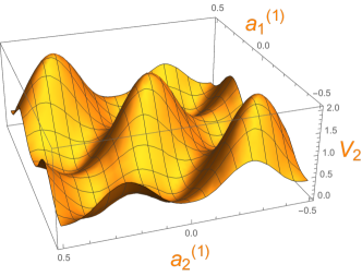
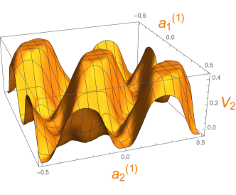
Figure 3: $V_{2}$ for $SU(3)$ conifold with cyclically identified holonomies: on the left we fixed $\Delta_{F_{1}}=0.12,\Delta_{F_{2}}=0.15,\Delta_{B}=0.22$ and we can observe that the function enjoys a local maximum at the origin; on the right we fixed $\Delta_{F_{1}}=0.05,\Delta_{F_{2}}=0.1,\Delta_{B}=0.3$ and we can observe that $V_{2}$ only possesses plateaux.

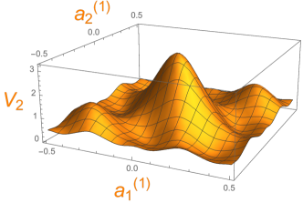
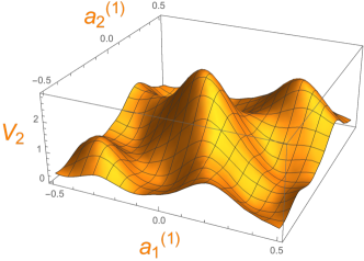
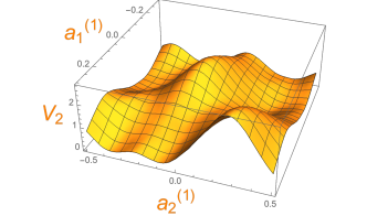
Figure 4: $V_{2}$ in the $a^{(1)}_{1}-a^{(1)}_{2}$ plane for $SU(4)$ conifold with cyclically identified holonomies and $\Delta_{F_{1}}=0.1,\Delta_{F_{2}}=0.15,\Delta_{B}=0.2$; from the top left in clockwise sense we fixed $a^{(1)}_{3}=0$, $a^{(1)}_{3}=0.08$ and $a^{(1)}_{3}=0.16$. We notice a minimum whose lowest value is reached for $a^{(1)}_{3}=0$.

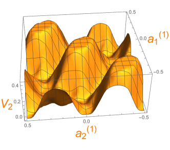
Figure 5: $V_{2}$ in the $a^{(1)}_{1}-a^{(1)}_{2}$ plane for $SU(4)$ conifold with cyclically identified holonomies and $\Delta_{F_{1}}=0.05,\Delta_{F_{2}}=0.1,\Delta_{B}=0.3\,,a^{(1)}_{3}\,=\,0$; only plateaux are present.

We can perform a similar analysis at rank 3. In this case we have three independent variables, $a^{(1)}_{1}$, $a^{(1)}_{2}$ and $a^{(1)}_{3}$ and thus we cannot make a single plot; we need to use a slightly different technique: we can make a plot $V_{2}$ in the $a^{(1)}_{1}-a^{(1)}_{2}$ plane at fixed $a^{(1)}_{3}$ and then vary the value of this last holonomy. If a minimum is located at the origin, $V_{2}$ restricted to the $a^{(1)}_{1}-a^{(1)}_{2}$ plane should have a minimum, as deep as we get closer to $a^{(1)}_{3}\,=\,0$. This is the kind of behaviour that we can observe in figure 4, where we fixed the fugacity in such a way the condition $\Delta_{F_{1}}+\Delta_{F_{2}}>\Delta_{B}$ to hold. When $\Delta_{F_{1}}+\Delta_{F_{2}}<\Delta_{B}$, instead, the presence of plateaux is already evident from a plot of $V_{2}$ at $a^{(1)}_{3}=0$, as shown in figure 5. Let us stress finally stress that, even relaxing the assumption (128), we can use other numerical tools such as FindMaximum/FindMinimum of Mathematica in order to understand the behaviour of $V_{2}$; this kind of study still returns the same results as before.