Storing and Querying Large-Scale Spatio-Temporal Graphs with High-Throughput Edge Insertions

Abstract

Real-world graphs often contain spatio-temporal information and evolve over time. Compared with static graphs, spatio-temporal graphs have very different characteristics, presenting more significant challenges in data volume, data velocity, and query processing. In this paper, we describe three representative applications to understand the features of spatio-temporal graphs. Based on the commonalities of the applications, we define a formal spatio-temporal graph model, where a graph consists of location vertices, object vertices, and event edges. Then we discuss a set of design goals to meet the requirements of the applications: (i) supporting up to 10 billion object vertices, 10 million location vertices, and 100 trillion edges in the graph, (ii) supporting up to 1 trillion new edges that are streamed in daily, and (iii) minimizing cross-machine communication for query processing. We propose and evaluate PAST, a framework for efficient PArtitioning and query processing of Spatio-Temporal graphs. Experimental results show that PAST successfully achieves the above goals. It improves query performance by orders of magnitude compared with state-of-the-art solutions, including JanusGraph, Greenplum, Spark and ST-Hadoop.

1 Introduction

Graphs have been widely used to represent real-world entities and relationships. Real-world graphs often contain spatio-temporal information generated by a wide range of hardware devices (e.g., sensors, POS machines, traffic cameras, barcode scanners) and software systems (e.g., web servers). We describe three representative application scenarios in the following.

Application 1: Customer Behavior Tracking and Mining

Understanding customer behaviors is helpful for detecting fraud and providing personalized services. For example, credit card companies track customers’ credit card uses for fraud detection. Internet companies track users’ browsing behaviors to achieve personalized recommendations. In a customer behavior tracking and mining application, people (customers) and locations can be modeled as graph vertices, while an edge linking a person vertex to a location vertex represents the event that the person visits the location at a certain time, as shown in Fig.fig. 1. This forms a spatio-temporal graph. People visiting similar locations at similar timestamps often have similar personal interests. In other words, it is desirable to discover groups of people vertices that have similar edge structures in the spatio-temporal graphs.

Figure 1: Customer behavior tracking and mining.

Application 2: Clone-Plate Car Detection

A clone-plate car displays a fake license plate that has the same license number as another car of the same make and model. In this way, the owner can avoid annual registration and insurance fees, and/or purchase the car without going through license plate lottery (which is a measure to address the traffic jam problems in major cities in China). However, it is difficult to detect a clone plate since a query to the car registration database will return a valid result. A promising approach is to exploit the large number of traffic cameras on high ways and local roads to detect clone plates. As a car passes by a traffic camera, the camera takes a photo and automatically recognizes the license number on the car plate. Car plates and cameras can be modeled as vertices in a spatio-temporal graph. An edge connecting a car plate vertex to a camera vertex indicates that the camera records the car plate at a certain time. Then, a clone plate is detected if a car plate vertex has two edges whose locations are far apart but timestamps are close such that it is impossible for the car to cover the distance in such a short period of time.

Application 3: Shipment Tracking

Recent years have seen rapid growth of the shipping business. E-commerce sites, such as Amazon and Alibaba, have become increasingly popular. Customers place orders online and the ordered goods are delivered to their door steps by shipping companies. Each shipment package contains a barcode. Shipping companies track packages by scanning the barcodes on packages with barcode scanners in regional or local offices. The problem of shipment tracking can be modeled as a spatio-temporal graph. Packages and barcode scanners are represented as vertices. The event that a barcode scanner detects a package is recorded as an edge between the package vertex and the scanner vertex. In this way, the spatio-temporal graph can be used to track shipment and answer status-checking queries.

Challenges for Storing and Querying Spatio-Temporal Graphs

Based on the commonalities of the three applications, we define a formal spatio-temporal graph model, where a graph consists of location vertices (e.g., locations, cameras, barcode scanners), object vertices (e.g., people, car plates, packages), and event edges that connect them. Compared with static graphs, spatio-temporal graphs pose more significant challenges in data volume, data velocity, and query processing:

• Data Volume: $\sim$10 billion object vertices, $\sim$10 million location vertices, and $\sim$100 trillion edges. First, the requirement of $\sim$10 billion object vertices is based on the fact that there are about 7.5 billion people in the world. Second, according to booking.com, there are about 1.9 million hotels and other accommodations in the world. Suppose there are 5 times more shops, restaurants, and theatres than hotels. Then the total number of locations can be on the order of 10 million. Finally, suppose an object vertex sees about 10 new edges per day. If we store the edges generated in the recent 3 years in the graph, there can be about 100 trillion edges in the graph. The data volume of a spatio-temporal graph can be much larger than static graphs.

• Data Velocity: up to 1 trillion new edges per day. Compared with static graphs, spatio-temporal graphs must support a large number of new edges per day. Suppose there are an average of 10 new edges per object vertex daily, and peak cases (e.g., Black Friday shopping) can see ten times more activities. This leads to a peak velocity of 100 new edges per object vertex daily, i.e. 1 trillion new edges in total per day.

• Query Processing: prohibitive communication cost. The data volume and velocity challenges entail a distributed solution that stores the graph data on a number of machines. However, without careful designs, processing queries can easily lead to significant cross-machine communication. For example, in order to find subgroups of people with similar interests (i.e. visiting similar locations at similar time), it is necessary to combine the spatial information in location vertices, the temporal information in edges, and properties of person vertices in the computation. As the data volume is huge, the cross-machine communication cost can be prohibitively high.

However, existing graph partitioning solutions [28, 4, 37, 44] focus mostly on static graphs, trying to minimize the number of cut edges across partitions and balance the partition sizes. Unfortunately, these solutions do not take into account spatio-temporal characteristics, which are important for query processing in spatio-temporal graphs. On the other hand, storing and querying spatio-temporal graphs using state-of-the-art distributed graph database systems (e.g., JanusGraph [21]), MPP relational database systems (e.g., Greenplum [16]), big data analytics systems (e.g., Spark [39]), or Hadoop enhanced for spatio-temporal data (i.e. ST-Hadoop [3]) result in poor performance (cf. Section section 8).

Our Solution: PAST

In this paper, we propose and evaluate PAST, a framework for efficient PArtitioning and query processing of Spatio-Temporal graphs. We propose diversified partitioning for location vertices, object vertices, and edges. We exploit the multiple replicas of edges to design spatio-temporal partitions and key-temporal partitions. Then we devise a high-throughput edge ingestion algorithm and optimize the processing of spatio-temporal graph queries. Experimental results show that PAST can successfully address the above challenges. It improves query performance by orders of magnitude compared to state-of-the-art solutions, including JanusGraph, Greenplum, Spark, and ST-Hadoop.

Contributions

The contributions of our work are threefold:

• We define a formal model for spatio-temporal graphs, and examine the design goals and challenges for storing and querying spatio-temporal graphs.

• We propose PAST, a framework for efficient PArtitioning and query processing of Spatio-Temporal graphs. It consists of a number of interesting features: (i) diversified partitioning for different vertex types and different edge replicas; (ii) graph storage with compression to reduce storage space consumption; (iii) a high-throughput graph ingestion algorithm to meet the challenge of data velocity; (iv) efficient query processing that leverages the different graph partitions; and (v) a cost model to choose the best graph partitions for query evaluation.

• We compare the efficiency of PAST with state-of-the-art solutions, including JanusGraph, GreenPlum, Spark, and ST-Hadoop in our experiments. We design a benchmark based on the query workload of the representative applications. Experimental results show that PAST achieves orders of magnitude better performance than state-of-the-art solutions.

Paper Organization

The remainder of the paper is organized as follows. Section section 2 reviews related literature. Section section 3 presents a formal definition of spatio-temporal graphs. Section section 4 overviews the system architecture of PAST. Section section 5 elaborates the partitioning and storage scheme for spatio-temporal graphs. Section section 6 describes the high-throughput edge ingestion support in PAST. Section section 7 presents optimizations on spatio-temporal query processing. Section section 8 presents experimental results. Section section 9 discusses several interesting issues. Finally, Section section 10 concludes the paper.

2 Related Work

We consider four solutions in the context of spatio-temporal graphs in Section section 2.1, and discuss more related work in Section section 2.2.

2.1 Supporting Spatio-Temporal Graphs with Existing Solutions

Distributed Graph Database Systems

Graph database systems (e.g., JanusGraph [21], Titan [43], Neo4j [30], SQLGraph [41], ZipG [24]) often support the property graph data model. We consider distributed graph database systems (e.g., JanusGraph [21], Titan [43]) for supporting spatio-temporal graphs. They store vertices and edges in Key-Value stores (e.g., Cassandra [8], HBase [18]) and exploit search platforms (e.g., Elasticsearch [12], Solr [38]) as indices for selective data accesses. Simple graph traversal queries can be efficiently handled. However, they are inefficient for large-scale spatio-temporal graphs because (i) they do not support direct filtering on time or spatial ranges, which are frequently used in spatio-temporal queries, and (ii) they need to scan the entire graph then invoke big data analytics systems (e.g., Spark [39]) for complex queries, which incurs huge I/O overhead.

MPP Relational Database Systems

We can store graph vertices and edges as relational tables in MPP database systems (e.g., Greenplum [16]), and use SQL for querying spatio-temporal graphs. Greenplum supports partitioning on multiple subsequent dimensions. The data is first partitioned by the first partition dimension. Then the second partition dimension is applied to each first-level partition to obtain a set of second-level partitions, so on and so forth. The partitions in all dimensions form a tree. MPP database systems can be inefficient for spatio-temporal graphs because (i) there is no support for spatial partitions, and (ii) any query has to start at the root-level and follow the tree even if the query does not have filtering predicates on the first partition dimension, potentially incurring significant CPU, disk I/O, and communication overhead.

Big-data Analytics Systems

General-purpose big-data analytics systems (e.g., Hadoop [17], Spark [39]) support large-scale computation on data stored in underlying storage systems, such as distributed file systems (e.g., HDFS), distributed key-value stores (e.g., Cassandra [8]). We can store the spatio-temporal graphs in the underlying storage systems, and run computation jobs on big-data analytics systems for querying spatio-temporal graphs. However, the system needs to load the entire graph before processing. It is not suitable for simple graph traversal queries. Since there is no support for filtering on time or spatial ranges on the underlying graph data, complex queries can see large unnecessary overhead due to reading the entire graph.

ST-Hadoop

ST-Hadoop [3] is an extension to Hadoop [17] and SpatialHadoop [13]. It represents previous studies that exploit multi-dimensional indices for supporting spatio-temporal data [31, 6, 34, 1, 26], and provides a scalable solution when data volume is large. ST-Hadoop organizes data into two-level indices. The first level is based on the temporal dimension, while the second level builds spatial indices. In this way, ST-Hadoop reduces data accessed for queries with temporal and spatial range predicates, thereby achieving better performance than Hadoop and SpatialHadoop. However, there are several disadvantages of ST-Hadoop for supporting spatio-temporal graphs. First, ST-Hadoop sacrifices storage for query performance. ST-Hadoop replicates its two-level indices into multiple layers with different temporal granularities (e.g., day, month, year). In each layer, the whole data set is replicated and partitioned. Second, ST-Hadoop is inefficient in supporting streaming data ingestion. It needs to sample across all data to estimate the data distribution and compute temporal and spatial boundaries. This basically requires temporarily storing incoming data and then periodically shuffles the data to build the indices. Depending on the temporal granularity, this may incur large temporal storage overhead and huge bursts of computation. Third, there is no support for indexing vertex IDs. Consequently, simple graph traversal queries may incur significant I/O overhead for reading a large amount of data. Finally, ST-Hadoop is based on the MapReduce framework, where the intermediate results are written to disks, potentially incurring significant disk I/O overhead.

2.2 Other Related Work

There are a large number of static graph partitioning algorithms in the literature, such as METIS [22], Chaco [4, 19], Scotch [32], PMRSB [5], ParMetis [23], Pt-Scotch [9]. Several recent studies introduce light-weight algorithms for partitioning large-scale dynamic graphs [20, 45, 40, 29]. However, none of these proposed methods leverage spatio-temporal characteristics of the data, which are important for query processing in spatio-temporal graphs.

Previous bipartite graph partitioning algorithms [10, 14] focus on simultaneous clustering with spectral co-clustering by computing eigenvalues and eigenvectors of Laplacian matrices. However, spatio-temporal graphs often have billions of vertices and trillions of edges, causing huge matrix storage and calculation overhead.

Time series databases (e.g., TimescaleDB [42], LittleTable [36]) enhance relational databases for supporting time-series data by partitioning rows by timestamp. In addition, every partition can be further sorted / partitioned by a specified key. However, there is no efficient support for spatial range predicates, which are important for spatio-temporal graphs.

Spatio-temporal graphs have been employed for video processing [25]. A video consists of a series of frames. Here, a graph vertex corresponds to a segmented region in a video frame. A spatial edge connects two adjacent regions in a frame, while a temporal edge links two corresponding regions in two consecutive frames. In this paper, we define a spatio-temporal graph model based on the representative applications. It is a bipartite graph, which is quite different from the model in the video processing context.

In our previous work, we proposed LogKV [7], a high-throughput, scalable, and reliable event log management system. The ingestion algorithm of PAST is an extension of the ingestion algorithm of LogKV. However, LogKV focuses mainly on temporal events. There is no support for spatial range predicates. Therefore, LogKV cannot efficiently process the spatio-temporal query workload considered in this paper. Moreover, a preliminary four-page version of this paper overviews the high-level ideas and shows preliminary experimental results [11].

3 Problem Formulation

In this section, we present the formal definition of spatio-temporal graphs and the query workload, then examine the design challenges.

3.1 Spatio-temporal Graph

Based on the representative applications in Section section 1, we define spatio-temporal graphs as follows:

Definition 1 (Spatio-temporal Graph)

A spatio-tem- poral graph $G=(V_{L},V_{O},E)$. $V_{L}$ is a finite set of location vertices. Every location vertex contains a location property. $V_{O}$ is a finite set of object vertices that represent objects being tracked. Every vertex in $V_{L}$ and $V_{O}$ is assigned a globally unique vertex ID. $E$ is a set of undirected edges. Every edge in $E$ connects an object vertex to a location vertex, and contains a time property.

Examples of location vertices include locations that customers visit in customer behavior tracking and mining, traffic cameras in clone-plate car detection, and barcode scanners in shipment tracking. Examples of object vertices include people in customer behavior tracking and mining, car plates in clone-plate car detection, and packages in shipment tracking. Every location vertex contains a location property such that given two location vertices $u$ and $v$, their distance $dist(u,v)$ is well defined. For example, if the application is concerned about geographic locations, then the location property consists of the latitude and longitude of the location vertex. An edge contains object ID, timestamp, location ID, and other application-dependent properties.

In essence, a spatio-temporal graph as defined in Definition 1 is an undirected bipartite graph. We do not consider edges between object vertices and edges between location vertices. This abstraction captures the key characteristics and the main challenges of the three representative applications.

3.2 Query Workload

We consider the following four types of queries based on the representative applications:

• Q1: object trace. Given an object and a time range, find the list of (object, timestamp, location)’s that represent the locations visited by the object during the time range. For example, Q1 can display the trace of a shipment package or the activities of a customer in a specified period of time.

• Q2: trace similarity. Given two objects and a time range, compute the similarity of the two object traces during the time range. Consider edge ($o1$, $t1$, $l1$) in object $o1$’s trace and edge ($o2$, $t2$, $l2$) in object $o2$’s trace. The two edges are considered similar if $|t2-t1|\leq TH_{time}$ and $dist(l2,l1)\leq TH_{dist}$, where $TH_{time}$ and $TH_{dist}$ are predefined thresholds on time and location distance, respectively. The similarity of the two traces is the count of similar edge pairs in the two traces.

• Q3: similar object discovery. Given an object $o$ and a time range, list the objects that have similar traces compared to $o$. Display the list in the descending order of trace similarity with $o$. Q3 can be used to discover people with similar interests in the customer behavior tracking and mining application.

• Q4: clone object detection. Given a time range, discover all the clone objects. An object $o$ is a clone object if there exists two incident edges ($o$, $t1$, $l1$) and ($o$, $t2$, $l2$) such that the computed velocity is beyond a predefined threshold: $\tfrac{dist(l2,l1)}{|t2-t1|}>TH_{velocity}$. Q4 supports clone-plate car detection. It can also be used to detect duplicate credit cards by a credit card company in the customer behavior tracking and mining application.

3.3 Understanding the Challenges

Data Volume

The goal is to support $\sim$10 billion object vertices, $\sim$10 million location vertices, and $\sim$100 trillion edges. Suppose the properties of a vertex require at most 100B. Then the object vertices and the location vertices require about 1TB and 1GB space, respectively. An edge contains at least (object ID, timestamp, location ID). Suppose each field takes 8B. Then an edge takes at least 24B. 100 trillion edges require 2.4PB space. The 3-replica redundancy policy requires a total 7.2PB storage space. Suppose the disk capacity of a machine is about 10TB. Therefore, 100 trillion edges require on the order of 1000 machines to store.

Data Velocity

The goal is to support up to 1 trillion new edges per day. This means 1Tx24B = 24TB/day of new ingestion data. A day consists of 86,400 seconds. Thus, this requires the design to support 290MB/s ingestion throughput.

Query Processing

We would like to minimize cross-machine communication in query processing. A random partition scheme would work poorly for Q1–Q4 because a large amount of unrelated data need to be visited. Since the four queries process time ranges, object IDs, and spatial locations, it is desirable to organize the data for efficient accesses using these dimensions.

4 PAST Overview

We propose PAST, a framework for efficient PArtitioning and query processing of Spatio-Temporal graphs. The system architecture of PAST is shown in Fig.fig. 2. PAST consists of multiple machines connected through the data center network in a data center. We assume that the latencies and bandwidths of the data center network are much better than those in wide area networks. There is a coordinator machine and a large number of (e.g., 1000) worker machines. The coordinator keeps track of meta information of the graph partitions and coordinates data ingestion. The workers store the graph data, handle incoming updates, and process queries.

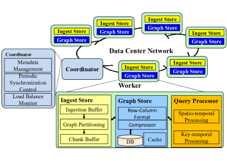
Figure 2: PAST system architecture.

Graph Partitioning and Storage

The GraphStore component in Fig.fig. 2 implements PAST’s graph partitioning methods and supports compressed storage of the main graph data. The GraphStore utilizes an underlying DB/storage system (e.g., the Cassandra key-value store in our implementation).

We propose diversified partitioning for location vertices and object vertices because they have drastically different characteristics. The number of location vertices is 1/1000 of that of object vertices. As the spatio-temporal graph is a bipartite graph, the average degree of a location vertex is 1000 times of that of an object vertex. As a result, they have very different impact on the communication patterns in query processing.

Edges consume much more space than vertices, and are often the performance critical factor in query processing. All four queries filter the edges with a given time range. Therefore, GraphStore should support time range filters efficiently. Q1, Q2, and Q4 access edges for a given object, two objects, and all objects, respectively. Hence, it would be nice to organize edges according to object IDs. On the other hand, Q3 can be more efficiently computed if edges are stored in spatio-temporal-aware orders so that GraphStore can filter out a large number of edges that are not relevant to the trace of the specified object. However, these requirements seem contradicting. We solve this problem by taking advantage of the multiple replicas of edges. For the purpose of fault tolerance, PAST stores multiple replicas for edges (e.g., 3 replicas). Therefore, we propose a spatio-temporal edge partition method and a key-temporal edge partition method for different edge replicas.

High-throughput Streaming Edge Ingestion

New edge updates are streamed in rapidly. As shown in Fig.fig. 2, the IngestStore component maintains a staging buffer for incoming new edges. All the worker machines handle incoming edges in rounds. They keep loosely synchronized clocks. In every round, the IngestStores collect the incoming edges in the current round. At the same time, IngestStores send edges collected in the previous round to their destination GraphStores based on the partitions computed by PAST’s partition methods. We design an efficient algorithm to perform the data ingestion that avoids hot spots in the data shuffling.

Query Processing and Optimization

Given PAST’s partition methods, we design a cost-based query optimizer to choose the best partitions for an input query. Our goal is to reduce cross-machine communication and edge data access as much as possible. The edge partitions divide the spatio-temporal space and key-temporal space into discretized blocks. We perform block-level filtering to avoid reading irrelevant edge data. Then we also take advantage of triangle inequalities for finer-grain filtering if geographic locations are used in the application.

5 Graph Partitioning and Storage

In this section, we describe the partitioning and storage methods for spatio-temporal graphs in PAST.

5.1 Diversified Partitioning

There are two main approaches to graph partitioning in the literature: vertex-based partitioning and edge-based partitioning. In vertex-based partitioning [22], a vertex is the basic partitioning unit. It assigns vertices along with their incident edges to partitions in order to minimize cross-partition edges. However, for a high-degree vertex, which is common in real-world graphs, there will be a large number of cross-partition edges no matter which partition to assign it. To address this problem, edge-based partitioning [15] assigns edges to partitions. If the incident edges of a (high-degree) vertex are in $k>1$ partitions, then the scheme chooses one partition to store the main copy of the vertex, and creates a ghost copy of the vertex in every other partition, thereby reducing the number of cross-partition edges to $k-1$ ghost-to-main virtual edges.

We propose diversified partitioning for spatio-temporal graphs. Our solution is inspired by edge-based partitioning. It considers the different properties of location vertices, object vertices, and edges, and the characteristics of spatio-temporal graph queries.

Location Vertex

The $\sim$10 million location vertices require about 1GB space (cf. Section section 3.3). A mid-range server machine today is often equipped with 100GB–1TB of main memory. Therefore, all the location vertices can easily fit into the main memory of one machine. On the other hand, location vertices are frequently visited for obtaining the locations of specified location IDs. Therefore, PAST stores all location vertices in every worker machine, and loads them into main memory at system initialization time. In this way, location information can be efficiently accessed locally without cross-machine communication. PAST updates all the worker machines when a location is updated. The update cost is insignificant because location vertices (e.g., shops, hotels, traffic camera locations, shipping services) change very slowly,

Object Vertex

PAST performs hash-based partitioning for object vertices. The scheme is inspired by Redis [35]. Each object vertex is assigned a unique 8-byte vertex ID. We first divide the vertices into slots. There are $2^{p}$ slots. Given a vertex ID $vid$, PAST computes $s=hash(vid)$, where $s\in[0,2^{p})$ is a $p$-bit slot ID. Then, we assign the slots to the worker nodes in a round robin manner: $w=i\bmod{N}$, where $N$ is the number of worker nodes. For fault tolerance purpose, we create 3 replicas by storing the slot to worker $w$, $w+1$, and $w+2$.

Edge

An edge contains a triplet (object ID, timestamp, location ID). Generally speaking, queries in spatio-temporal applications often contain filtering predicates on object IDs, time ranges, and locations. Specifically, Q1-Q4 all have time range filters. Q1, Q2, and Q4 will benefit from a data layout where edges of each object are stored together, while the amount of data accessed by Q3 is reduced if spatio-temporal filtering is efficiently supported. We take advantage of the multiple edge data replicas to design a twofold partitioning strategy as described in Section section 5.1.1 and section 5.1.2.

5.1.1 Skew-aware Spatio-temporal Edge Partitioning

Spatio-temporal edge partitioning first partitions edges according to the spatial dimension so that given an edge $(o,t,l)$, all edges associated with locations near $l$ are likely to be in the same partition. Then within a spatial partition, it constructs temporal sub-partitions, each of which contains edges in a disjoint time range. For the second part, it is straightforward to sort the edges by time and obtain the temporal sub-partitions. Therefore, we focus on the spatial partitioning part of the design in the following.

1

2

3Function UnboundedSpatioMapping(number of machines $M$, region list $\mathcal{R}$, location vertex list $V_{L}$)

4      

5      $\mathcal{R}_{z}$= Encode and sort regions in $\mathcal{R}$ by Z-codes;

6      foreach $r\in\mathcal{R}_{z}$ do Initialize weight $\mathcal{W}_{r}=0$;

7      

8      foreach $l\in V_{L}$ do  $r$ = $LocToRegion$($l$); $\mathcal{W}_{r}$++ ;

9      

10      $sum$=$0$; $rset$ = $\emptyset$;

11      foreach $r\in\mathcal{R}_{z}$ do

12            

13            $sum$+=$\mathcal{W}_{r}$; $rset$ = $rset\cup\{r\}$;

14            if $sum>=|V_{L}|/M$ then

15                   Assign $rset$ to the next machine;

16                  $sum$=$0$; $rset$ = $\emptyset$;

17            

18      

19      if $rset$ != $\emptyset$ then Assign $rset$ to the next machine;

20      

21

Algorithm 1 Unbounded weight-based spatial mapping.

1

2

3

4Function BoundedSpatioMapping( number of machines $M$, region list $\mathcal{R}$, location vertex list $V_{L}$, unit width $b$ )

5      

6      foreach $r\in\mathcal{R}$ do Region weight $\mathcal{W}_{r}=0$;

7      

8      foreach $l\in V_{L}$ do  $r$ = $LocToRegion$($l$); $\mathcal{W}_{r}$++ ;

9      

10      Suppose regions in $\mathcal{R}$ form a $h_{x}\times h_{y}$ 2D matrix. Group every $b\times b$ sub-matrix into a unit. The list of $\lceil\tfrac{h_{x}}{b}\rceil\times\lceil\tfrac{h_{y}}{b}\rceil$ units is denoted $\mathcal{U}$;

11      foreach $u\in\mathcal{U}$ do $\mathcal{UW}_{u}=\sum_{r\in u}\mathcal{W}_{r}$;

12      

13      $\mathcal{U}_{sorted}$ = sort $\mathcal{U}$ in descending $\mathcal{UW}_{u}$ order;

14      foreach $i$ do Machine weight $sum_{i}=0$;

15      

16      foreach $u\in\mathcal{U}_{sorted}$ do

17            

18            $i_{min}$ = ${\operatorname{argmin}}(sum_{i})$;

19            Assign $u$ to machine $i_{min}$;

20            $sum_{i_{min}}$ += $\mathcal{UW}_{u}$;

21      

22

Algorithm 2 Bounded weight-based spatial mapping.

We divide the universe of locations (e.g. the national map) into spatial partitions. We apply a grid to the universe. Each grid cell is a partition (a.k.a region). For simplicity, we consider square cells in this paper. The cell width is denoted as $a$. We choose $a$ such that (i) $a\gg D$, where $D=TH_{dist}$ is the distance threshold in Q2 and Q3, (ii) regions are small compared to the universe, and (iii) the number of regions are large compared to the number of worker machines. Constraint (i) ensures that distance similarity computation can be handled inside individual partitions in most cases. Constraint (ii) and (iii) make the partition size small enough so that multiple partitions can be assigned to a worker machine to achieve more balanced load.

Let partition $r$’s weight $\mathcal{W}_{r}$ be the number of locations in region $r$. The distribution of $\mathcal{W}_{r}$ can be very skewed. For example, there are usually more locations in regions with higher population. More object vertices (e.g., people) may visit such regions, leading to higher number of event edges. Therefore, we assume that $\mathcal{W}_{r}$ is proportional to the number of edges incident to location vertices in region $r$.

We would like to assign partitions to worker machines to achieve three goals: (i) ensure that $Weight_{i}=\sum_{r\in Worker_{i}}\mathcal{W}_{r}$ of worker machines are similar; (ii) ensure that adjacent partitions are on the same machine with large probability for reducing communication cost of evaluating spatial predicates; and (iii) enable multiple workers to evaluate a query in parallel for better performance.

In what follows, we propose an UnboundedSpatioMapping algorithm (Alg.1) that achieves the first two goals but fails for the third goal. Then we design a BoundedSpatioMapping algorithm (Alg.2), and compute the algorithm parameter $b$ for achieving the third goal.

Alg.1 lists the UnboundedSpatioMapping algorithm. To achieve goal (ii), it employs the Z-order curve. It sorts the regions by their Z-codes (Line 2), and assigns regions in contiguous Z-code intervals to machines (Line 5–10). In this way, neighboring regions are assigned to the same machine with large probability. Theorem 1 shows that the algorithm achieves goal (i).

Theorem 1

Suppose that $\mathcal{W}_{r}\leq\epsilon_{1}\tfrac{|V_{L}|}{M}$, where $\epsilon_{1}\ll 1$ and $\tfrac{|V_{L}|}{M}$ is the average load per worker machine. Given a target load skew $\epsilon_{2}$, then $\tfrac{sum_{i}}{|V_{L}|/M}-1<\epsilon_{2}$ (in Alg.1).

Proof 1

$\mathcal{W}_{r}\leq\epsilon_{1}\tfrac{|V_{L}|}{M}$ means that the weight of an individual region is much smaller than the average machine weight. This is guaranteed by constraints (ii) and (iii) for choosing $a$. Line 8 in Alg.1 ensures that the weight assigned to a worker machine $sum-W_{r}<\tfrac{|V_{L}|}{M}$. Thus, we have $sum_{i}<(1+\epsilon_{2})\tfrac{|V_{L}|}{M}$.

However, Alg.1 fails to achieve goal (iii). Consider the trace of an object $o$. $o$ may travel to a few cities. Those cities can be quite far away from each other, and visited locations may lie in an area $A$ (e.g., California), which contains a large number of partitions. However, Alg.1 may assign the entire $A$ to a single machine (e.g., our experiments use 10 worker machines). As a result, the partitions do not allow multiple workers to process the task in parallel.

Alg.2 solves the problem by assigning $b\times b$ adjacent spatial partitions to a worker at a time, where $b\geq 1$ is a control parameter. The solution is based on the observation that the locations inside a city are often in spatial partitions that are close to each other. With a larger $b$, it is more likely that locations in the same city of a trace are stored on the same machine, and therefore the amount of cross-machine communication may be reduced. However, when $b$ is too large, the number of workers that can process a single query are roughly equal to the number of cities that $o$ visits, which significantly limits the parallelism of query processing. Therefore, Alg.2 has to choose an appropriate $b$ to strike a balance between communication cost and parallelism.

Alg.2 works as follows. It computes the weight $\mathcal{W}_{r}$ of every region $r$ (Line 2–2). Then, it groups $b\times b$ adjacent regions into units (Line 2), and computes the weight $\mathcal{UW}_{u}$ of every unit, which is the sum of the weights of all the regions in this unit (Line 2). The algorithm assigns units to worker machines and balances the loads. To do this, it sorts the units in the descending order of unit weights (Line 2), then employs a greedy algorithm to always assign the next heaviest unit to the machine with the smallest load (Line 2–2).

We derive constraints on parameter $b$ to satisfy the above goals. Theorem 2 shows the condition to balance the load among all worker machines, and Theorem 3 shows the condition to balance communication cost and parallelism.

Combining Theorem 2 and Theorem 3 and the conditions for $b$, we have $\tfrac{D}{2a(1-\sqrt{\alpha^{\prime}})}\leq b\leq\sqrt{\epsilon_{2}/\epsilon_{1}}$, where $a\gg D$, $D=TH_{dist}$, $\epsilon_{1}\ll 1$ (e.g., $\epsilon$=0.001) and $\alpha^{\prime}=max(\alpha,\tfrac{(2a-D)^{2}}{4a^{2}})$.

Theorem 2

Suppose that $\mathcal{W}_{r}\leq\epsilon_{1}\tfrac{|V_{L}|}{M}$, where $\epsilon_{1}\ll 1$ and $\tfrac{|V_{L}|}{M}$ is the average load per worker machine. Given a target load skew $\epsilon_{2}$, if $b\leq\sqrt{\epsilon_{2}/\epsilon_{1}}$, then $\tfrac{sum_{i}}{|V_{L}|/M}-1<\epsilon_{2}$.

Proof 2

$\mathcal{W}_{r}\leq\epsilon_{1}\tfrac{|V_{L}|}{M}$ means that the weight of an individual region is much smaller than the average machine weight. This is guaranteed by constraints (ii) and (iii) for choosing $a$. The greedy algorithm ensures that the weight assigned to a worker machine $sum_{i}<\tfrac{|V_{L}|}{M}+max(\mathcal{UW}_{u})$. As each unit consists of $b^{2}$ regions, $max(\mathcal{UW}_{u})\leq b^{2}max(\mathcal{W}_{r})\leq b^{2}\epsilon_{1}\tfrac{|V_{L}|}{M}$. Combining the two inequalities and the condition for $b$, we have $sum_{i}<(1+\epsilon_{2})\tfrac{|V_{L}|}{M}$.

Theorem 3

Given a target probability $\alpha$, if $b\geq\tfrac{D}{2a(1-\sqrt{\alpha^{\prime}})}$, where $\alpha^{\prime}=max(\alpha,\tfrac{(2a-D)^{2}}{4a^{2}})$, then $\forall$ unit $\mathcal{U}$, location $l$ and $l_{nr}$: $Prob[l_{nr}\in\mathcal{U}|l\in\mathcal{U}\wedge dist(l_{nr},l)\leq D]\geq\alpha$.

Proof 5.1.

We divide a $ba\times ba$ unit (each unit is $b\times b$ adjacent spatial partitions, each partition is a cell with width $a$) into 9 parts, as illustrated in Fig.3a. $S_{1}$ is an inner square. $P[l_{nr}\notin U|l\in S_{1}]=0$. $S_{2}$ is a $(ba-2D)\times D$ rectangle. There is a single unit adjacent to $S_{2}$. We consider the four $S_{2}$ similarly. $P[l\in\cup S_{2}]=\tfrac{4(ba-2D)D}{(ba)^{2}}$. $S_{3}$ is a $D\times D$ square. There are three units (including the one in the diagonal position) adjacent to $S_{3}$. We also consider the four $S_{3}$ similarly. $P[l\in\cup S_{3}]=\tfrac{4D^{2}}{(ba)^{2}}$.

Figure 3: Dividing a unit into nine parts.

We derive bounds on the probability by using Chebyshev distance $dist_{c}(l_{1},l_{2})=max(|x_{1}-x_{2}|,|y_{1}-y_{2}|)$. Note that Euclidean distance $dist(l_{1},l_{2})\geq dist_{c}(l_{1},l_{2})$. Given a location in $S_{2}$ ($S_{3}$), Fig.3b (Fig.3c) illustrates the shadow area outside of the unit where its nearby location may reside in. We have

$\begin{array}[]{l}\par Prob[l_{nr}\notin\mathcal{U}|l\in\mathcal{U}\wedge dist(l_{nr},l)\leq D]\vspace{0.05in}\par\\ \par=Prob[l_{nr}\notin\mathcal{U}|l\in S_{2}]Prob[l\in\cup S_{2}]\vspace{0.05in}\par\\ \par+Prob[l_{nr}\notin\mathcal{U}|l\in S_{3}]Prob[l\in\cup S_{3}]\\ \vspace{-0.05in}\\ \par\leq\par\frac{\iint_{S_{2}}\frac{2Dy}{4D^{2}}dxdy}{(ba-2D)D}\frac{4(ba-2D)D}{(ba)^{2}}+\frac{\iint_{S_{3}}\frac{2Dx+2Dy-xy}{4D^{2}}dxdy}{D^{2}}\frac{4D^{2}}{(ba)^{2}}\vspace{0.08in}\par\\ \par=\frac{4baD-D^{2}}{4b^{2}a^{2}}\par\vspace{0.05in}\par\end{array}$

$\begin{array}[]{l}\par Prob[l_{nr}\in\mathcal{U}|l\in\mathcal{U}\wedge dist(l_{nr},l)\leq D]\vspace{0.05in}\par\\ \par=1-Prob[l_{nr}\notin\mathcal{U}|l\in\mathcal{U}\wedge dist(l_{nr},l)\leq D]\vspace{-0.05in}\par\\ \par=1-\frac{4baD-D^{2}}{4b^{2}a^{2}}\par\vspace{0.05in}\par\end{array}$

We see that if $1-\tfrac{4baD-D^{2}}{4b^{2}a^{2}}\geq\alpha$, then the target is achieved.

The valid solution to this inequality is $b\geq\frac{D}{2a(1-\sqrt{\alpha})}$, if $\alpha\in[\frac{(2a-D)^{2}}{4a^{2}},1)$. Thus, we have if $b\geq\tfrac{D}{2a(1-\sqrt{\alpha^{\prime}})}$, where $\alpha^{\prime}=max(\alpha,\tfrac{(2a-D)^{2}}{4a^{2}})$, then $\forall$ unit $\mathcal{U}$, location $l$ and $l_{nr}$: $Prob[l_{nr}\in\mathcal{U}|l\in\mathcal{U}\wedge dist(l_{nr},l)\leq D]\geq\alpha$.

5.1.2 Key-temporal Edge Partitioning

Key-temporal edge partitioning first constructs key partitions to store edges of objects in the same slot. It follows the partitioning method of object vertices to obtain the key partitions. That is, given an edge (object ID, timestamp, location ID), it uses object ID to compute the slot ID $s$ and then maps $s$ to worker $w$. Then within a key partition, it constructs temporal sub-partitions. Similar to spatio-temporal partitioning, it divides edges into disjoint time ranges, each of which constitutes a sub-partition.

5.2 Compressed Columnar Edge Store

In this section, we focus on the storage of edges in a worker machine node. GraphStore exploits existing storage / DB systems (e.g., Cassandra in our implementation) as the underlying DB to store edge data.

GraphStore organizes edge data into (row key, edge data) pairs, where the row key uniquely identifies a spatio-temporal / key-temporal sub-partition and the edge data contain compressed list of (object ID, timestamp, location ID, other edge properties) in the sub-partition. The row key is a concatenation of the following fields:

• node id: uniquely identifies the worker node;

• partitioning method: ‘A’ for spatio-temporal partitioning and ‘B’ for key-temporal partitioning;

• partition-specific id: region ID in spatio-temporal partitioning or slot ID in key-temporal partitioning;

• time range: TimeRange = $\lfloor\mbox{timestamp/TRU}\rfloor$, where TRU (Time Range Unit) is a configuration parameter used to discretize time.

For the edge data, we employ columnar layout for the attributes then compress the columns. Columnar layout is attractive because (i) it has good compression ratio and (ii) a query needs to uncompress and access only the relevant columns. For example, we put the object IDs of all edges in the sub-partition in an array, then compress the array. Similarly, we obtain the compressed representations of timestamps, location IDs, and other edge properties if exist. We measure the compression ratios and efficiency of several well-known compression algorithms, and choose LZ4 and Snappy in PAST because of their good performance [33].

To store the columns in Cassandra, we have two implementations: (i) C: we create multiple tables (or column families) in Cassandra, and store the compressed column of each edge attribute in a separate table; and (ii) R: we concatenates all the compressed columns into a single binary value, and store the value in a single Cassandra table. R essentially implements the PAX layout [2]. We evaluate the two implementations experimentally.

5.3 Fault Tolerance

PAST maintains edge replicas using different partitioning methods. However, this might cause two replicas of the same edge to reside in the same physical machine.

In our design, we check if such situation occurs and store the edge to another machine to ensure replicas are on different machines. Suppose an edge is assigned to worker $w_{s}$ in spatio-temporal partitioning, and to $w_{k}$ in key-temporal partitioning. The problem occurs if $w_{s}$=$w_{k}$. If the condition is true, then PAST will store a copy of the edge to worker $w_{s}+1$.

We compute the extra space required. Suppose that there are $M$ worker nodes. Edges are evenly distributed across the workers. Then the probability that an edge is assigned to a worker is $\tfrac{1}{M}$. The probability that $w_{s}$=$w_{k}$ is $M\cdot\tfrac{1}{M}\cdot\tfrac{1}{M}=\tfrac{1}{M}$. Therefore, the additional storage incurred is $\tfrac{1}{M}$ of the total edge data size. When $M$ is large (e.g., 100–1000), the extra space required is negligible.

6 High-Throughput Edge Ingestion

The data velocity challenge requires PAST to support up to 1 trillion new edges per day. We break down this goal into three sub-goals: (i) store up to 1 trillion new edges per day; (ii) achieve the proposed partitioning and storage strategy for the new edges as described in Section section 5; and (iii) balance the ingestion workload across the worker machines and avoid hot spots as much as possible. While directly reflecting the desired ingestion throughput, sub-goal (i) is not sufficient by itself. The other two sub-goals are important because sub-goal (ii) supports sustained ingestion performance and enables query processing on new edges, and sub-goal (iii) improves the scalability of the system.

We propose a high-throughput edge ingestion algorithm as described in Alg.algorithm 3, which extends our previous work on event log processing [7] to support diversified partitioning for spatio-temporal graphs. The high-level picture of the algorithm is as follows. IngestStore on each machine buffers the incoming new edges before shuffling them to GraphStore to implement the desired partitioning strategy. IngestStore employs double buffering. It buffers $m$-TRU worth of data while shuffling the previous $m$-TRU worth of data to GraphStore on the destination workers at the same time. $m$ is a parameter to tolerate instant ingestion bursts at individual IngestStores and avoid hot spots in shuffling.

Alg.algorithm 3 consists of three functions. The first function, IngestStore_AppendNewEdge, is invoked by IngestStore upon receiving a new edge. It appends the new edge to the end of inbuf (Line algorithm 3).

Every $m$-TRU time, the coordinator initiates a new round of shuffling operation by broadcasting a NextRound message with a $t_{start}$ parameter to all workers. Then IngestStore at each worker invokes the second function, IngestStore_ComputePartition, to compute the partitions for edges in $[t_{start},t_{start}+m\cdot\mbox{TRU})$ and copy the edges to outbuf. Note that the coordinator can initiate the round at time $t_{start}+m\cdot\mbox{TRU}+t_{delay}$ in order to tolerate communication delays from event sources for up to $t_{delay}$ time. The function computes the spatio-temporal partition (Line 7–9) and the key-temporal partition (Line 10–12) for an edge. Then it checks if the destination workers of the spatio-temporal and the key-temporal partitions collide. In such cases, it copies the edge to the outbuf of the next worker as discussed in Section section 5.3 (Line 15–16). In the end, the function truncates the inbuf. After the invocation, IngestStore replies a PartitionDone message to the coordinator. Note that the copy operation is very similar to the partitioning step in the in-memory partitioned hash join algorithm. When the number of destination workers is large, there can be significant TLB and cache misses. We perform multi-pass copying in the spirit of the radix-cluster algorithm [27] for better CPU cache performance.

When all the partitions are computed at all workers, the coordinator broadcasts a Shuffle message to all workers. Then GraphStore at each worker invokes the third function, GraphStore_Shuffle. It randomly permutes the worker list, then attempts to retrieve edges from IngestStore at every worker $w$ in the list $\mathcal{W}_{random}$ (Line 21–23). If $w$ is busy serving another GraphStore, then it puts $w$ into the busy list (Line 22). After processing $\mathcal{W}_{random}$, the function repeatedly processes workers in the busy list until the busy list is empty (Line 24–29). Upon receiving edge data from all workers, GraphStore sorts and compresses the edges, then stores the compressed data as described in Section section 5.2 (Line 30).

We re-examine the three sub-goals. It is clear that sub-goal (ii) is achieved by Ingest_StoreComputePartition and GraphStore_Shuffle. For sub-goal (iii), the double buffering mechanism and the random permutation are designed to reduce hot spots as much as possible. For sub-goal (i), we measure the ingestion throughput experimentally in Section section 8.

1

2

3Function IngestStore_AppendNewEdge(objId,time,locId)

4       Append edge (objId,time,locId) to inbuf;

5

6Function IngestStore_ComputePartition($t_{start}$, $m$, Worker list $\mathcal{W}=\{w_{0},\cdots,w_{n-1}\}$)

7      

8      foreach (objId,time,locId) $\in$ inbuf and

9                 time $\in[t_{start},t_{start}+m\cdot\mbox{TRU})$ do

10            

11            tr= time / TRU;

12                   /* Compute spatio-temporal partition */

13            $w_{s}$= $ComputeWorkerforLocation$(locId);

14            Append (objId,time,locId) to outbuf_s[$w_{s}$][tr];

15                   /* Compute key-temporal partition */

16            $w_{k}$= $ComputerWorkerforObj$(objId);

17            Append (objId,time,locId) to outbuf_k[$w_{k}$][tr];

18                   /* check if need extra replica for fault tolerance */

19            if $w_{s}$ == $w_{k}$ then

20                  

21                  $w_{next}$ = $GetNextWorker$($\mathcal{W}$, $w_{s}$);

22                  Append (objId,time,locId) to outbuf_f[$w_{next}$][tr];

23            

24      

25      Truncate inbuf to free the space of the processed edges;

26

27Function GraphStore_Shuffle($\mathcal{W}=\{w_{0},\cdots,w_{n-1}\}$)

28       $me$ = My worker Id;

29      $\mathcal{W}_{random}$ = Randomly permute the worker list $\mathcal{W}$;

30      foreach $w\in\mathcal{W}_{random}$ do

31             if Worker $w$ is busy then  Put $w$ into $busylist$;

32             else  Retrieve outbuf_s[$me$][..], outbuf_k[$me$][..], and outbuf_f[$me$][..] from worker $w$; ;

33            

34      

35      repeat

36             foreach $w\in busylist$ do

37                   if Worker $w$ is not busy then

38                         Retrieve outbuf_s[$me$][..], outbuf_k[$me$][..], and outbuf_f[$me$][..] from worker $w$;

39                        Remove $w$ from $busylist$;

40                  

41            

42      until  $busylist$ == $\emptyset$ ;

43      Compress and store received edges to the underlying DB;

44

Algorithm 3 High-throughput edge ingestion algorithm.

7 Spatio-temporal Graph Query
Processing and Optimization

Table 1: Terms used in the cost model.

$S_{e}$	edge size	$[t_{s},t_{e}]$	time range of a query
$R_{e}$	#edges ingested per second	$N_{q}$	#regions or #slots accessed by query
$N$	#regions or #slots in total	$P_{q}$	$P_{q}=N_{q}/N$
$c_{r}$	cost for reading from disk	$f$	network communication factor
$c_{a}$	cost for invoking backend	$p$	degree of parallelism
$\beta$	penalty factor $\beta\in$ (0,1)	$S_{T}$	edge data size in a TRU: $S_{e}R_{e}\cdot$ TRU
$N_{t}$	#TRU covered by a query’s time range: $\lceil{\tfrac{t_{e}}{TRU}}\rceil-\lceil{\tfrac{t_{s}}{TRU}}\rceil+1$

Table 2: Cost computation for Q1–Q4.

	spatio-temporal (ST)	key-temporal (KT)
Q1	$\tfrac{c_{r}S_{T}N_{t}+1048576c_{a}}{10\beta}$	$\tfrac{c_{r}S_{T}N_{t}+16384c_{a}}{16384\beta}$
Q2	$\tfrac{c_{r}S_{T}N_{t}+1048576c_{a}}{10\beta}$	$\tfrac{c_{r}S_{T}N_{t}+16384c_{a}}{16384\beta}$
Q3	$\tfrac{(c_{r}+f_{3})S_{T}N_{t}+1048576c_{a}}{10\beta}$	$\tfrac{(c_{r}+f_{3})S_{T}N_{t}+16384c_{a}}{10\beta}$
KT+ST	$\tfrac{c_{r}S_{T}N_{t}+16384c_{a}}{16384\beta}+\tfrac{(c_{r}+f_{sk3})S_{T}N_{t}x}{10485760\beta}+\tfrac{xc_{a}}{10\beta}$
Q4	$\tfrac{(c_{r}+f_{4})S_{T}N_{t}+1048576c_{a}}{10\beta}$	$\tfrac{c_{r}S_{T}N_{t}+16384c_{a}}{10\beta}$

Spatio-temporal query processing in PAST has two distinctive features compared to query processing in existing systems. First, there are two edge partitions: spatio-temporal and key-temporal. We study the cost models for choosing edge partitions in Section section 7.1. Second, there are predicates on edge similarity, which requires similarity joins on the spatial and/or temporal dimensions. We optimize the evaluation of edge similarity in Section section 7.2.

7.1 Cost-based Partition Selection

Query processing can exploit the two types of edge partitions to skip accessing a large amount of unrelated data and to reduce cross-machine communication overhead. In this subsection, we derive a cost model for the queries.

Table table 2 lists terms used in the model. Among the terms, $S_{e}$, $R_{e}$, $S_{T}$, $c_{r}$, and $c_{e}$ are constants. $N$ is the total number of regions (slots) in spatio-temporal (key-temporal) partitioning. For example, there are 16384 slots and 1048576 regions in our experiments. The time range parameters $t_{s}$, $t_{e}$, and $N_{t}$ are determined by a given query. $N_{q}$, $P_{q}$, $f$, and $p$ are dependent on both the given query and the chosen edge partition type.

The data size accessed by a query can be calculated as follows:

$$data\_size=S_{T}N_{t}P_{q}\vspace{-0.06in}$$

Then, we formulate the total cost for evaluating the query:

$$Cost =\tfrac{1}{\beta p}(Cost_{read}+Cost_{invoke}+Cost_{shuffle})$$

$$=\tfrac{1}{\beta p}[(c_{r}+f)S_{T}N_{t}P_{q}+c_{a}N_{q}]$$

where $\beta$ is a penalty factor. The actual degree of parallelism is $\beta p$.

$Cost_{read}$ is the cost of reading $data\_size$ amount of data from disk: $Cost_{read}=c_{r}data\_size$. $Cost_{invoke}$ is the cost of invoking the underlying DB. PAST retrieves all $N_{t}$ sub-partitions of every region / slot with a single invocation. Therefore, the number of invocations is $N_{q}$, and $Cost_{invoke}=c_{a}N_{q}$. $Cost_{shuffle}$ is the cost of communicating a fraction of the retrieved data across machines. $Cost_{shuffle}=f\cdot data\_size$. Here, parameter $f$ depends on the query evaluation strategy and the network bandwidth.

Given the cost model, we compute the cost of processing Q1–Q4 using different partitions. Table table 2 summarizes the computed costs. We set $N$ to be 1048576 and 16384 for spatio-temporal and key-temporal partitions, respectively. The degree of parallelism ($p$), the network communication factor ($f$) and region/slot proportion ($P_{q}$) differ as different partitions are selected for query execution. There are 10 workers in our experiments. Therefore, $p\leq 10$.

Q1: object trace

(i) spatio-temporal: Since the given object $o$ may visit any spatial locations during the time range, every worker reads its own spatio-temporal partition to look for edges that contain object $o$. Every region needs to be examined. No edge data shuffle is necessary. So $p=10,f=0,N_{q}=1048576,P_{q}=1$.

(ii) key-temporal: Only the worker that contains the key-temporal partition of $o$ reads the $o$’s slot. There is no data shuffling during computation. So $p=1,f=0,N_{q}=1,P_{q}=\tfrac{1}{16384}$.

Q2: trace similarity

(i) spatio-temporal: Compared with Q1, the query processing strategy is unchanged. Now every worker looks for edges that contain either given objects. So the parameters are also unchanged. $p=10,f=0,N_{q}=1048576,P_{q}=1$.

(ii) key-temporal: We perform Q1 then computed similarity between the obtained traces. In the worst case, the key-temporal partitions of the two given objects reside in two machines. So $p=2,f=0,N_{q}=2,P_{q}=\tfrac{1}{8192}$.

Q3: similar object discovery

Q3 is a heavy-weight query. Both the spatio-temporal and the key-temporal solutions read all data in the time range. Then they perform a join and a groupby operation by shuffling all the retrieved data among workers. Therefore, the network communication factor ($f_{3}$) is very large. (i) spatio-temporal: $p=10,N_{q}=1048576,P_{q}=1$. (ii) key-temporal: $p=10,N_{q}=16384,P_{q}=1$.

We design an optimized execution strategy for Q3 that combines the two partitions. (iii) key-temporal+spatio-temporal: It first obtains the trace of the given object $o$ by Q1 accessing the key-temporal partitions. Then it finds all locations visited by $o$, computes the regions from the locations, and sends the locations to workers that store the relevant regions. After that, each worker reads the relevant regions from its spatial-temporal partition and looks for edges that are similar to $o$’s trace. Finally, similar edges are grouped by objects to compute the aggregate similarities, which are then sorted to obtain the query result. While the final step performs data shuffling, the amount of data shuffled is reasonably small compared to that in (i) and (ii). Therefore, the network communication factor $f_{sk3}\ll f_{3}$. Suppose the number of regions to access is $x$ ($x\ll 1048576$), and all workers participate in the computation. So $p=10,N_{q}=x,P_{q}=\tfrac{x}{1048576}$.

Q4: clone object detection

(i) spatio-temporal: All machines participate in computation. They have to shuffle all the data in the time range. Suppose the network communication factor is $f_{4}$. Then $f_{4}\approx f_{3}$ for the same time range. Other parameters are $p=10,N_{q}=1048576,P_{q}=1$.

(ii) key-temporal: Each machine reads every slot in the time range. Since all edges of an object are in the same slot, velocity computation can be performed locally without data shuffling. Thus, $f=0,p=10,N_{q}=16384,P_{q}=1$.

Comparison

From Table table 2, we see that for Q1, Q2, and Q4, KT’s cost is lower than ST’s cost: $Cost_{KT}<Cost_{ST}$. Therefore, KT is the better partition to use. For Q3, $Cost_{ST+KT}<Cost_{KT}<Cost_{ST}$. Therefore, ST+KT should be selected.

In general, for a given query, we can apply the above analysis to compute the cost for different partition types, and choose the best partition or partition combination based on the computed costs.

7.2 Edge Similarity Computation

Optimizing Location Computation

We would like to improve the efficiency of computing $dist(l_{1},l_{2})\leq TH_{dist}$. The basic idea is to filter out far-away locations that cannot satisfy the inequality without computing the distance.

Given a set of locations in an area (e.g., a region or a unit). We apply a grid to the area, where a grid cell is a $\eta\times\eta$ square and $\eta\ll$ region width $a$. It is easy to convert the coordinates $(x,y)$ of a location $l$ into grid coordinates $(x_{g},y_{g})$: $x_{g}=\lfloor x/\eta\rfloor$, $y_{g}=\lfloor y/\eta\rfloor$. For $l_{1}(x_{1},y_{1})$ and $l_{2}(x_{2},y_{2})$, their grid coordinates are $(x_{g1},y_{g1})$ and $(x_{g2},y_{g2})$, respectively.

Let $d_{x}=|x_{2}-x_{1}|$, $d_{y}=|y_{2}-y_{1}|$, $d_{gx}=|x_{g2}-x_{g1}|$, and $d_{gy}=|y_{g2}-y_{g1}|$. Therefore, $d_{x}\in((d_{gx}-1)\eta,(d_{gx}+1)\eta)$ and $d_{y}\in((d_{gy}-1)\eta,(d_{gy}+1)\eta)$. According to triangle inequality, we have the following:

$$|d_{x}-d_{y}|<=dist(l_{1},l_{2})<=d_{x}+d_{y}\vspace{-0.05in}$$

Thus

$$(|d_{gx}-d_{gy}|-2)\eta<=dist(l_{1},l_{2})<=(d_{gx}+d_{gy}+2)\eta\vspace{-0.05in}$$

We use the above inequalities to calculate the lower bound of the distance between two locations. If the lower bound is larger than $TH_{dist}$, then we can avoid computing the actual distance, thereby reducing computation overhead.

Optimizing Time Computation

A sub-partition contains events in a TRU. For $|t_{2}-t_{1}|\leq TH_{time}$ computation, we can use the sub-partition row key (which encode the time range) to reduce data access and computation overhead. Let $d_{T}=\lceil TH_{time}/\mbox{TRU}\rceil$. If $t_{1}$ is in time range $tr_{1}$, we only need to consider $2d_{T}+1$ sub-partitions with time ranges in $[tr_{1}-d_{T},tr_{1}+d_{T}]$. In particular, when $TH_{time}<$ TRU, we only need to consider three sub-partitions with time ranges $tr_{1}-1$, $tr_{1}$, and $tr_{1}+1$.

8 Experimental Evaluation

In this section, we evaluate the performance of PAST. We would like to answer the following questions in the experiments:

• Can PAST efficiently support high-throughput edge insertions while achieving the desired graph partitions?

• What are the benefits of the proposed techniques, such as the diversified partition strategy, cost-based edge partition selection, compressed edge storage, and computation optimization?

• How does PAST compare to state-of-the-art systems (e.g., JanusGraph, Greenplum, Spark, and ST-Hadoop)?

8.1 Experimental Setup

Machine Configuration

The experiments are performed on a cluster of 11 machines. Each machine is a Dell PowerEdge blade server equipped with two Intel(R) Xeon(R) E5-2650 v3 2.30 GHz CPUs (10 cores/20 threads, 25.6MB cache), 128GB memory, a 1TB HDD and a 180GB SSD, running 64-bit Ubuntu 16.04 LTS with 4.4.0-112-generic Linux kernel. The blade servers are connected through a 10Gbps Ethernet. We use Oracle Java 1.8, Cassandra 2.1.9, JanusGraph 0.2.1, Greenplum 5.9.0, Spark 2.2.0, ST-Hadoop 1.2 and Hadoop 2.8.1 in our experiments.

Workload Generation

We generate a synthetic data set of customer shopping events. The goal to support 10 billion object vertices and 10 million location vertices are designed for clusters with 1000 machines. Given the machine cluster size in our experiments, we scale down the number of vertices by a factor of 100. Therefore, we would like to generate 100 million object vertices and 100 thousand location vertices.

First, we crawled 450 thousand hotel locations in China from ctrip.com (a popular travel booking web site in China). The locations are distributed across about 1100 areas (cities / counties / districts). We randomly choose 100 thousand locations from the real-world hotel locations as shopping locations. Second, we generate 100 million customers. As the number of shopping locations and the population of an area are often correlated, we assign customers to areas so that the number of customers is proportional to the number of locations in an area. Third, we would like to generate a data set that covers a 2-3 year period and can be stored in the cluster in the experiments. We assume 40% people are frequent shoppers and 60% people are infrequent shoppers. A frequent shopper and an infrequent shopper visit a randomly chosen shopping location in his or her area every week with probability 0.8 and 0.2, respectively. Edge timestamps are used to compute edge partitions and evaluate queries in our experiments. (Note that the week period is necessary to reduce the total data volume to fit into the cluster storage capacity. Our ingestion experiments will send the edge data as fast as possible to saturate the system disregarding edge timestamps). Finally, we produce a small number of cloned objects that visit shopping locations in far-away areas. The resulting graph contains 57 billion edges, which cover 800 days.

Parameter Settings

In spatio-temporal partitioning, we apply a $1024\times 1024$ grid to the map, obtaining 1048576 regions. Note that there are more hotels in the city than in the countryside. We see that hotels concentrate in 8660 regions. In key-temporal partitioning, we generate 16384 slots. We set TRU to be 24 hours.

We evaluate Q1-Q4 as described in Section section 3.2. By default, we set $TH_{time}=7h$, $TH_{dist}=100m$, $TH_{velocity}=120km/h$.

State-of-the-art Systems to Compare

We evaluate our proposed solution, PAST, and four state-of-the-art systems in the experiments:

• PAST (our proposed solution). We implement PAST in Java. The GraphStore uses Cassandra as the underlying DB backend and stores data on the HDDs. We customize Cassandra’s partitioner to manage the key-to-node mapping.

• JanusGraph (a state-of-the-art distributed graph store). A spatio-temporal graph is stored as a property graph. We choose Cassandra as JanusGraph’s storage backend. To facilitate edge retrieval for a given object (location) vertex, we set the vertex ID to be the object ID (location ID).

• Greenplum (a state-of-the-art MPP relational DB). Graph data is stored as relational tables in Greenplum. To minimize disk space usage, we create two tables for edge data and for location details with latitude and longitude, respectively. The two tables are linked by location ID. Q2, Q3 and Q4 perform join operations. We employ multi-dimensional partitioning for improving query performance. Vertex ID is the first dimension, and time is the second dimension.

• Spark+Cassandra (a state-of-the-art big-data analytics system). Graph data is stored in Cassandra. Spark loads the location data into memory at the beginning of execution to reduce the overhead of looking up locations. The loading time is less than 1 second, and is negligible compared with the query execution time. Spark accesses data in Cassandra for query processing, and saves the query results to HDFS.

• ST-Hadoop+Spark (a big data system specially optimized for spatio-temporal data). Given the TRU setting in PAST, we set ST-Hadoop’s partition granularity to be day. PAST’s spatio-temporal partitioning employs the Z-order curve. Therefore, we set ST-Hadoop’s spatial index technique to be the Z-order curve. To avoid MapReduce’s overhead of storing intermediate data to disks, we use Spark to read spatio-temporally indexed data in ST-Hadoop and compute the queries in memory.

(a)

(b)

Figure 4: Ingestion throughput seen at IngestStore and GraphStore evolving over time (#workers=10).

8.2 New Edge Ingestion

In this section, we measure the sustained edge ingestion throughput in PAST, and examine the distribution of data across workers.

As described in Section section 6, PAST shuffles $m$-TRU worth of data in every round. In our experiments, we set $m$ to be the number of worker machines. Note that edges are partitioned during ingestion.

Figure 5: Ingestion throughput varying the number of workers.

Edge Ingestion Throughput and Scalability

The edge ingestion throughput is the number of new edges streamed into all the GraphStores per second. We send edges in the data set as fast as possible in this set of experiments. We observe that the ingestion throughput stabilizes in the third round, as shown in Fig.fig. 4. Given this, we measure the ingestion throughput in the fifth and sixth rounds at IngestStores, and report the aggregate ingestion throughput as the sustained throughput in Fig.fig. 5.

In Fig.fig. 5, we vary the number of worker machines on the X-axis from 1 to 10 to study the scalability of our solution. The Y-axis reports the sustained ingestion throughput in million edges per second. From the figure, we see that the sustained ingestion throughput increases nearly linearly as the number of worker grows. The PAST design achieves good scalability for new edge ingestion.

Every worker in PAST can support an additional 0.85 million new edges per second. An edge takes 24 bytes in this experiment. Every worker in PAST can support additional 20MB/s ingestion bandwidth. Therefore, the design goal of 1 trillion new edges per day (or 290MB/s) for a full-scale spatio-temporal graph can be achieved with about 15 worker machines. This gives a lower bound of the actual number of nodes in a design, whose choice must also consider the performance of query processing.

Edge Ingestion Throughput Evolving Over Time

We measure the number of ingested edges seen by both IngestStores and GraphStores at every minute for about 50 minutes. Fig.fig. 4 shows the average per-machine throughput across all machines. The X-axis is wall-clock time. The Y-axis is the ingestion throughput in million edges per second. The error bars show the standard errors.

The upper figure in Fig.fig. 4 shows the ingestion throughput seen by IngestStores. IngestStores begin to handle incoming edges at time 0. The ingestion throughput quickly increases at the beginning. Then it fluctuates around 0.85 million new edges per second.

The lower figure in Fig.fig. 4 shows the ingestion throughput seen by GraphStores. GraphStores begin to receive data at time=360s. Its throughput reaches the peak with nearly 108MB/s (4.5 million edges per second) at time=480s. This is because Cassandra starts with empty in-memory buffers for receiving data, and the cost of storing to Cassandra is very low at the beginning. As time goes by, Cassandra moves into more steady states. The peak throughput reduces to 86MB/s (3.6 million edges per second) at the second round. The peak throughput in stable rounds (i.e. round 3 and beyond) is about 48MB/s (2.0 million events/s).

Note that IngestStores send both key-temporal data and spatio-temporal data. The shuffled data is essentially twice the amount of the incoming edge data. Therefore, the ingestion throughput seen at GraphStores is roughly twice as much as that seen at IngestStores.

Data Distribution

We would like to understand how well our partitioning methods work in terms of data distribution across machines. We measure the data size in each worker for both spatio-temporal edge partitions and key-temporal edge partitions. In Fig.fig. 6, the X-axis shows each worker machine, while the Y-axis reports data size in GB. From the figure, we see that PAST’s partitioning methods achieve balanced data distribution. Note that the data size of spatio-temporal partitions is roughly twice as large as the data size of key-temporal partitions. This is because PAST stores three replicas for edge data, of which two in spatio-temporal partitions, and one in key-temporal partitions.

Figure 6: Data distribution in different edge partitions.

8.3 Proposed Features in PAST

In this section, we evaluate the proposed features in PAST, including storage format, edge partition selection, computation optimization, and the spatial mapping algorithms.

8.3.1 Comparison of Two Storage Formats

We evaluate the two storage formats as described in Section section 5.2: (i) $C$: this is the baseline design, where edge properties are stored in separate tables (column families) with compression; and (ii) $R$: this is the PAX design, where the compressed columns are concatenated to store in a single table (column family). Since they both store compressed column data, $C$ and $R$ consume the same amount of disk space. However, their query performance can be different.

Figure 7: Effect of storage format for Q4.

Fig.fig. 7 reports query execution time for Q4 while varying the number of edge properties. Note that Q4 uses only three edge properties (i.e., object ID, timestamp, location ID) in computation. We perform the experiment on a single machine. The X-axis shows the total number of edge properties, and the Y-axis is elapsed time.

From the figure, we see that the cost of decompression is negligible. When there are three edge properties, $C$ and $R$ take nearly the same time for reading data from Cassandra because they retrieve the same amount of data from disk. However, as the number of properties increases beyond three, the query performance of $R$ deteriorates. The read time in $R$ increases as the number of properties increases. This is because $C$ avoids accessing irrelevant properties, while $R$ has to retrieve all properties.

8.3.2 Benefits of Cost-Based Edge Partition Selection

We perform a set of experiments to validate the analysis in Section section 7.1. Here, we evaluate Q1, which represents simple graph traversal queries, and Q3, which represents complex queries, using different edge partitions. The query time range is one day.

Table table 3 lists the execution time and accessed data size for Q1 and Q3 using the following solutions. (i) ST: a query accesses only spatio-temporal partitions. (ii) KT: a query accesses only key-temporal partitions. (iii) KT+ST for Q3: the optimized execution strategy for Q3, where PAST first accesses key-temporal partitions for retrieving the trace of the given object $o$, then accesses spatio-temporal partitions for computing objects that are similar to $o$.

From Table table 3, we see that for Q1, $Cost_{KT}<Cost_{ST}$, and for Q3, $Cost_{ST+KT}<Cost_{KT}<Cost_{ST}$. This observation is in accordance with the analysis based on the cost model in Section section 7.1. Overall, the best execution plans for Q1 and Q3 achieve a factor of 39.5x and 9.7x improvements over the second best plans.

Table 3: Query performance using different edge partitions.

	Q1		Q3
replica	size (MB)	time (s)	size (MB)	time (s)
KT	0.058	0.47	950	343.92
ST	950	18.57	950	636.52
KT+ST	–	–	9	35.63
Note: only Q3 can be optimized using both two edge partitions.

8.3.3 Benefits of Computation Optimization

We study the effect of optimization techniques for evaluating edge similarity, as described in Section section 7.2. We measure Q3’s execution time while varying the query time range from 1 day to 512 days. We compare three solutions: (i) ST-OP: the baseline implementation in PAST with both location and time computation optimized; (ii) T-OP: only time computation is optimized; (iii) NOP: there is no computation optimization.

Table 4: Query results varying time range for Q3.

#day	1	2	4	8	16	32	64	128	256	512
read(MB)	9	34	34	89	221	456	963	2000	4005	8134
#result($\times 10^{3}$)	3	7	7	13	27	45	87	174	333	566

Figure 8: Effect of algorithm optimizations for Q3.

Fig.fig. 8 reports query execution time in the logarithmic scale. Table table 4 lists the read data size and the number of query results for all the experiments in Fig.fig. 8. When the query time range is less than 4 days, the three solutions take nearly the same time. As the query time range increases, the performance difference becomes obvious. Overall, ST-OP outperforms T-OP and N-OP by a factor of up to 3.1x and 12.8x. The computation optimization is quite significant.

8.3.4 Effect of Spatial Mapping for Skewed Data

(a) Workload distribution

(b) Runtime

Figure 9: Effect of skew spatial data partitioning for Q3.

We compare unbounded spatial mapping (Alg.algorithm 1) and bounded spatial mapping (Alg.algorithm 2) using Q3. We consider three choices of b (i.e., 8, 4, and 2) for Alg.algorithm 2. According to Theorem 2, the corresponding lower bound of SF (spatial factor) is 88%, 77% and 56%, respectively. (we set region width $a$ to be $D$). The unbounded algorithm is labeled by $b=\infty$. PAST employs the optimized execution plan for Q3 as described in Section section 7.1.

Fig.fig. 9a shows the distribution of accessed regions for each machine when the query time range is 512 days. The smaller the SF is, the more machines are likely to contain regions used in the query. However, we would like to choose $b$ such that $b$ is not very small and data locality is maintained for most location computation. Fig.fig. 9b shows the execution time for $b=8$ and $b=\infty$. We see that the bounded algorithm achieves a small improvement of 10% over the unbounded algorithm.

8.4 Comparison with State-of-the-art Systems

We compare PAST with state-of-the-art systems, including JanusGraph, Greenplum, Cassandra+Spark, and ST-Hadoop+Spark. We are interested in two aspects: (i) storage space consumption and (ii) query performance.

8.4.1 Storage Space

Table table 5 shows storage space used in all systems. Note that PAST and Cassandra keep 3 replicas, and Greenplum stores 2 replicas by default. Due to disk space limitation, JanusGraph, Greenplum, and ST-Hadoop stores only 1 replica.

Table 5: Disk Space Consumption

	PAST	JanusGraph	Greenplum	Cassandra	ST-Hadoop
size (TB)	1.9	3.4	2.8	3.2	3.1
#replica	3	1	2	3	1

$\begin{array}[]{c}\includegraphics[width=433.62pt]{./pics/legend-eps-converted-to.pdf}\\ \begin{array}[]{cccc}\includegraphics[width=115.63243pt]{./pics/comparison-sel-q1-eps-converted-to.pdf}&\includegraphics[width=115.63243pt]{./pics/comparison-sel-q2-eps-converted-to.pdf}&\includegraphics[width=115.63243pt]{./pics/comparison-sel-q3-eps-converted-to.pdf}&\includegraphics[width=115.63243pt]{./pics/comparison-sel-q4-eps-converted-to.pdf}\par\end{array}\end{array}$

Figure 10: Query performance comparison ($TH_{time}$ = 7h, $TH_{dist}$ = 100m).

From the table, we see that compared with Cassandra, PAST achieves a factor of 1.7x space savings. PAST consumes less space than the other systems even if they store fewer number of replicas. If we calculate the space consumption for JanusGraph, GreenPlum, and ST-Hadoop to account for three replicas, then PAST reduces the space consumption of JanusGraph, GreenPlum, and ST-Hadoop by a factor of 5.4x, 2.2x, and 4.9x, respectively.

Note that JanusGraph stores the graph data in Cassandra. Both Cassandra and JanusGraph employ LZ4 compression. In comparison, PAST achieves much better space consumption. This is because PAST utilizes columnar layout for all edges in a sub-partition, and compresses the columnar edge properties. JanusGraph consumes more space than Cassandra because it stores each edge twice at both the incoming vertex and the outgoing vertex. PAST and Cassandra take less space to store one replica than Greenplum because of compression.

8.4.2 Query Performance

Fig.fig. 10 and Fig.fig. 11 compare the query performance for all systems, while varying the query time range and the threshold values, i.e. $TH_{time}$ and $TH_{dist}$. The Y-axis is executing time in the logarithmic scale. We do not run Q3 and Q4 on JanusGraph as it mainly focuses on simple traversal queries and employs Spark for complex queries. Therefore, Q3 and Q4 on JanusGraph can be represented by Q3 and Q4 on Cassandra+Spark, respectively.

There are several missing points in Fig.fig. 10(c) and (d). The experiments corresponding to the missing points run over one day and have not completed. Cassandra+Spark and ST-Hadoop+Spark are overwhelmed by shuffling for Q3 and Q4 with large query time ranges. For Q4, most systems compute the velocity of edges of an object in sorted time order. In contrast, in GreenPlum, the SQL query for Q4 would read and join all data for computing velocity, which quickly overwhelm the system.

$\begin{array}[]{c}\includegraphics[width=216.81pt]{./pics/legend2-eps-converted-to.pdf}\\ \begin{array}[]{cc}\includegraphics[width=101.17755pt]{./pics/q2-time10-space1000-eps-converted-to.pdf}&\includegraphics[width=101.17755pt]{./pics/q3-time10-space1000-eps-converted-to.pdf}\\ \end{array}\end{array}$

Figure 11: Query performance comparison ($TH_{time}$ = 10h, $TH_{dist}$ = 1000m).

From Fig.fig. 10 and Fig.fig. 11, we see that PAST achieves 1–4 orders of magnitude better performance compared with the four existing solutions. The partition and query processing schemes in PAST can effectively reduce the amount of data accessed from the underlying storage and the data communication cost. The main bottleneck of Cassandra+Spark is the disk I/Os for scanning all data. ST-Hadoop+Spark performs better than Cassandra+Spark because it exploits the spatio-temporal index to reduce the amount of data to read. However, as the query time range increases, ST-Hadoop+Spark’s performance degrades and approaches that of Cassandra+Spark. Greenplum achieves significantly better performance than ST-Hadoop+Spark for the simple queries, Q1 and Q2. This is because Greenplum first partitions by object then further sub-partitions by time. The object partitions fit the needs of Q1 and Q2 well. In contrast, there is no object indexing support in ST-Hadoop.

9 Discussion

Medium-grain Partitions for Object Vertices

Our partitioning scheme for object vertices is based on hash partitioning. However, if we know more about the object vertices, we may design better partitioning schemes. Note that too fine grained partitions result in the difficulty in recording the partitions and the significant expense in computing the partitions. Therefore, we consider medium-grain partitioning based on groups of vertices. We can add a group property to every vertex to record the group of the vertex. Then the partition decision is based on groups rather than every vertex. The group to machine assignment can be captured in the coordinator node, who also keeps track of the group statistics. The assignment of vertices to groups is application dependent. For example, it would be nice if people with similar behaviors are assigned to the same group.

Dynamic Vertex Group Partitions

Every worker node periodically reports group statistics to the coordinator machine. Based on the statistics, the coordinator machine computes the average (space and computation) loads per worker machine. It will ask worker nodes to migrate vertex groups if the load of a machine is beyond a threshold (e.g., +/- 5% of the average). The vertex groups to be migrated can be computed based on the collected statistics.

Alternative Implementation as Index on RDBMSs

We present a stand-alone implementation of PAST in this paper. Alternatively, we can implement PAST as a spatio-temporal index structure on top of RDBMSs. Then PAST can be applied to more applications that combine both spatio-temporal graphs and traditional relational data. PAST speeds up the part of queries that involve spatio-temporal graphs and returns a list of vertex IDs or edge IDs. Then the list can be combined with query outputs from relational queries to further compute the final query results.

More Extended Applications

The idea of PAST can be applied to slove more generalized multi-dimension graph problems, not limited by spatio-temporal dimension. Moreover, the concepts of space can be generalized as user space, commodity space, etc, and in the meanwhile, the distance can not only be Euclidean distance but also other similarity measurement.

10 Conclusion

In conclusion, we define a bipartite graph model for spatio-temporal graphs based on the commonalities of representative real-world applications, i.e., customer behavior tracking and mining, clone-plate car detection, and shipment tracking. We propose and evaluate PAST, a framework for efficient PArtitioning and query processing of Spatio-Temporal graphs. Our experimental evaluation shows that PAST can meet the requirements of the above applications. Our proposed partitioning and storage methods and algorithm optimizations achieve significant performance improvements. For typical queries on spatio-temporal graphs, PAST can outperform state-of-art systems (e.g., JanusGraph, Greenplum, Spark, ST-Hadoop) by 1–4 orders of magnitude.

References

- [1] Y. Ahmad and S. Nath. Colr-tree: Communication-efficient spatio-temporal indexing for a sensor data web portal. In ICDE, pages 784–793, Cancún, Mexico, Apr. 2008.
- [2] A. Ailamaki, D. J. DeWitt, M. D. Hill, and M. Skounakis. Weaving relations for cache performance. In VLDB 2001, Proceedings of 27th International Conference on Very Large Data Bases, September 11-14, 2001, Roma, Italy, pages 169–180, 2001.
- [3] L. Alarabi and M. F. Mokbel. A demonstration of st-hadoop: A mapreduce framework for big spatio-temporal data. PVLDB, 10(12):1961–1964, Nov. 2017.
- [4] R. L. B. Hendrickson. The chaco user’s guide, version 2.0. Technical Report SAND95-2344, Sandia National Labs, Albuquerque, NM, 1995.
- [5] S. T. Barnard. PMRSB: parallel multilevel recursive spectral bisection. In Proceedings Supercomputing ’95, page 27, San Diego, CA, USA, Dec. 1995.
- [6] Y. Cai and R. T. Ng. Indexing spatio-temporal trajectories with chebyshev polynomials. In SIGMOD, pages 599–610, Paris, France, June 2004.
- [7] Z. Cao, S. Chen, F. Li, M. Wang, and X. S. Wang. Logkv: Exploiting key-value stores for log processing. In CIDR, Asilomar, CA, USA, Jan. 2013.
- [8] Cassandra. https://cassandra.apache.org/.
- [9] C. Chevalier and F. Pellegrini. Pt-scotch: A tool for efficient parallel graph ordering. Parallel Computing, 34:318–331, May 2008.
- [10] I. S. Dhillon. Co-clustering documents and words using bipartite spectral graph partitioning. In Proceedings of the seventh ACM SIGKDD international conference on Knowledge discovery and data mining, pages 269–274, San Francisco, CA, USA, Aug. 2001.
- [11] M. Ding and S. Chen. Efficient partitioning and query processing of spatio-temporal graphs with trillion edges (to appear). In ICDE, Macau SAR, China, Apr. 2019.
- [12] Elasticsearch. https://www.elastic.co/.
- [13] A. Eldawy and M. F. Mokbel. SpatialHadoop: A mapreduce framework for spatial data. In 31st IEEE International Conference on Data Engineering, ICDE 2015, Seoul, South Korea, April 13-17, 2015, pages 1352–1363, 2015.
- [14] B. Gao, T. Liu, X. Zheng, Q. Cheng, and W. Ma. Consistent bipartite graph co-partitioning for star-structured high-order heterogeneous data co-clustering. In Proceedings of the Eleventh ACM SIGKDD International Conference on Knowledge Discovery and Data Mining, pages 41–50, Chicago, Illinois, USA, Aug. 2005.
- [15] J. E. Gonzalez, Y. Low, H. Gu, D. Bickson, and C. Guestrin. Powergraph: Distributed graph-parallel computation on natural graphs. In 10th USENIX Symposium on Operating Systems Design and Implementation, OSDI 2012, pages 17–30, Hollywood, CA, USA, Oct. 2012.
- [16] Greenplum. https://greenplum.org/.
- [17] Hadoop. https://hadoop.apache.org/.
- [18] HBase. https://hbase.apache.org/.
- [19] B. Hendrickson and R. W. Leland. A multi-level algorithm for partitioning graphs. In Proceedings Supercomputing ’95, page 28, San Diego, CA, USA, Dec. 1995.
- [20] J. Huang and D. Abadi. LEOPARD: lightweight edge-oriented partitioning and replication for dynamic graphs. PVLDB, 9:540–551, Aug. 2016.
- [21] JanusGraph. http://janusgraph.org/.
- [22] G. Karypis and V. Kumar. A fast and high quality multilevel scheme for partitioning irregular graphs. SIAM J. Scientific Computing, 20:359–392, Nov. 1998.
- [23] G. Karypis and V. Kumar. A parallel algorithm for multilevel graph partitioning and sparse matrix ordering. J. Parallel Distrib. Comput., 48:71–95, May 1998.
- [24] A. Khandelwal, Z. Yang, E. Ye, R. Agarwal, and I. Stoica. Zipg: A memory-efficient graph store for interactive queries. In Proceedings of the 2017 ACM International Conference on Management of Data, pages 1149–1164, Chicago, IL, USA, May 2017.
- [25] J. Lee, J. Oh, and S. Hwang. Strg-index: Spatio-temporal region graph indexing for large video databases. In SIGMOD, pages 718–729, Baltimore, Maryland, USA, June 2005.
- [26] H. Lu, B. Yang, and C. S. Jensen. Spatio-temporal joins on symbolic indoor tracking data. In ICDE, pages 816–827, Hannover, Germany, Apr. 2011.
- [27] S. Manegold, P. A. Boncz, and M. L. Kersten. What happens during a join? dissecting CPU and memory optimization effects. In VLDB 2000, Proceedings of 26th International Conference on Very Large Data Bases, September 10-14, 2000, Cairo, Egypt, pages 339–350, 2000.
- [28] Metis. http://glaros.dtc.umn.edu/gkhome/metis/metis/overview.
- [29] J. Mondal and A. Deshpande. Managing large dynamic graphs efficiently. In Proceedings of the ACM SIGMOD International Conference on Management of Data, pages 145–156, Scottsdale, AZ, USA, May 2012.
- [30] Neo4j. https://neo4j.com/.
- [31] D. Papadias, Y. Tao, P. Kalnis, and J. Zhang. Indexing spatio-temporal data warehouses. In ICDE, pages 166–175, San Jose, CA, USA, Feb. 2002.
- [32] F. Pellegrini and J. Roman. SCOTCH: A software package for static mapping by dual recursive bipartitioning of process and architecture graphs. In High-Performance Computing and Networking, International Conference and Exhibition, HPCN, pages 493–498, Brussels, Belgium, Apr. 1996.
- [33] C. Performance. https://java-performance.info/performance-general-compression/.
- [34] S. Rasetic, J. Sander, J. Elding, and M. A. Nascimento. A trajectory splitting model for efficient spatio-temporal indexing. In VLDB, pages 934–945, Trondheim, Norway, Aug. 2005.
- [35] Redis. https://redis.io/.
- [36] S. Rhea, E. Wang, E. Wong, E. Atkins, and N. Storer. Littletable: A time-series database and its uses. In Proceedings of the 2017 ACM International Conference on Management of Data, SIGMOD Conference 2017, pages 125–138, Chicago, IL, USA, May 2017.
- [37] Scotch. http://www.labri.u-bordeaux.fr/perso/pelegrin/scotch.
- [38] Solr. http://lucene.apache.org/solr/.
- [39] Spark. https://spark.apache.org/.
- [40] I. Stanton and G. Kliot. Streaming graph partitioning for large distributed graphs. In The 18th ACM SIGKDD International Conference on Knowledge Discovery and Data Mining, KDD ’12, pages 1222–1230, Beijing, China, Aug. 2012.
- [41] W. Sun, A. Fokoue, K. Srinivas, A. Kementsietsidis, G. Hu, and G. T. Xie. Sqlgraph: An efficient relational-based property graph store. In Proceedings of the 2015 ACM SIGMOD International Conference on Management of Data, pages 1887–1901, Melbourne, Victoria, Australia, May 2015.
- [42] Timescale. https://www.timescale.com/.
- [43] Titan. https://titan.thinkaurelius.com/.
- [44] S. Verma, L. M. Leslie, Y. Shin, and I. Gupta. An experimental comparison of partitioning strategies in distributed graph processing. PVLDB, 10:493–504, Aug. 2017.
- [45] N. Xu, L. Chen, and B. Cui. Loggp: A log-based dynamic graph partitioning method. PVLDB, 7:1917–1928, 2014.