TiK-means: Transformation-infused $K$-means clustering for skewed groups

Abstract

The $K$-means algorithm is extended to allow for partitioning of skewed groups. Our algorithm is called TiK-Means and contributes a $K$-means type algorithm that assigns observations to groups while estimating their skewness-transformation parameters. The resulting groups and transformation reveal general-structured clusters that can be explained by inverting the estimated transformation. Further, a modification of the jump statistic chooses the number of groups. Our algorithm is evaluated on simulated and real-life datasets and then applied to a long-standing astronomical dispute regarding the distinct kinds of gamma ray bursts.

I Introduction

Clustering observations into distinct groups of homogeneous observations [1, 2, 3, 4, 5, 6, 7, 8, 9] is important for many applications e.g. taxonomical classification [10], market segmentation [11], color quantization of images [12, 13], and software management [14]. The task is generally challenging with many heuristic [15, 5, 16, 17, 18, 4] or more formal statistical-model-based [19, 20, 6, 21] approaches. However, the $K$-means [18, 22, 23] algorithm that finds partitions locally minimizing the within-sums-of-squares (WSS) is the most commonly used method. This algorithm depends on good initialization [24, 12] and ideally suited to find homogeneous spherically-dispersed groups. Further, $K$-means itself does not provide the number of groups $K$, for which many methods [25, 26, 4, 27, 28, 29, 13] exist. Nevertheless, it is used (in fact, more commonly abused) extensively because of its computational speed and simplicity.

Many adaptations of $K$-means exist. The algorithm was recently adapted to partially-observed datasets [30, 31]. The $K$-medoids algorithm [32, 33] is a robust alternative that decrees each cluster center to be a medoid (or exemplar) that is an observation in the dataset. The $K$-medians [16, 34] and $K$-modes [35] algorithms replace the cluster means in $K$-means with medians and modes. A different $K$-modes algorithm [36, 37] partitions categorical datasets.

At its heart, the $K$-means algorithm uses Euclidean distances between observations to decide on those with similar characteristics. As a result, it partitions well when the distinguishing groups of a dataset have features on about the same scale, i.e. when the dataset has homogeneous spherical clusters. One common approach to accommodate this assumption involves scaling each dimension of a dataset before applying $K$-means. It is easy to see that this remedy can sometimes have disastrous consequences, e.g. when the grouping phenomenon is what caused the differential scaling in a dimension. An alternative approach removes skewness by summarily transforming the entire dataset, sometimes yielding unusable results, as seen in the showcase application of this paper.

I-A Finding Types of Gamma Ray Bursts

Gamma Ray Bursts (GRBs) are high-energy electromagnetic explosions from supernovas or kilonovas. Observable physical properties have established multiple types of GRBs [38, 39, 40] with one group of researchers claiming 2 kinds [41] of GRBs and another claiming 3 types [42, 43, 44, 45, 46, 47]. These analyses used only a few of the available features. The 25-year-old controversy between 2 or 3 GRB types is perhaps academic because careful model-based clustering and variable selection [48, 49, 50] showed all available features as necessary. These studies also found 5 kinds of GRBs.

The BATSE 4Br catalog has 1599 GRBs fully observed in 9 features, namely $T_{50}$, $T_{90}$ (measuring the time to arrival for the first 50% and 90% of the flux for a burst), $F_{1},F_{2},F_{3}$, $F_{4}$ (the time-integrated fluences in the $20\!-\!50$, $50\!-\!100$, $100\!-\!300$, and $>300$ keV spectral channels), $P_{64}$, $P_{256}$ and $P_{1024}$ (the peak flux recorded in intervals of $64$, $256$ and $1024$ milliseconds). The features all skew heavily to the right and are summarily $\log_{10}$-transformed before clustering. On this dataset, $K$-means with the Jump statistic [29] was initially shown [51] to find 3 groups but careful reapplication [48] found $K$ to be indeterminate. Model-based clustering (MBC) [48, 49] found 5 ellipsoidally-dispersed groups in the $\log_{10}$-transformed dataset. Rather than applying $K$-means on the $\log_{10}$-transformed features, we investigate a data-driven approach to choose feature-specific transformations before applying $K$-means.

This paper incorporates dimension-specific transformations into $K$-means. Our Transformation-Infused-$K$-means (TiK-means) algorithm learns the transformation parameters from a dataset by massaging the features to allow for the detection of skewed clusters within a $K$-means framework. Section II details our strategy that also includes initialization and a modification of the Jump statistic [29] for finding $K$. Section III evaluates the algorithm while Section IV applies it to the GRB dataset to find five distinct groups [48, 49]. We conclude with some discussion. A supplement with sections, figures and tables, referred to here with prefix “S”, is also available.

II Methodology

II-A Preliminaries

II-A1 The $K$-means Algorithm

The $K$-means algorithm [22, 17, 18, 23] starts with $K$ initial cluster centers and alternately partitions and updates cluster means, continuing until no substantial change occurs, and converging to a local optimum that minimizes the WSS. The minimization criterion means the use of Euclidean distance in identifying similar groups and implicit assumption of homogeneous spherically-dispersed clusteres. Disregarding this assumption while using $K$-means, as for the BATSE 4Br GRB dataset can yield unintuitive or unusable results. We propose to relax the assumption of homogeneous spherical dispersions for the groups, allowing for both heterogeneity and skewness. We do so by including, within $K$-means, multivariate normalizing transformations that we discuss next.

II-A2 Normalizing Transformations

The Box-Cox (power) transform [52] was originally introduced in the context of regression to account for responses that are skewed or not Gaussian-distributed, but fit model assumptions after appropriate transformation. The commonly-used Box-Cox transformation only applies to positive values, even though the original suggestion [52] was a two-parameter transform that also shifted the response to the positive half of the real line before applying the one-parameter Box-Cox transform. Unfortunately, this shift parameter is difficult to optimize and basically ignored. Exponentiating the observations before applying the one-parameter transformation [53] can have very severe effects. The signed Box-Cox transform [54] multiplies the sign of an observation with the one-parameter Box-Cox transform of its absolute value. Other power transformations [55] exist but our specific development uses the simpler Inverse Hyperbolic Sine (IHS) transformation [56] that has one parameter, is a smooth function and is of the form

$$y_{i}=\Psi^{-1}_{\lambda}(x_{i})=\frac{1}{\lambda}\log\left(\lambda x_{i}+\sqrt{\lambda^{2}x_{i}^{2}+1}\right)\text{ for }\lambda\neq 0$$ (1)

As $\lambda\rightarrow 0$, $y_{i}\rightarrow x_{i}$, so $\Psi^{-1}_{0}(x_{i})\equiv x_{i}$. Also, the transformation is defined for $\lambda\in\mathbb{R}$ but is symmetric around 0, so we only consider $\lambda\in[0,\infty)$ when finding the optimal transformation. (1) is for univariate data: for multi-dimensional datasets, we simply use (1) on each coordinate with dimension-specific parameters.

IHS transformation parameters are usually estimated by finding the $\bm{\lambda}$ that best normalizes the data. For us, however, it is enough to find a transformed space where the groups satisfy the underlying assumptions of $K$-means (i.e., homogeneous spherical clusters). Our algorithm, described next, estimates the transformation in concert with $K$-means clustering.

II-B The TiK-means algorithm

We first describe our algorithm for the homogeneous case where all groups in our dataset $\bm{X}$ of $n$ $p$-dimensional records have the same transformation. We then consider the non-homogeneous case with cluster-specific transformations.

II-B1 The homogeneous case

The TiK-means algorithm is designed to follow (in large part) the traditional $K$-means algorithm [22, 17], with similar iterations, but for an additional step estimating the transformation parameters and a modified distance metric that accounts for the transformation. To fix ideas, we present a simple high-level outline of our algorithm and then highlight the differences between $K$-means and our modification.

1. Provide initial values for the $K$ centers and $\bm{\lambda}$.

2. Repeat as long as $\bm{\lambda}$ or cluster assignments change:

   1. Step $\bm{\lambda}$ in the direction most improving clustering.

   2. Assign each observation to the group with closest mean (as per distance in transformed space).

   3. Update the group centers to be the mean of the transformed observations in that group.

Beyond the usual parameters governing $K$-means, TiK-means also has a parameter vector of interest $\bm{\lambda}$ that takes values from a (for convenience) discrete set $\bm{\Lambda}_{p}$. An element of $\bm{\lambda}$, $\lambda_{i}$, denotes the scalar transformation parameter for dimension $i$. Also, Step 2b is the same as in $K$-means, except that that the dataset is transformed using the current $\bm{\lambda}$ before using Euclidean distance. Step 2c calculates group means in the transformed space.

The most substantial difference of TiK-means over $K$-means is in Step 2a, where $\bm{\lambda}=((\lambda_{i}))_{i=1,2,\ldots,p}$. For practical reasons, we choose the set, $\bm{\Lambda}_{i}$, of values for $\lambda_{i}$ to be discrete, and decide on updating $\lambda_{i}$ by checking one rung up and one rung down from the current value to decide if the update improves our clustering fit. If no eligible steps improve the current clustering for any coordinate, then every element of $\bm{\lambda}$ remains unchanged.

A reviewer asked about the case when changing one $\lambda_{i}$ does not improve the clustering, but moving a set of two or more would. The TiK-means default is to step only for only one dimension per iteration, but it contains an option to allow for one step per dimension or one step per dimension per cluster for the nonhomogeneous case (Section II-B2). For the homogeneous algorithm these saddle points have not been observed to occur, but allowing for more than one step per iteration has been seen to help with finding a global optimum in the nonhomogeneous case. Since this is not a well-studied practice, we suggest that using the results from TiK-means with a large step type as initializations for the algorithm with one step per iteration is a safe way to proceed.

$K$-means minimizes the WSS. TiK-means uses the same metric in the transformed space but needs to account for the transformation. We use a standard result [see (20.20) of[57]] on the distribution of transformations of random vectors:

Result 1.

[57] For a continuous $p$-dimensional random vector $\bm{Y}$ with probability density function (PDF) $f_{\bm{Y}}(\bm{y})$, $\bm{X}=\bm{\Psi}(\bm{Y})$, for $\bm{\Psi}:\mathbb{R}^{p}\rightarrow\mathbb{R}^{p}$, has PDF $f_{\bm{X}}(\bm{x})=f_{\bm{Y}}\left(\bm{\Psi}^{-1}(\bm{x})\right)|\bm{J}_{{\bm{\Psi}}^{-1}}(\bm{x})|$, where $|\bm{J}_{{\bm{\Psi}}^{-1}}(\bm{x})|$ is the Jacobian of $\bm{\Psi}^{-1}(\bm{x})$.

The IHS transformation exemplifies using $\bm{\Psi}^{-1}$. From Result 1, $\bm{X}_{i}$ contributes to the loglikelihood the additional term $\log|\bm{J}_{{\bm{\Psi}}^{-1}}(\bm{X}_{i})|$ that involves $\bm{\lambda}$. For the case where we have transformed observations from $K$ groups, the $k$th one having mean $\bm{\mu}_{k}^{(\bm{\lambda})}$ and common dispersion of $\sigma_{\bm{\lambda}}^{2}\bm{I}$, the optimized loglikelihood function is, but for additive constants

$$\begin{split}\ell(\hat{\sigma}^{2},\hat{\bm{\lambda}},\hat{\bm{\mu}}_{1},\hat{\bm{\mu}}_{2},&\ldots,\hat{\bm{\mu}}_{K};\bm{X})\\ &=-\frac{np}{2}\log(\text{WSS}_{\hat{\bm{\lambda}}})+\sum_{i=1}^{n}\log|J_{\hat{\bm{\lambda}}}(\bm{X}_{i})|.\end{split}$$ (2)

Equation (2) is also the setting for hard partitioning of observations into homogeneous Gaussian clusters in the transformed space: we propose using its negative value as our objective function. For the IHS transformation, $\log|J_{\hat{\bm{\lambda}}}(\bm{X}_{i})|=-\frac{1}{2}\sum_{j=1}^{p}\log(\lambda_{j}^{2}X_{ij}^{2}+1)$, so (2) reduces to

$$\text{Obj}_{\mbox{IHS}}=\frac{np}{2}\log(\text{WSS})+\frac{1}{2}\sum_{i=1}^{n}\sum_{j=1}^{p}\log(\lambda_{j}^{2}X_{ij}^{2}+1).$$ (3)

II-B2 The nonhomogenous case

Section II-B1 outlined TiK-means for dimension-specific but cluster-agnostic transformation parameters $\bm{\lambda}_{i}$s. A more general version allows for cluster- and dimension-specific transformations. This results in $K$ separate $p$-dimensional cluster-specific $\bm{\lambda}$ vectors, or a $(k\times p)$-dimensional $\bm{\lambda}$ matrix. The objective function, using similar arguments as in (3), is

$$\text{Obj}_{\mbox{IHS};\bm{\lambda}}=\frac{np}{2}\log(\text{WSS})+\frac{1}{2}\sum_{i=1}^{n}\sum_{k=1}^{K}\zeta_{ik}\sum_{j=1}^{p}\log(\lambda_{kj}^{2}X_{ij}^{2}+1),$$ (4)

where $\lambda_{kj}$ is the transformation parameter for the $k$th group in the $j$th dimension and $\zeta_{ik}$ is an indicator variable that is 1 if $\bm{X}_{i}$ is in the $k$th group and 0 otherwise. $\zeta_{ik}$ differentiates (3) from (4) by dictating which of the $K$ clusters’ $\bm{\lambda}$ vectors should be applied to transform $X_{i}$. Optimizing  (4) proceeds similarly as before, but requires more calculations and iterations before convergence. Further, initializations have a bigger role because of the higher dimensional $\bm{\lambda}$, which leads potentially to more local, but not global, minima.

II-C Additional Issues

II-C1 Initialization and convergence

Like $K$-means, our TiK-means algorithm converges to a local, but not necessarily global, optimum. Our remedy is to run our algorithm to convergance from many random initial values for $\bm{\lambda}$ and means in the transformed space. The minimizer of (3) or (4) (as applicable) is our TiK-means solution. Our algorithm is similar to $K$-means, but has an additional layer of complexity because of the estimation of $\bm{\lambda}$ at each iteration. Also, Steps 2a-2c of TiK-means are inter-dependent as orientation of clusters at the current iteration determines the next $\lambda_{i}$ step which also depends on the current partitioning. The additional complexity over $K$-means slows down convergence, especially in the non-homogeneous case for large $\bm{\Lambda}$. So we first obtain cluster-agnostic $\bm{\lambda}$s and initialize the non-homogeneous algorithm with these TiK-means solutions. Our experience shows this approach to have good convergence.

In general, the homogeneous TiK-means algorithm has never been observed to fall into a cycle that does not converge. For complex problems however, the nonhomogeneous TiK-means algorithm, with poorly initialized $k\times p$-dimensional $\bm{\lambda}$ sometimes finds itself in a loop that it can not escape. This generally happens in sub-optimal areas of the objective function surface, and is addressed with another initializer such as, for instance, the homogeneous TiK-means solution.

In addition to using many random starting points, the $\bm{\Lambda}$ grid must be specified so that it contains the true $\bm{\lambda}$ values. If it does not, the estimated $\bm{\lambda}$ may pile up near the bounds of the grid and result in no local optimum being found. Of course, increasing the upper bound will allow for large $\bm{\lambda}$s to be estimated. The objective function rewards spherical clusters so the $\bm{\lambda}$ values will move based on their relative size with other dimensions’ $\bm{\lambda}$s. Increasing the density of $\bm{\Lambda}$ at lower values can allow for the larger $\bm{\lambda}$s to be estimated more easily. Finally, if a $\bm{\Lambda}$ grid that allows for a good estimate of $\bm{\lambda}$ is difficult to find, then scaling the dataset before clustering can normalize the magnitude of $\bm{\lambda}$.

II-C2 Data Scaling and Centering

Datasets with features on very different scales are often standardized prior to using $K$-means or other clustering algorithms to dampen the influence of high-variability coordinates. This approach can err [8], for instance, when the widely-varying values in some dimensions are the result of cluster separation, rather than genuine scaling differences. TiK-means is more robust to scaling than $K$-means because the $\bm{\lambda}$ needed to sphere groups are allowed to vary while optimizing (3). However, scaling is sometimes still operationally beneficial because larger-scaled features may need larger-valued $\bm{\lambda}$s. While conceptually not an issue because our $\bm{\lambda}$s are allowed to vary by coordinate, specifying a grid $\bm{\Lambda}$ for choosing the appropriate $\bm{\lambda}$s becomes difficult in such situations. This affects performance when $K$ is not known a priori and needs to be estimated. We therefore recommend scaling when the variables for clustering are on very different scales.

The IHS transformation is symmetric about the origin so centering of the data affects its fit. We do not center the data in our implementation. (Centering is not an issue with transformations that include a location parameter, such as the two-parameter Box-Cox or Yeo-Johnson transformations.)

II-C3 Choosing $K$

The jump statistic [29] is an information-theoretic formalization of the “elbow method” that analyzes the decrease in WSS (distortion, more precisely) with increasing $K$. The statistic is $J_{k}=\left[\frac{1}{np}\text{WSS}_{k}\right]^{-\eta}-\left[\frac{1}{np}\text{WSS}_{k-1}\right]^{-\eta}$ where $\text{WSS}_{k}$ is the WSS from the $K$-means algorithm with $k$ groups ($\text{WSS}_{0}\equiv 0$). Here, $J_{k}$ is the improvement from $k-1$ to $k$ groups, so the optimal $K=\operatornamewithlimits{argmax}_{k}J_{k}$. The jump statistic’s performance is impacted by the transformation power $\eta$, recommended [29] to be the number of effective dimensions in the dataset, with the examples in that paper [29] using $\eta=p/2$.

Extending the jump statistic to the TiK-means setting is not immediate, because the WSS does not accurately represent the distortion of the clustered data in either the transformed or the original space. Since the $\bm{\lambda}$ is learned differently for different $K$, the data for each $K$ is in different transformed spaces. We propose as our distortion measure (3) or (4) for the homogeneous or nonhomogeneous cases. Neither objective function necessarily increases monotonically with $K$, but it functions more similarly to the $K$-means WSS than the transformed WSS does with respect to the behavior of the jump statistics.

Selecting the $\eta$ in $J_{k}$ generally requires care, and this is even more needed with TiK-means. The case of non-homogeneous, non-spherical clusters (that forms the setting for TiK-means) is where the out-of-the-box $\eta=p/2$ consistently performs poorly. Any single across-the-board prescription of $\eta$ is unreliable, so we calculate our $J_{k}$ across a range of $\eta$s and choosing the $K$ inside the range of candidate $K$s that maximizes the Jump statistic for the largest number of $\eta$-values. We call the display of $\operatornamewithlimits{argmax}_{K}J_{K}$ against $\eta$ the jump selection plot.

III Performance Evaluations

We illustrate our algorithm on a dataset with skewed groups simulated using CARP [58, 59]. Our example is a case where $K$-means performs poorly and demonstrates the value of TiK-means. We then evaluate performance on several standard classification datasets. Our comparisons are with $K$-means and Gaussian MBC [60]. In all cases, numerical performance evaluations are by the Adjusted Rand Index, or ARI, which compares the estimated clustering assignment to the true and takes values no more than 1, with 1 indicating perfect agreement in the partitioning and 0 being no better than that expected from a random clustering assignment. All performance results are summarized in Table I.

III-A Illustrative Example

Our illustrative example uses a two-dimensional simulated dataset of two clusters (Figure 1a) that are easily separated in transformed space (Figure 1b). This is a simulated dataset with known groupings and IHS transformation with

(a)

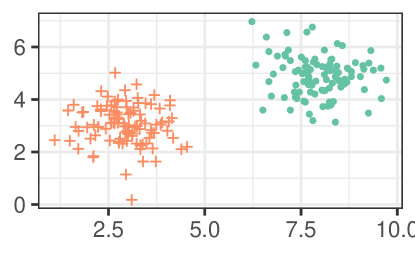
(b)

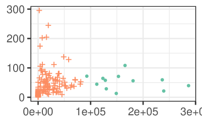
(c)

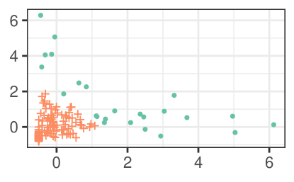
(d)

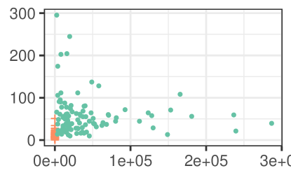
(e)

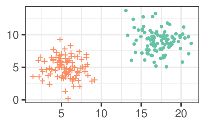
(f)

Figure 1: 1b shows the latent generated data. After transformation the observable data is shown in 1a. Two versions of $K$-means are shown in 1c and 1d. 1e shows the TiK-means results and 1f shows the inverse transformation of the data in 1a estimated by TiK-means.

$\bm{\lambda}=\{1.4,0.9\}$. The $K$-means algorithm with known $K$ does poorly (Figure 1c), with an ARI of just $0.013$. Clearly, the horizontal axis dominates the WSS because of its larger scale, so that $K$-means is pretty much only influenced by this coordinate in the clustering. Scaling the coordinates and then applying $K$-means visually improves performance (Figure 1d) but still has a low ARI of 0.055. The scaling helps $K$-means use both dimensions, but is not enough to isolate the small-valued cluster. The original clustering is however, perfectly (Figure 1e) recovered by our algorithm upon using both homogeneous and non-homogeneous transformations. Therefore, allowing $K$-means to transform the dataset as it assigned clusters helped TiK-means find and isolate the distinct but skewed groups: Figure 1f displays the homogeneous TiK-means solution in terms of the back-transformed dataset and shows perfectly separated and homogeneous spherically-dispersed clusters.

TABLE I: Performance, in terms of ARI of $K$-means, MBC and TiK-means on datasets for known and estimated $K$.

		Known K					Estimated K
					TiK-means						TiK-means
		K	K-means	MBC	$\lambda_{p}$	$\lambda_{k\times p}$	K-means		MBC		$\lambda_{p}$		$\lambda_{k\times p}$
	Unscaled		0.371	0.967	0.854	0.868	7	0.226	3	0.967	3	0.854	3	0.868
Wine	Scaled	3	0.898	0.930	0.854	0.933	7	0.528	3	0.930	3	0.854	3	0.933
	Unscaled		0.318	0.535	0.809	0.841	10	0.212	10	0.314	9	0.528	9	0.570
	Scaled	3	0.448	0.535	0.815	0.814	11	0.317	11	0.285	5	0.621	5	0.618
	Unscaled		0.444	0.649	0.761	0.781	10	0.424	10	0.591	9	0.761	9	0.781
Olive Oils	Scaled	9	0.632	0.659	0.629	0.622	11	0.542	11	0.544	5	0.780	5	0.778
	Unscaled		0.034	0.393	0.946	0.997	5	0.118	5	0.338	5	0.927	3	0.958
SDSS	Scaled	2	0.994	0.391	1	0.997	5	0.840	5	0.338	5	0.925	4	0.6709
	Unscaled		0.717	0.737	0.675	0.721	7	0.448	4	0.481	3	0.675	3	0.721
Seeds	Scaled	3	0.773	0.712	0.675	0.785	7	0.428	4	0.580	7	0.378	6	0.449
	Unscaled		0.532	0.640	0.570	-	20	0.524	19	0.557	13	0.639	-
Pen Digits	Scaled	10	0.524	0.633	0.556	-	20	0.562	20	0.480	8	0.546	-

III-B Performance on Classification Datasets

Our evaluations are on classification datasets with different $(n,p,K)$ that are popular for evaluating clustering algorithms. Our datasets have $n$ ranging from $n=150$ to $n=10992$ and $p$ from $p=3$ to $p=16$. We set $K_{\max}=\min(2K_{\mbox{true}}+1,20)$ when the $K$ needs to be estimated. In all cases, we evaluated performance on both scaled and unscaled datasets.

III-B1 Wines

This dataset [61, 62] has measurements on $p=13$ chemical components of 178 wines from $K=3$ (Barolo, Grignolino and Barbera) cultivars. TiK-means correctly estimates $K$ (see Figure 2 for the

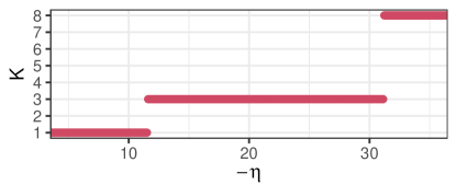
Figure 2: The Jump selection plot for the wines dataset. $\hat{K}=3$ is chosen, as every $\eta$ between the $\eta$s that choose $K=1$ and the $\eta$s that choose $K=8$ has a maximum jump statistic at $3$.

jump selection plot) with very good performance (Table I) that (in the non-homogeneous case) almost matches MBC which is known to perform well on this dataset. However, the much-abused $K$-means algorithm, while reasonably competitive for $K=3$ on the scaled dataset, chooses 8 groups for both the raw and scaled versions of the dataset when $K$ is not known. Performance is substantially poorer for such a high choice of $K$. However, TiK-means performs creditably and nearly recovers the MBC grouping.

III-B2 Olive Oils

The olive oils dataset [63, 64] contains the concentration of 8 different fatty acids in olive oils produced in 9 regions in 3 areas (North, South and Sardinia) of Italy. Clustering algorithms can be evaluated at a finer level (corresponding to regions) or a macro areal level. Observations are on similar scales so scaling is not recommended. However, we evaluate performance both with scaling and without scaling. With known $K=3$, TiK-Means recovers the true clusters better than $K$-means or MBC on both the scaled and unscaled dastasets, while for known $K=9$, TiK-means is the best performer (Table I) on the unscaled dataset. All algorithms perform similarly on the scaled dataset with $K=9$ groups. Non-homogeneous TiK-means betters its homogeneous cousin on the scaled dataset but is similar on the unscaled dataset.

With $K$ unknown, $K$-means and MBC both choose $K=10$ and 11 for the unscaled and scaled data. Without scaling, TiK-means chooses $K=9$, which matches the true number of regions, but with scaling, TiK-means chooses $K=5$. In either case, TiK-means betters the other algorithms for both unscaled and scaled datasets (Table I).

III-B3 Sloan Digital Sky Survey

The Sloan Digital Sky Survey (SDSS) documents physical measurements on hundreds of millions of astronomical objects. The small subset of data made available by [65] contains 1465 complete records quantifying brightness, size, texture, and two versions of shape (so $p=5$). Our objective is to differentiate galaxies from stars. Before applying TiK-means the dataset is slightly shifted in the texture and shape features so that each coordinate is positive. We do so to address the issue that the IHS transformation does not have a shift parameter and naturally splits dimensions at 0 irrespective of whether the split is coherent or not for clustering.

Table I indicates that $K$ is difficult to identify for all of the algorithms - none can correctly estimate it. Without scaling, the nonhomogeneous TiK-means algorithm chooses $K=3$ and gets the highest ARI of $0.958$ followed by the homogeneous algorithm with $K=5$ and an ARI of $0.927$. On the scaled dataset, the standard $K$-means jump statistic chooses $K=7$ and gets an ARI of $0.830$. When $K$ is known and fixed to be $2$ the results are more palatable. MBC unsurprisingly struggles, with the lowest ARIs except for the unscaled $K$-means algorithm. On the unscaled dataset, non-homogeneous TiK-means almost recovered the true grouping, with homogeneous TiK-means close behind. With scaling, homogeneous TiK-means is perfect while non-homogeneous TiK-means and $K$-means performed well.

III-B4 Seeds

The seeds dataset [66] contains seven features to differentiate 3 different kinds of wheat kernels. On this dataset, each method performs similarly with respect to clustering accuracy for known $K$ (Table I). With unknown $K$, only TiK-means correctly estimates $K$ on the unscaled dataset and is the best performer, while MBC at $\hat{K}=4$ is close but performs substantially worse, and $K$-means does even worse. All methods perform indifferently on the scaled dataset.

III-B5 Pen Digits

The pen digits dataset [67] contains $p=16$ similar-scaled features extracted from each of $n=10992$ handwritten numerical digits. (Because $Kp$ is reasonably large for this dataset, we only report homogeneous TiK-means as simultaneous optimization the $Kp$ transformation parameters over such a large-dimensional parameter space was not successful.) For this dataset, and with known $K=10$, scaling does not impact performance of TiK-means, K-means or MBC. MBC is the best performer with an ARI of 0.64 (Table I) while TiK-means marginally betters K-means.

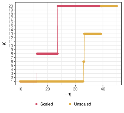
Figure 3: The jump selection plot for the scaled (red) and unscaled (gold) pen digits datasets.

For unknown $K$, Figure 3 indicates that for the scaled dataset, $K=8$ is the preference for every value of the exponent that chooses a $K$ between $K=1$ or $K=20$. For the unscaled dataset, $K=13$ is estimated for all but a couple $-\eta$ values. MBC chooses $K=19$ for the unscaled dataset but is indeterminate for the scaled version, returning the maximum $K=20$. $K$-means with the jump statistic [29] also can not estimate $K$ for both the scaled and unscaled datasets. In terms of performance, TiK-means at $K=8$ is marginally beaten by $K$-means at $K=20$ for the scaled dataset but is better than MBC. On the unscaled dataset, TiK-means is the indisputable best performer, almost recovering in ARI the performance of MBC with known $K=10$.

TABLE II: Confusion matrix of the true (rows), and the groups (columns) estimated by TiK-means for (a) $\hat{K}=8$ and (b) $\hat{K}=13$ for the scaled and unscaled datasets. The column names denote the author-specified digits that can be used to best characterize the TiK-means solutions.

      

	{0}	{1}	{2}	{3,9}	{4}	{5,8}	{6}	{7,8}
0	1032	3	10	0	11	0	85	2
1	0	664	355	120	2	0	2	0
2	0	19	1121	0	0	0	0	4
3	0	33	1	1020	1	0	0	0
4	0	9	1	6	1118	0	10	0
5	0	1	0	427	0	626	0	1
6	0	0	40	3	1	1	1011	0
7	0	145	25	8	0	4	56	904
8	215	10	44	26	0	323	34	403
9	17	243	0	672	122	0	0	1

(a) Scaled Dataset, $\hat{K}=8$

	{0}	{1}	{2}	{3}	{4}	{5}	{6}	{7}	{8}	{9}	{0}	{5,9}	{8}
0	550	0	5	0	6	0	21	0	1	2	537	0	21
1	0	645	279	69	1	0	12	54	0	63	0	20	0
2	0	15	1052	0	0	0	0	77	0	0	0	0	0
3	0	23	1	1024	1	0	0	0	0	2	0	4	0
4	1	14	4	0	1045	0	51	0	0	26	0	3	0
5	0	0	0	20	0	624	22	0	0	155	0	231	3
6	0	0	1	0	3	1	1048	0	0	0	3	0	0
7	0	149	19	74	1	4	1	891	2	0	0	0	1
8	9	0	9	44	0	5	2	18	453	5	6	71	433
9	14	32	0	25	91	0	0	0	0	626	0	266	1

(b) Unscaled Dataset, $\hat{K}=13$

Table IIa shows the confusion matrix for the TiK-means clustering with $8$ groups on the scaled dataset. The column names show the digit truths that the TiK-means clusters seem to recover. The diagonal elements of the table show that digits are grouped correctly together, with $0$s, $1$s, $2$s, $3$s, $4$s, $6$s, $7$s, and $9$s grouped well, even though $3$s and $9$s are grouped together. Many $5$s and $8$s share a cluster, but other $5$s tend to be grouped with $3$s and $9$s, while other $8$s are usually grouped with $7$s. For true $K=10$, the confusion matrix (Table S-9) indicates not much benefit in pre-specifying $K=10$. Though the additional clusters available to TiK-means succeeds in separating the {7,8} group, $0$s are also split into two different groups with the other extra cluster rather than resolving the mistakes made with clustering $5$s. On the unscaled dataset (Table IIb), and with $K=13$, every digit has a cluster mostly to itself. The three additional groups split the $0$s into another cluster, one splits the 8s into a new cluster, and one contains a mixture of $5$s and $9$s. Expectedly, the common defined clusters for both the scaled and unscaled TiK-means results match almost perfectly. The better performance with $K=13$ indicates a commonly-observed trait in handwriting classification, that is, that there is substantial variation in writing digits with more curves or edges.

The results of our experiments show the success of TiK-means in overcoming the homogeneous-dispersions assumption of $K$-means while remaining within the scope of the algorithm. It performs competitively with regards to clustering accuracy on all of the datasets presented, sometimes performing much better than $K$-means and MBC. TiK-means is generally as good or better at recovering the true number of clusters as MBC, and is much better than the jump statistic with the default transformation power. TiK-means estimates $K$ more closely when the data is not scaled beforehand, reinforcing our earlier suggestion to eschew scaling unless necessitated for the $\bm{\lambda}$ search. We now use it to analyze the GRB dataset.

IV Application to Gamma Ray Bursts dataset

As discussed in Section I-A, GRB datasets have so far primarily been analyzed on the $\log_{10}$ scale to remove skewness before clustering. This summary transformation reduces skewness in the marginals but is somewhat arbitrary with no regard for any potential effects on analysis. TiK-means allows us to obtain data-driven transfomations of the variables while clustering. In this application, the features have vastly different scales, so we have scaled the data on the lines of the discussion in Section II-C2 to more readily specify the $\bm{\Lambda}$ grid for estimating the IHS transformation parameters.

Figure 4 displays the

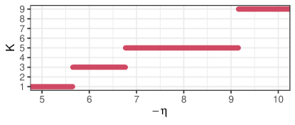
Figure 4: The jump selection plot for the GRB dataset that shows support for 3 groups but more support for $\hat{K}=5$.

[autoplay,loop,width=0.25]1Plots/radviz3d_grb13

(a)

GRB Cluster Summaries k Size T₉₀ Fluence Hardness₃₂₁ Duration/Fluence/Spectrum 1 330 -0.278$\pm$0.55 -29.682$\pm$1.20 0.446$\pm$0.02 short/faint/soft 2 448 1.709$\pm$0.39 -22.988$\pm$1.13 0.460$\pm$0.02 long/bright/hard 3 190 1.496$\pm$0.49 -20.576$\pm$1.61 0.443$\pm$0.02 long/bright/soft 4 197 0.241$\pm$0.58 -26.397$\pm$1.13 0.448$\pm$0.02 intermediate/intermediate/soft 5 435 1.408$\pm$0.39 -25.779$\pm$1.61 0.468$\pm$0.02 long/intermediate/hard

(b)

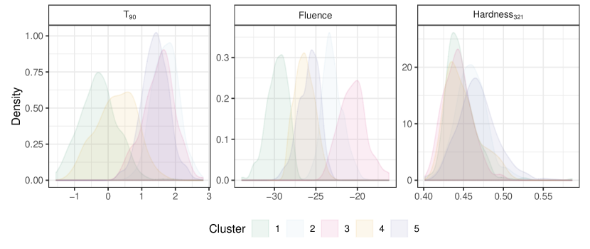
(c)

Figure 5: TiK-means clustering of the GRB dataset. (a) Three-dimensional radial visualization plot [68] of obtained groups in transformed space. (b, c) Summary of duration ($T_{90}$), total fluence $F_{total}$, and spectral hardness $H_{321}$, introduced in [47], for each of the five groups obtained using TiK-means.

jump selection plot for $K$. For $\eta\in(-4.31,-4.83)$, we are recommended a 3-groups solution, but a much larger interval for $\eta\in(-4.83,-6.27)$, recommends 5 kinds of GRBs in the BATSE 4Br database. So the jump selection plot suggests some support for the 3-groups TiK-means solution but has a clear and overwhelming preference for the partitioning with $K=5$. (A similar observation holds for TiK-means on the unscaled dataset.) Thus, even with $K$-means, but done on objectively-chosen transformed spaces, our results demonstrate support for the presence of five distinct types of GRBs [49] than the previously disputed two-or-three types of GRBs which summarily used log-transformed variables and used $K$-means and the Jump statistic [51], but which upon careful examination [48] was actually indeterminate. Our five groups are distinct, as per the three-dimensional radial visualization [68] plot in Figure 5a which displays the most-separated projections of the transformed dataset. We now discuss the characteristics of the obtained groups in terms of three summary characterizations commonly used in the astrostatistics literature [47] to describe the physical properties of GRBs. These characterizations are the duration $(T_{90})$, total fluence $(F_{total}=F_{1}+F_{2}+F_{3}+F_{4})$, and spectral hardness $H_{321}={F_{3}}/({F_{1}+F_{2}})$.

Figure 5 summarizes performance in terms of these three summary statistics. We use the traditional $\log_{10}$ scale for these summaries in describing our groups in order to preserve their physical interpretations. The burst duration variable $T_{90}$ shows three groups clumped in the long duration range, and an intermediate and a short duration cluster that has some separation from the large group. The total fluence variable shows 5 homogeneous and approximately equally-spaced groups with fairly good separation between each other. The spectral hardness shows less separation than the other values, but has a soft group and a hard group that are partially separated. The three summary statistics characterize our groups in terms of the paradigm of duration/fluence/spectrum as follows: (1) long/intermediate/hard, (2) intermediate/intermediate/soft, (3) short/faint/soft, (4) long/bright/hard, and (5) long/bright/soft. The fourth and fifth groups have high fluence, but the latter is brighter and could belong to its own very bright fluence class.

We end our discussion here by noting that Figure 5c also provides an indication of the reason behind the controversy between 2 and 3 GRB groups in the astrophysics community. When restricting attention only to the most commonly used duration variables, it is easy to see why there would be differing interpretation between 2 or 3 groups. However, incorporating the additional information separates out Groups 2, 4 and 5, as can be seen from the plots of total fluence and spectral hardness. Our TiK-means solution presents groups that are distinct, interpretable and in line with newer results obtained using carefully done Gaussian [48] or $t$-mixtures [49] model-based or nonparametric syncytial [50] clustering.

V Conclusions

In this paper, we present a modification of $K$-means called the TiK-means algorithm that preserves the simplicity and computational advantages of $K$-means while recovering groups of varying complexities. The efficient and ubiquitous $K$-means clustering algorithm has inherent underlying distributional assumptions of homogeneous spherically dispersed groups. Such assumptions are crucial to its good performance and several alternatives exist, but practitioners routinely use it without regard to its applicability in the given context. These assumptions are relaxed in the TiK-means framework, allowing for more robust application of the $K$-means algorithm.

We provide a modified Jump statistic [29] to determine the number of groups. The jump statistic is dependent on a parameter ($\eta$) that represents the number of effective dimensions in the dataset [29] and can greatly impact performance. We desensitize our method to the choice of $\eta$ by calculating our modified jump-selected $\hat{K}$ for a range of $\eta$s in a display called the jump selection plot and choosing the one that is supported by the largest range of $\eta$s. Our algorithm is made available to the scientific community through a publicly available R [69] package at https://github.com/berryni/TiKmeans and performs creditably on several examples where the groups are not homogeneous and spherically dispersed. Finally, we weigh in on the distinct kinds of GRBs in the BATSE 4Br catalog. Most astrophysicists have hitherto used $K$-means on a few features to arrive at two or three groups in findings that had split the community between two camps, one advocating for either solution. Recent work [48, 49] showed that the $K$-means solutions were neither tenable nor determinate in terms of finding the kinds of GRBs and that in reality, MBC with the Bayesian Information Criterion indicates five groups of clusters. Our analysis of the GRB dataset using TiK-means confirms this finding and shows five well-separated groups, shedding more light into this long-standing question with implications on the origin of the universe.

There are a number of areas that could benefit from further work. One potential downside to our algorithm when compared to $K$-means is the running time which can quickly increase with $p$ and/or the fineness of the search grid for $\bm{\lambda}$. We also need to have a better understanding of the convergence properties of the algorithm. While the convergence of the algorithm has not been proven like in the case of traditional $K$-means, for any reasonable number of starting points the algorithm converges to consistent values of both $\bm{\lambda}$ and cluster assignments. However, it is conceivable that there exist cases where $\bm{\lambda}$ and the cluster assignments reach a point where they never converge, and instead oscillate back and forth. We know that $K$-means alone will converge to a local minimum and that a hill climbing $\bm{\lambda}$ step will as well, but it would be worth investigating if both happening simultaneously guarantees local convergence. Additionally, the current algorithm is implemented in conjunction with a Lloyd’s algorithm [22]. While easy to follow and modify, later algorithms do a better job at reducing the number of computations and limiting compute time. Attempting a Hartigan-Wong-style algorithm [23] could speed up TiK-means. Here, care should be taken with regards to the live set because as $\bm{\lambda}$ changes from iteration to iteration, some of the assumptions made to allow for the shortcuts in the Hartigan-Wong algorithm may no longer be immediate and may need rework. Increasing $n$ has a smaller impact on running time than increasing $p$ because the expensive optimization step is over the $\bm{\lambda}$ space and relates to $p$. Finally, the TiK-means algorithm has been developed and illustrated in the context of the IHS transformation. While the performance of TiK-means using the IHS is quite good, additional flexibility provided by, for instance, the Yeo-Johnson and the two-parameter Box-Cox transformations may further improve performance. Our development is general enough to allow for such transformations, but it would be worth evaluating their performance. Thus, we see that notwithstanding our comprehensive approach to finding skewed and heterogeneous-dispersed groups within the context of $K$-means, issues meriting further attention remain.

Supplementary Materials

S-6 Supplementary Materials

We include information about TiK-means clustering results that were not included in the paper.

S-6.1 Wines

Confusion matrices for the Wine dataset TiK-means results are shown in Tables S-3.

TABLE S-3: (a) TiK-means results for the scaled and unscaled wines dataset (results are identical) with a $p$-dimensional $\bm{\lambda}$. TiK-means results iwth the $k\times p$-dimensional $\bm{\lambda}$ for the (b) scaled and (c) unscaled datasets.

Unscaled/Scaled ($\bm{\lambda}_{p}$)
	TiK-means
1	59	0	0
2	2	62	7
3	0	0	48

(a)

Unscaled ($\bm{\lambda}_{k\times p}$)
	TiK-means
1	59	0	0
2	2	63	6
3	0	0	48

(b)

Scaled ($\bm{\lambda}_{k\times p}$)
	TiK-means
1	59	0	0
2	1	67	3
3	0	0	48

(c)

S-6.2 Iris

S-6.21 Iris

The celebrated Iris dataset [70, 71] has lengths and widths of petals and sepals on 50 observations each from three Iris’ species: I. setosa, I. virginica and I. versicolor. The first species is very different from the others that are less differentiated in terms of sepal and petal lengths and widths. At the true $K$, MBC has the highest ARI at $0.904$, with 5 misclassifications. Non-homogeneous TiK-means is close, with 6 misclassifications and an ARI of $0.886$. Homogeneous TiK-means has 8 misclassifications and an ARI of $0.851$. $K$-means performs poorly on both the scaled and unscaled data, although if the Iris dataset is scaled and not centered a priori, then it matches the performance of non-homogeneous TiK-means. Despite this improvement, there is little reason to scale the dataset before $K$-means without knowing the true cluster assignments in advance. Only nonhomogeneous TiK-means on the scaled dataset recovers the true number of clusters, while MBC and homogeneous TiK-means both choose $K=2$. $K$-means fails to choose $K$ with the default $\eta=2$, although using the jump statistic with $\eta=4$ chooses $K=3$ [29].

Despite the $p$ - dimensional version of TiK-means missing two data points more than the best version of the base $K$-means algorithm, TiK-means was run on the dataset without manipulation whereas base $K$-means only performed well on the dataset that was scaled by Root Mean Square $\left(\text{RMS}({\bm{x}})=\sqrt{\frac{1}{n-1}\sum_{i=1}^{n}x_{i}^{2}}\right)$ without centering. While manipulating a dataset before clustering is generally fine it is difficult to know exactly which way it should be scaled in the case that the true clusters are unknown, and there is little reason to scale the iris dataset by RMS unless the true cluster assignments are known.

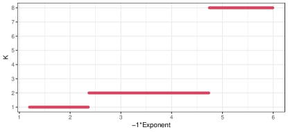
(a)

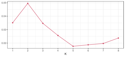
(b)

Figure S-1: The selection of $K$ using the jump statistic on the iris dataset: (a) Plot of Jump statistic $K$ against $\eta$ and (b) Jump Statistic slice at $\eta=-3$. $K=2$ is the value chosen.

Because the labels of the iris dataset are known, it is common to cluster the dataset with 3 clusters. Without the labels it is less obvious how many clusters should be used, although 2 or 3 are the obvious answers. Using the algorithm for number of cluster selection outlined in Section II-C3, our method chooses 2 clusters as the best way to cluster the data. In Figure S-1a, as you follow the dots from left to right, the selection of number of clusters goes from 1 to 2, and then to 8.

At $\eta=-3$ the method chooses $k=2$. The plot in Figure S-1b shows the jump statistics from the transformed objective functions that were chosen between. In this case $k=2$ had the largest value, followed by $k=3$. This decision between $k=2$ and $k=3$ matches our intuition for the problem.

Tables S-4a and S-4b show the confusion matrices from the TiK-means clustering results for $K=3$ and $p$ and $k\times p$-dimensional $\bm{\lambda}$s, respectively.

TABLE S-4: Confusion matrix for Iris dataset when clustered using TiK-means with (a) $p$-dimensional $\bm{\lambda}$ and (b) $k\times p$-dimensional $\bm{\lambda}$.

           

Iris Dataset ($\bm{\lambda}_{p}$)
	TiK-means
Setosa	50	0	0
Versicolor	0	46	4
Virginica	0	4	46

(a)

Iris Dataset ($\bm{\lambda}_{k\times p}$)
	TiK-means
Setosa	50	0	0
Versicolor	0	48	2
Virginica	0	4	46

(b)

S-6.3 Olive Oils

S-6.31 Macro Regions $(K=3)$

Tables S-5 show the confusion matrices from the TiK-means clustering results for $K=3$ and $p$ and $k\times p$-dimensional $\bm{\lambda}$s, respectively for the scaled and unscaled datasets.

TABLE S-5: Confusion matrix for the Olive Oils dataset when clustered using TiK-means with $K=3$ and (a) $p$-dimensional $\bm{\lambda}$ (b) $k\times p$-dimensional $\bm{\lambda}$, for the scaled dataset. Corresponding results for the scaled dataset are in (c) and (d). (e) Results obtained on the scaled (and unscaled) dataset for $\hat{K}=5$ groups.

                   

Olive Oils Dataset - Unscaled ($k=3$, $\bm{\lambda}_{p}$)
	TiK-means
South	323	0	0
Sardinia	0	98	0
Centre.North	0	114	37

(a)

Olive Oils Dataset - Unscaled ($k=3$, $\bm{\lambda}_{p\times k}$)
	TiK-means
South	322	1	0
Sardinia	0	98	0
Centre.North	0	67	84

(b)

Olive Oils Dataset - Scaled ($k=3$, $\bm{\lambda}_{p}$)
	TiK-means
South	323	0	0
Sardinia	0	98	0
Centre.North	0	98	53

(c)

Olive Oils Dataset - Scaled ($k=3$, $\bm{\lambda}_{p\times k}$)
	TiK-means
South	323	0	0
Sardinia	0	98	0
Centre.North	0	100	51

(d)

Olive Oils Dataset - Scaled ($k=5$, $\bm{\lambda}_{p}$)
	TiK-means
South	218	0	0	105	0
Sardinia	0	98	0	0	0
Centre.North	0	2	99	0	50

(e)

S-6.32 Micro Regions $(K=9)$

Tables S-6 show the confusion matrices from the TiK-means clustering results for $K=9$ and $p$ and $k\times p$-dimensional $\bm{\lambda}$s, respectively.

TABLE S-6: Confusion matrix for the Olive Oils dataset when clustered using TiK-means with $K=9$ and (a) $o$-dimensional $\bm{\lambda}$ and (b) $k\times p$-dimensional $\bm{\lambda}$. for the unscaled and (c, d) scaled datasets.

               

Olive Oils Dataset - Unscaled ($k=9$, $\bm{\lambda}_{p}$)
	TiK-means
Apulia.north	23	2	0	0	0	0	0	0	0
Calabria	0	56	0	0	0	0	0	0	0
Apulia.south	0	13	193	0	0	0	0	0	0
Sicily	14	15	7	0	0	0	0	0	0
Sardinia.inland	0	0	0	0	65	0	0	0	0
Sardinia.coast	0	0	0	0	33	0	0	0	0
Liguria.east	0	0	0	0	0	3	11	0	36
Liguria.west	0	0	0	7	0	8	16	19	0
Umbria	0	0	0	0	0	0	0	0	51

(a)

Olive Oils Dataset - Unscaled ($k=9$, $\bm{\lambda}_{p\times k}$)
	TiK-means
Apulia.north	23	2	0	0	0	0	0	0	0
Calabria	0	56	0	0	0	0	0	0	0
Apulia.south	0	15	191	0	0	0	0	0	0
Sicily	14	15	7	0	0	0	0	0	0
Sardinia.inland	0	0	0	0	65	0	0	0	0
Sardinia.coast	0	0	0	0	33	0	0	0	0
Liguria.east	0	0	0	0	0	11	34	3	2
Liguria.west	0	0	0	7	0	16	0	27	0
Umbria	0	0	0	0	0	0	0	0	51

(b)

Olive Oils Dataset - Scaled ($k=9$, $\bm{\lambda}_{p}$)
	TiK-means
Apulia.north	23	2	0	0	0	0	0	0	0
Calabria	0	54	2	0	0	0	0	0	0
Apulia.south	0	7	139	60	0	0	0	0	0
Sicily	14	15	6	1	0	0	0	0	0
Sardinia.inland	0	0	0	0	65	0	0	0	0
Sardinia.coast	0	0	0	0	33	0	0	0	0
Liguria.east	0	0	0	0	0	0	43	3	4
Liguria.west	0	0	0	0	0	21	2	27	0
Umbria	0	0	0	0	0	0	0	0	51

(c)

Olive Oils Dataset - Scaled ($k=9$, $\bm{\lambda}_{k\times p}$)
	TiK-means
Apulia.north	24	1	0	0	0	0	0	0	0
Calabria	1	54	1	0	0	0	0	0	0
Apulia.south	0	6	137	63	0	0	0	0	0
Sicily	17	14	3	2	0	0	0	0	0
Sardinia.inland	0	0	0	0	64	0	0	0	1
Sardinia.coast	0	0	0	0	33	0	0	0	0
Liguria.east	0	0	0	0	0	6	37	3	4
Liguria.west	0	0	0	0	0	23	0	27	0
Umbria	0	0	0	0	0	0	4	0	47

(d)

S-6.4 Seeds

Confusion matrices for the Seeds dataset using TiK-means vis-a-vis the true grouping are in Table S-7.

TABLE S-7: Confusion matrices for Seeds dataset when clustered with TiK-means at (a-c) true and (d) estimated $K$.

                                   

Seeds - Scaled/Unscaled ($K=3$, $\bm{\lambda}_{p}$)
	TiK-means
Kama	55	2	13
Rosa	9	61	0
Canadian	2	0	68

(a)

Seeds - Scaled ($K=3$, $\bm{\lambda}_{k\times p}$)
	TiK-means
Kama	63	1	6
Rosa	5	65	0
Canadian	4	0	66

(b)

Seeds - Unscaled ($K=3$, $\bm{\lambda}_{k\times p}$)
	TiK-means
Kama	58	1	11
Rosa	10	60	0
Canadian	0	0	70

(c)

Seeds - Scaled ($\hat{K}=7$, $\bm{\lambda}_{p}$)
	TiK-means
Kama	27	0	2	4	0	12	25
Rosa	0	30	0	17	21	0	2
Canadian	3	0	39	0	0	28	0

(d)

Seeds - Scaled ($\hat{K}=6$, $\bm{\lambda}_{k\times p}$)
	TiK-means
Kama	35	0	4	13	16	2
Rosa	0	44	0	0	10	16
Canadian	0	0	50	20	0	0

(e)

S-6.5 SDSS

Confusion matrices for the SDSS dataset using TiK-means vis-a-vis the true grouping are in Table S-8.

TABLE S-8: Confusion matrices for the SDSS dataset when clustered with TiK-means with true K=2 and estimated $\hat{K}$.

                       

SDSS - Unscaled ($k=2$, $\bm{\lambda}_{p}$)
	TiK-means
	0	1178
	270	17

(a)

SDSS - Unscaled ($K=2$, $\bm{\lambda}_{k\times p}$)
	TiK-means
	1	1177
	287	0

(b)

SDSS - Scaled ($K=2$, $\bm{\lambda}_{p}$)
	TiK-means
	0	1178
	287	0

(c)

SDSS - Scaled ($K=2$, $\bm{\lambda}_{k\times p}$)
	TiK-means
	1	1177
	287	0

(d)

SDSS - Scaled ($\hat{K}=5$, $\bm{\lambda}_{p}$)
	TiK-means
	1	2	1164	11	0
	0	0	0	201	86

(e)

SDSS - Unscaled ($\hat{K}=5$, $\bm{\lambda}_{p}$)
	TiK-means
	3	2	0	1165	1
	6	0	86	0	0

(f)

SDSS - Scaled ($\hat{K}=4$, $\bm{\lambda}_{k\times p}$)
	TiK-means
	31	0	1139	8
	0	96	10	181

(g)

SDSS - Unscaled ($\hat{K}=3$, $\bm{\lambda}_{k\times p}$)
	TiK-means
	17	1161	0
	0	0	287

(h)

S-6.6 Pen Digits

Table S-9 shows the confusion matrix of the TiK-means solution at the true $K=10$.

TABLE S-9: Confusion matrix for the (a) scaled and (b) unscaled datasets showing differences between the true clusters, indicated by rows, and the TiK-means estimated clusters for $K=10$, indicated by rows. The column names denote the author specified digits that the TiK-means clusters seem to cover.

Pen Digits - Scaled
	TiK-means
	{0i}	{1}	{2}	{3,5,9}	{4}	{5,8}	{6}	{7}	{8}	{0ii}
0	553	3	4	0	11	0	1	6	46	519
1	0	660	344	136	2	0	1	0	0	0
2	0	22	1118	0	0	0	0	4	0	0
3	0	40	1	1014	0	0	0	0	0	0
4	0	9	1	5	1117	0	12	0	0	0
5	0	1	0	427	0	624	0	0	3	0
6	0	0	24	3	1	1	1027	0	0	0
7	0	142	8	4	1	2	18	960	7	0
8	27	10	22	22	0	332	6	97	410	129
9	0	190	0	662	179	0	0	0	1	23

(a)

Pen Digits - Unscaled - K = 10
	TiK-means
	{0i}	{1}	{2}	{3,9}	{4}	{5}	{6}	{7,8}	{0,8}	{5,9}
0	693	3	14	0	6	0	17	0	410	0
1	0	652	322	57	1	0	3	14	0	94
2	0	15	1128	1	0	0	0	0	0	0
3	0	24	1	1012	2	0	0	0	0	16
4	0	34	8	13	1046	0	23	0	0	20
5	0	0	0	94	0	627	1	0	0	333
6	0	0	5	0	1	1	1044	0	0	5
7	0	156	9	30	0	4	49	894	0	0
8	18	1	18	12	0	126	45	345	432	58
9	16	70	0	598	98	0	0	1	0	272

(b)

References

- [1] F. Murtagh, Multi-Dimensional Clustering Algorithms. Berlin; New York: Springer-Verlag, 1985.
- [2] D. B. Ramey, “Nonparametric clustering techniques,” in Encyclopedia of Statistical Science. New York: Wiley, 1985, vol. 6, pp. 318–319.
- [3] G. J. McLachlan and K. E. Basford, Mixture Models: Inference and Applications to Clustering. New York: Marcel Dekker, 1988.
- [4] L. Kaufman and P. J. Rousseuw, Finding Groups in Data. New York: John Wiley & Sons, 1990.
- [5] B. S. Everitt, S. Landau, and M. Leesem, Cluster Analysis (4th Ed.). New York: Hodder Arnold, 2001.
- [6] C. Fraley and A. E. Raftery, “Model-Based Clustering, Discriminant Analysis, and Density Estimation,” Journal of the American Statistical Association, vol. 97, pp. 611–631, 2002.
- [7] R. J. Tibshirani and G. Walther, “Cluster validation by prediction strength,” Journal of Computational and Graphical Statistics, vol. 14, no. 3, pp. 511–528, 2005.
- [8] J. R. Kettenring, “The practice of cluster analysis,” Journal of classification, vol. 23, pp. 3–30, 2006.
- [9] R. Xu and D. C. Wunsch, Clustering. NJ, Hoboken: John Wiley & Sons, 2009.
- [10] C. D. Michener and R. R. Sokal, “A quantitative approach to a problem in classification,” Evolution, vol. 11, pp. 130–162, 1957.
- [11] A. Hinneburg and D. Keim, “Cluster discovery methods for large databases: From the past to the future,” in Proceedings of the ACM SIGMOD International Conference on the Management of Data, 1999.
- [12] M. E. Celebi, H. A. Kingravi, and P. A. Vela, “A comparative study of efficient initialization methods for the k-means clustering algorithm,” Expert Systems with Applications, vol. 40, no. 1, pp. 200–210, 2013.
- [13] R. Maitra, V. Melnykov, and S. Lahiri, “Bootstrapping for significance of compact clusters in multi-dimensional datasets,” Journal of the American Statistical Association, vol. 107, no. 497, pp. 378–392, 2012.
- [14] R. Maitra, “Clustering massive datasets with applications to software metrics and tomography,” Technometrics, vol. 43, no. 3, pp. 336–346, 2001.
- [15] S. Johnson, “Hierarchical clustering schemes,” Psychometrika, vol. 32:3, pp. 241–254, 1967.
- [16] A. Jain and R. Dubes, Algorithms for Clustering Data. Englewood Cliffs, NJ: Prentice Hall, 1988.
- [17] E. Forgy, “Cluster Analysis of Multivariate Data: Efficiency vs. Interpretability of Classifications,” Biometrics, vol. 21, pp. 768–780, 1965.
- [18] J. MacQueen, “Some methods for classification and analysis of multivariate observations,” in Proceedings of the Fifth Berkeley Symposium on Mathematical Statistics and Probability, Volume 1: Statistics. Berkeley, Calif.: University of California Press, 1967, pp. 281–297.
- [19] D. Titterington, A. Smith, and U. Makov, Statistical Analysis of Finite Mixture Distributions. Chichester, U.K.: John Wiley & Sons, 1985.
- [20] G. McLachlan and D. Peel, Finite Mixture Models. New York: John Wiley and Sons, Inc., 2000.
- [21] V. Melnykov and R. Maitra, “Finite mixture models and model-based clustering,” Statistics Surveys, vol. 4, pp. 80–116, 2010.
- [22] S. Lloyd, “Least Squares Quantization in PCM,” IEEE Transactions on Information Theory, vol. 28, no. 2, pp. 129–137, Mar. 1982.
- [23] J. A. Hartigan and M. A. Wong, “Algorithm AS 136: A K-Means Clustering Algorithm,” Journal of the Royal Statistical Society. Series C (Applied Statistics), vol. 28, no. 1, pp. 100–108, 1979.
- [24] R. Maitra, “Initializing Partition-Optimization Algorithms,” IEEE/ACM Transactions on Computational Biology and Bioinformatics, vol. 6, pp. 144–157, 2009.
- [25] W. J. Krzanowski and Y. Lai, “A criterion for determining the number of groups in a data set using sum-of-squares clustering,” Biometrics, vol. 44, no. 1, pp. 23–34, 1985.
- [26] G. W. Milligan and M. C. Cooper, “An examination of procedures for etermining the number of clusters in a dataset,” Psychometrika, vol. 50, pp. 159–179, 1985.
- [27] G. Hamerly and C. Elkan, “Learning the k in k-means,” in NIPS, vol. 3, 2003, pp. 281–288.
- [28] D. Pelleg and A. Moore, “X-means: Extending K-means with Efficient Estimation of the Number of Clusters,” in In Proceedings of the 17th International Conf. on Machine Learning. Morgan Kaufmann, 2000, pp. 727–734.
- [29] C. A. Sugar and G. M. James, “Finding the number of clusters in a dataset,” Journal of the American Statistical Association, vol. 98, no. 463, 2003.
- [30] J. T. Chi, E. C. Chi, and R. G. Baraniuk, “K-POD: A Method for k-Means Clustering of Missing Data,” The American Statistician, vol. 70, no. 1, pp. 91–99, 2016.
- [31] A. Lithio and R. Maitra, “An efficient k-means clustering algorithm for datasets with incomplete records,” Statistical Analysis and Data Mining – The ASA Data Science Journal, vol. 11, pp. 296–311, 2018.
- [32] L. Kaufman and P. J. Rousseeuw, “Clustering by means of Medoids,” in Statistical Data Analysis Based on the L1–Norm and Related Methods, Y. Dodge, Ed. North-Holland, 1987, pp. 405–416.
- [33] H. Park and C. Jun, “A simple and fast algorithm for K-medoids clustering,” Expert Systems with Applications, vol. 36, no. 2, pp. 3336–3341, 2009.
- [34] P. S. Bradley, O. L. Mangasarian, and W. N. Street, “Clustering via Concave Minimization,” in Advances in Neural Information Processing Systems, M. C. Mozer, M. I. Jordan, and T. Petsche, Eds., vol. 9. Cambridge, Massachusetts: MIT Press, 1997, pp. 368–374.
- [35] M. A. Carreira-Perpiñán and W. Wang, “The K-modes algorithm for clustering,” CoRR, vol. abs/1304.6478, 2013.
- [36] A. D. Chaturvedi, P. E. Green, and J. D. Carroll, “K-modes clustering,” Journal of Classification, vol. 18, pp. 35–56, 2001.
- [37] Z. Huang, “Clustering large data sets with mixed numeric and categorical values,” in Proceedings of the First Pacific Asia Knowledge Discovery and Data Mining Conference. Singapore: World Scientific, 1997, pp. 21–34.
- [38] E. P. Mazets, S. V. Golenetskii, V. N. Ilinskii, V. N. Panov, R. L. Aptekar, I. A. Gurian, M. P. Proskura, I. A. Sokolov, Z. I. Sokolova, and T. V. Kharitonova, “Catalog of cosmic gamma-ray bursts from the KONUS experiment data. I.” Astrophysics and Space Science, vol. 80, pp. 3–83, Nov. 1981.
- [39] J. P. Norris, T. L. Cline, U. D. Desai, and B. J. Teegarden, “Frequency of fast, narrow gamma-ray bursts,” Nature, vol. 308, p. 434, Mar. 1984.
- [40] J.-P. Dezalay, C. Barat, R. Talon, R. Syunyaev, O. Terekhov, and A. Kuznetsov, “Short cosmic events - A subset of classical GRBs?” in American Institute of Physics Conference Series, ser. American Institute of Physics Conference Series, W. S. Paciesas and G. J. Fishman, Eds., vol. 265, 1992, pp. 304–309.
- [41] C. Kouveliotou, C. A. Meegan, G. J. Fishman, N. P. Bhat, Michael S. Briggs, T. M. Koshut, W. S. Paciesas, and G. N. Pendleton, “Identification of two classes of gamma-ray bursts,” The Astrophysical Journal, vol. 413, pp. L101–L104, Aug. 1993.
- [42] I. Horvath, “A further study of the BATSE Gamma-Ray Burst duration distribution,” Astronomy & Astrophysics, vol. 392, no. 3, pp. 791–793, Sep. 2002.
- [43] D. Huja, A. Meszaros, and J. Ripa, “A comparison of the gamma-ray bursts detected by BATSE and Swift,” Astronomy & Astrophysics, vol. 504, no. 1, pp. 67–71, Sep. 2009.
- [44] M. Tarnopolski, “Analysis of Fermi gamma-ray burst duration distribution,” Astronomy & Astrophysics, vol. 581, p. A29, Sep. 2015.
- [45] I. Horvath and B. G. Toth, “The duration distribution of Swift Gamma-Ray Bursts,” Astrophysics and Space Science, vol. 361, no. 5, p. 155, Apr. 2016.
- [46] H. Zitouni, N. Guessoum, W. J. Azzam, and R. Mochkovitch, “Statistical study of observed and intrinsic durations among BATSE and Swift/BAT GRBs,” Astrophysics and Space Science, vol. 357, no. 1, p. 7, Apr. 2015.
- [47] S. Mukherjee, E. D. Feigelson, G. Jogesh Babu, F. Murtagh, C. Fraley, and A. Raftery, “Three Types of Gamma-Ray Bursts,” The Astrophysical Journal, vol. 508, no. 1, pp. 314–327, Nov. 1998.
- [48] S. Chattopadhyay and R. Maitra, “Gaussian-Mixture-Model-based Cluster Analysis Finds Five Kinds of Gamma Ray Bursts in the BATSE Catalog,” Monthly Notices of the Royal Astronomical Society, vol. 469, no. 3, pp. 3374–3389, Aug. 2017.
- [49] ——, “Multivariate $t$-Mixtures-Model-based Cluster Analysis of BATSE Catalog Establishes Importance of All Observed Parameters, Confirms Five Distinct Ellipsoidal Sub-populations of Gamma Ray Bursts,” Monthly Notices of the Royal Astronomical Society, Jul. 2018.
- [50] I. Almodóvar-Rivera and R. Maitra, “Kernel-estimated Nonparametric Overlap-Based Syncytial Clustering,” arXiv:1805.09505 [stat], May 2018.
- [51] T. Chattopadhyay, R. Misra, A. K. Chattopadhyay, and M. Naskar, “Statistical Evidence for Three Classes of Gamma-Ray Bursts,” Astrophysical Journal, vol. 667, no. 2, p. 1017, 2007.
- [52] G. E. P. Box and D. R. Cox, “An Analysis of Transformations,” Journal of the Royal Statistical Society. Series B (Methodological), vol. 26, no. 2, pp. 211–252, 1964.
- [53] B. F. J. Manly, “Exponential Data Transformations,” Journal of the Royal Statistical Society. Series D (The Statistician), vol. 25, pp. 37–42, 1976.
- [54] P. J. Bickel and K. A. Doksum, “An Analysis of Transformations Revisited,” Journal of the American Statistical Association, vol. 76, pp. 296–311, 1981.
- [55] I.-K. Yeo and R. A. Johnson, “A New Family of Power Transformations to Improve Normality or Symmetry,” Biometrika, vol. 87, no. 4, pp. 954–959, 2000.
- [56] J. B. Burbidge, L. Magee, and A. L. Robb, “Alternative Transformations to Handle Extreme Values of the Dependent Variable,” Journal of the American Statistical Association, vol. 83, no. 401, pp. 123–127, Mar. 1988.
- [57] P. Billingsley, Probability and Measure, ser. Wiley Series in Probability and Mathematical Statistics. Wiley, 1986.
- [58] R. Maitra and V. Melnykov, “Simulating data to study performance of finite mixture modeling and clustering algorithms,” Journal of Computational and Graphical Statistics, vol. 19, no. 2, pp. 354–376, 2010.
- [59] V. Melnykov and R. Maitra, “CARP: Software for Fishing Out Good Clustering Algorithms,” Journal of Machine Learning Research, vol. 12, pp. 69 – 73, 2011.
- [60] C. Fraley and A. E. Raftery, “MCLUST Version 3 for R: Normal Mixture Modeling and Model-Based Clustering,” University of Washington, Department of Statistics, Seattle, WA, Tech. Rep. 504, 2006.
- [61] M. Forina, R. Leardi, and S. Lanteri, “PARVUS - An Extendible Package for Data Exploration, Classification and Correlation,” 1988.
- [62] D. C. S. Aeberhard and O. de Vel, “Comparison of Classifiers in High Dimensional Settings,” Department of Computer Science and Department of Mathematics and Statistics, James Cook University of North Queensland, Tech. Rep. 92-02, 1992.
- [63] M. Forina and E. Tiscornia, “Pattern recognition methods in the prediction of Italian olive oil origin by their fatty acid content,” Annali di Chimica, vol. 72, pp. 143–155, 1982.
- [64] M. Forina, C. Armanino, S. Lanteri, and E. Tiscornia, “Classification of olive oils from their fatty acid composition,” in Food Research and Data Analysis. London: Applied Science Publishers, 1983, pp. 189–214.
- [65] K. L. Wagstaff and V. G. Laidler, “Making the Most of Missing Values: Object Clustering with Partial Data in Astronomy,” in Astronomical Data Analysis Software and Systems XIV, vol. 347, Dec. 2005, p. 172.
- [66] M. Charytanowicz, J. Niewczas, P. Kulczycki, P. A. Kowalski, S. Lukasik, and S. Zak, “Complete Gradient Clustering Algorithm for Features Analysis of X-Ray Images,” in Information Technologies in Biomedicine, ser. Advances in Intelligent and Soft Computing, E. Pietka and J. Kawa, Eds. Springer Berlin Heidelberg, 2010, pp. 15–24.
- [67] F. Alimoglu, Y. Doc, D. E. Alpaydin, D. Dr, and Y. Denizhan, Combining Multiple Classifiers For Pen-Based Handwritten Digit Recognition, 1996.
- [68] F. Dai, Y. Zhu, and R. Maitra, “Three-dimensional radial visualization of High-dimensional Continuous or Discrete Datasets,” ArXiv e-prints, Mar. 2019.
- [69] R Core Team, R: A Language and Environment for Statistical Computing, Vienna, Austria, 2018.
- [70] E. Anderson, “The Irises of the Gaspe Peninsula,” Bulletin of the American Iris Society, vol. 59, pp. 2–5, 1935.
- [71] R. A. Fisher, “The Use of Multiple Measurements in Taxonomic Poblems,” Annals of Eugenics, vol. 7, pp. 179–188, 1936.