The Magnetar Model and the Ejecta–Circumstellar-Matter Interaction Model for 31 Luminous, Rapidly Evolving Optical Transients

Abstract

We study 31 luminous, rapidly evolving optical transients (REOTs), and use the magnetar model and the ejecta–circumstellar-matter (CSM) interaction (CSI) model to fit their multiband light curves. We find that 28 events can be fitted by the magnetar model. and the derived masses ($\sim 0.05$–5.58 M_⊙) are consistent with that of stripped and ultrastripped core-collapse supernovae (CCSNe). On the other hand, the CSI model can fit 25 events; the derived ejecta masses are $\sim 3$–30 M_⊙, consistent with that of SNe Ibn. The results, together with the fact that many luminous REOTs have been confirmed to be luminous SNe IIb/Ib/c or Ibn/IIn, suggest that at least a fraction of luminous REOTs spectroscopically unclassified might be rapidly evolving SNe Ib/Ic or Ibn. Three events in the sample cannot be explained by the two models we use. We expect that future intense photometry, spectroscopic classifications, and systematic light-curve modeling of luminous REOTs will shed more light on their nature.

1 Introduction

Over the past two decades, the Dark Energy Survey (DES), the Pan-STARRS1 (PS1), the Supernova Legacy Survey (SNLS), the Hyper Suprime-Cam (HSC), the Zwicky Transient Facility (ZTF), and other, optical telescopes have discovered many rapidly evolving optical transients (REOTs; e.g., Cenko et al. 2012; Drout et al. 2014; Arcavi et al. 2016; Tanaka et al. 2016; Ho et al. 2018; Prentice et al. 2018; Perley et al. 2019; Pursiainen et al. 2018; Rest et al. 2018; Rodney et al. 2018; Ho et al. 2021). While the rise and decline timescales ($\lesssim 10$ d) of REOTs are shorter than those of normal supernovae (SNe), their peak-luminosity distribution spans a wide range(Drout et al., 2014; Perley et al., 2019), from $\sim 10^{42}$ erg s^-1 (which is roughly equal to the peak luminosities of low-luminosity SNe that can be explained by the ⁵⁶Ni model (Arnett, 1982)) to $\gtrsim 10^{44}$ erg s^-1 (which reaches the luminosity threshold of superluminous SNe (SLSNe; Quimby et al. 2011; Gal-Yam 2012).

The physical origin of REOTs is still elusive, and many scenarios have been proposed to account for their properties. Kasliwal et al. (2010) suggested that SN 2010X might be the accretion-induced collapse (AIC) of an O/Ne/Mg white dwarf or a “.Ia" explosion produced by the thermonuclear detonation of the helium shell on a white dwarf (Shen et al., 2017). The shock-breakout model (Ofek et al., 2010) has also been invoked to explain the light curves of REOTs. However, the ⁵⁶Ni-powered core-collapse SN (CCSN), AIC, and helium-detonation models cannot explain luminous REOTs, since the required mass of ⁵⁶Ni and other radioactive elements is larger than the inferred ejecta mass, or the ratio of the mass of the radioactive elements (including ⁵⁶Ni) to the mass of ejecta is too large to be consistent with theoretical expectations (see, e.g., Drout et al. 2014; Pursiainen et al. 2018); alternative models must thus be considered.

Cenko et al. (2012) concluded that the short-lived, luminous transient PTF10iya might be a tidal disruption event (TDE) produced by a solar-type star that was disrupted by a $\sim 10^{7}$ M_⊙ black hole. Perley et al. (2019) argued that AT2018cow might be a TDE as well (see also the discussion of Liu et al. 2018), while Xiang et al. (2021) suggested that it might be a SN Ibn/IIn (see also Ho et al. 2021) and demonstrated that the ⁵⁶Ni plus the ejecta–circumstellar-matter (CSM) interaction (CSI) model is best for explaining the bolometric light curve of AT2018cow. Kashiyama & Quataert (2015) proposed that a fallback disk around a stellar-mass black hole produced by a massive star could power a luminous REOT. Yu et al. (2015) employed the merger-nova model (Yu et al., 2013; Metzger & Piro, 2014) to suggest that a newly born magnetar from the remnant of the merger of a neutron star (NS) binary can significantly enhance the luminosity of the neutron-rich ejecta to fit the light curves, temperature evolution, and photospheric radius evolution of three luminous REOTs (PS1-11bbq, PS1-11qr, and PS1-12bv) discovered by PS1. Brooks et al. (2017) suggested that the explosions of long-lived ($\sim 10^{5}$ yr) massive remnants of a He white dwarf and a C/O or O/Ne white dwarf can account for the light curves of luminous REOTs.

Hotokezaka et al. (2017) used the magnetar-powered model (Kasen & Bildsten, 2010; Woosley, 2010) for the nascent magnetars produced by ultrastripped SN explosions to explain the multiband light curves of four REOTs reported by Arcavi et al. (2016). Rest et al. (2018) concluded that the light curve of the luminous REOT KSN2015K cannot be explained by radioactivity or a central engine (magnetar or black hole), but it can be powered by the interaction between the SN ejecta and CSM from pre-SN mass loss.

Although a major fraction of REOTs lack spectroscopic classifications, we can get additional indirect information from similar spectroscopically classified events. Studies of individual optical transients have demonstrated that, except for one kilonova (SSS17a/AT 2017gfo; e.g., Arcavi et al. 2017; Drout et al. 2017; Kasen et al. 2017; Pian et al. 2017; Shappee et al. 2017; Smartt et al. 2017) which is thus far a unique object, some REOTs are SNe Ib (e.g., SN 2002bj, Poznanski et al. 2010; SN 2019dge, Yao et al. 2020), SNe Ic (e.g., SN 2005ek, Drout et al. 2013; iPTF14gqr, De et al. 2018; SN 2020oi, Rho et al. 2021), SNe Ic-BL (e.g., iPTF16asu, Whitesides et al. 2017; SN 2018gep, Pritchard et al. 2021), SNe Ibn (e.g., SN 1999cq, Matheson et al. 2010; iPTF13beo, Gorbikov et al. 2014; LSQ13ccw, Pastorello et al. 2015; SN 2015U, Shivvers et al. 2016; PS15dpn, Smartt et al. 2016; SN 2018bcc, Karamehmetoglu et al. 2019), and SNe IIn (e.g., PTF09uj, Ofek et al. 2010). The 5 (PTF12ldy, iPTF14aki, iPTF15akq, iPTF15ul, SN 2015U) of 7 SNe Ibn spectroscopical confirmed by Hosseinzadeh et al. (2017) are also rapidly evolving events. Recently, Ho et al. (2021) reported 42 REOTs observed by ZTF, and 10 events were classified as SNe II/IIb/Ib or Ibn/IIn (descriptions of the spectral features of different types of SNe are given by Filippenko 1997 and Gal-Yam 2017); see their Table 2. Additionally, almost all SNe Ibn (including the rapid evolving ones) are rather luminous (see Table 4 of Hosseinzadeh et al. 2017 and Table 14 of Ho et al. 2021); for comparison, there are only two luminous, rapidly evolving SNe Ic-BL (iPTF16asu and SN 2018gep). The resemblance between the luminous, rapidly evolving SNe and the luminous REOTs, and the fact that the host galaxies of the latter are star-forming galaxies (Wiseman et al., 2020), suggest that most luminous REOTs might be CCSNe which must arise from the explosions of massive stars. We can say that the rapid evolving SNe are luminous REOTs with spectral classifications, and speculate that some luminous REOTs lacking spectral classifications might be rapid evolving SNe Ibn/IIn/II or Ic/Ic-BL.

Currently, the prevailing models accounting for the light curves of luminous SNe and SLSNe that cannot be explained by the ⁵⁶Ni model are the magnetar model and the CSI model. Both models are used to fit the light curves of (super)luminous SNe I, while the CSI model is the most reasonable one for explaining the light curves of (super)luminous SNe Ibn/IIn. Assuming that the majority of luminous REOTs in our sample are luminous SNe Ibn/IIn/Ic, it is interesting to test whether the magnetar and CSI models can fit their light curves and to constrain the best-fit parameters of the models.

In this paper, we collect 31 luminous REOTs discovered by DES, PS1, SNLS, and HSC, investigating the energy sources powering their multiband light curves and constraining the model parameters. We describe our sample in Section 2. In Section 4, we use the magnetar model and the CSI model to fit the multiband light curves and derive the best-fit parameters of the models. We discuss our results and draw the conclusions in Sections 5 and 6, respectively. Throughout the paper, we assume $\Omega_{m}=0.3$, $\Omega_{\Lambda}=0.7$, and H${}_{0}=68.3$ km s^-1 Mpc^-1. The values of the Milky Way extinction ($E_{\mathrm{B-V}}$) of all events are from Schlafly & Finkbeiner (2011).

2 The Sample of REOTs

The luminous REOTs studied here were discovered by PS1 in 2010–2013, DES in 2013–2016, SNLS in 2017, and SNLS in 2004–2006. Their detailed observational properties are given by Drout et al. (2014), Arcavi et al. (2016), Pursiainen et al. (2018), and Tampo et al. (2020). We select events that were observed in at least three filters, and exclude events whose absolute peak magnitudes are dimmer than $-18$ mag. Moreover, we exclude transients that exhibit rebrightening in at least two bands and that show severe undulations around the peaks of the light curves.

Using these four criteria, we compile 19 DES REOTs (DES13C3uig, DES13E2lpk, DES13X1hav, DES13X3gms, DES13X3npb, DES13X3nyg, DES15C3lpq, DES15C3lzm, DES15C3nat, DES15C3opk, DES15C3opp, DES15E2nqh, DES15S1fll, DES15X3mxf, DES16C1cbd, DES16C3gin, DES16E2pv, DES16X3cxn, and DES16X3ega), 5 HSC REOTs (HSC17auls, HSC17bbaz, HSC17bhyl, HSC17btum , HSC17dadp), 5 PS1 REOTs (PS1-10bjp, PS1-11bbq, PS1-11qr, PS1-12bv, and PS1-13duy), and 2 SNLS REOTs (SNLS04D4ec and SNLS06D1hc).

Based on the tables of Drout et al. (2014), Arcavi et al. (2016), Pursiainen et al. (2018), and Tampo et al. (2020), we list the relevant observational information for the 31 REOTs in Table 1, from which we can obtain some clues about the nature of these REOTs. First, the star-formation rates of the host galaxies are large, supporting the CCSN scenario, though the degenerate-star model cannot be excluded. Second, the TDE model involving supermassive black holes (SMBHs) cannot be plausible to account for these luminous REOTs since the explosion-site offsets from their host-galaxy nuclei are rather large; TDEs induced by tidal disruption of stars by SMBHs should generally happen in the centers of the hosts. TDEs associated with intermediate-mass black holes (IMBHs) can produce nonnuclear TDEs by capturing and disrupting stars. According to the calculation of Strubbe & Quataert (2009), however, Drout et al. (2014) pointed out that the timescale of IMBH TDEs is $\lesssim 1$ day, which is an order of magnitude shorter than the timescale of the REOTs studied here. Therefore, the IMBH TDE model is also disfavored in explaining them.

3 Evolution of the REOT Bolometric Luminosities, Temperatures, and Radii

To derive the bolometric light curves, temperature evolution, and radius evolution of the REOTs they presented, Drout et al. (2014), Arcavi et al. (2016), Pursiainen et al. (2018), and Tampo et al. (2020) used the blackbody equation $F_{\lambda}(R_{\rm ph},T)=(2{\pi}hc^{2}/{\lambda}^{5})(e^{\frac{hc}{{\lambda}k_{\rm b}T(t)}}-1)^{-1}(R_{\rm ph}^{2}/D_{L}^{2})$ to fit their spectral energy distributions (SEDs). They showed that the SEDs of most of the REOTs can be well fitted by the blackbody model, while some SEDs of some REOTs (slightly) deviate from the blackbody model.

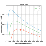
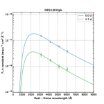
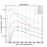
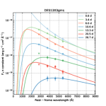
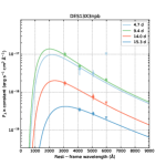
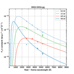
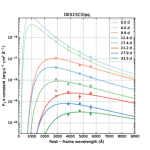
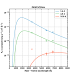
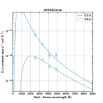
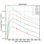
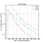
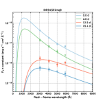
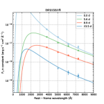
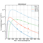
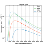
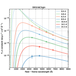
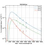
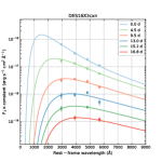
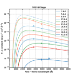
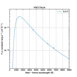
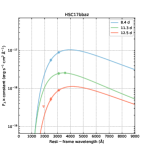
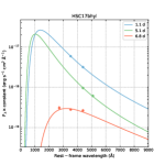
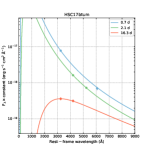
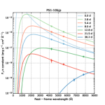
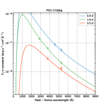
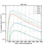
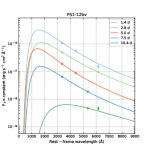
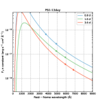
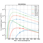
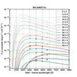
Figure 1: Fits to the multiepoch SEDs of 31 luminous REOTs using the blackbody model. The points are the photometry, while the solid lines are the model SEDs.

Since the derived physical properties of the REOTs of Drout et al. (2014) and Pursiainen et al. (2018) have not previously been presented, we repeat the blackbody fits for the SEDs of the 31 REOTs in Fig. 1. To get the best-fit parameters and the parameter ranges, we adopt the Markov Chain Monte Carlo (MCMC) method which is performed by using the emcee Python package (Foreman-Mackey et al., 2013). Once the MCMC is done, the best-fit values of the parameters are obtained by measuring the medians of the posterior samples. The uncertainties are computed to $3\sigma$ confidence. Our fits also show that the SEDs of almost all events can be fitted by the blackbody model. The best-fit values of the radii and the temperature, as well as the derived blackbody luminosities of the events, are shown in Table LABEL:tab:SED_Param_blackbody.

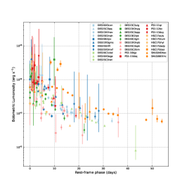
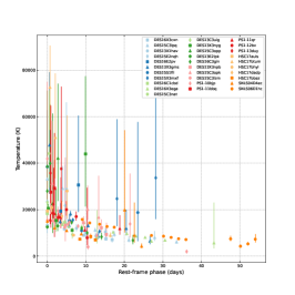
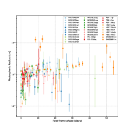
Figure 2: The derived bolometric light curves, the temperature evolution, and the radius evolution of the 31 luminous REOTs using the blackbody model.

To compare the photospheric properties of the luminous REOTs, we plot the their blackbody light curves, the temperature evolution, and the radius evolution in Fig. 2. It should be pointed out that the zero-point of time of every event is set to be their first detection, while the first point of every event in Fig. 2 corresponds to the epoch of the first SED. For some events, the multiband observations were performed a few days after the first detections.

Fig. 2 shows that, while the shapes of the events are homogeneous, the peak luminosities span from $\sim\,10^{43}$ erg s^-1 (comparable to the peak luminosities of SNe Ia) to $\sim\,5\,\times\,10^{44}$ erg s^-1 (brighter than some SLSNe). Additionally, the late-time temperatures of the events whose SEDs can be constructed at the epochs of $>\,10$ days no longer decline and reach a constant. For the events lacking SEDs at epochs of $>\,10$ days, the late-time temperature evolution is unknown. Finally, we find that the early-time radii of the photospheres of the events increased, and reached a “plateau” ($\sim$ (1–2) $\times 10^{15}$ cm) in most of events or even receded in some events.

4 Modeling the Multiband Light Curves of REOTs

In this section, we use the magnetar and CSI models to fit the multiband light curves of the events. The ejecta thermalize the input luminosities from the energy sources and produce the bolometric photosphere luminosities. The equations reproducing theoretical bolometric light curves are listed by Wang et al. (2015) and Dai et al. (2016) for the magnetar model, and by Chatzopoulos et al. (2012) and Wang et al. (2019) for the CSI models. Another assumption needed to calculate the multiband light curves of SNe or SN-like optical transients is that their photospheric emission can be described by the blackbody model or the absorbed blackbody model (Prajs et al., 2017; Nicholl et al., 2017). As shown in Fig. 1, the SEDs of the events in our sample are consistent with blackbody radiation and the blackbody assumption is valid at least at some epochs. We neglect the ultraviolet absorption effect, since the SEDs of the events we study can be fitted by the standard blackbody model. Finally, like Nicholl et al. (2017), we assume that the radii of the photospheres of the events were proportional to time at early epochs, while their temperatures no longer change at late epoches (see Eqs. (8) and (9) of Nicholl et al. 2017). Fig. 2 shows that the assumption of the “floor temperature” ($T_{\rm f}$) is valid for the events in our sample.

The value of the optical opacity ($\kappa$) of the ejecta depends on the SN type; it can be 0.05–0.20 cm² g^-1 for the ejecta of H-deficient SNe Ib/Ic/Ibn (see Wang et al. 2015, and the references therein). To reduce the number of the parameters, we assume that $\kappa=0.1$ cm² g^-1. For the CSI model, we suppose that the densities of the inner and outer components are respectively $\rho\,\propto\,r^{-1}$ and $\rho\,\propto\,r^{-7}$, and the density of the CSM is either $\rho\,\propto\,r^{-2}$ (a wind) or $\rho\,=$ constant (a shell). The definitions, units, and prior ranges of the free parameters of the two models are listed in Tables 3 and 4.

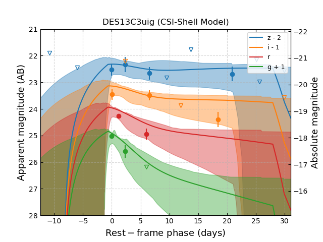
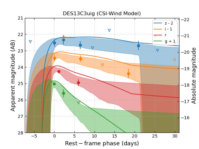
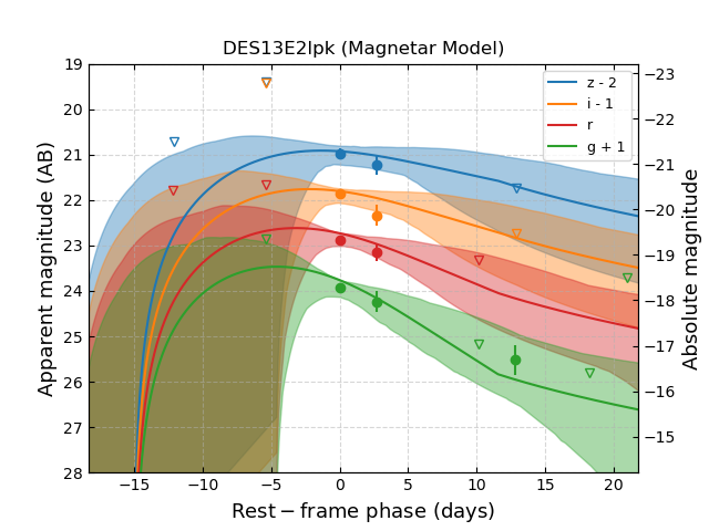
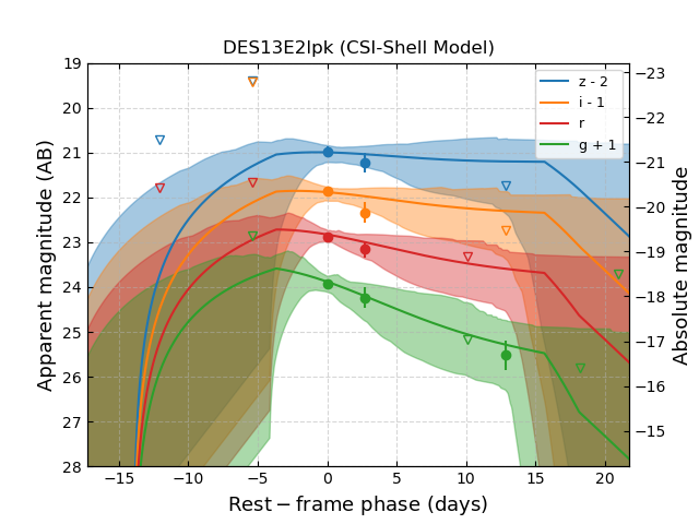
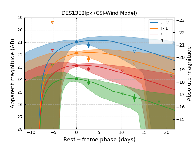
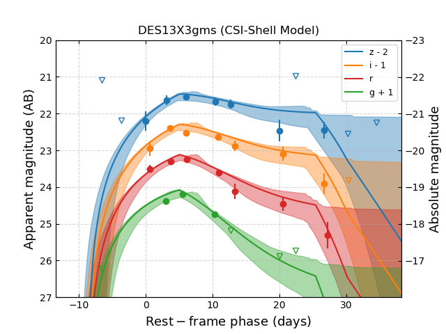
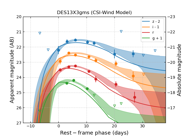
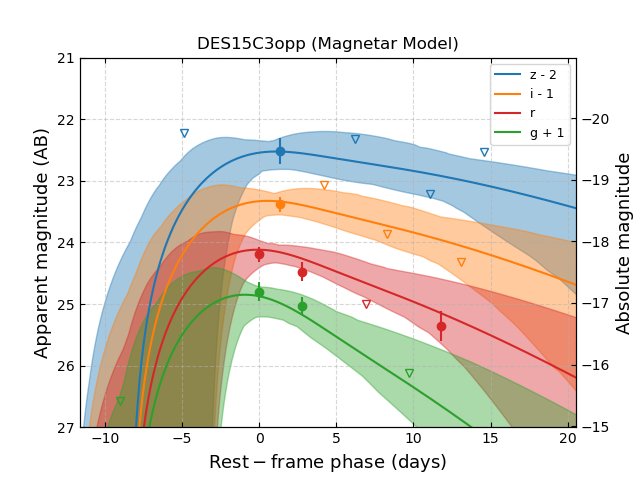
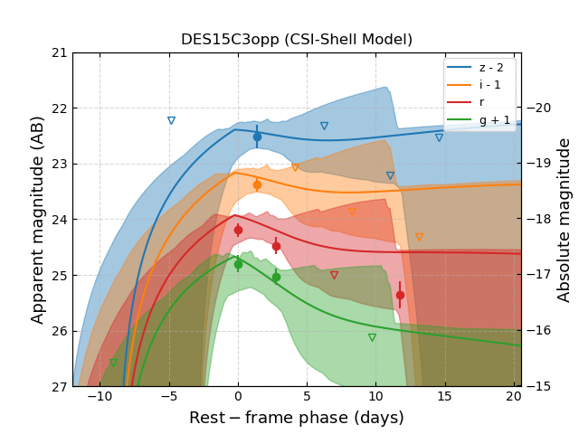
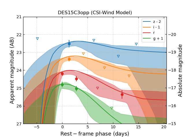
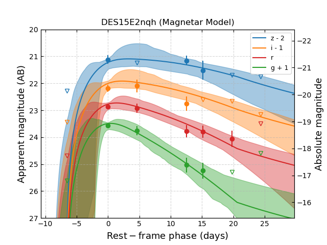
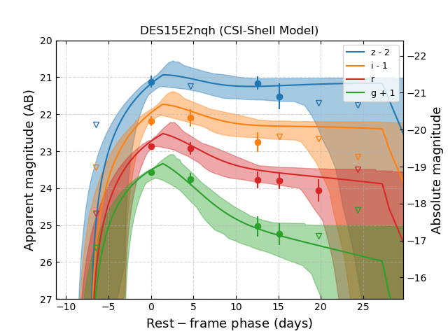
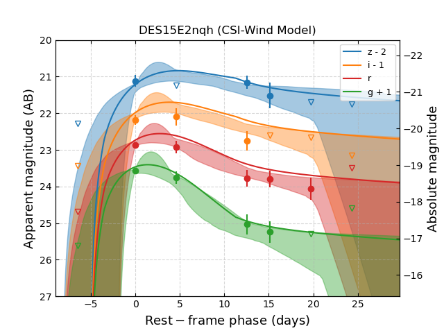
Figure 3: The fits for the multiband light curves of 20 REOTs using the magnetar model (left panels) and the CSI model (middle and right panels, which respectively correspond to the shell case and the wind case). The 20 REOTs can be fitted with excellent quality. The solid lines and the shaded regions present the best-fit light curves and $3\sigma$ uncertainties, respectively. The abscissa represents time since the explosion in the rest frame.

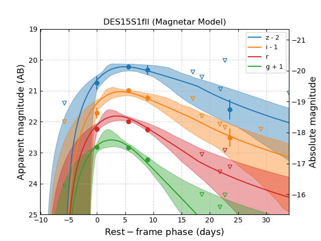
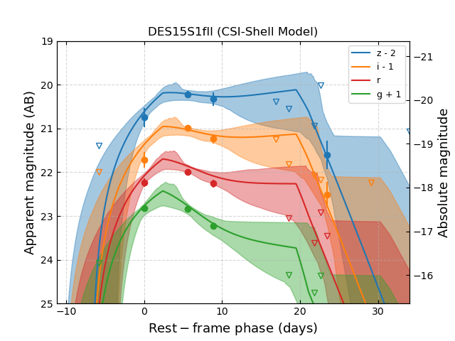
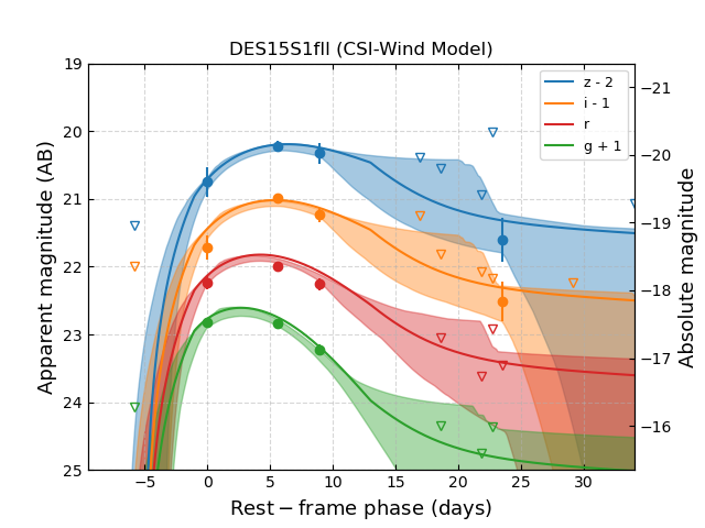
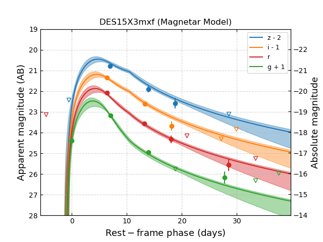
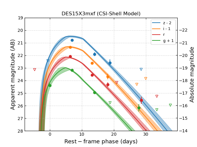
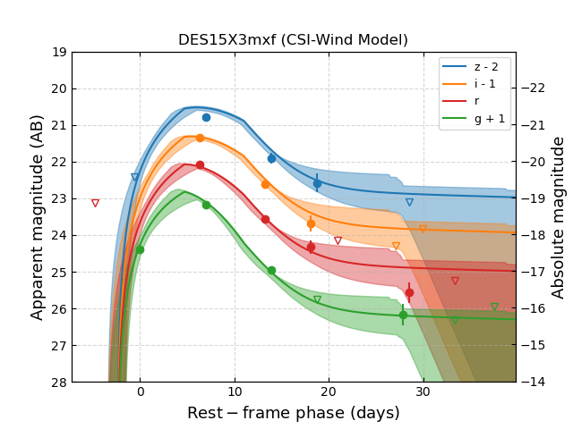
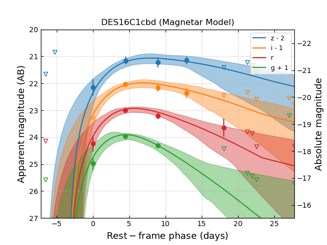
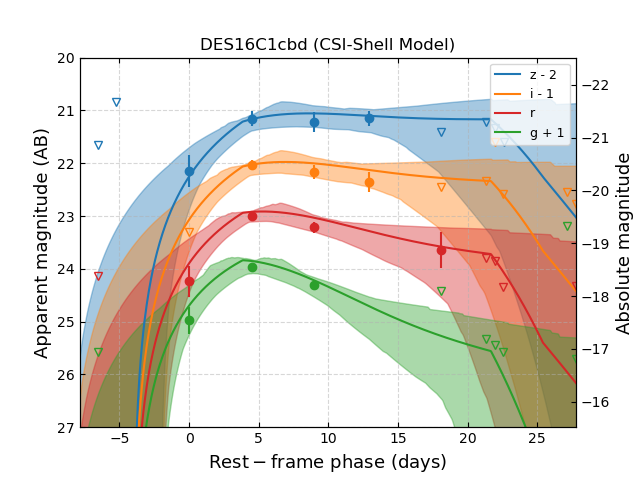
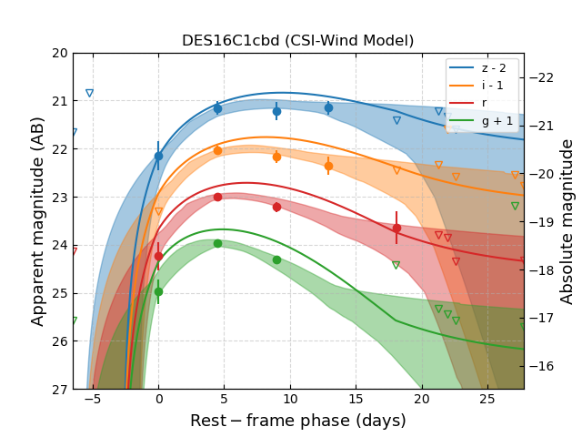
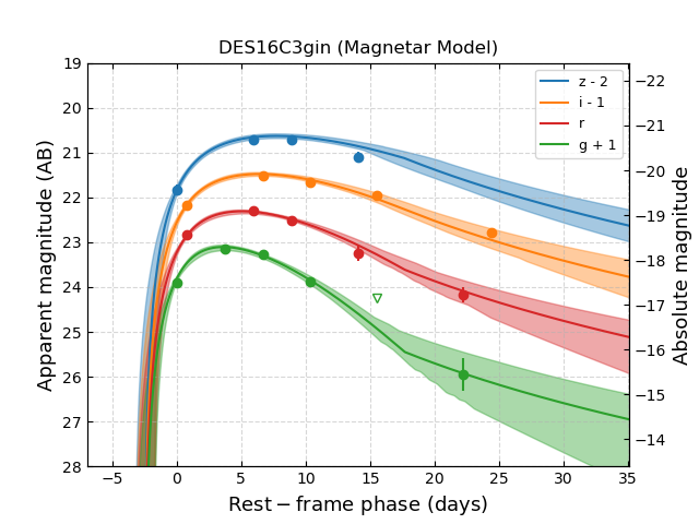
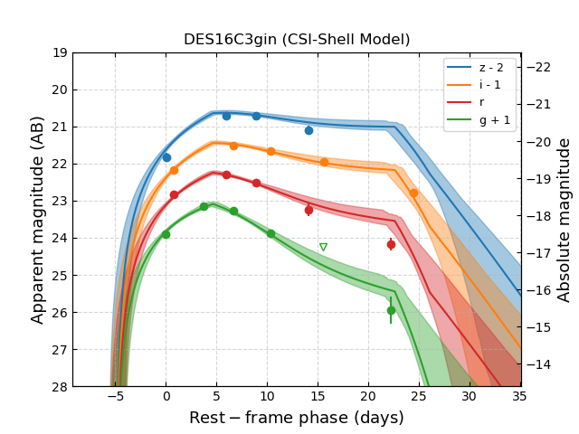
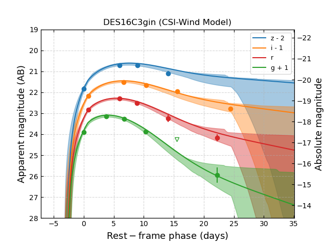
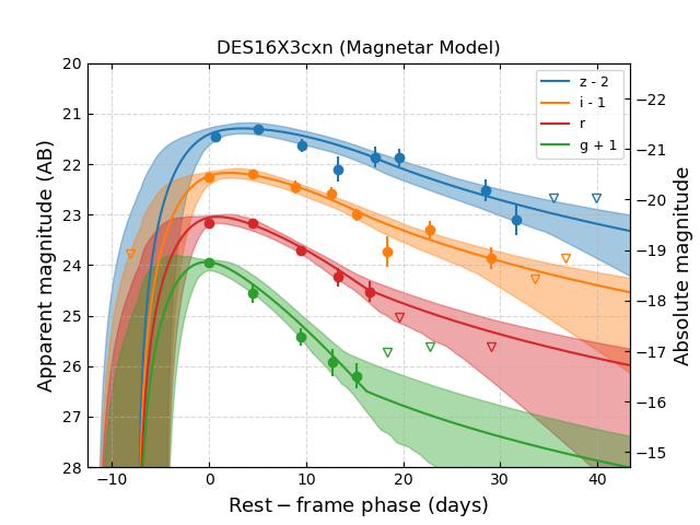
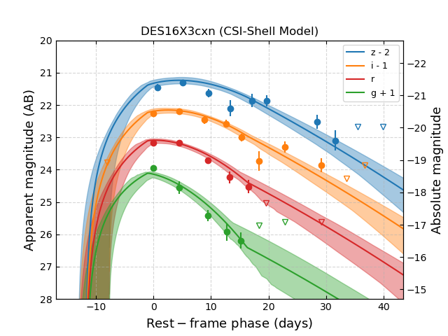
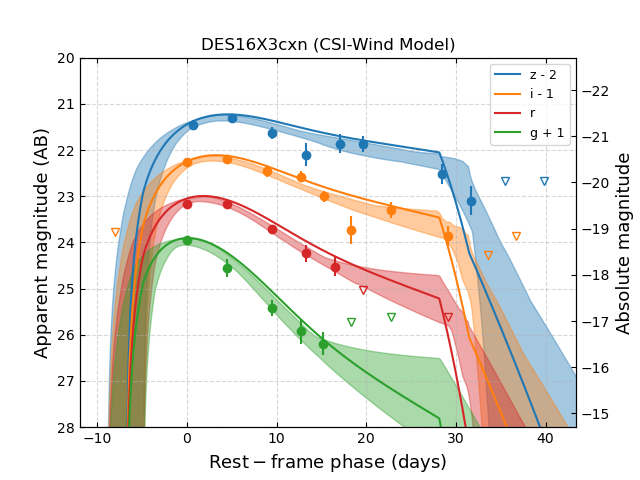
Figure 3: (Continued).

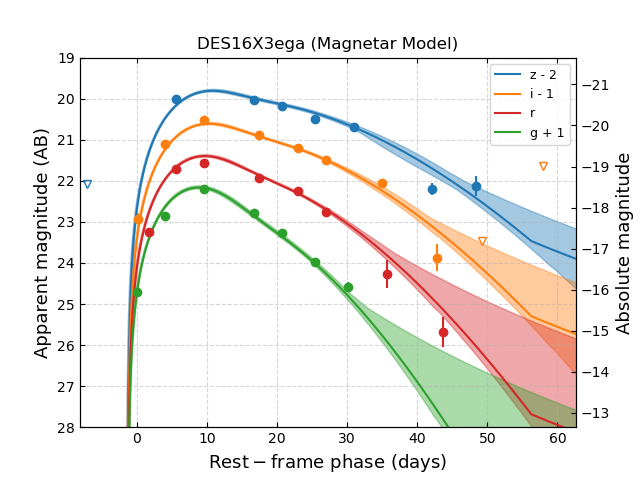
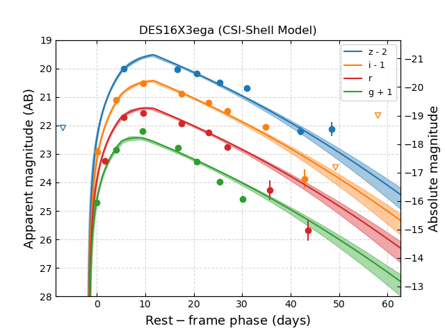
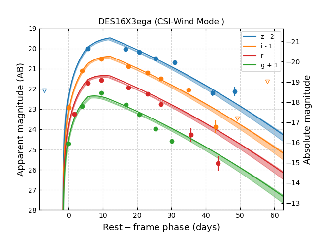
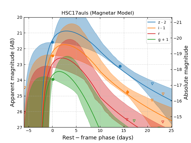
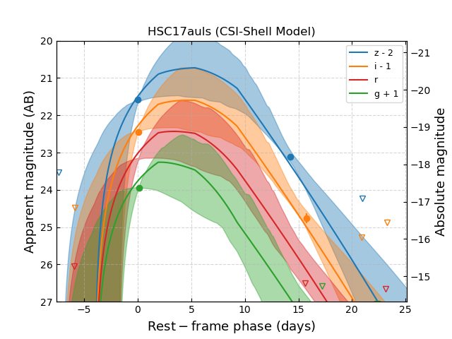
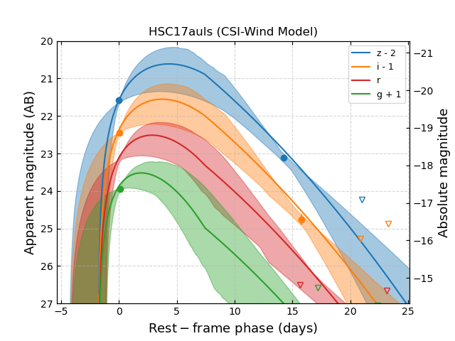
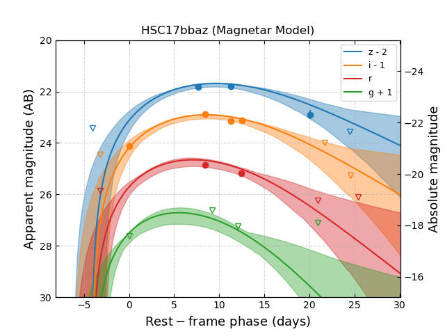
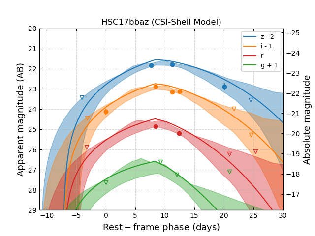
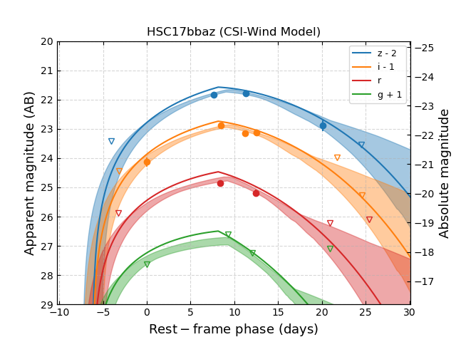
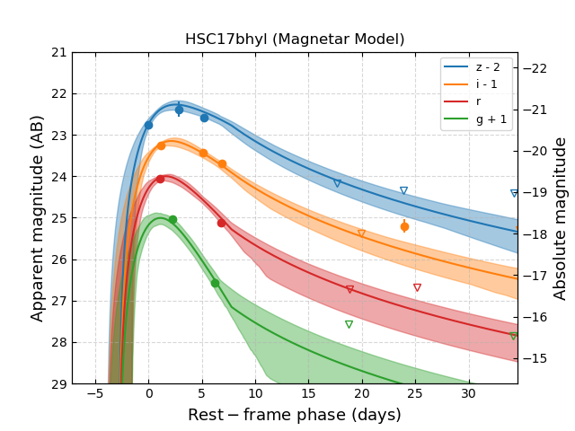
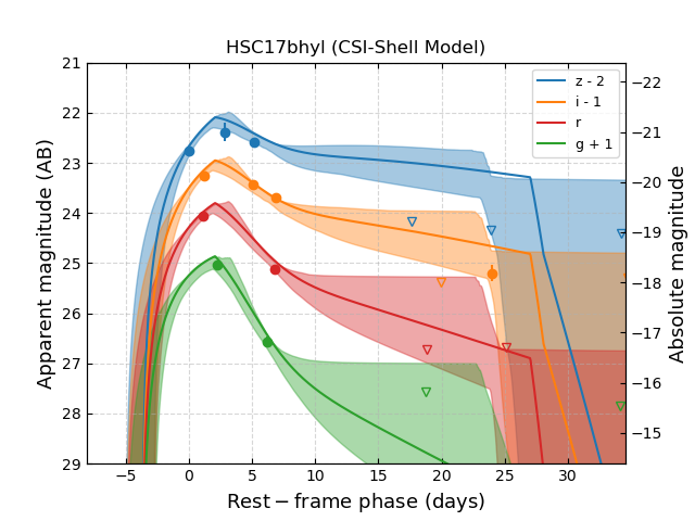
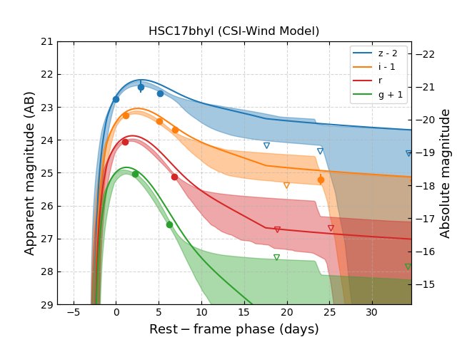
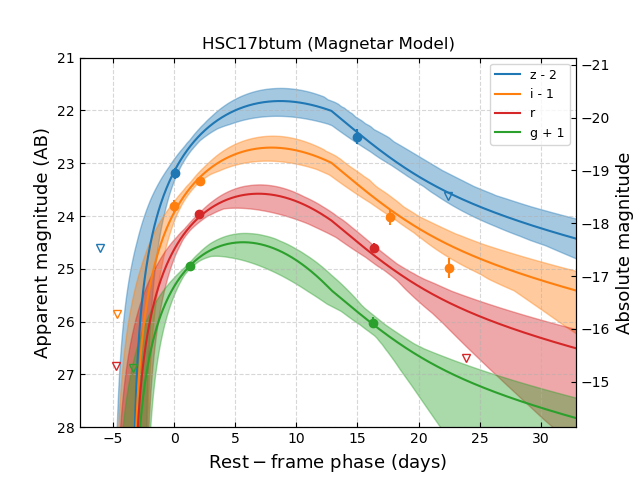
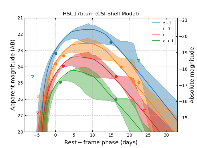
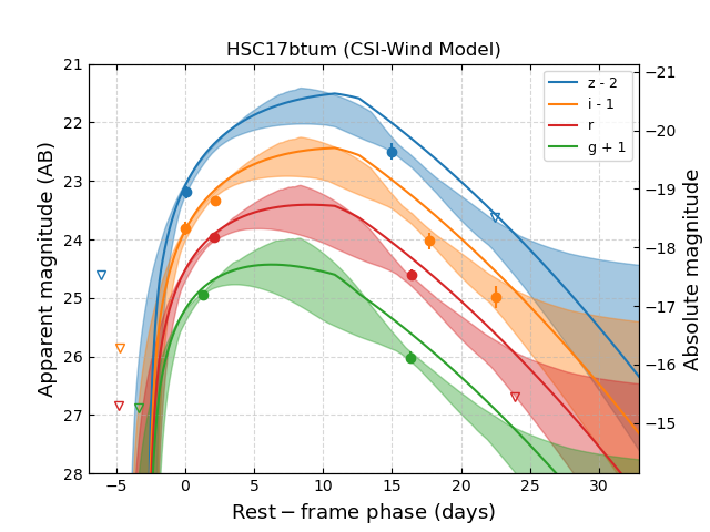
Figure 3: (Continued).

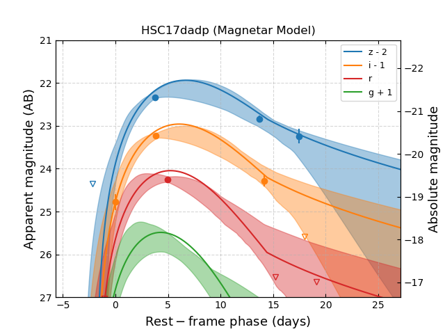
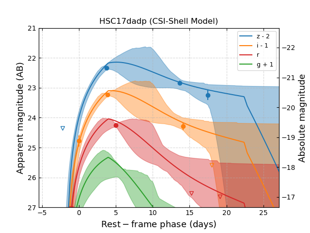
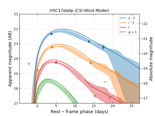
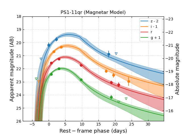
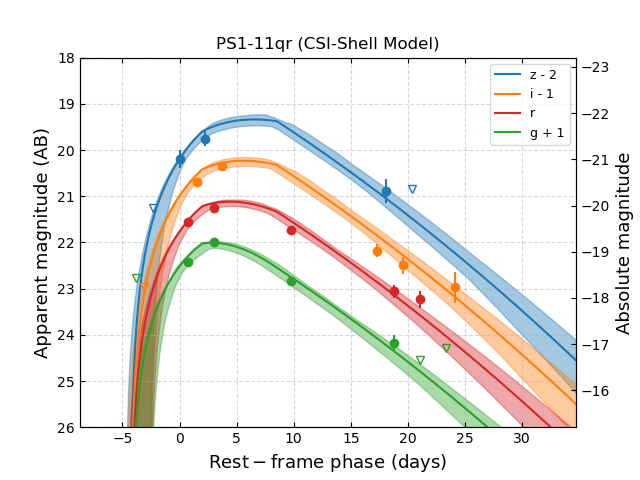
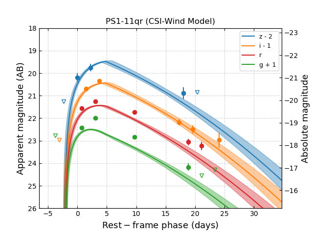
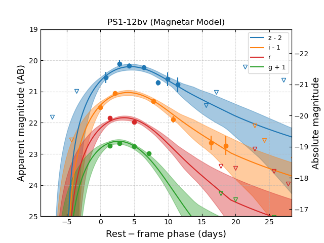
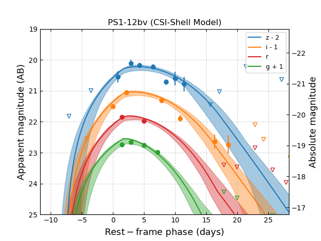
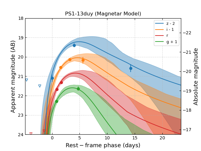
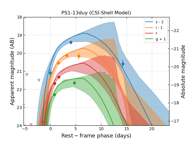
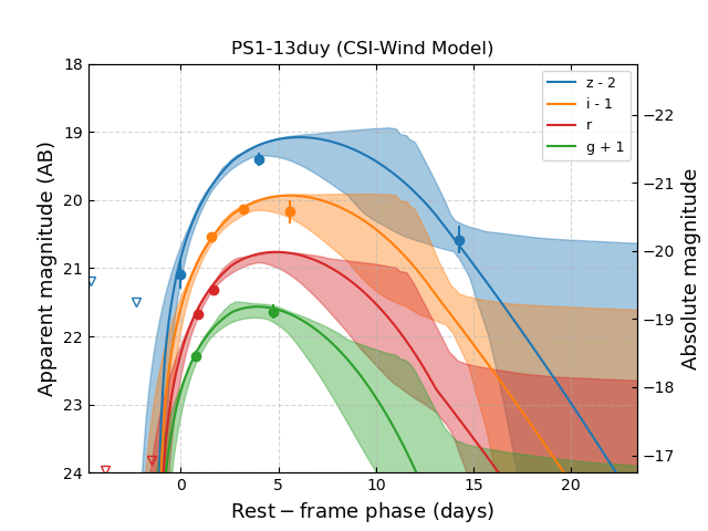
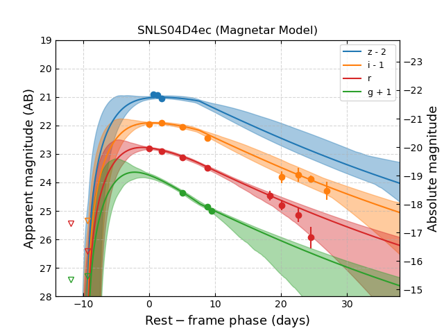
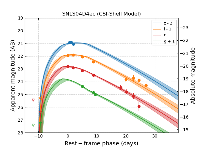
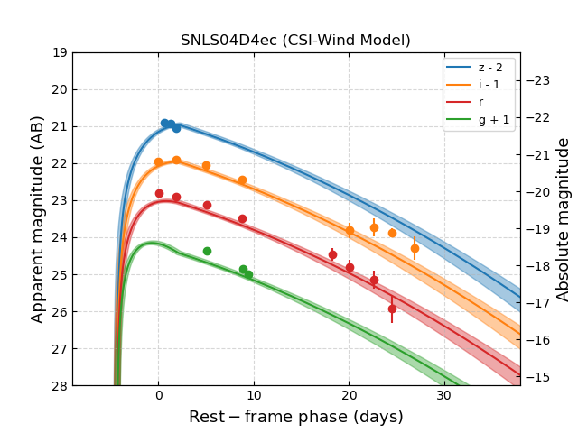
Figure 3: (Continued).

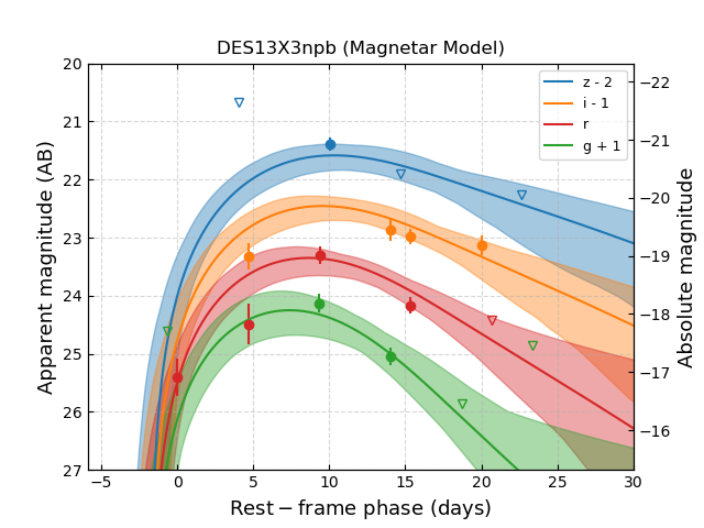
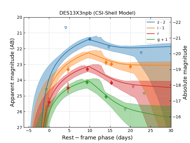
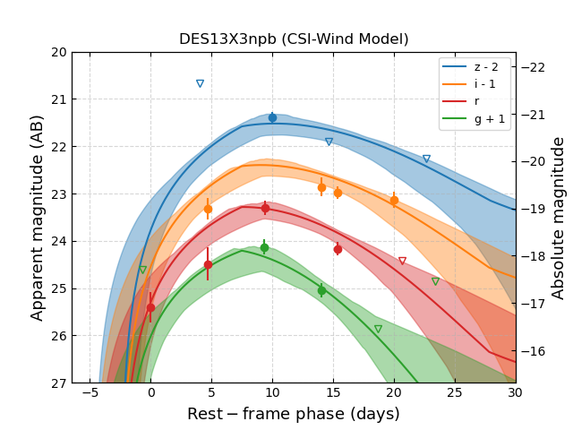
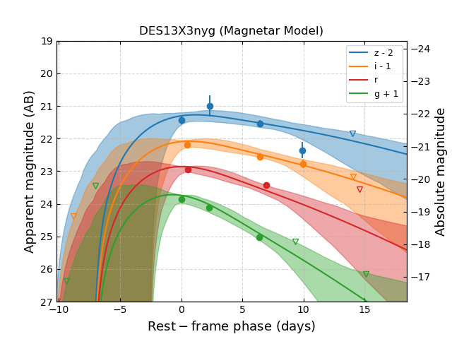
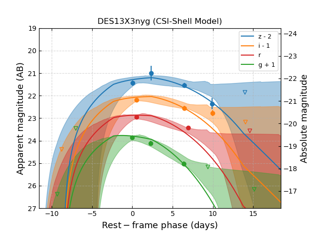
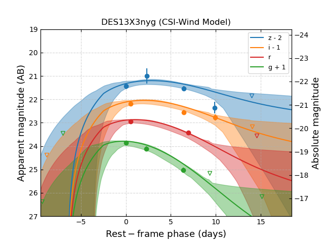
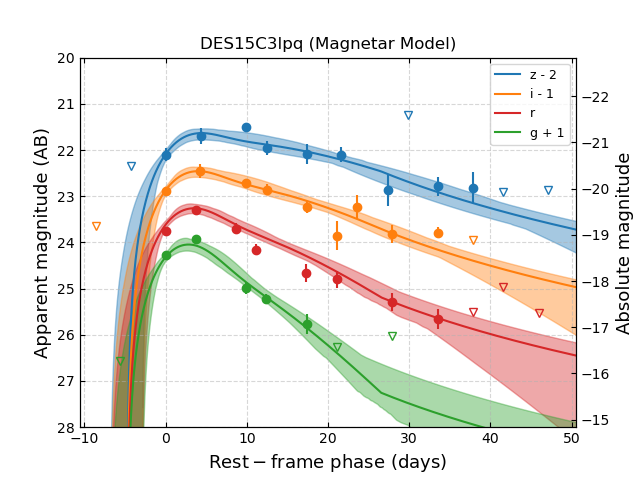
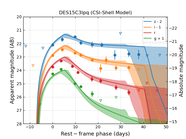
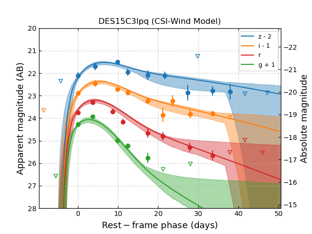
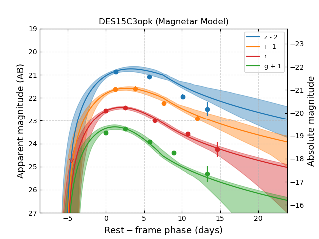
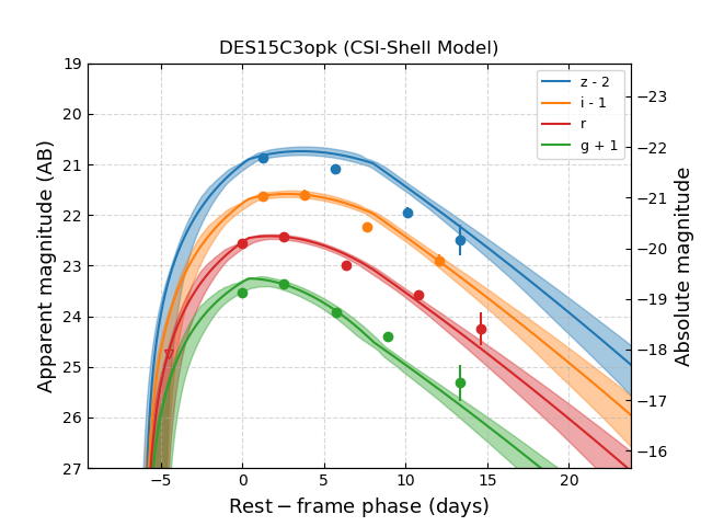
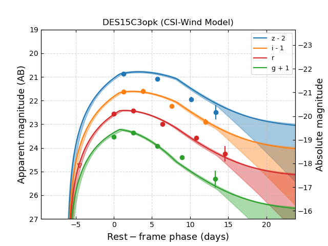
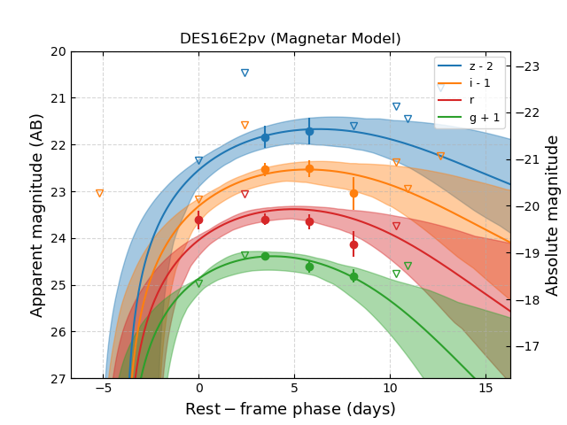
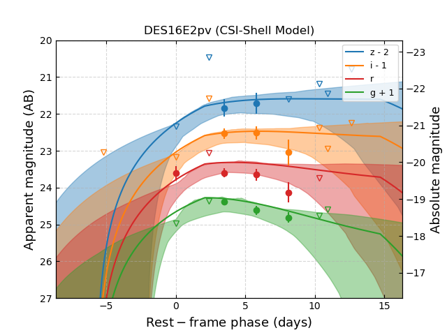
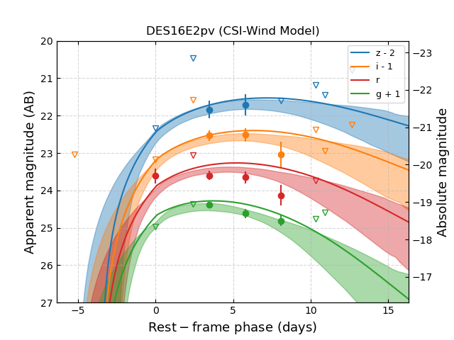
Figure 4: Same as Fig. 3, but for the 8 REOTs fitted with good quality.

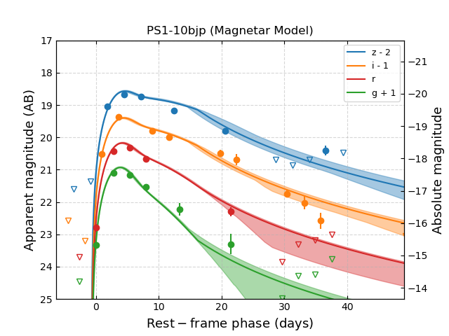
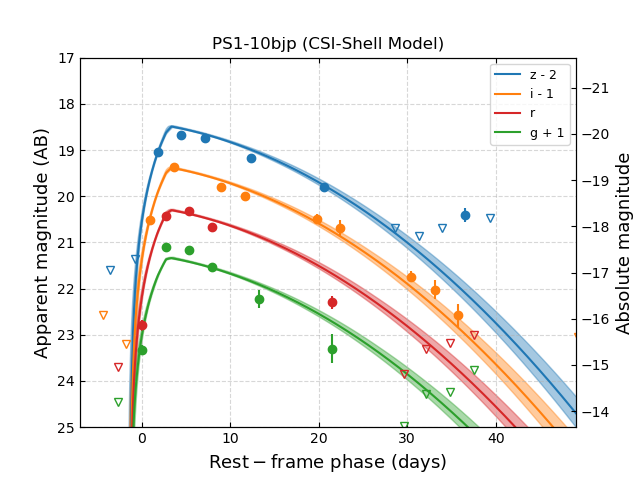
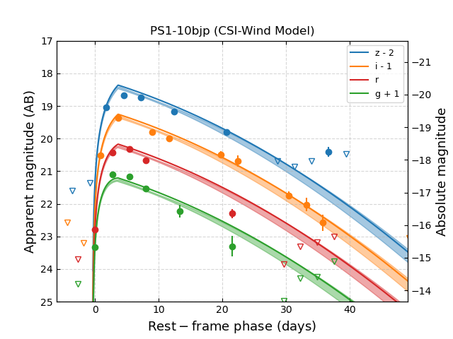
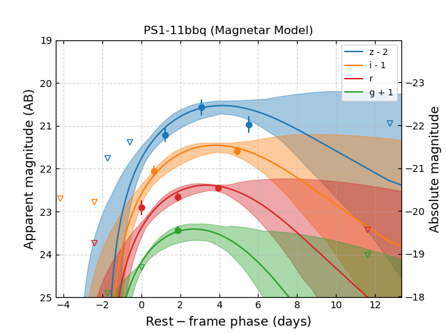
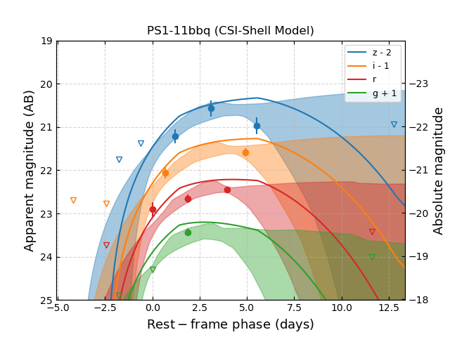
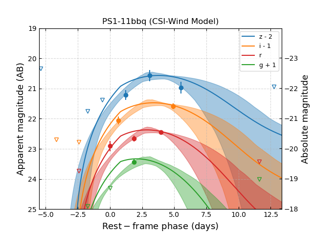
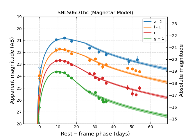
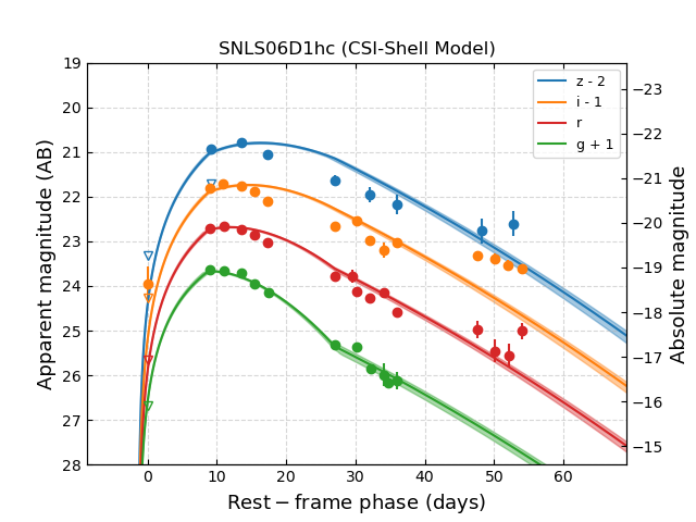
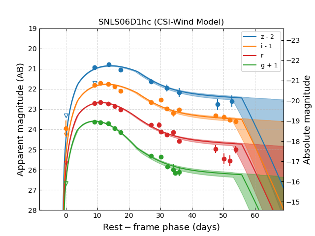
Figure 4: (Continued).

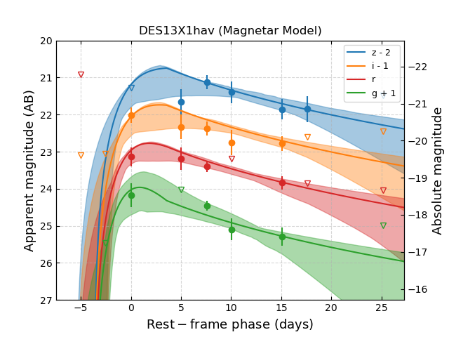
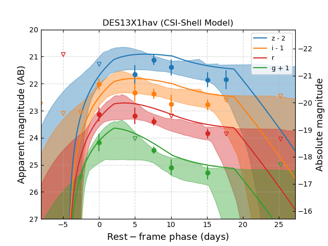
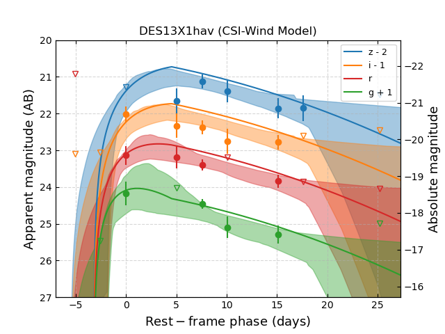
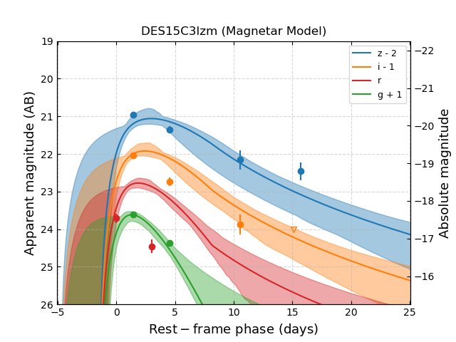
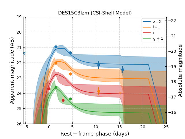
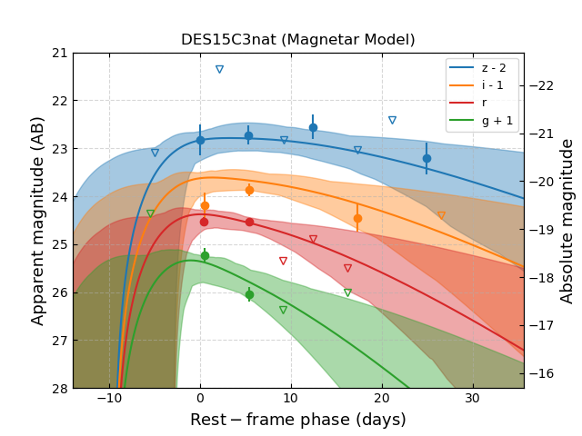
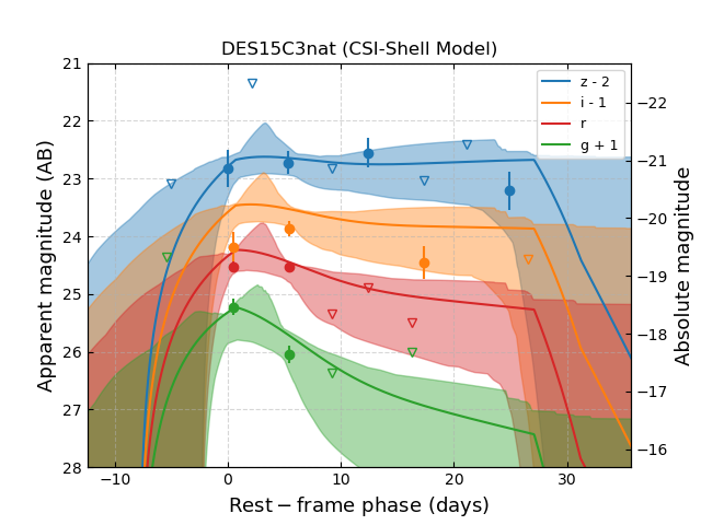
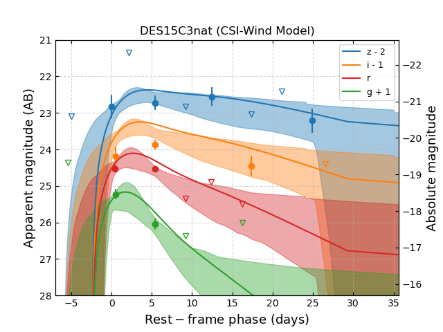
Figure 5: Same as Fig. 3, but for the 3 REOTs that cannot be fitted by the models.

The MCMC method is also used to get the best fits and derive the best-fit parameters of the models. Figures 3, 4, and 5 present the best fits of the magnetar (left panels), CSI-shell (middle panels), and CSI-wind (right panels) models. The corresponding best-fit parameters of the models are presented in Tables 5, 6, 7, respectively. The reduced $\chi^{2}$ values ($\chi^{2}$/dof; dof = degrees of freedom) are also listed in the Tables. The number of data points for some events is smaller than or equal to the number of parameters of the models, so the values of dof are $\leq\,0$ and $\chi^{2}$/dof is infinite or negative. For these cases, $\chi^{2}$/dof is meaningless, and we do not list the values.

We summarize the validity of the models we use in Table 8 and determine the best model for every event by comparing the $\chi^{2}$/dof values. We note that the $\chi^{2}$/dof values can be used to help determine the best model for an event, but they cannot be used to judge the validity of a model, since they strongly depend on the data error bars, the number of data points, and the number of free parameters in the model. The validity of a model are determined mainly by comparing the data and the best-fit light curves.

From the figures and the tables, we find the following.

1. 20 luminous REOTs can be fitted by the magnetar model with excellent quality (all data points are fitted by the theoretical light curves, or one/two data point(s) slightly deviate from the theoretical light curves); see the left panels of Fig. 3.

2. 8 REOTs can be fitted by the magnetar model with good quality (two or three data points slightly deviate from the theoretical light curves, but the major parts of the light curves can be fitted; or some data points deviate from the theoretical light curves, but can be supposed to be due to the cooling emission from the shock-heated extended envelopes (DES16E2pv) and/or late-rebrightening (SNLS06D1hc)); see the left panels of Fig. 4.

3. 25 REOTs can also be fitted by the CSI model; see the middle and right panels of Figures 3 and 4.

4. For the 25 REOTs that can fitted by both the magnetar and CSI models, the magnetar model get better fits than the CSI model do for all events.

5. The remaining 3 REOTs cannot be explained by both the the magnetar and CSI models (the data around the peaks cannot be fitted; see Fig. 5).

5 The Nature of REOTs

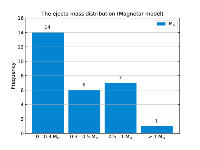
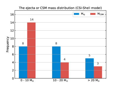
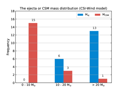
Figure 6: Histograms showing the distribution of the derived masses of the ejecta (and the derived CSM masses) for the magnetar model (top panel), the CSI-shell model (bottom-left panel), and the CSI-wind model (bottom-right panel).

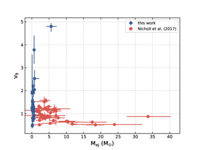
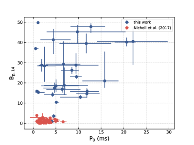
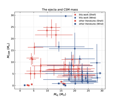
Figure 7: The $v$–$M_{\rm ej}$ space (top-left panel) and the $P_{0}$–$B_{p}$ space (top-right panel) of the magnetar model, and the $M_{\rm ej}$–$M_{\rm CSM}$ space (bottom panel) of the CSI model. Parameters are from Tables 5, 6, and 7. For comparison, the same parameters of SLSN I or SNe Ibn in the literature listed in 5 are also plotted.

In Section 4, we use the magnetar and CSI models to fit the multiband light curves of 31 luminous REOTs and find that 27 of them can be explained by the magnetar and/or the CSI model. The best-fit ejecta masses of 14, 6, 7, and 1 REOTs are 0.05–0.3 M_⊙, 0.3–0.5 M_⊙, 0.5–1.0 M_⊙, and $>1.0$ M_⊙, respectively (see Fig. 6). To illustrate the parameters, we present the four parameters ($M_{\rm ej}$, $v$, $B_{p}$, and $P_{0}$) of the models in Fig. 7; for comparison, the same parameters of SLSNe I that were supposed to be powered by magnetars (Nicholl et al., 2017) are also plotted. We find that the ejecta masses of luminous REOTs are significantly smaller than those of the magnetar-powered SLSNe I, except for HSC17bbaz ($M_{\rm ej}=5.58^{+1.6}_{-1.4}$ M_⊙). On the other hand, the velocity of the ejecta of some luminous REOTs is larger than that of the magnetar-powered SLSNe I. Furthermore, the $B_{p}$–$P_{0}$ distribution of the REOTs is significantly larger than that of the magnetar-powered SLSNe I.

If mass transfer in a binary system consisting of a helium star and a compact companion (e.g., a neutron star; NS, hereafter) strips the helium star, the star would became a stripped core and explode as an ultrastripped CCSN with ejecta mass $\sim 0.1$–0.3 M_⊙ (Tauris et al., 2013; Suwa et al., 2015; Tauris et al., 2015; Moriya & Eldridge, 2016; Moriya et al., 2017). By providing a detailed example, Tauris et al. (2013) demonstrated that the mass-transfer process in a binary consisting of an NS and a helium star can produce a small, bare core of $\sim 1.5$ M_⊙ that collapses and produces an SN whose ejecta mass is only $\sim 0.1$ M_⊙.

If the explosion leaves a normal NS, the SN would be rather faint since the ⁵⁶Ni yield must be less than the ejecta mass. Drout et al. (2013) and Tauris et al. (2013) used the ⁵⁶Ni-powered (Arnett, 1982) ultrastripped SN model (Tauris et al., 2013, 2015; Moriya & Eldridge, 2016; Moriya et al., 2017) to explain the pseudobolometric light curve of SN 2005ek. De et al. (2018) reported photometric and spectral observations of iPTF14gqr, a rapidly evolving SN Ic. By modeling the bolometric light curve and analyzing the spectra, De et al. (2018) found that the early-time excess can be explained by the post-shock cooling model involving an extended He-rich envelope heated by the SN shock, and the second peak of the SN can be explained by the radioactivity model with $M_{\rm ej}\approx 0.15$–0.30 M_⊙ and $M_{\rm Ni}\approx 0.05$ M_⊙. Yao et al. (2020) studied SN 2019dge, a rapidly evolving SN Ib, and found that its ejecta mass is also extremely low, $\sim\,0.3$ M_⊙. It can be expected that the rapidly evolving subluminous SNe IIb/Ib/Ic of Ho et al. (2021) might also be ⁵⁶Ni-powered ultrastripped CCSNe.

If the ultrastripped CCSNe create rapidly rotating magnetars, the energy input from the newly-born magnetar would significantly boost the luminosities of the SNe, producing (super)luminous REOTs/SNe whose peak luminosities can be significantly larger than those of SN 2005ek, iPTF14gqr, SN 2019dge, and other similar events. To date, there are only two luminous, rapidly evolving SNe Ic — iPTF16asu and SN 2018gep. Whitesides et al. (2017) used four different models (⁵⁶Ni, magnetar, off-axis afterglow, and post-shock cooling) to fit the pseudobolometric light curves of the luminous SN Ic-BL iPTF16asu, suggesting that all of them cannot fit the whole light curve well. Wang et al. (2019) used more complicated models (magnetar plus interaction model, etc.) to fit the bolometric light curve of iPTF16asu. Pritchard et al. (2021) used ⁵⁶Ni, ⁵⁶Ni plus magnetar, and ⁵⁶Ni plus CSI models to fit the multiband light curves of SN 2018gep, demonstrating that the last model is the best one for explaining the data. All of these works require additional energy sources to yield the extraordinary luminosities of the luminous, rapidly evolving SNe Ic-BL. Our fits suggest that some luminous REOTs might be luminous, rapidly evolving SNe Ib/Ic similar to iPTF16asu and SN 2018gep. Moreover, we demonstrate that some luminous REOTs might be luminous (ultra)stripped CCSNe powered by the nascent magnetars.

Our fits also show that 25 luminous REOTs can be explained by the CSI model. We find that, if they were powered by CSI, the derived masses of the ejecta and the CSM can be rather large, $\sim 3$–30 M_⊙ and $\sim 2.6$–30 M_⊙ (respectively). For the CSI-shell model, the respective derived ejecta masses of 8, 8, and 6 events are $\sim 3$–10 M_⊙, $\sim 10$–20 M_⊙, and $\sim 20$–30 M_⊙; for the CSI-wind model, the respective derived ejecta masses of 0, 6, and 13 events are $\sim 3$–10 M_⊙, $\sim 10$–20 M_⊙, and $\sim 20$–30 M_⊙ (see Fig. 6 for the mass distribution). As shown in Fig. 7, the masses of the ejecta are consistent with that of SNe Ibn ($\sim 2$–20 M_⊙). The mean values of the derived CSM masses are larger than the values quoted in the literature (see, e.g., Karamehmetoglu et al. 2017, Vallely et al. 2018, Gangopadhyay et al. 2020, Wang & Li 2020, Kool et al. 2020, Xiang et al. 2021), but the CSM masses of some events are lower than $\sim 5$ M_⊙. Moreover, the sample of SNe Ibn fitted by the CSI model is too small, and we can expect that modeling of a larger sample might extend the range of the CSM masses of SNe Ibn. We therefore suggest that the derived masses of the ejecta and the CSM favor the scenario that some events might be luminous SNe Ibn/IIn which are so-called “interacting SNe” exploding in massive, dense CSM.

The resemblance between the light curves of REOTs we study here and the roughly dozen rapidly evolving SNe Ibn presented by Ho et al. (2021) can provide additional support for the scenario that at least some luminous REOTs might be interacting SNe. Although the values of $\chi^{2}$/dof of the CSI model for some events are larger than that of the magnetar model for the same events, we cannot conclude that the magnetar model is the best model for them, since some luminous REOTs might be luminous SNe Ibn/IIn for which the CSI model is best.

6 Conclusions

In this paper, we collect 31 luminous REOTs which cannot be explained by the ⁵⁶Ni model that has long been adopted to account for the light curves of SNe Ia and normal SNe Ibc. We suppose that the REOTs are either luminous ultrastripped CCSNe or SNe Ibn/IIn, and we use the magnetar and CSI models to fit their multiband light curves.

We find that 28 events in the sample can be explained by the magnetar model; the best-fit ejecta masses of 14, 6, 7, and 1 of them are (respectively) 0.05–0.3 M_⊙, 0.3–0.5 M_⊙, 0.5–1.0 M_⊙, and $>1.0$ M_⊙, indicating that most REOTs are ultrastripped SNe ($\sim 0.05$–0.20 M_⊙; Tauris et al. 2013) or stripped SNe if they were powered by the magnetars. The ejecta masses of the 6 REOTs with masses $\sim 0.5$–1.0 M_⊙ are comparable to that of the Type Ic SN 1994I ($0.6^{+0.3}_{-0.1}$ M_⊙), while the derived mass of HSC17bbaz ($5.58^{+1.6}_{-1.4}$ M_⊙) is comparable to that of SLSNe I studied by Nicholl et al. (2017). Our modeling assumes that the value of the optical opacity is 0.1 cm² g^-1; adopting smaller values for the optical opacity (e.g., 0.05 cm² g^-1), the inferred masses would be larger, since the derived ejecta mass is inversely proportional to the optical opacity (see, e.g., Wang et al. 2015; Lyman et al. 2016).

In addition, our modeling shows that 25 REOTs can be fitted by the CSI model, all of which can also be explained by the magnetar model. The magnetar model can provide better fits than the CSI model for all events that can be explained by both models. The remaining three events in our sample cannot be explained by either of the models. Although the fitting quality of the CSI model for most of the luminous REOTs that can explained by both of the models is lower than that of the magnetar model, we cannot exclude the CSI model since a fraction of them might be luminous SNe Ibn/IIn that favor the CSI model. Moreover, the derived ejecta masses of the events that can be fitted by the CSI model are consistent with that of some SNe Ibn, supporting the scenario that some luminous REOTs might be luminous rapid evolving SNe Ibn.

The resemblance between the rapidly evolving multiband light curves of the luminous REOTs and those of some luminous rapidly evolving SNe Ic (iPTF16asu and SN 2018gep) and SNe Ibn also indicates that some of our luminous REOTs might be luminous SNe Ib/Ic or SNe Ibn/IIn. Therefore, we suggest that both the magnetar and the CSI models are plausible in explaining the luminous REOTs.

Unfortunately, the luminous REOTs we study are spectroscopically unclassified, preventing us from drawing more robust conclusions about their nature. Future high-cadence sky surveys, together with follow-up photometric and spectroscopic observations of luminous REOTs, might permit detailed modeling of their multiband light curves, giving more stringent constraints on their physical properties and helping to distinguish among different models. The spectra of luminous REOTs would provide key information for determining their nature and the energy sources. If the spectral classifications show that luminous REOTs are SNe Ibn/IIn or SNe Ib/Ic, then they would favor the CSI model or the magnetar-powered (ultra)stripped CCSN model, respectively.

The Large Synoptic Survey Telescope (LSST; Ivezic et al. 2008; LSST Science Collaborations 2009) can discover $\sim 100,000$ SNe II per year (LSST Science Collaborations, 2009); since the rate of SNe Ibc is $\sim 1/3$ that of SNe II (see Table 1 of Smartt 2009, and references therein), $\sim 130,000$ CCSNe should be discovered each year by LSST. Drout et al. (2014) find that the rate of REOTs is 4–7% of the CCSN rate at redshift $z\approx 0.2$; based on the 37 DES REOTs with spectroscopic redshifts, Pursiainen et al. (2018) estimate that the REOT rate is $\gtrsim 1000$ Gpc^-3 yr^-1, which is 1.5% of the CCSN rate derived by Li et al. (2011). As noted by Pursiainen et al. (2018), this value is only a lower limit; adding 35 DES REOTs that do not have spectroscopic redshifts, the rate would be doubled to 3% of the CCSN rate. We adopt the latter value as a conservative lower limit to estimate the LSST REOT discovery rate, finding that $\gtrsim 4000$ REOTs should be discovered by LSST per year. According to the PS1 and DES REOT samples, the ratio of luminous REOTs to all discovered REOTs is $\sim 70$% (for the PS1 sample) or $\sim 75$% (for the DES sample); thus, the number of luminous REOTs that should be discovered by LSST is $\sim 3000$ per year. It can be expected that further investigation of a significantly larger sample might provide more reliable values of the ratios of luminous REOTs that can and cannot be explained by the magnetar or CSI models.

Table 1: Basic information for the REOTs and their host galaxies in our sample.^a

Name	$\alpha$	$\delta$	$z$	$M_{\rm rest,peak,g}$		SFR	sSFR	Offset	$E_{\mathrm{B-V}}$
	(J2000)	(J2000)		(mag)		($M_{\odot}$ yr-1)	(Gyr-1)	(kpc)	(mag)
DES13C3uig	03:31:46.55	$-$27:35:07.96	0.67	$-19.00\pm 0.08$		$\sim$11.2	$\sim$0.26	3.80	0.007
DES13E2lpk	00:40:23.80	$-$43:32:19.74	0.48	$-19.19\pm 0.07$		$\sim$6.17	$\sim$0.42	4.77	0.0054
DES13X1hav	02:20:07.80	$-$05:06:36.53	0.58	$-19.42\pm 0.32$		$\sim$0.68	$\sim$0.48	2.51	0.0186
DES13X3gms	02:23:12.27	$-$04:29:38.35	0.65	$-19.66\pm 0.04$		$\sim$1.15	$\sim$0.68	6.09	0.0257
DES13X3npb	02:26:34.11	$-$04:08:01.96	0.50	$-19.01\pm 0.16$		$\sim$14.13	$\sim$0.31	1.06	0.0245
DES13X3nyg	02:27:58.17	$-$03:54:48.05	0.71	$-20.26\pm 0.05$		$\sim$0.95	$\sim$0.83	2.95	0.0224
DES15C3lpq	03:30:50.89	$-$28:36:47.08	0.61	$-19.84\pm 0.08$		$\sim$0.81	$\sim$0.48	2.18	0.0077
DES15C3lzm	03:28:41.86	$-$28:13:54.96	0.33	$-18.54\pm 0.04$		$\sim$2.57	$\sim$0.36	2.43	0.0059
DES15C3nat	03:31:32.44	$-$28:43:25.06	0.84	$-19.37\pm 0.14$		$\sim$3.24	$\sim$0.46	4.52	0.0087
DES15C3opk	03:26:38.76	$-$28:20:50.12	0.57	$-20.20\pm 0.04$		$\sim$2.34	$\sim$0.34	3.41	0.0125
DES15C3opp	03:26:57.53	$-$28:06:53.61	0.44	$-18.11\pm 0.15$		$\sim$0.38	$\sim$0.42	2.44	0.0081
DES15E2nqh	00:38:55.59	$-$43:05:13.14	0.52	$-19.74\pm 0.06$		$\sim$0.44	$\sim$0.48	3.22	0.0077
DES15S1fll	02:51:09.36	$-$00:11:48.71	0.23	$-18.23\pm 0.05$		$\sim$0.68	$\sim$0.36	11.01	0.0547
DES15X3mxf	02:26:57.72	$-$05:14:22.81	0.44	$-19.64\pm 0.02$		$\sim$0.89	$\sim$0.42	9.81	0.0235
DES16C1cbd	03:39:25.97	$-$27:40:20.37	0.54	$-19.46\pm 0.05$		-	-	6.83	0.0100
DES16C3gin	03:31:03.06	$-$28:17:30.98	0.35	$-19.15\pm 0.03$		$\sim$1.32	$\sim$0.36	7.93	0.0085
DES16E2pv	00:36:50.19	$-$43:31:40.16	0.73	$-19.84\pm 0.08$		$\sim$2.51	$\sim$0.41	7.85	0.0055
DES16X3cxn	02:27:19.32	$-$04:57:04.27	0.58	$-19.62\pm 0.05$		$\sim$1.07	$\sim$0.48	4.12	0.0236
DES16X3ega	02:28:23.71	$-$04:46:36.18	0.26	$-19.25\pm 0.03$		$\sim$3.80	$\sim$0.36	8.93	0.0302
HSC17auls	09:57:55.13	+02:25:08.10	0.339	$-18.00\pm 0.02$		-	1.19	3.73	0.0176
HSC17bbaz	09:58:26.32	+00:53:08.09	1.480	$-19.76\pm 0.11$($i$)		-	8.23	25.69	0.0233
HSC17bhyl	10:01:22.21	+02:01:53.37	0.750	$-18.69\pm 0.04$		-	1.69	0.43	0.0156
HSC17btum	09:57:54.02	+02:39:57.17	0.467	$<-17.73\pm 0.05$		-	0.51	13.01	0.0168
HSC17dadp	10:00:29.05	+01:36:27.66	0.830	$-18.74\pm 0.03$($i$)		-	0.39	5.27	0.0161
PS1-10bjp	23:26:21.402	$-$01:31:23.11	0.113	$-$18.2		$\sim$2.1	$\sim$1.6	2.39	0.0483
PS1-11bbq	08:42:34.733	+42:55:49.61	0.646	$-$19.6		$>$0.3	$>$2.4	8.81	0.026
PS1-11qr	09:56:41.767	+01:53:38.25	0.324	$-$19.5		$\sim$4.3	$\sim$0.3	12.58	0.0164
PS1-12bv	12:25:34.602	+46:41:26.97	0.405	$-$19.4		$>$0.3	$>$0.03	10.29	0.0102
PS1-13duy	22:21:47.929	$-$00:14:34.94	0.270	$-$18.6		$>$0.1	$>$0.2	2.16	0.0548
SNLS04D4ec	22:16:29.29	$-$18:11:04.1	0.593	$-19.21\pm 0.02$		$2.87\pm 0.82$(OII)	$\sim$0.44	-	0.0238
SNLS06D1hc	02:24:48.25	$-$04:56:03.6	0.555	$-19.75\pm 0.01$		$0.21\pm 0.07$(OII)	$\sim$0.36	-	0.0244

^a Except for the values of the Milky Way extinction ($E_{\mathrm{B-V}}$), which are from Schlafly & Finkbeiner (2011), all information comes from Tables 3, 4, and 7 of Pursiainen et al. (2018), Tables 1, 2, and 3 of Tampo et al. (2020), Tables 1 and 5 of Drout et al. (2014), and Tables 1, 6, and 8 of Arcavi et al. (2016). Note that the values of SFR and sSFR of the host galaxies of DES REOTs are obtained by using the values of log($M_{\star}$/$M_{\odot}$) and log(sSFR) listed in Table 7 of Pursiainen et al. (2018), the values of sSFR of the host galaxies of SNSL04D4ec and SNLS06D1hc are obtained from the values of log(sSFR) listed in Table 7 of Arcavi et al. (2016), the $g$-band peak magnitudes of HSC REOTs are derived from the $i$-band peak magnitudes listed in Table 2 of Tampo et al. (2020) and the photometry presented in Table 4 of Tampo et al. (2020), and the $g$-band peak magnitudes of SNSL04D4ec and SNLS06D1hc are derived from the $z$- and $i$-band peak magnitudes listed in Table 6 of Arcavi et al. (2016) and the photometry presented in Table 2 of Arcavi et al. (2016).

Table 2: Best-fit parameters of the blackbody model for REOT SEDs.

Name	Phase	$T_{\rm ph}$	$R_{\rm ph}$	$L_{\rm ph}$	$\chi^{\rm 2}$
	(days)	($10^{3}$ K)	($10^{15}$ cm)	($10^{42}$ erg s-1)
DES13C3uig	0.0	$23.11^{+6.3}_{-3.8}$	$0.46^{+0.1}_{-0.1}$	$42.7^{+25.3}_{-11.2}$	0.67
	2.3	$12.83^{+5.9}_{-2.4}$	$0.9^{+0.4}_{-0.4}$	$16.83^{+6.1}_{-3.4}$	0.34
	6.5	$9.25^{+3.1}_{-1.7}$	$1.34^{+0.7}_{-0.5}$	$9.88^{+2.0}_{-1.3}$	0.97
DES13E2lpk	0.0	$12.56^{+1.0}_{-0.8}$	$1.28^{+0.1}_{-0.1}$	$29.16^{+2.5}_{-2.1}$	0.79
	2.7	$12.99^{+3.4}_{-2.2}$	$1.05^{+0.3}_{-0.3}$	$22.37^{+8.6}_{-4.5}$	0.64
DES13X1hav	0.0	$13.29^{+6.9}_{-3.4}$	$1.32^{+0.9}_{-0.6}$	$39.82^{+30.7}_{-9.0}$	0.39
	5.0	$28.68^{+37.5}_{-15.1}$	$0.53^{+0.6}_{-0.2}$	$135.07^{+1009.9}_{-104.3}$	0.23
	7.6	$11.97^{+1.7}_{-1.3}$	$1.4^{+0.3}_{-0.3}$	$29.09^{+3.7}_{-2.8}$	2.18
	10.0	$10.03^{+2.7}_{-1.8}$	$1.56^{+0.7}_{-0.6}$	$18.25^{+3.8}_{-3.3}$	0.75
	15.1	$10.36^{+1.7}_{-1.3}$	$1.37^{+0.4}_{-0.3}$	$15.69^{+2.0}_{-1.8}$	0.12
DES13X3gms	0.6	$47.83^{+31.3}_{-21.0}$	$0.33^{+0.2}_{-0.1}$	$409.44^{+1158.2}_{-309.2}$	0.16
	3.4	$14.82^{+1.0}_{-0.9}$	$1.16^{+0.1}_{-0.1}$	$46.0^{+4.2}_{-3.4}$	0.79
	6.0	$18.2^{+1.3}_{-1.1}$	$0.91^{+0.1}_{-0.1}$	$64.06^{+7.0}_{-5.5}$	2.68
	10.6	$13.08^{+0.8}_{-0.7}$	$1.23^{+0.1}_{-0.1}$	$31.4^{+2.0}_{-1.7}$	0.24
	13.3	$8.53^{+1.8}_{-1.3}$	$2.15^{+0.8}_{-0.6}$	$18.12^{+2.3}_{-1.7}$	0.084
	20.5	$11.88^{+8.2}_{-3.0}$	$1.01^{+0.6}_{-0.5}$	$14.77^{+16.0}_{-2.8}$	1.64
	26.7	$6.45^{+2.2}_{-1.3}$	$2.51^{+2.1}_{-1.2}$	$8.32^{+2.8}_{-1.6}$	0.29
DES13X3npb	4.7	$13.3^{+29.1}_{-6.9}$	$0.61^{+1.6}_{-0.4}$	$9.92^{+89.3}_{-4.2}$	0.5
	9.4	$14.37^{+2.7}_{-1.9}$	$0.94^{+0.2}_{-0.2}$	$27.1^{+8.4}_{-5.1}$	1.07
	14.0	$12.17^{+3.6}_{-1.9}$	$0.86^{+0.3}_{-0.3}$	$12.15^{+2.9}_{-1.7}$	0.17
	15.3	$9.3^{+5.1}_{-2.1}$	$1.22^{+0.8}_{-0.6}$	$8.6^{+3.8}_{-1.1}$	0.18
DES13X3nyg	0.3	$20.52^{+1.9}_{-1.6}$	$0.99^{+0.1}_{-0.1}$	$124.36^{+19.8}_{-14.6}$	0.91
	2.3	$15.33^{+13.5}_{-3.3}$	$1.37^{+0.8}_{-0.8}$	$79.85^{+83.8}_{-10.3}$	0.65
	6.5	$11.13^{+0.6}_{-0.6}$	$1.84^{+0.2}_{-0.2}$	$36.89^{+1.7}_{-1.6}$	5.13
	9.9	$43.96^{+33.5}_{-22.6}$	$0.38^{+0.3}_{-0.1}$	$392.75^{+1417.4}_{-324.4}$	1.25
DES15C3lpq	0.0	$33.21^{+7.4}_{-4.9}$	$0.39^{+0.1}_{-0.1}$	$132.55^{+80.6}_{-39.4}$	6.27
	4.0	$29.14^{+9.7}_{-5.6}$	$0.52^{+0.1}_{-0.1}$	$141.26^{+129.7}_{-50.5}$	1.33
	9.9	$10.61^{+0.8}_{-0.8}$	$1.55^{+0.2}_{-0.2}$	$21.69^{+1.8}_{-1.6}$	3.45
	12.4	$11.23^{+0.9}_{-0.8}$	$1.24^{+0.2}_{-0.2}$	$17.62^{+1.5}_{-1.3}$	0.08
	17.4	$9.36^{+1.4}_{-1.1}$	$1.38^{+0.4}_{-0.3}$	$10.64^{+1.0}_{-0.9}$	3.02
	21.2	$6.97^{+1.4}_{-1.1}$	$2.24^{+1.1}_{-0.7}$	$8.79^{+1.4}_{-1.1}$	3.51
	27.9	$7.98^{+2.8}_{-1.5}$	$1.36^{+0.8}_{-0.6}$	$5.77^{+1.1}_{-0.7}$	0.51
	33.5	$6.06^{+0.8}_{-0.7}$	$2.53^{+0.9}_{-0.7}$	$6.15^{+1.2}_{-0.8}$	2.29
DES15C3lzm	1.4	$15.18^{+1.0}_{-0.9}$	$0.68^{+0.1}_{-0.0}$	$17.73^{+2.0}_{-1.6}$	9.06
	4.5	$12.36^{+1.0}_{-0.9}$	$0.66^{+0.1}_{-0.1}$	$7.33^{+0.8}_{-0.7}$	14.22
	10.6	$3.97^{+5.6}_{-1.2}$	$3.28^{+8.4}_{-2.8}$	$2.64^{+6.8}_{-1.2}$	0.39
DES15C3nat	0.5	$44.16^{+27.1}_{-14.8}$	$0.27^{+0.1}_{-0.1}$	$201.07^{+475.6}_{-120.2}$	2.77
	5.4	$13.81^{+1.5}_{-1.2}$	$0.94^{+0.2}_{-0.1}$	$22.87^{+2.5}_{-1.9}$	6.16
DES15C3opk	0.0	$15.7^{+1.5}_{-1.3}$	$1.31^{+0.2}_{-0.2}$	$73.71^{+9.8}_{-7.2}$	0.0082
	1.2	$31.28^{+26.9}_{-10.9}$	$0.72^{+0.3}_{-0.3}$	$355.31^{+1437.7}_{-224.9}$	0.23
	2.5	$16.8^{+1.3}_{-1.1}$	$1.27^{+0.1}_{-0.1}$	$92.18^{+10.1}_{-7.7}$	0.0052
	5.7	$14.83^{+1.3}_{-1.1}$	$1.19^{+0.1}_{-0.1}$	$48.68^{+5.4}_{-4.1}$	2.39
	10.5	$20.13^{+10.2}_{-4.4}$	$0.61^{+0.2}_{-0.2}$	$43.69^{+61.1}_{-15.4}$	0.23
	13.3	$16.69^{+17.9}_{-5.3}$	$0.52^{+0.4}_{-0.3}$	$16.0^{+42.2}_{-6.9}$	0.44
DES15C3opp	0.0	$38.72^{+32.5}_{-16.5}$	$0.2^{+0.1}_{-0.1}$	$61.21^{+233.7}_{-43.2}$	0.067
	1.4	$22.6^{+38.8}_{-12.7}$	$0.32^{+0.5}_{-0.2}$	$19.78^{+235.2}_{-15.4}$	0.26
	2.8	$42.14^{+32.1}_{-18.5}$	$0.16^{+0.1}_{-0.1}$	$59.34^{+197.3}_{-43.2}$	0.014
DES15E2nqh	0.0	$23.53^{+5.1}_{-3.3}$	$0.66^{+0.1}_{-0.1}$	$95.48^{+46.1}_{-22.8}$	2.04
	4.6	$21.76^{+17.6}_{-6.4}$	$0.68^{+0.4}_{-0.3}$	$73.97^{+185.8}_{-31.9}$	0.28
	12.5	$8.63^{+1.5}_{-1.3}$	$1.85^{+0.7}_{-0.5}$	$13.98^{+1.7}_{-1.6}$	3.87
	15.1	$9.4^{+2.8}_{-1.6}$	$1.47^{+0.8}_{-0.6}$	$12.79^{+2.4}_{-2.1}$	0.23
DES15S1fll	0.0	$38.45^{+24.3}_{-11.4}$	$0.26^{+0.1}_{-0.1}$	$102.53^{+263.4}_{-58.0}$	1.13
	5.6	$12.72^{+0.8}_{-0.7}$	$0.84^{+0.1}_{-0.1}$	$13.21^{+1.3}_{-1.1}$	3.72
	8.9	$10.96^{+1.1}_{-0.9}$	$0.9^{+0.1}_{-0.1}$	$8.35^{+1.0}_{-0.8}$	1.04
	23.5	$18.75^{+39.0}_{-12.3}$	$0.29^{+0.8}_{-0.2}$	$7.76^{+132.5}_{-6.2}$	0.19
DES15X3mxf	6.6	$15.54^{+0.4}_{-0.4}$	$1.16^{+0.0}_{-0.0}$	$55.5^{+2.2}_{-2.0}$	65.25
	13.6	$10.62^{+0.6}_{-0.5}$	$1.04^{+0.1}_{-0.1}$	$9.81^{+0.5}_{-0.5}$	6.17
	18.1	$24.69^{+34.2}_{-11.8}$	$0.27^{+0.3}_{-0.1}$	$19.27^{+154.1}_{-13.8}$	1.12
	28.1	$33.68^{+36.4}_{-17.8}$	$0.11^{+0.1}_{-0.0}$	$11.97^{+63.8}_{-9.2}$	0.12
DES16C1cbd	0.0	$18.29^{+19.8}_{-5.9}$	$0.5^{+0.4}_{-0.3}$	$19.84^{+63.7}_{-7.9}$	1.19
	4.5	$14.43^{+1.1}_{-0.9}$	$1.14^{+0.1}_{-0.1}$	$40.46^{+3.6}_{-2.8}$	0.62
	9.0	$12.29^{+1.2}_{-1.0}$	$1.31^{+0.2}_{-0.2}$	$27.88^{+2.5}_{-2.0}$	0.48
	12.9	$8.25^{+11.5}_{-2.8}$	$2.32^{+3.0}_{-1.6}$	$20.45^{+46.7}_{-3.7}$	0.41
DES16C3gin	0.0	$27.98^{+10.5}_{-5.1}$	$0.31^{+0.1}_{-0.1}$	$42.24^{+44.1}_{-13.9}$	0.17
	0.8	$39.9^{+25.5}_{-12.3}$	$0.29^{+0.1}_{-0.1}$	$152.86^{+418.4}_{-91.5}$	0.14
	6.3	$14.44^{+0.5}_{-0.5}$	$0.93^{+0.0}_{-0.0}$	$27.04^{+1.5}_{-1.4}$	3.39
	8.9	$11.89^{+1.1}_{-0.9}$	$1.12^{+0.1}_{-0.1}$	$17.83^{+2.3}_{-1.6}$	0.019
	10.4	$10.01^{+0.3}_{-0.3}$	$1.35^{+0.1}_{-0.1}$	$13.09^{+0.4}_{-0.4}$	0.0025
	14.1	$8.29^{+1.8}_{-1.3}$	$1.45^{+0.5}_{-0.4}$	$7.2^{+1.7}_{-1.0}$	0.035
	22.2	$6.74^{+2.4}_{-1.6}$	$1.43^{+1.7}_{-0.7}$	$3.24^{+1.8}_{-0.7}$	0.11
DES16E2pv	3.5	$19.35^{+3.4}_{-2.4}$	$0.86^{+0.2}_{-0.2}$	$74.25^{+20.7}_{-11.9}$	1.77
	5.8	$15.18^{+2.7}_{-1.9}$	$1.15^{+0.3}_{-0.3}$	$50.44^{+9.8}_{-6.2}$	0.84
	8.1	$30.62^{+29.8}_{-11.6}$	$0.4^{+0.3}_{-0.2}$	$101.96^{+377.1}_{-55.6}$	0.78
DES16X3cxn	0.0	$18.94^{+1.8}_{-1.5}$	$0.82^{+0.1}_{-0.1}$	$61.62^{+10.4}_{-7.7}$	1.47
	4.5	$11.73^{+1.0}_{-0.9}$	$1.51^{+0.2}_{-0.2}$	$31.0^{+3.2}_{-2.5}$	0.83
	9.5	$8.97^{+0.6}_{-0.6}$	$1.94^{+0.3}_{-0.2}$	$17.38^{+0.9}_{-0.9}$	2.37
	13.0	$7.97^{+0.8}_{-0.7}$	$2.1^{+0.5}_{-0.4}$	$12.77^{+1.1}_{-1.1}$	7.32
	15.2	$7.41^{+0.8}_{-0.8}$	$2.26^{+0.7}_{-0.5}$	$11.08^{+1.4}_{-1.3}$	0.02
	16.8	$7.01^{+2.0}_{-1.1}$	$2.41^{+1.3}_{-1.0}$	$10.61^{+2.2}_{-1.7}$	0.14
DES16X3ega	3.9	$13.59^{+0.7}_{-0.6}$	$0.88^{+0.1}_{-0.1}$	$18.67^{+1.5}_{-1.3}$	0.007
	5.6	$12.74^{+0.9}_{-0.8}$	$1.05^{+0.1}_{-0.1}$	$20.81^{+2.5}_{-1.9}$	0.01
	9.5	$14.43^{+0.6}_{-0.5}$	$1.06^{+0.0}_{-0.0}$	$34.63^{+2.4}_{-2.1}$	27.17
	17.1	$10.32^{+0.3}_{-0.3}$	$1.31^{+0.1}_{-0.1}$	$13.82^{+0.6}_{-0.5}$	26.19
	20.6	$9.65^{+0.2}_{-0.2}$	$1.32^{+0.0}_{-0.0}$	$10.74^{+0.3}_{-0.3}$	0.0034
	23.0	$8.59^{+0.5}_{-0.5}$	$1.48^{+0.1}_{-0.1}$	$8.53^{+0.4}_{-0.3}$	0.0052
	25.4	$8.05^{+0.3}_{-0.3}$	$1.44^{+0.1}_{-0.1}$	$6.21^{+0.3}_{-0.2}$	0.0035
	27.0	$6.46^{+0.5}_{-0.4}$	$2.09^{+0.3}_{-0.3}$	$5.47^{+0.2}_{-0.2}$	0.0069
	30.5	$6.84^{+0.4}_{-0.4}$	$1.66^{+0.2}_{-0.2}$	$4.32^{+0.3}_{-0.3}$	0.013
	43.2	$5.68^{+17.4}_{-2.4}$	$0.76^{+3.3}_{-0.7}$	$0.81^{+3.6}_{-0.4}$	0.86
HSC17auls	0.0	$19.42^{+0.7}_{-0.6}$	$0.44^{+0.0}_{-0.0}$	$19.82^{+1.2}_{-1.1}$	1.08
HSC17bbaz	8.4	$7.3^{+0.5}_{-0.4}$	$12.67^{+3.0}_{-2.3}$	$324.61^{+65.3}_{-49.3}$	0.0025
	11.3	$8.39^{+1.2}_{-1.0}$	$7.43^{+2.9}_{-2.0}$	$196.5^{+34.4}_{-18.2}$	0.024
	12.5	$6.97^{+0.5}_{-0.5}$	$13.19^{+4.1}_{-2.9}$	$292.47^{+79.7}_{-53.4}$	0.0044
HSC17bhyl	1.1	$20.79^{+3.3}_{-2.4}$	$0.63^{+0.1}_{-0.1}$	$53.35^{+17.9}_{-10.6}$	0.025
	5.1	$28.0^{+32.5}_{-12.0}$	$0.45^{+0.3}_{-0.2}$	$87.59^{+549.5}_{-59.6}$	0.26
	6.8	$8.99^{+0.6}_{-0.6}$	$1.54^{+0.3}_{-0.2}$	$11.1^{+0.6}_{-0.5}$	3.32
HSC17btum	0.7	$72.7^{+17.9}_{-18.4}$	$0.12^{+0.0}_{-0.0}$	$300.66^{+246.1}_{-159.8}$	0.35
	2.1	$51.03^{+27.6}_{-17.6}$	$0.19^{+0.1}_{-0.0}$	$178.51^{+401.4}_{-117.7}$	0.013
	16.3	$8.97^{+1.2}_{-0.9}$	$0.96^{+0.3}_{-0.2}$	$4.36^{+0.4}_{-0.3}$	0.031
HSC17dadp	3.8	$17.15^{+6.6}_{-3.5}$	$0.88^{+0.3}_{-0.2}$	$47.83^{+42.4}_{-14.5}$	0.12
PS1-10bjp	0.0	$41.91^{+33.1}_{-19.1}$	$0.095^{+0.1}_{-0.0}$	$19.7^{+75.1}_{-15.2}$	0.0081
	2.8	$19.49^{+1.8}_{-1.5}$	$0.51^{+0.0}_{-0.0}$	$26.78^{+5.5}_{-4.0}$	0.012
	5.4	$13.7^{+1.2}_{-1.0}$	$0.76^{+0.1}_{-0.1}$	$14.45^{+2.2}_{-1.6}$	0.017
	8.0	$12.89^{+0.7}_{-0.6}$	$0.69^{+0.0}_{-0.0}$	$9.44^{+0.8}_{-0.6}$	0.0041
	12.8	$8.8^{+1.2}_{-1.0}$	$0.95^{+0.2}_{-0.1}$	$3.88^{+0.8}_{-0.6}$	0.004
	21.5	$13.83^{+21.7}_{-5.9}$	$0.29^{+0.4}_{-0.2}$	$2.26^{+15.5}_{-1.0}$	0.28
	36.2	$1.94^{+0.4}_{-0.3}$	$23.31^{+28.8}_{-13.8}$	$5.48^{+9.6}_{-3.5}$	0.051
PS1-11bbq	0.9	$27.51^{+37.2}_{-15.3}$	$0.73^{+1.0}_{-0.3}$	$216.92^{+1749.3}_{-171.6}$	0.092
	1.9	$29.18^{+12.1}_{-6.2}$	$0.72^{+0.2}_{-0.2}$	$266.82^{+315.7}_{-100.8}$	0.53
	3.5	$16.58^{+17.3}_{-4.5}$	$1.48^{+0.9}_{-0.8}$	$118.48^{+359.8}_{-35.5}$	0.49
PS1-11qr	0.8	$15.61^{+2.5}_{-1.8}$	$1.12^{+0.2}_{-0.2}$	$53.09^{+13.2}_{-7.6}$	0.047
	1.9	$18.27^{+34.7}_{-10.0}$	$0.98^{+1.6}_{-0.5}$	$77.3^{+1056.8}_{-55.3}$	0.5
	3.0	$17.15^{+1.3}_{-1.1}$	$1.2^{+0.1}_{-0.1}$	$89.17^{+11.6}_{-8.9}$	2.52
	9.7	$11.2^{+1.7}_{-1.3}$	$1.59^{+0.4}_{-0.3}$	$28.5^{+3.9}_{-2.4}$	0.027
	18.8	$11.82^{+5.8}_{-2.6}$	$0.78^{+0.4}_{-0.3}$	$8.78^{+5.4}_{-1.4}$	0.15
PS1-12bv	1.4	$18.43^{+2.6}_{-2.0}$	$1.01^{+0.1}_{-0.1}$	$83.92^{+22.3}_{-13.9}$	4.69
	2.8	$16.58^{+2.6}_{-1.8}$	$1.2^{+0.2}_{-0.2}$	$77.53^{+18.3}_{-10.8}$	0.066
	5.0	$19.99^{+3.7}_{-2.6}$	$0.89^{+0.2}_{-0.2}$	$90.94^{+33.8}_{-18.4}$	0.046
	7.5	$17.0^{+2.2}_{-1.7}$	$0.99^{+0.1}_{-0.1}$	$58.38^{+14.4}_{-9.5}$	0.024
	10.4	$7.88^{+21.6}_{-3.2}$	$2.12^{+4.5}_{-1.6}$	$16.86^{+109.1}_{-4.5}$	0.86
PS1-13duy	0.8	$35.73^{+29.3}_{-12.9}$	$0.41^{+0.2}_{-0.1}$	$197.92^{+743.5}_{-127.1}$	0.16
	1.6	$22.31^{+15.7}_{-6.2}$	$0.73^{+0.3}_{-0.2}$	$94.17^{+250.9}_{-46.7}$	0.23
	3.6	$37.58^{+35.4}_{-19.5}$	$0.6^{+0.5}_{-0.2}$	$513.75^{+2681.5}_{-428.4}$	0.0063
SNLS04D4ec	0.0	$15.05^{+1.0}_{-0.8}$	$1.29^{+0.1}_{-0.1}$	$61.05^{+6.5}_{-5.0}$	6.9
	1.9	$12.09^{+0.5}_{-0.5}$	$1.7^{+0.1}_{-0.1}$	$44.21^{+2.1}_{-1.8}$	3.74
	5.0	$10.98^{+0.2}_{-0.2}$	$1.82^{+0.1}_{-0.1}$	$34.52^{+0.4}_{-0.4}$	0.44
	8.8	$9.5^{+0.2}_{-0.2}$	$1.97^{+0.1}_{-0.1}$	$22.52^{+0.4}_{-0.4}$	16.58
	20.1	$19.87^{+34.3}_{-9.7}$	$0.38^{+0.6}_{-0.2}$	$15.81^{+147.6}_{-8.9}$	0.45
	22.6	$8.93^{+14.1}_{-3.1}$	$1.08^{+1.9}_{-0.8}$	$7.13^{+13.0}_{-1.9}$	0.52
	24.5	$4.28^{+1.2}_{-1.0}$	$6.86^{+12.1}_{-3.7}$	$11.4^{+20.2}_{-5.1}$	0.052
SNLS06D1hc	9.1	$15.76^{+0.3}_{-0.3}$	$1.19^{+0.0}_{-0.0}$	$61.8^{+1.6}_{-1.5}$	4.52
	11.0	$14.28^{+0.3}_{-0.3}$	$1.38^{+0.0}_{-0.0}$	$56.51^{+1.3}_{-1.2}$	6.18
	13.6	$13.71^{+0.2}_{-0.2}$	$1.43^{+0.0}_{-0.0}$	$51.75^{+0.9}_{-0.8}$	24.02
	15.5	$12.72^{+0.2}_{-0.2}$	$1.49^{+0.0}_{-0.0}$	$41.26^{+0.7}_{-0.7}$	1.96
	17.4	$12.41^{+0.3}_{-0.3}$	$1.43^{+0.1}_{-0.1}$	$34.4^{+0.7}_{-0.6}$	4.95
	27.0	$8.87^{+0.3}_{-0.3}$	$1.79^{+0.1}_{-0.1}$	$14.13^{+0.3}_{-0.3}$	1.0
	30.2	$8.54^{+0.6}_{-0.6}$	$1.86^{+0.3}_{-0.3}$	$13.24^{+0.8}_{-0.8}$	9.04
	32.1	$8.03^{+0.4}_{-0.4}$	$1.83^{+0.2}_{-0.2}$	$9.89^{+0.5}_{-0.5}$	0.32
	34.1	$7.45^{+0.6}_{-0.5}$	$2.09^{+0.4}_{-0.4}$	$9.63^{+1.1}_{-0.9}$	5.07
	36.0	$7.11^{+0.5}_{-0.5}$	$2.21^{+0.4}_{-0.3}$	$8.92^{+0.6}_{-0.5}$	4.1
	47.6	$7.41^{+1.3}_{-1.0}$	$1.71^{+0.6}_{-0.5}$	$6.48^{+0.6}_{-0.5}$	7.06
	50.1	$4.22^{+0.8}_{-0.6}$	$7.95^{+7.2}_{-3.4}$	$14.36^{+12.6}_{-5.3}$	0.016
	52.1	$5.25^{+0.8}_{-0.6}$	$3.56^{+1.7}_{-1.2}$	$6.9^{+2.1}_{-1.4}$	2.92
	54.0	$7.26^{+2.2}_{-1.4}$	$1.66^{+1.1}_{-0.7}$	$5.81^{+1.1}_{-0.7}$	0.042

Table 3: Definitions, units, and prior ranges of parameters of the magnetar model.

Parameter	Definition	Unit	Posterior
$M_{\rm ej}$	the ejecta mass	M⊙	$[0.001,50]$
$P_{0}$	the initial period of the magnetar	ms	$[0.2,50]$
$B_{p}$	the magnetic field strength of the magnetar	$10^{14}$ G	$[0.5,50]$
$v$	the ejecta velocity	$10^{9}$ cm s-1	$[0.1,5.0]$
$\kappa_{\rm\gamma,mag}$	gamma-ray opacity of magnetar photons	cm2g-1	$[-1.5686,10,000]$
$T_{\rm f}$	the temperature floor of the photosphere	K	$[1000,10,000]$
$t_{\rm shift}$	the explosion time relative to the first data	days	$[-20,0]$
$A_{{\rm host}}$	Extinction in the host galaxy	mag	$[0,0.5]$

Table 4: Definitions, units, and prior ranges of parameters of the CSI model.

Parameter	Definition	Unit	Posterior
$M_{\rm ej}$	the ejecta mass	M⊙	$[0.1,30]$
$v$	the ejecta velocity	$10^{9}$ cm s-1	$[0.1,4.0]$
$M_{\rm CSM}$	the CSM mass	M⊙	$[0.1,30]$
$\rho_{\rm CSM,in}$	the mass density of the innermost CSM	$10^{-12}$ g cm-3	$[0.001,100]$
$R_{\rm in}$	the radius of the innermost CSM	$10^{14}$ cm	$[0.01,100]$
$\epsilon$	the conversion efficiency of the kinetic energy to radiation	-	$[0.01,0.5]$
$x_{\rm 0}$	the ratio of the radius of the inner ejecta to the radius of the ejecta	-	$[0.01,0.5]$
$T_{\rm f}$	the temperature floor of the photosphere	K	$[1000,10,000]$
$t_{\rm shift}$	the explosion time relative to the first data	days	$[-20,0]$
$A_{{\rm host}}$	Extinction in the host galaxy	mag	$[0,0.5]$

Table 5: Best-fit parameters of the luminous REOT light curves with the magnetar model.

Name	$M_{\rm ej}$	$P_{\rm 0}$	$B_{p,14}$	$v$	log($\kappa_{\gamma}$)	$T_{\rm f}$	$t_{\rm shift}$	$A_{\rm host}$	$\chi^{\rm 2}$/dof
DES13C3uig	$0.17^{+0.1}_{-0.1}$	$5.04^{+5.0}_{-3.3}$	$18.51^{+3.2}_{-3.0}$	$0.51^{+0.2}_{-0.1}$	$1.42^{+1.8}_{-1.8}$	$5.08^{+2.8}_{-2.8}$	$-12.556^{+3.5}_{-4.1}$	$0.23^{+0.2}_{-0.2}$	3.98
DES13E2lpk	$0.61^{+1.2}_{-0.4}$	$6.85^{+5.2}_{-4.4}$	$18.8^{+8.8}_{-4.5}$	$0.94^{+0.3}_{-0.2}$	$1.33^{+1.8}_{-1.8}$	$7.52^{+1.9}_{-4.4}$	$-15.013^{+4.1}_{-3.3}$	$0.2^{+0.2}_{-0.1}$	15.96
DES13X1hav	$0.24^{+0.4}_{-0.2}$	$16.41^{+0.7}_{-14.4}$	$11.37^{+5.0}_{-1.9}$	$3.9^{+0.7}_{-2.5}$	$1.83^{+1.5}_{-1.5}$	$9.88^{+0.1}_{-0.4}$	$-3.7^{+0.4}_{-0.7}$	$0.032^{+0.4}_{-0.0}$	1.58
DES13X3gms	$0.46^{+0.1}_{-0.1}$	$4.28^{+3.1}_{-1.9}$	$14.17^{+1.2}_{-1.0}$	$0.84^{+0.1}_{-0.1}$	$1.28^{+1.9}_{-1.8}$	$5.21^{+2.9}_{-2.9}$	$-6.55^{+1.0}_{-1.3}$	$0.33^{+0.1}_{-0.2}$	1.33
DES13X3npb	$0.49^{+0.3}_{-0.1}$	$9.45^{+5.0}_{-4.5}$	$28.74^{+5.9}_{-4.2}$	$0.86^{+0.1}_{-0.1}$	$1.12^{+2.0}_{-2.0}$	$5.11^{+2.8}_{-2.8}$	$-1.87^{+0.4}_{-0.5}$	$0.26^{+0.2}_{-0.2}$	7.61
DES13X3nyg	$0.27^{+0.3}_{-0.2}$	$4.67^{+2.5}_{-2.4}$	$17.44^{+2.7}_{-2.4}$	$1.4^{+0.3}_{-0.2}$	$1.21^{+1.9}_{-1.9}$	$5.59^{+3.1}_{-3.1}$	$-7.19^{+2.0}_{-2.0}$	$0.12^{+0.1}_{-0.1}$	6.42
DES15C3lpq	$0.19^{+0.0}_{-0.0}$	$1.13^{+1.4}_{-0.6}$	$15.31^{+0.9}_{-0.7}$	$0.81^{+0.1}_{-0.1}$	$1.75^{+1.5}_{-1.5}$	$7.53^{+0.7}_{-0.9}$	$-4.76^{+0.7}_{-0.7}$	$0.44^{+0.0}_{-0.1}$	2.42
DES15C3lzm	$0.02^{+0.0}_{-0.0}$	$8.2^{+3.9}_{-2.6}$	$1.9^{+2.3}_{-1.0}$	$2.35^{+0.4}_{-0.2}$	$-1.46^{+0.3}_{-0.1}$	$5.67^{+4.1}_{-0.9}$	$-1.48^{+0.2}_{-0.3}$	$0.091^{+0.1}_{-0.1}$	49.21
DES15C3nat	$0.12^{+0.2}_{-0.1}$	$6.12^{+4.4}_{-3.7}$	$14.67^{+3.1}_{-2.9}$	$0.55^{+0.2}_{-0.2}$	$1.48^{+1.7}_{-1.7}$	$5.44^{+2.9}_{-3.0}$	$-9.49^{+3.3}_{-5.0}$	$0.18^{+0.2}_{-0.1}$	5.56
DES15C3opk	$0.44^{+0.1}_{-0.1}$	$9.55^{+1.2}_{-1.4}$	$23.04^{+0.9}_{-1.0}$	$1.91^{+0.2}_{-0.2}$	$1.39^{+1.8}_{-1.8}$	$9.94^{+0.0}_{-0.1}$	$-5.2^{+0.5}_{-0.5}$	$0.016^{+0.0}_{-0.0}$	8.24
DES15C3opp	$0.11^{+0.1}_{-0.1}$	$9.75^{+10.7}_{-6.8}$	$45.26^{+3.4}_{-5.7}$	$0.46^{+0.1}_{-0.1}$	$1.06^{+2.0}_{-1.9}$	$5.51^{+3.1}_{-3.1}$	$-8.44^{+2.3}_{-2.0}$	$0.24^{+0.2}_{-0.2}$	–
DES15E2nqh	$0.19^{+0.1}_{-0.1}$	$6.39^{+4.0}_{-3.5}$	$16.84^{+1.8}_{-1.6}$	$1.11^{+0.2}_{-0.2}$	$1.59^{+1.6}_{-1.7}$	$6.9^{+2.3}_{-4.0}$	$-6.72^{+1.5}_{-1.1}$	$0.24^{+0.2}_{-0.2}$	1.64
DES15S1fll	$0.26^{+0.2}_{-0.2}$	$11.72^{+5.5}_{-5.9}$	$39.48^{+4.9}_{-4.8}$	$0.78^{+0.2}_{-0.1}$	$1.34^{+1.8}_{-1.8}$	$6.33^{+2.4}_{-3.5}$	$-5.72^{+2.4}_{-1.6}$	$0.15^{+0.1}_{-0.1}$	2.28
DES15X3mxf	$0.17^{+0.0}_{-0.0}$	$0.52^{+0.6}_{-0.2}$	$36.98^{+0.7}_{-0.8}$	$1.56^{+0.1}_{-0.1}$	$1.73^{+1.5}_{-1.5}$	$9.87^{+0.1}_{-0.2}$	$-0.88^{+0.1}_{-0.1}$	$0.015^{+0.0}_{-0.0}$	4.5
DES16C1cbd	$0.34^{+0.2}_{-0.2}$	$11.84^{+2.8}_{-2.3}$	$14.64^{+2.7}_{-2.0}$	$1.5^{+0.2}_{-0.2}$	$1.49^{+1.7}_{-1.7}$	$6.12^{+2.7}_{-3.5}$	$-3.36^{+0.6}_{-0.8}$	$0.31^{+0.1}_{-0.2}$	1.54
DES16C3gin	$0.022^{+0.0}_{-0.0}$	$4.14^{+1.3}_{-0.8}$	$0.81^{+0.5}_{-0.2}$	$1.25^{+0.0}_{-0.0}$	$-1.5^{+0.2}_{-0.1}$	$6.51^{+0.5}_{-0.4}$	$-2.48^{+0.3}_{-0.3}$	$0.085^{+0.1}_{-0.1}$	3.14
DES16E2pv	$0.63^{+0.4}_{-0.3}$	$2.48^{+2.5}_{-1.6}$	$28.43^{+9.4}_{-7.9}$	$1.21^{+0.2}_{-0.2}$	$1.21^{+1.9}_{-1.9}$	$5.52^{+3.0}_{-3.1}$	$-3.87^{+0.5}_{-0.6}$	$0.2^{+0.2}_{-0.1}$	4.05
DES16X3cxn	$0.2^{+0.2}_{-0.1}$	$11.92^{+2.6}_{-3.8}$	$15.79^{+1.0}_{-1.0}$	$1.34^{+0.2}_{-0.2}$	$1.93^{+1.4}_{-1.5}$	$7.04^{+0.7}_{-0.8}$	$-7.37^{+1.3}_{-1.7}$	$0.16^{+0.2}_{-0.1}$	1.39
DES16X3ega	$0.3^{+0.0}_{-0.0}$	$0.8^{+0.2}_{-0.2}$	$15.91^{+0.5}_{-0.5}$	$0.69^{+0.0}_{-0.0}$	$-1.61^{+0.1}_{-0.1}$	$3.07^{+1.2}_{-1.4}$	$-1.3^{+0.1}_{-0.1}$	$0.5^{+0.0}_{-0.0}$	11.05
HSC17auls	$0.057^{+0.1}_{-0.0}$	$22.06^{+7.7}_{-7.9}$	$40.56^{+7.0}_{-11.7}$	$1.89^{+1.7}_{-0.9}$	$-1.22^{+0.6}_{-0.3}$	$5.27^{+1.7}_{-1.3}$	$-2.41^{+1.0}_{-2.2}$	$0.27^{+0.2}_{-0.2}$	–
HSC17bbaz	$5.58^{+1.6}_{-1.4}$	$4.52^{+0.6}_{-0.4}$	$3.58^{+0.9}_{-1.1}$	$4.8^{+0.1}_{-0.2}$	$0.22^{+2.6}_{-1.6}$	$4.33^{+2.2}_{-2.3}$	$-4.13^{+0.6}_{-0.7}$	$0.31^{+0.1}_{-0.2}$	24.15
HSC17bhyl	$0.12^{+0.0}_{-0.0}$	$20.64^{+1.9}_{-2.6}$	$40.19^{+2.2}_{-2.1}$	$1.95^{+0.2}_{-0.2}$	$2.11^{+1.3}_{-1.3}$	$8.25^{+0.7}_{-0.7}$	$-2.77^{+0.3}_{-0.3}$	$0.044^{+0.1}_{-0.0}$	8.61
HSC17btum	$0.58^{+0.1}_{-0.1}$	$12.75^{+3.1}_{-4.5}$	$47.82^{+1.6}_{-3.1}$	$0.78^{+0.1}_{-0.1}$	$1.11^{+2.0}_{-2.0}$	$9.77^{+0.2}_{-0.3}$	$-3.47^{+0.4}_{-0.5}$	$0.074^{+0.1}_{-0.1}$	9.61
HSC17dadp	$0.77^{+1.4}_{-0.6}$	$15.79^{+3.0}_{-4.9}$	$20.99^{+14.5}_{-3.4}$	$2.53^{+0.4}_{-0.3}$	$1.5^{+1.7}_{-1.8}$	$6.43^{+1.6}_{-3.0}$	$-1.93^{+0.4}_{-0.4}$	$0.18^{+0.2}_{-0.1}$	–
PS1-10bjp	$0.094^{+0.0}_{-0.0}$	$1.06^{+0.1}_{-0.0}$	$49.78^{+0.2}_{-0.3}$	$1.16^{+0.0}_{-0.0}$	$1.95^{+1.4}_{-1.4}$	$6.48^{+0.3}_{-0.4}$	$-0.68^{+0.0}_{-0.0}$	$0.49^{+0.0}_{-0.0}$	13.83
PS1-11bbq	$0.65^{+0.3}_{-0.2}$	$6.69^{+3.7}_{-3.8}$	$29.26^{+11.3}_{-10.3}$	$3.78^{+0.6}_{-0.6}$	$1.18^{+1.9}_{-2.0}$	$5.48^{+3.1}_{-3.1}$	$-1.84^{+0.3}_{-0.4}$	$0.23^{+0.2}_{-0.2}$	16.91
PS1-11qr	$0.72^{+0.2}_{-0.1}$	$8.54^{+1.5}_{-2.4}$	$26.24^{+1.6}_{-1.9}$	$2.04^{+0.2}_{-0.2}$	$1.37^{+1.8}_{-1.8}$	$9.77^{+0.2}_{-0.4}$	$-3.43^{+0.3}_{-0.3}$	$0.065^{+0.1}_{-0.0}$	2.29
PS1-12bv	$0.49^{+0.1}_{-0.1}$	$1.87^{+1.4}_{-0.7}$	$28.75^{+3.0}_{-3.1}$	$1.3^{+0.1}_{-0.1}$	$1.11^{+2.0}_{-2.0}$	$5.68^{+2.6}_{-3.1}$	$-5.03^{+0.5}_{-0.6}$	$0.16^{+0.1}_{-0.1}$	3.03
PS1-13duy	$0.34^{+0.2}_{-0.1}$	$4.44^{+3.8}_{-2.9}$	$41.33^{+5.3}_{-7.0}$	$2.2^{+0.3}_{-0.2}$	$1.12^{+2.0}_{-1.9}$	$5.85^{+2.9}_{-3.3}$	$-1.46^{+0.3}_{-0.3}$	$0.13^{+0.1}_{-0.1}$	3.48
SNLS04D4ec	$0.21^{+0.1}_{-0.1}$	$10.41^{+1.5}_{-4.5}$	$12.92^{+1.0}_{-0.9}$	$1.49^{+0.1}_{-0.1}$	$-0.7^{+0.5}_{-0.3}$	$9.82^{+0.1}_{-2.1}$	$-9.5^{+0.7}_{-0.5}$	$0.12^{+0.3}_{-0.1}$	3.0
SNLS06D1hc	$0.6^{+0.0}_{-0.0}$	$5.09^{+0.6}_{-0.3}$	$10.43^{+0.2}_{-0.2}$	$1.08^{+0.0}_{-0.0}$	$1.83^{+1.5}_{-1.5}$	$9.27^{+0.2}_{-0.2}$	$-1.28^{+0.1}_{-0.0}$	$0.47^{+0.0}_{-0.0}$	5.99

Table 6: Best-fit parameters of the luminous REOT light curves with the CSI-shell model.

Name	$M_{\rm ej}$	$v$	$M_{\rm CSM}$	$\rho_{\rm CSM}$	$R_{\rm in}$	$\epsilon$	$x_{0}$	$T_{\rm f}$	$t_{\rm shift}$	$A_{\rm host}$	$\chi^{\rm 2}$/dof
DES13C3uig	$22.57^{+5.1}_{-6.4}$	$0.88^{+0.5}_{-0.3}$	$4.59^{+3.4}_{-2.7}$	$48.22^{+33.1}_{-27.9}$	$58.06^{+27.5}_{-28.9}$	$0.28^{+0.1}_{-0.1}$	$0.29^{+0.1}_{-0.1}$	$5.04^{+3.1}_{-2.8}$	$-8.29^{+3.4}_{-3.9}$	$0.12^{+0.1}_{-0.1}$	24.89
DES13E2lpk	$19.6^{+6.9}_{-7.5}$	$1.0^{+0.4}_{-0.2}$	$8.41^{+4.8}_{-3.8}$	$47.87^{+35.0}_{-31.0}$	$67.36^{+22.9}_{-29.3}$	$0.28^{+0.1}_{-0.1}$	$0.3^{+0.1}_{-0.1}$	$6.16^{+2.8}_{-3.5}$	$-13.997^{+4.4}_{-3.9}$	$0.24^{+0.2}_{-0.2}$	–
DES13X1hav	$20.85^{+6.3}_{-8.1}$	$1.85^{+1.4}_{-0.3}$	$5.34^{+5.1}_{-2.5}$	$56.19^{+30.2}_{-33.1}$	$40.8^{+36.0}_{-30.9}$	$0.17^{+0.2}_{-0.1}$	$0.2^{+0.1}_{-0.1}$	$9.66^{+0.3}_{-0.7}$	$-4.31^{+0.4}_{-0.6}$	$0.078^{+0.1}_{-0.1}$	7.49
DES13X3gms	$19.07^{+3.5}_{-3.8}$	$0.8^{+0.1}_{-0.0}$	$11.12^{+2.0}_{-2.9}$	$36.94^{+30.5}_{-18.5}$	$83.97^{+11.6}_{-20.0}$	$0.37^{+0.1}_{-0.1}$	$0.35^{+0.1}_{-0.1}$	$5.48^{+2.8}_{-3.1}$	$-8.77^{+0.9}_{-0.6}$	$0.055^{+0.1}_{-0.0}$	3.03
DES13X3npb	$17.78^{+8.2}_{-8.0}$	$0.8^{+0.1}_{-0.1}$	$6.79^{+1.9}_{-2.3}$	$22.59^{+36.2}_{-15.4}$	$80.04^{+14.4}_{-24.0}$	$0.36^{+0.1}_{-0.1}$	$0.33^{+0.1}_{-0.1}$	$5.26^{+2.9}_{-2.9}$	$-2.23^{+0.5}_{-0.6}$	$0.24^{+0.1}_{-0.1}$	15.43
DES13X3nyg	$7.58^{+5.3}_{-3.3}$	$1.3^{+0.3}_{-0.2}$	$8.43^{+3.3}_{-2.8}$	$61.79^{+27.8}_{-41.6}$	$77.75^{+15.9}_{-24.7}$	$0.34^{+0.1}_{-0.1}$	$0.42^{+0.1}_{-0.1}$	$5.55^{+3.1}_{-3.1}$	$-8.59^{+1.9}_{-1.5}$	$0.058^{+0.1}_{-0.0}$	30.35
DES15C3lpq	$25.85^{+2.9}_{-4.8}$	$0.99^{+0.0}_{-0.0}$	$7.14^{+2.1}_{-2.3}$	$32.32^{+31.4}_{-20.0}$	$68.14^{+19.3}_{-20.8}$	$0.35^{+0.1}_{-0.1}$	$0.24^{+0.1}_{-0.0}$	$3.64^{+1.7}_{-1.8}$	$-7.1^{+0.2}_{-0.1}$	$0.008^{+0.0}_{-0.0}$	5.38
DES15C3lzm	$20.24^{+6.5}_{-7.9}$	$2.36^{+0.4}_{-0.3}$	$1.85^{+2.0}_{-1.0}$	$64.68^{+24.7}_{-31.8}$	$32.96^{+28.0}_{-18.9}$	$0.031^{+0.1}_{-0.0}$	$0.15^{+0.0}_{-0.0}$	$9.91^{+0.1}_{-0.1}$	$-1.93^{+0.4}_{-0.5}$	$0.023^{+0.0}_{-0.0}$	122.73
DES15C3nat	$24.42^{+3.9}_{-5.7}$	$0.72^{+0.3}_{-0.2}$	$6.07^{+3.2}_{-2.6}$	$48.62^{+31.9}_{-27.8}$	$61.65^{+24.7}_{-25.1}$	$0.36^{+0.1}_{-0.1}$	$0.37^{+0.1}_{-0.1}$	$5.51^{+3.0}_{-3.1}$	$-7.9^{+2.8}_{-3.5}$	$0.073^{+0.1}_{-0.1}$	34.06
DES15C3opk	$4.13^{+2.7}_{-1.8}$	$1.75^{+0.1}_{-0.1}$	$11.75^{+2.1}_{-3.0}$	$75.23^{+17.6}_{-23.0}$	$81.98^{+12.9}_{-20.2}$	$0.11^{+0.1}_{-0.0}$	$0.42^{+0.1}_{-0.1}$	$9.93^{+0.1}_{-0.1}$	$-6.02^{+0.3}_{-0.1}$	$0.011^{+0.0}_{-0.0}$	12.61
DES15C3opp	$16.63^{+9.2}_{-9.8}$	$0.49^{+0.2}_{-0.1}$	$4.27^{+2.3}_{-2.0}$	$64.58^{+25.0}_{-32.4}$	$62.31^{+25.3}_{-27.8}$	$0.28^{+0.1}_{-0.1}$	$0.4^{+0.1}_{-0.1}$	$5.56^{+3.0}_{-3.1}$	$-8.81^{+2.9}_{-2.4}$	$0.1^{+0.1}_{-0.1}$	–
DES15E2nqh	$21.14^{+6.0}_{-6.7}$	$1.25^{+0.3}_{-0.2}$	$6.14^{+2.3}_{-2.4}$	$31.78^{+38.6}_{-22.4}$	$71.77^{+19.8}_{-26.8}$	$0.32^{+0.1}_{-0.1}$	$0.24^{+0.1}_{-0.1}$	$5.68^{+2.9}_{-3.2}$	$-7.21^{+1.4}_{-1.0}$	$0.071^{+0.1}_{-0.1}$	3.16
DES15S1fll	$12.42^{+4.6}_{-3.1}$	$0.73^{+0.1}_{-0.1}$	$6.62^{+2.3}_{-2.4}$	$60.74^{+26.5}_{-26.8}$	$76.2^{+17.0}_{-24.5}$	$0.24^{+0.2}_{-0.1}$	$0.37^{+0.1}_{-0.1}$	$6.32^{+2.6}_{-3.5}$	$-6.81^{+1.5}_{-1.9}$	$0.089^{+0.1}_{-0.1}$	5.15
DES15X3mxf	$3.79^{+1.5}_{-1.7}$	$1.55^{+0.1}_{-0.1}$	$13.24^{+0.4}_{-0.7}$	$72.96^{+19.0}_{-24.5}$	$96.97^{+2.2}_{-4.6}$	$0.091^{+0.0}_{-0.0}$	$0.4^{+0.1}_{-0.1}$	$9.96^{+0.0}_{-0.1}$	$-2.99^{+0.4}_{-0.3}$	$0.004^{+0.0}_{-0.0}$	59.78
DES16C1cbd	$21.56^{+5.8}_{-7.1}$	$1.36^{+0.2}_{-0.2}$	$7.19^{+3.6}_{-3.0}$	$50.1^{+33.2}_{-30.6}$	$58.84^{+26.6}_{-27.5}$	$0.25^{+0.2}_{-0.1}$	$0.26^{+0.1}_{-0.1}$	$5.63^{+3.0}_{-3.2}$	$-4.02^{+0.8}_{-1.1}$	$0.37^{+0.1}_{-0.2}$	4.4
DES16C3gin	$16.06^{+5.1}_{-5.7}$	$1.03^{+0.0}_{-0.0}$	$7.02^{+3.3}_{-3.1}$	$59.68^{+27.6}_{-30.0}$	$65.62^{+24.4}_{-27.9}$	$0.15^{+0.2}_{-0.1}$	$0.27^{+0.1}_{-0.0}$	$4.44^{+1.6}_{-2.3}$	$-4.8^{+0.2}_{-0.3}$	$0.015^{+0.0}_{-0.0}$	6.15
DES16E2pv	$16.54^{+9.1}_{-9.0}$	$1.05^{+0.2}_{-0.2}$	$8.85^{+3.2}_{-3.2}$	$50.8^{+32.7}_{-29.5}$	$74.2^{+18.3}_{-26.4}$	$0.33^{+0.1}_{-0.1}$	$0.38^{+0.1}_{-0.1}$	$5.5^{+3.1}_{-3.1}$	$-5.82^{+1.4}_{-1.5}$	$0.16^{+0.1}_{-0.1}$	12.58
DES16X3cxn	$11.52^{+3.2}_{-3.0}$	$1.14^{+0.1}_{-0.1}$	$24.81^{+3.4}_{-4.6}$	$89.81^{+7.4}_{-12.7}$	$79.21^{+12.0}_{-16.5}$	$0.056^{+0.0}_{-0.0}$	$0.48^{+0.0}_{-0.0}$	$6.87^{+0.5}_{-0.4}$	$-11.762^{+1.0}_{-0.6}$	$0.02^{+0.0}_{-0.0}$	3.71
DES16X3ega	$24.69^{+3.5}_{-5.6}$	$1.5^{+0.0}_{-0.0}$	$25.94^{+2.7}_{-3.1}$	$93.39^{+4.8}_{-8.3}$	$68.17^{+8.9}_{-10.4}$	$0.013^{+0.0}_{-0.0}$	$0.49^{+0.0}_{-0.0}$	$9.94^{+0.0}_{-0.1}$	$-1.63^{+0.1}_{-0.1}$	$0.01^{+0.0}_{-0.0}$	19.72
HSC17auls	$3.84^{+4.0}_{-2.1}$	$1.17^{+0.5}_{-0.3}$	$5.07^{+2.9}_{-2.6}$	$73.71^{+18.6}_{-28.2}$	$59.68^{+27.9}_{-32.1}$	$0.15^{+0.2}_{-0.1}$	$0.41^{+0.1}_{-0.1}$	$8.54^{+1.0}_{-1.6}$	$-4.01^{+1.2}_{-1.6}$	$0.21^{+0.2}_{-0.1}$	–
HSC17bbaz	$13.15^{+6.1}_{-7.7}$	$3.84^{+0.1}_{-0.2}$	$21.61^{+5.0}_{-5.1}$	$10.35^{+12.3}_{-6.4}$	$8.27^{+8.2}_{-5.7}$	$0.36^{+0.1}_{-0.1}$	$0.19^{+0.1}_{-0.0}$	$4.53^{+2.4}_{-2.4}$	$-7.23^{+1.1}_{-1.2}$	$0.34^{+0.1}_{-0.2}$	–
HSC17bhyl	$20.12^{+6.4}_{-6.7}$	$1.73^{+0.2}_{-0.2}$	$3.66^{+2.4}_{-1.8}$	$55.09^{+30.4}_{-32.0}$	$56.87^{+27.9}_{-26.1}$	$0.19^{+0.2}_{-0.1}$	$0.16^{+0.1}_{-0.0}$	$3.9^{+3.3}_{-2.0}$	$-3.69^{+0.4}_{-0.4}$	$0.048^{+0.1}_{-0.0}$	53.02
HSC17btum	$5.31^{+4.8}_{-2.4}$	$0.73^{+0.1}_{-0.1}$	$5.05^{+3.4}_{-2.1}$	$83.27^{+12.2}_{-20.8}$	$42.96^{+31.4}_{-22.2}$	$0.2^{+0.2}_{-0.1}$	$0.46^{+0.0}_{-0.1}$	$9.55^{+0.3}_{-0.7}$	$-4.03^{+0.5}_{-0.6}$	$0.037^{+0.1}_{-0.0}$	–
HSC17dadp	$21.52^{+5.9}_{-7.7}$	$2.23^{+0.6}_{-0.3}$	$4.42^{+3.2}_{-2.1}$	$56.69^{+29.8}_{-33.0}$	$43.19^{+32.4}_{-24.2}$	$0.12^{+0.2}_{-0.1}$	$0.16^{+0.1}_{-0.0}$	$5.09^{+2.3}_{-2.8}$	$-1.69^{+0.2}_{-0.1}$	$0.22^{+0.2}_{-0.1}$	–
PS1-10bjp	$3.36^{+1.2}_{-0.9}$	$2.81^{+0.1}_{-0.1}$	$10.9^{+0.2}_{-0.2}$	$98.5^{+1.1}_{-2.3}$	$8.9^{+1.0}_{-0.9}$	$0.01^{+0.0}_{-0.0}$	$0.44^{+0.0}_{-0.0}$	$9.99^{+0.0}_{-0.0}$	$-1.31^{+0.1}_{-0.1}$	$0.0015^{+0.0}_{-0.0}$	39.1
PS1-11bbq	$7.47^{+13.5}_{-5.1}$	$3.08^{+0.5}_{-0.5}$	$6.18^{+3.1}_{-2.8}$	$52.44^{+31.9}_{-32.9}$	$64.95^{+24.7}_{-33.2}$	$0.22^{+0.2}_{-0.1}$	$0.25^{+0.1}_{-0.1}$	$5.51^{+3.1}_{-3.0}$	$-2.53^{+0.4}_{-0.4}$	$0.29^{+0.1}_{-0.2}$	–
PS1-11qr	$5.27^{+3.2}_{-2.4}$	$2.14^{+0.2}_{-0.1}$	$16.34^{+2.0}_{-3.1}$	$74.43^{+18.1}_{-24.0}$	$85.95^{+10.2}_{-17.4}$	$0.046^{+0.0}_{-0.0}$	$0.41^{+0.1}_{-0.1}$	$9.79^{+0.2}_{-0.3}$	$-4.31^{+0.5}_{-0.3}$	$0.018^{+0.0}_{-0.0}$	6.58
PS1-12bv	$4.53^{+1.3}_{-1.2}$	$1.01^{+0.1}_{-0.1}$	$11.18^{+1.4}_{-2.1}$	$71.5^{+18.3}_{-19.0}$	$87.51^{+8.9}_{-14.9}$	$0.4^{+0.1}_{-0.1}$	$0.45^{+0.0}_{-0.0}$	$6.33^{+1.5}_{-3.3}$	$-7.87^{+0.7}_{-0.6}$	$0.05^{+0.1}_{-0.0}$	6.18
PS1-13duy	$8.91^{+6.9}_{-4.9}$	$1.99^{+0.3}_{-0.3}$	$5.66^{+2.4}_{-2.4}$	$65.54^{+24.4}_{-31.7}$	$69.4^{+21.6}_{-30.1}$	$0.19^{+0.2}_{-0.1}$	$0.37^{+0.1}_{-0.1}$	$5.42^{+3.1}_{-3.0}$	$-1.86^{+0.4}_{-0.4}$	$0.17^{+0.1}_{-0.1}$	–
SNLS04D4ec	$9.86^{+4.5}_{-3.5}$	$1.58^{+0.0}_{-0.0}$	$23.53^{+1.7}_{-2.9}$	$82.36^{+12.6}_{-19.0}$	$90.7^{+6.8}_{-12.1}$	$0.044^{+0.0}_{-0.0}$	$0.45^{+0.0}_{-0.0}$	$9.52^{+0.2}_{-0.2}$	$-10.019^{+0.3}_{-0.1}$	$0.021^{+0.0}_{-0.0}$	6.17
SNLS06D1hc	$13.12^{+0.8}_{-1.0}$	$1.26^{+0.0}_{-0.0}$	$29.85^{+0.1}_{-0.2}$	$95.1^{+3.5}_{-5.3}$	$78.1^{+1.2}_{-1.3}$	$0.056^{+0.0}_{-0.0}$	$0.49^{+0.0}_{-0.0}$	$7.3^{+0.1}_{-0.1}$	$-1.31^{+0.0}_{-0.0}$	$0.0012^{+0.0}_{-0.0}$	25.29

Table 7: Best-fit parameters of the luminous REOT light curves with the CSI-wind model.

Name	$M_{\rm ej}$	$v$	$M_{\rm CSM}$	$\rho_{\rm CSM}$	$R_{\rm in}$	$\epsilon$	$x_{0}$	$T_{\rm f}$	$t_{\rm shift}$	$A_{\rm host}$	$\chi^{\rm 2}$/dof
DES13C3uig	$21.6^{+5.9}_{-8.3}$	$1.95^{+0.6}_{-0.4}$	$0.49^{+1.8}_{-0.3}$	$0.71^{+24.1}_{-0.6}$	$9.32^{+33.7}_{-8.3}$	$0.37^{+0.1}_{-0.1}$	$0.4^{+0.1}_{-0.1}$	$5.73^{+2.2}_{-3.0}$	$-3.21^{+0.9}_{-1.2}$	$0.13^{+0.2}_{-0.1}$	43.56
DES13E2lpk	$20.04^{+7.0}_{-9.5}$	$1.8^{+1.1}_{-0.6}$	$10.84^{+10.5}_{-7.8}$	$8.32^{+37.8}_{-7.5}$	$25.2^{+42.8}_{-21.5}$	$0.38^{+0.1}_{-0.1}$	$0.41^{+0.1}_{-0.1}$	$7.94^{+1.6}_{-4.1}$	$-8.22^{+2.9}_{-4.0}$	$0.092^{+0.1}_{-0.1}$	–
DES13X1hav	$17.34^{+8.9}_{-10.5}$	$3.71^{+0.2}_{-0.5}$	$20.54^{+6.4}_{-6.9}$	$32.62^{+40.2}_{-25.8}$	$32.8^{+23.2}_{-23.0}$	$0.33^{+0.1}_{-0.2}$	$0.35^{+0.1}_{-0.2}$	$9.85^{+0.1}_{-0.2}$	$-3.24^{+0.3}_{-0.4}$	$0.038^{+0.1}_{-0.0}$	4.62
DES13X3gms	$28.14^{+1.4}_{-2.5}$	$0.85^{+0.3}_{-0.1}$	$9.69^{+8.0}_{-6.3}$	$0.11^{+0.4}_{-0.0}$	$53.07^{+29.6}_{-33.9}$	$0.48^{+0.0}_{-0.0}$	$0.49^{+0.0}_{-0.0}$	$7.99^{+0.8}_{-2.6}$	$-7.92^{+3.6}_{-1.5}$	$0.02^{+0.0}_{-0.0}$	12.67
DES13X3npb	$18.84^{+7.7}_{-9.0}$	$0.92^{+0.1}_{-0.1}$	$8.61^{+5.8}_{-4.6}$	$0.11^{+0.2}_{-0.1}$	$51.48^{+32.6}_{-31.8}$	$0.36^{+0.1}_{-0.1}$	$0.38^{+0.1}_{-0.1}$	$5.06^{+2.7}_{-2.7}$	$-2.49^{+0.5}_{-0.6}$	$0.17^{+0.2}_{-0.1}$	25.04
DES13X3nyg	$22.74^{+5.2}_{-7.2}$	$1.64^{+0.3}_{-0.2}$	$4.15^{+5.3}_{-2.7}$	$0.11^{+1.8}_{-0.1}$	$34.23^{+42.6}_{-29.2}$	$0.42^{+0.1}_{-0.1}$	$0.45^{+0.0}_{-0.1}$	$5.78^{+3.2}_{-3.2}$	$-6.5^{+1.3}_{-1.6}$	$0.041^{+0.1}_{-0.0}$	16.5
DES15C3lpq	$28.3^{+1.2}_{-2.4}$	$1.2^{+0.1}_{-0.1}$	$3.28^{+1.5}_{-1.4}$	$0.25^{+0.4}_{-0.1}$	$27.53^{+13.2}_{-13.5}$	$0.48^{+0.0}_{-0.0}$	$0.49^{+0.0}_{-0.0}$	$3.71^{+1.8}_{-1.8}$	$-3.89^{+0.3}_{-0.4}$	$0.019^{+0.0}_{-0.0}$	3.11
DES15C3lzm	$18.28^{+8.0}_{-8.5}$	$1.43^{+0.2}_{-0.2}$	$3.05^{+2.9}_{-2.0}$	$0.028^{+0.0}_{-0.0}$	$53.07^{+31.5}_{-30.4}$	$0.35^{+0.1}_{-0.1}$	$0.37^{+0.1}_{-0.1}$	$4.78^{+2.8}_{-2.6}$	$-2.56^{+0.5}_{-0.6}$	$0.43^{+0.0}_{-0.1}$	123.96
DES15C3nat	$24.19^{+4.2}_{-6.6}$	$1.66^{+0.3}_{-0.2}$	$0.56^{+1.4}_{-0.3}$	$2.35^{+31.8}_{-2.1}$	$5.45^{+21.8}_{-4.4}$	$0.43^{+0.1}_{-0.1}$	$0.46^{+0.0}_{-0.1}$	$5.32^{+2.6}_{-2.9}$	$-2.47^{+0.7}_{-1.0}$	$0.056^{+0.1}_{-0.0}$	43.78
DES15C3opk	$21.87^{+5.5}_{-5.5}$	$1.63^{+0.0}_{-0.1}$	$11.39^{+1.4}_{-2.1}$	$0.034^{+0.0}_{-0.0}$	$87.18^{+9.2}_{-14.5}$	$0.33^{+0.1}_{-0.1}$	$0.35^{+0.1}_{-0.1}$	$9.97^{+0.0}_{-0.0}$	$-6.09^{+0.1}_{-0.1}$	$0.0063^{+0.0}_{-0.0}$	9.94
DES15C3opp	$23.26^{+4.7}_{-7.2}$	$0.79^{+0.2}_{-0.2}$	$2.92^{+4.3}_{-2.3}$	$0.16^{+0.9}_{-0.1}$	$38.01^{+39.3}_{-31.3}$	$0.43^{+0.1}_{-0.1}$	$0.45^{+0.0}_{-0.1}$	$6.15^{+2.7}_{-3.6}$	$-4.51^{+1.5}_{-2.2}$	$0.057^{+0.1}_{-0.0}$	–
DES15E2nqh	$24.83^{+3.7}_{-6.3}$	$1.61^{+0.3}_{-0.2}$	$1.41^{+3.1}_{-0.8}$	$1.2^{+27.5}_{-1.0}$	$9.13^{+29.9}_{-7.8}$	$0.44^{+0.0}_{-0.1}$	$0.46^{+0.0}_{-0.1}$	$8.8^{+0.5}_{-0.6}$	$-5.01^{+1.1}_{-1.2}$	$0.089^{+0.1}_{-0.1}$	5.23
DES15S1fll	$22.88^{+5.0}_{-7.0}$	$0.85^{+0.1}_{-0.1}$	$2.24^{+4.2}_{-1.3}$	$0.43^{+7.4}_{-0.3}$	$17.15^{+37.5}_{-14.6}$	$0.41^{+0.1}_{-0.1}$	$0.44^{+0.0}_{-0.1}$	$7.85^{+1.5}_{-2.2}$	$-5.16^{+0.6}_{-0.6}$	$0.04^{+0.1}_{-0.0}$	5.44
DES15X3mxf	$19.23^{+7.3}_{-6.6}$	$1.43^{+0.1}_{-0.1}$	$6.63^{+3.0}_{-3.1}$	$0.031^{+0.0}_{-0.0}$	$65.85^{+23.7}_{-29.7}$	$0.35^{+0.1}_{-0.1}$	$0.38^{+0.1}_{-0.1}$	$9.87^{+0.1}_{-0.2}$	$-2.4^{+0.3}_{-0.4}$	$0.013^{+0.0}_{-0.0}$	17.03
DES16C1cbd	$22.36^{+5.5}_{-9.3}$	$1.62^{+0.2}_{-0.3}$	$4.24^{+12.6}_{-3.3}$	$0.49^{+32.8}_{-0.4}$	$22.09^{+51.9}_{-20.4}$	$0.39^{+0.1}_{-0.1}$	$0.42^{+0.1}_{-0.1}$	$7.72^{+1.5}_{-4.4}$	$-2.7^{+0.7}_{-1.8}$	$0.26^{+0.1}_{-0.2}$	28.38
DES16C3gin	$24.67^{+3.8}_{-5.7}$	$1.18^{+0.0}_{-0.0}$	$5.16^{+2.7}_{-1.9}$	$0.13^{+0.1}_{-0.0}$	$45.31^{+21.1}_{-16.5}$	$0.39^{+0.1}_{-0.1}$	$0.42^{+0.1}_{-0.1}$	$3.78^{+1.9}_{-1.9}$	$-2.7^{+0.2}_{-0.2}$	$0.081^{+0.1}_{-0.0}$	6.77
DES16E2pv	$22.64^{+5.2}_{-7.7}$	$1.38^{+0.1}_{-0.1}$	$1.66^{+6.5}_{-0.5}$	$2.53^{+36.7}_{-2.4}$	$4.98^{+50.8}_{-3.9}$	$0.43^{+0.1}_{-0.1}$	$0.46^{+0.0}_{-0.1}$	$5.5^{+3.1}_{-3.1}$	$-3.56^{+0.5}_{-0.5}$	$0.067^{+0.1}_{-0.0}$	15.87
DES16X3cxn	$24.05^{+4.4}_{-6.6}$	$1.41^{+0.1}_{-0.1}$	$3.17^{+1.5}_{-1.4}$	$0.57^{+1.8}_{-0.3}$	$20.78^{+12.3}_{-12.3}$	$0.42^{+0.1}_{-0.1}$	$0.45^{+0.0}_{-0.0}$	$3.64^{+1.4}_{-1.8}$	$-6.78^{+0.8}_{-0.8}$	$0.054^{+0.1}_{-0.0}$	4.1
DES16X3ega	$14.66^{+9.3}_{-9.7}$	$1.48^{+0.0}_{-0.0}$	$28.54^{+1.1}_{-2.0}$	$0.35^{+0.1}_{-0.1}$	$76.58^{+3.9}_{-6.5}$	$0.33^{+0.1}_{-0.1}$	$0.23^{+0.1}_{-0.1}$	$9.94^{+0.0}_{-0.1}$	$-1.65^{+0.1}_{-0.1}$	$0.0084^{+0.0}_{-0.0}$	30.6
HSC17auls	$18.68^{+7.8}_{-9.4}$	$2.74^{+0.7}_{-0.7}$	$5.12^{+4.8}_{-2.5}$	$17.56^{+41.9}_{-14.5}$	$38.39^{+38.2}_{-24.4}$	$0.37^{+0.1}_{-0.2}$	$0.4^{+0.1}_{-0.1}$	$6.87^{+1.5}_{-1.1}$	$-1.78^{+0.4}_{-0.6}$	$0.15^{+0.2}_{-0.1}$	–
HSC17bbaz	$14.21^{+9.4}_{-9.1}$	$3.92^{+0.1}_{-0.1}$	$16.53^{+2.2}_{-2.0}$	$39.31^{+39.1}_{-28.3}$	$2.21^{+2.0}_{-0.7}$	$0.25^{+0.2}_{-0.1}$	$0.27^{+0.1}_{-0.1}$	$4.53^{+2.4}_{-2.4}$	$-6.25^{+0.5}_{-0.5}$	$0.46^{+0.0}_{-0.1}$	–
HSC17bhyl	$20.24^{+6.8}_{-8.5}$	$1.89^{+0.1}_{-0.1}$	$0.84^{+2.7}_{-0.5}$	$0.56^{+23.9}_{-0.5}$	$10.36^{+39.3}_{-9.3}$	$0.33^{+0.1}_{-0.1}$	$0.36^{+0.1}_{-0.1}$	$5.51^{+0.9}_{-0.6}$	$-2.49^{+0.2}_{-0.2}$	$0.069^{+0.1}_{-0.1}$	109.44
HSC17btum	$17.91^{+8.4}_{-9.4}$	$0.97^{+0.1}_{-0.1}$	$2.57^{+0.9}_{-0.6}$	$8.55^{+20.0}_{-6.5}$	$8.9^{+8.4}_{-4.6}$	$0.43^{+0.0}_{-0.1}$	$0.45^{+0.0}_{-0.1}$	$9.83^{+0.1}_{-0.2}$	$-2.74^{+0.2}_{-0.5}$	$0.015^{+0.0}_{-0.0}$	–
HSC17dadp	$20.05^{+6.8}_{-9.5}$	$2.82^{+0.1}_{-0.1}$	$15.76^{+6.8}_{-6.4}$	$9.21^{+24.0}_{-6.4}$	$57.1^{+29.8}_{-32.2}$	$0.39^{+0.1}_{-0.1}$	$0.4^{+0.1}_{-0.1}$	$6.28^{+0.4}_{-0.4}$	$-0.98^{+0.1}_{-0.1}$	$0.053^{+0.1}_{-0.0}$	–
PS1-10bjp	$16.72^{+9.0}_{-9.7}$	$3.49^{+0.1}_{-0.2}$	$29.67^{+0.2}_{-0.5}$	$53.67^{+31.7}_{-32.3}$	$76.27^{+3.8}_{-2.7}$	$0.25^{+0.1}_{-0.1}$	$0.31^{+0.1}_{-0.1}$	$9.99^{+0.0}_{-0.0}$	$-0.37^{+0.0}_{-0.0}$	$0.0012^{+0.0}_{-0.0}$	38.6
PS1-11bbq	$15.84^{+10.1}_{-10.9}$	$2.98^{+0.3}_{-0.3}$	$1.04^{+0.3}_{-0.2}$	$28.59^{+44.6}_{-24.6}$	$0.94^{+2.2}_{-0.4}$	$0.29^{+0.1}_{-0.1}$	$0.3^{+0.1}_{-0.1}$	$5.46^{+3.1}_{-3.1}$	$-2.96^{+0.3}_{-0.3}$	$0.24^{+0.2}_{-0.2}$	–
PS1-11qr	$29.93^{+0.1}_{-0.1}$	$4.0^{+0.0}_{-0.0}$	$17.54^{+1.4}_{-0.4}$	$97.78^{+1.6}_{-3.4}$	$66.49^{+3.5}_{-1.1}$	$0.5^{+0.0}_{-0.0}$	$0.5^{+0.0}_{-0.0}$	$9.41^{+0.3}_{-0.4}$	$-2.08^{+0.1}_{-0.1}$	$0.00086^{+0.0}_{-0.0}$	23.27
PS1-12bv	$24.64^{+3.9}_{-6.4}$	$1.26^{+0.1}_{-0.1}$	$1.88^{+3.0}_{-0.8}$	$0.16^{+0.8}_{-0.1}$	$14.38^{+31.5}_{-9.9}$	$0.45^{+0.0}_{-0.1}$	$0.47^{+0.0}_{-0.0}$	$5.53^{+2.4}_{-3.1}$	$-5.76^{+0.8}_{-1.0}$	$0.096^{+0.1}_{-0.1}$	6.9
PS1-13duy	$18.04^{+8.7}_{-10.0}$	$2.48^{+0.2}_{-0.5}$	$6.01^{+4.2}_{-4.0}$	$0.32^{+0.9}_{-0.2}$	$56.35^{+30.0}_{-39.3}$	$0.39^{+0.1}_{-0.1}$	$0.41^{+0.1}_{-0.1}$	$5.66^{+2.9}_{-3.2}$	$-1.31^{+0.2}_{-0.5}$	$0.05^{+0.1}_{-0.0}$	–
SNLS04D4ec	$29.65^{+0.3}_{-0.5}$	$3.99^{+0.0}_{-0.0}$	$28.6^{+1.0}_{-1.4}$	$89.75^{+6.5}_{-6.8}$	$85.83^{+4.3}_{-4.6}$	$0.5^{+0.0}_{-0.0}$	$0.5^{+0.0}_{-0.0}$	$9.97^{+0.0}_{-0.0}$	$-4.33^{+0.1}_{-0.1}$	$0.0022^{+0.0}_{-0.0}$	11.61
SNLS06D1hc	$29.3^{+0.5}_{-1.0}$	$1.17^{+0.0}_{-0.0}$	$5.3^{+0.5}_{-0.6}$	$0.42^{+0.2}_{-0.1}$	$22.07^{+3.1}_{-3.9}$	$0.49^{+0.0}_{-0.0}$	$0.49^{+0.0}_{-0.0}$	$8.93^{+0.2}_{-0.2}$	$-0.97^{+0.0}_{-0.0}$	$0.17^{+0.0}_{-0.0}$	7.33

Table 8: Validity of our models. Also shown are the values of $\chi^{2}$/dof of the models which are obtained from Tables 5, 6, and 7.

Name	Mag model ($\chi^{2}$/dof)	CSI-shell model ($\chi^{2}$/dof)	CSI-wind model ($\chi^{2}$/dof)	The best model
DES13C3uig	$\surd$ (3.98)	$\surd$ (24.89)	X (43.56)	Mag
DES13E2lpk	$\surd$ (15.96)	$\surd$ (-)	X (-)	Mag
DES13X1hav	X (1.58)	X (7.49)	X (4.62)	cannot be fitted
DES13X3gms	$\surd$ (1.33)	$\surd$ (3.03)	$\surd$ (12.67)	Mag
DES13X3npb	$\surd$ (7.61)	$\surd$ (15.43)	$\surd$ (25.04)	Mag
DES13X3nyg	$\surd$ (6.42)	$\surd$ (30.35)	$\surd$ (16.5)	Mag
DES15C3lpq	$\surd$ (2.42)	X (5.38)	$\surd$ (3.11)	Mag
DES15C3lzm	X (49.21)	X (122.73)	X (123.96)	cannot be fitted
DES15C3nat	X (5.56)	X (34.06)	X (43.78)	cannot be fitted
DES15C3opk	$\surd$ (8.24)	$\surd$ (12.61)	$\surd$ (9.94)	Mag
DES15C3opp	$\surd$ (-)	X (-)	X (-)	Mag
DES15E2nqh	$\surd$ (1.64)	$\surd$ (3.16)	$\surd$ (5.23)	Mag
DES15S1fll	$\surd$ (2.28)	$\surd$ (5.15)	$\surd$ (5.44)	Mag
DES15X3mxf	$\surd$ (4.5)	X (59.78)	X (17.03)	Mag
DES16C1cbd	$\surd$ (1.54)	$\surd$ (4.4)	X (28.38)	Mag
DES16C3gin	$\surd$ (3.14)	$\surd$ (6.15)	$\surd$ (6.77)	Mag
DES16E2pv	$\surd$ (4.05)	$\surd$ (12.58)	$\surd$ (15.87)	Mag
DES16X3cxn	$\surd$ (1.39)	$\surd$ (3.71)	$\surd$ (4.1)	Mag
DES16X3ega	$\surd$ (11.05)	X (19.72)	X (30.6)	Mag
HSC17auls	$\surd$ (-)	$\surd$ (-)	$\surd$ (-)	-
HSC17bbaz	$\surd$ (24.15)	$\surd$ (-)	$\surd$ (-)	-
HSC17bhyl	$\surd$ (8.61)	$\surd$ (53.02)	$\surd$ (109.44)	Mag
HSC17btum	$\surd$ (9.61)	$\surd$ (-)	$\surd$ (-)	-
HSC17dadp	$\surd$ (-)	$\surd$ (-)	$\surd$ (-)	-
PS1-10bjp	$\surd$ (13.83)	X (39.1)	$\surd$ (38.6)	Mag
PS1-11bbq	$\surd$ (16.91)	$\surd$ (-)	$\surd$ (-)	Mag
PS1-11qr	$\surd$ (2.29)	$\surd$ (6.58)	X (23.27)	Mag
PS1-12bv	$\surd$ (3.03)	$\surd$ (6.18)	$\surd$ (6.9)	Mag
PS1-13duy	$\surd$ (3.48)	X (-)	$\surd$ (-)	Mag
SNLS04D4ec	$\surd$ (3.0)	$\surd$ (5.58)	X (11.61)	Mag
SNLS06D1hc	$\surd$ (5.99)	X (25.29)	$\surd$ (7.33)	Mag

References

- Arcavi et al. (2017) Arcavi, I., Hosseinzadeh, G., Howell, D., et al. 2017, Nature, 551, 64
- Arcavi et al. (2016) Arcavi, I., Wolf, W. M., Howell, D. A., et al. 2016, ApJ, 819, 35
- Arnett (1982) Arnett, W. D. 1982, ApJ, 253, 785
- Brooks et al. (2017) Brooks, J., Schwab, J., Bildsten, L., et al. 2017, ApJ, 850, 127
- Cenko et al. (2012) Cenko, S. B., Bloom, J. S., Kulkarni, S. R., et al. 2012, MNRAS, 420, 2684
- Chatzopoulos et al. (2012) Chatzopoulos, E., Wheeler, J. C., & Vinko, J. 2012, ApJ, 746, 121
- Dai et al. (2016) Dai, Z. G., Wang, S. Q., Wang, J. S., Wang, L. J., & Yu, Y. W. 2016, ApJ, 817, 132
- De et al. (2018) De, K., Kasliwal, M. M., Ofek, E. O., et al. 2018, Science, 362, 201
- Drout et al. (2014) Drout, M. R., Chornock, R., Soderberg, A. M., et al., 2014, ApJ, 794, 23
- Drout et al. (2017) Drout, M. R., Piro, A. L., Shappee, B. J., et al. 2017, Science, 358, 1570
- Drout et al. (2013) Drout, M. R., Soderberg, A. M., Mazzali, P. A., et al., 2013, ApJ, 774, 58
- Filippenko (1997) Filippenko, A. V. 1997, ARA&A, 35, 309
- Foreman-Mackey et al. (2013) Foreman-Mackey, D., Hogg, D. W., Lang, D., et al. 2013, PASP, 125, 306
- Gal-Yam (2012) Gal-Yam, A. 2012, Science, 337, 927
- Gal-Yam (2017) Gal-Yam, A. 2017, in Handbook of Supernovae (Springer), 195
- Gangopadhyay et al. (2020) Gangopadhyay, A., Misra, K., Hiramatsu, D., et al. 2020, ApJ, 889, 170
- Gorbikov et al. (2014) Gorbikov, E., Gal-Yam, A., Ofek, E. O., et al. 2014, MNRAS, 443, 671
- Ho et al. (2018) Ho, A. Y. Q., Kulkarni, S. R., Nugent, P. E., et al. 2018, ApJ, 854, L13
- Ho et al. (2021) Ho, A. Y. Q., Perley, D. A., Gal-Yam, A., et al. 2021, arXiv:2105.08811
- Hosseinzadeh et al. (2017) Hosseinzadeh, G., Arcavi, I., Valenti, S., et al. 2017, ApJ, 836, 158
- Hotokezaka et al. (2017) Hotokezaka, K., Kashiyama, K., & Murase, K. 2017, ApJ, 850, 18
- Ivezic et al. (2008) Ivezic, Z., Tyson, J. A., Abel, B., et al. 2008, arXiv:0805.2366
- Karamehmetoglu et al. (2019) Karamehmetoglu, E., Fransson, C., Sollerman, J., et al. 2019, arXiv:1910.06016
- Karamehmetoglu et al. (2017) Karamehmetoglu, E., Taddia, F., Sollerman, J., et al. 2017, A&A, 602, A93
- Kasen & Bildsten (2010) Kasen, D., & Bildsten, L. 2010, ApJ, 717, 245
- Kasen et al. (2017) Kasen, D., Metzger, B., Barnes, J., Quataert, E., & Ramirez-Ruiz, E. 2017, Nature, 551, 80
- Kashiyama & Quataert (2015) Kashiyama, K., & Quataert, E. 2015, MNRAS, 451, 2656
- Kasliwal et al. (2010) Kasliwal, M. M., Kulkarni, S. R., Gal-Yam, A., et al. 2010, ApJ, 723, L98
- Kool et al. (2020) Kool, E. C., Karamehmetoglu, E., Sollerman, J. et al. 2020, arXiv:2008.04056
- Li et al. (2011) Li, W., Chornock, R., Leaman, J., Filippenko, A. V., Poznanski D., Wang X., Ganeshalingam M., & Mannucci F. 2011, MNRAS, 412, 1473
- Liu et al. (2018) Liu, L.-D., Zhang, B., Wang, L.-J., & Dai, Z.-G. 2018, ApJ, 868, L24
- LSST Science Collaborations (2009) LSST Science Collaborations et al., 2009, arXiv:0912.0201
- Lyman et al. (2016) Lyman, J. D., Bersier, D., James, P. A., Mazzali, P. A., Eldridge, J. J., Fraser, M. & Pian, E. 2016, MNRAS, 457, 328
- Matheson et al. (2010) Matheson, T., Filippenko, A. V., Chornock, R., Leonard, D. C., & Li, W. 2000, AJ, 119, 2303
- Metzger & Piro (2014) Metzger, B. D., & Piro, A. L. 2014, MNRAS, 439, 3916
- Moriya & Eldridge (2016) Moriya, T. J., & Eldridge, J. J. 2016, MNRAS, 461, 2155
- Moriya et al. (2017) Moriya, T. J., Mazzali, P. A., Tominaga, N., et al. 2017, MNRAS, 466, 2085
- Nicholl et al. (2017) Nicholl, M., Guillochon, J., & Berger, E. 2017, ApJ, 850, 55
- Ofek et al. (2010) Ofek, E. O., Rabinak, I., Neill, J. D., et al. 2010, ApJ, 724, 1396
- Pastorello et al. (2015) Pastorello, A., Hadjiyska, E., Rabinowitz, D., et al. 2015, MNRAS, 449, 1954
- Perley et al. (2019) Perley, D. A., Mazzali, P. A., Yan, L., et al. 2019, MNRAS, 484, 1031
- Pian et al. (2017) Pian, E., D’Avanzo, P., Benetti, S., et al. 2017, Nature, 551, 67
- Poznanski et al. (2010) Poznanski, D., Chornock, R., Nugent, P. E., et al. 2010, Science, 327, 58
- Prajs et al. (2017) Prajs, S., Sullivan, M., Smith, M., et al. 2017, MNRAS, 464, 3568
- Prentice et al. (2018) Prentice, S. J., Maguire, K., Smartt, S. J., et al. 2018, ApJ, 865, L3
- Pritchard et al. (2021) Pritchard, T. A., Bensch, K., Modjaz, M. et al, 2021, ApJ, 915, 121
- Pursiainen et al. (2018) Pursiainen, M., Childress, M., Smith, M., et al. 2018, MNRAS, 481, 894
- Quimby et al. (2011) Quimby, R. M., Kulkarni, S. R., Kasliwal, M. M., et al. 2011, Nature, 474, 487
- Rest et al. (2018) Rest, A., Garnavich, P. M., Khatami, D., et al. 2018, NatAs, 2, 307
- Rho et al. (2021) Rho, J., Evans, A., Geballe, T. R., et al. 2021, ApJ, 908, 232
- Rodney et al. (2018) Rodney, S. A., Balestra, I., Bradac, M., et al. 2018, NatAs, 2, 324
- Schlafly & Finkbeiner (2011) Schlafly, E. F., & Finkbeiner, D. P. 2011, ApJ, 737, 103
- Shappee et al. (2017) Shappee, B. J., Simon, J. D., Drout, M. R., et al. 2017, Science, 358, 1574
- Shen et al. (2017) Shen, K. J., Kasen, D., Weinberg, N. N., Bildsten, L., & Scannapieco, E. 2010, ApJ, 715, 767
- Shivvers et al. (2016) Shivvers, I., Zheng, W., Mauerhan, J., et al. 2016, MNRAS, 461, 3057
- Smartt (2009) Smartt, S. J. 2009, ARA&A, 47, 63
- Smartt et al. (2016) Smartt, S. J. Chambers, K. C., Smith, K. W., et al. 2016, ApJ, 827, L40
- Smartt et al. (2017) Smartt, S. J., Chen, T.-W., Jerkstrand, A., et al., 2017, Nature, 551, 75
- Strubbe & Quataert (2009) Strubbe, L. E., & Quataert, E. 2009, MNRAS, 400, 2070
- Suwa et al. (2015) Suwa, Y., Yoshida, T., Shibata, M., Umeda, H., & Takahashi, K. 2015, MNRAS, 454, 3073
- Tanaka et al. (2016) Tanaka, M., Tominaga, N., Morokuma, T., et al. 2016, ApJ, 819, 5
- Tampo et al. (2020) Tampo, Y., Tanaka, M., Maeda, K., et al. 2020, ApJ, 894, 27
- Tauris et al. (2013) Tauris, T. M., Langer, N., Moriya, T. J., Podsiadlowski, P., Yoon, S.-C., & Blinnikov, S. I. 2013, ApJ, 778, L23
- Tauris et al. (2015) Tauris, T. M., Langer, N., & Podsiadlowski, P. 2015, MNRAS, 451, 2123
- Vallely et al. (2018) Vallely, P. J., Prieto, J. L., Stanek, K. Z., et al. 2018, MNRAS, 475, 2344
- Wang et al. (2019) Wang, L. J., Wang, X. F., Cano, Z., et al. 2019, MNRAS, 489, 1110
- Wang & Li (2020) Wang, S. Q., & Li, L. 2020, ApJ, 900, 83
- Wang et al. (2015) Wang, S. Q., Wang, L. J., Dai, Z. G., & Wu, X. F. 2015, ApJ, 807, 147
- Whitesides et al. (2017) Whitesides, L., Lunnan, R., Kasliwal, M. M., et al. 2017, ApJ, 851, 107
- Wiseman et al. (2020) Wiseman, P., Pursiainen, M., Childress, M., et al. 2020, MNRAS, 498, 2575
- Woosley (2010) Woosley, S. E. 2010, ApJ, 719, L204
- Xiang et al. (2021) Xiang, D., Wang, X., Lin, W. et al. 2021, ApJ, 910, 42
- Yao et al. (2020) Yao, Y., De, K., Kasliwal, M. M., et al. 2020, ApJ, 900, 46
- Yu et al. (2013) Yu, Y.-W., Zhang, B., & Gao, H. 2013, ApJ, 776, L40
- Yu et al. (2015) Yu, Y.-W., Li, S.-Z., & Dai, Z.-G. 2015, ApJ, 806, L6