METAL-POOR STARS OBSERVED WITH THE AUTOMATED PlANET FINDER TELESCOPE. I. DISCOVERY OF FIVE CARBON-ENHANCED METAL-POOR STARS FROM LAMOST

Abstract

We report on the discovery of five carbon-enhanced metal-poor (CEMP) stars in the metallicity range of $-3.3<$ [Fe/H] $<-2.4$. These stars were selected from the LAMOST DR3 low-resolution (R$\sim$ 2,000) spectroscopic database as metal-poor candidates and followed-up with high-resolution spectroscopy (R$\sim$110,000) with the LICK/APF. Stellar parameters and individual abundances for 25 chemical elements (from Li to Eu) are presented for the first time. These stars exhibit chemical abundance patterns that are similar to those reported in other literature studies of very and extremely metal-poor stars. One of our targets, J2114$-$0616, shows high enhancement in carbon ([C/Fe]=1.37), nitrogen ([N/Fe]= 1.88), barium ([Ba/Fe]=1.00), and europium ([Eu/Fe]=0.84). Such chemical abundance pattern suggests that J2114$-$0616 can be classified as CEMP-r/s star. In addition, the star J1054+0528 can be classified as a CEMP-rI star, with [Eu/Fe]=0.44 and [Ba/Fe]=$-$0.52. The other stars in our sample show no enhancements in neutron-capture elements and can be classified as CEMP-no stars. We also performed a kinematic and dynamical analysis of the sample stars based on Gaia DR2 data. The kinematic parameters, orbits, and binding energy of these stars, show that J2114$-$0616 is member of the outer halo population, while the remaining stars belong to the inner halo population but with an accreted origin. Collectively, these results add important constraints on the origin and evolution of CEMP stars as well as on their possible formation scenarios.

1 Introduction

Metal-poor stars play a crucial role in galactic archaeology, since they represent a fossil record of the nucleosynthesis products of their progenitors (McWilliam et al., 1995; Beers & Christlieb, 2005; Chiaki et al., 2017; Jeon et al., 2017). These stars contain detailed information about the past of their host systems, which can be used to study the early Universe and the beginning of star and galaxy formation (Frebel & Norris, 2015). One of the primary tools to study metal-poor stars is the determination of their chemical abundances, elements heavier than lithium reflect the extent of chemical enrichment within its natal cloud (Christlieb et al., 2002; Frebel et al., 2005; Frebel & Norris, 2015).

Many studies have indicated that metal-poor stars may show high carbon-to-iron ratios, and thus classified as carbon-enhanced metal-poor stars (Beers & Christlieb, 2005; Aoki et al., 2007; Hansen et al., 2016a; Placco et al., 2016; Kielty et al., 2017; Roriz et al., 2017; Cruz et al., 2018; Caffau et al., 2018). Furthermore, CEMP stars can be divided into four sub-classes, according to their neutron-capture elements nature. The first sub-class is the CEMP-s, where stars show high enhancements in carbon, together with enhancements in elements formed mainly by the slow (s-) neutron capture process (Placco et al. 2013; Abate et al. 2015). The second sub-class is CEMP-r/s, where stars show enhancements in both slow (s-) and rapid (r-) process material. The studies of Lucatello et al. (2005), Starkenburg et al. (2014) and Hansen et al. (2016b) confirmed the binarity of CEMP-s stars, so their peculiar chemical pattern can be explained by pollution from an asymptotic giant branch (AGB) star companion, which has since become a white dwarf. The wide variety enhancement associated with CEMP-r/s can not be explained by the binarity of involving AGB stars (Beers & Christlieb, 2005; Aoki et al., 2007).

Recently, the Laser Interferometer Gravitational Wave Observatory (LIGO) and Virgo Collaboration (LVC) were able to detect the loudest gravitational wave (GW170817), generated by binary neutron star merger (Abbott et al., 2017). Shappee et al. (2017) studied the optical counterpart of GW170817 namely Swope Supernova Survey 2017a (SSS17a), where they showed (in Figure 4A) that SSS17a is consistent with the expectations for r-process heating, which supports the idea that the main site of the r-process production is the neutron star mergers (Qian & Wasserburg, 2007; Arnould et al., 2007; Troja et al., 2017). A few CEMP stars exhibit overabundances of the elements formed mainly by the r-process (Burbidge et al., 1957). In all probability, their r-process enhancement took place in their birth cloud, when it is enriched by r-process material. These stars are known as CEMP-r. The r-process-rich ejecta mix with the interstellar medium (ISM), which will become star-forming regions and form new generations of r-rich stars (Ji et al., 2016).

Recently, it has been recognized that the majority of CEMP stars at [Fe/H] $\leq-4$ show no enhancement in neutron capture elements (e.g., Christlieb et al. 2002; Frebel et al. 2005; Caffau et al. 2011; Keller et al. 2014) . These stars are classified as CEMP-no. While CEMP-s were have been established as member of binary systems, CEMP-no were found to be inconsistent with the binary properties of the CEMP-s class (Starkenburg et al., 2014; Hansen et al., 2016a), thereby strongly indicating a different physical origin of their carbon-enhancement. These stars most likely appear to exhibit abundance patterns of its natal cloud, that still makes their unusual chemical composition a puzzle (Ito et al., 2013; Placco et al., 2014, 2015, 2016; Roederer et al., 2016; Yoon et al., 2016).

In addition to carbon enhancement, rare CEMP stars exhibit nitrogen overabundances, typically with [N/Fe] $>$ 1.0 and [N/C] $>$ 0.5, although this phenomenon depends on metallicity, it appears to be more frequent at [Fe/H] $<2.8$ ($\sim$ factor of 10) (Bessell & Norris, 1982; Johnson et al., 2007; Pols et al., 2009, 2012; Roederer et al., 2014a). The existence of a population of nitrogen-enhanced metal-poor (NEMP) stars was predicted from the same evolution scenario, since AGB stars efficiently cycle carbon into nitrogen in their envelopes. Detailed AGB nucleosynthesis models of low initial mass ($<$2.5 M$\odot$) produce carbon, but do not produce nitrogen because it is burned during helium shell flashes. On the other hand, AGB models of higher mass convert the dredged-up carbon into nitrogen by CN cycling at the bottom of the convective envelope (hot bottom burning, HBB) (Chiappini et al., 2005; Hirschi, 2007; Ekström et al., 2008; Izzard et al., 2009; Joggerst et al., 2010).

Metal poor stars reside primarily in the halo system of the Milky Way, a complex old component of the Galaxy that comprises at least two diffuse stellar populations, the inner- and the outer-halo, with different metallicities, kinematics and spatial density profiles (Carollo et al., 2007, 2010; Beers et al., 2012), several streams and overdensities (Grillmair, 2009), and a recently discovered large structure in the inner region, product of a past merger event (Helmi et al., 2018). It has been recognized that 15% $-$ 20% of stars with [Fe/H] $<-$2.0 in the halo system are CEMP and the fraction increases with declining metallicity becoming $\sim$ 75% at [Fe/H] $<-$4.0 (see Carollo et al., 2014, and reference therein). There is also evidence for a significant contrast in the frequency of CEMP stars that are kinematically assigned to the inner- and outer-halo components (the inner halo is on-average non rotating, while the outer halo exhibits a significant retrograde signature). The outer halo exhibits a fraction of CEMP stars twice the inner halo in the metallicity interval $-$2.5 $<$[Fe/H] $-$2.0 (Carollo et al., 2012). Such increase in frequency of CEMP stars can be explained as a population driven effect, due to the fact that the outer halo is the dominant component at large distance from the galactic plane and at metallicities, [Fe/H] $<-$2.0. The chemical differences between the two stellar halo populations were established also in terms of CEMP sub-classes by Carollo et al. (2014). It was shown that the relative numbers of CEMP-no stars compared to CEMP-s varies between the inner- and outer-halo and the frequency of the CEMP-no stars is higher in the outer halo, while the frequency of the CEMP-s stars is higher in the inner halo. The analyses of kinematics and dynamics of our sample stars will establish their inner/outer halo membership and on their origin.

The chemical abundance analysis of metal-poor stars and searching of CEMP and NEMP stars provides important constrains on the chemistry evolution of the Galaxy, initial mass function (IMF; Hirano et al. 2014) and the models of mass-transfer and evolution of components in binary systems. In this paper, we report on the discovery of five CEMP stars, which add impact constraints on different stellar and Galactic chemical-evolution scenarios, as well as the nature of their progenitors.

This paper is outlined as follows: target selection and observations are discussed in Section 2. Section 3 discusses the determination of stellar parameters. Our abundance analysis is discussed in Section 4. We discuss our results, chemical peculiarities, and kinematics in Section 5, and our conclusions are given in Section 6.

2 Target Selection, Observations and Data Reduction

2.1 LAMOST database

Our sample was selected from the Large Sky Area Multi-Object Fiber Spectroscopic Telescope survey (Zhao et al., 2006, 2012; Cui et al., 2012), where we ran two different methods independently in order to estimate the total metallicity [Fe/H] of an object. These two methods can be highlighted by the following points:

• Matching synthesized spectra with the observed data, and calculate the corresponding Lick indices to find the best parameters .

• Matching observed normalized spectra with synthesized spectra using a minimization technique to carry out the best-fit for metallicity.

After running these two methods, we identified a star as very metal-poor (hereafter VMP) candidate, if these two methods yield [Fe/H] $\leq-2.7$, assuming a typical uncertainty of deriving metallicities from low-resolution spectra ($0.1$-$0.3$ dex).

2.2 High resolution spectroscopy

We obtain high-resolution spectra (R = 110,000 and a slit width of 0.5 mm), covering the wavelength range of ($3730$-$9989$ Å ), for a sample of 12 stars, using the 2.4m Lick Automated Planet Finder (thereafter Lick/APF). In addition, we observed the well studied VMP star HD2796 as a standard. For more information about this telescope and its instruments, we refer the reader to Radovan et al. (2014). After removing the dispersion caused by atmospheric refraction , we carried out a standard echelle data reduction (bias subtraction, flat- fielding, background subtraction, extraction, wavelength calibration and continuum-normalization) to obtain 1D normalized spectra. During our analysis we found that five stars showed high carbon abundances. In this paper, we present these five stars and in a future paper we will present the remaining sample. Table 1 shows the observational details of our sample. The seventh column lists signal-to-noise ratios (S/N), measured using IRAF splot task at $\sim$ 4500Å . For the radial velocity (RV) measurements, we built a routine to estimate the heliocentric corrections of our observations and cross-correlate our spectra against synthesized templates, with the same spectral type of each star, using strong features (e.g., Mg I triplet). In addition, we checked the validity of our method using some metal-poor radial velocity standards. These values are also listed in the last column of Table 1.

2.3 Equivalent Widths

We adopted an atomic line-list from Aoki et al. (2013) and Frebel et al. (2013) (also see Section 4.3), we used Gaussian profiles to measure the equivalent widths (thereafter EWs) of those isolated atomic lines . Section 4 describes in more details our abundance measurement method. The measured EWs are listed in Table 2.

In order to assess the quality of our EWs measurements we compared our EWs of HD2796 with Cayrel et al. (2004) and Li et al. (2015), shown in Figure 1. Our EWs have good agreement with Cayrel’s results ($R^{2}=0.9806$, zero-point shift $-0.107$ and $\sigma$ of $3.1$ mÅ ), and Li’s results ($R^{2}=0.9879$, zero-point shift +1.0234 and $\sigma$ = 2.1 mÅ ). The upper panel of Figure 1 shows a direct comparison of our EWs and their measured values for the common lines, and one-to-one line is used as a reference. The lower panel shows very small residuals of the EWs (this work - literature) for those $100$ mÅ $>$EW$>10$ mÅ .

Neglecting the uncertainties of our continuum definition and based on Cayrel (1988) formula (see Eq. 1), we expected our uncertainties to be around 2.5 mÅ . However, one should note that those values are for the weakest detected lines in these spectra. Where, $FWHM$ is the full width at half maximum, $S/N$ is the signal-to-noise ratio and $\delta x$ is the pixel size.

$$\sigma_{EW}=\frac{1.5}{S/N}~{}\sqrt{FWHM*\delta x}$$ (1)

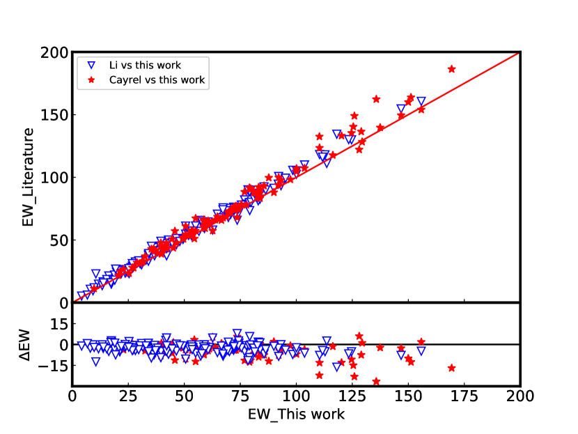
Figure 1: Comparison of the equivalent widths of HD2796, the blue circles represent the comparison of this work and Cayrel et al. (2004) ,while the black triangles represent the comparison of this this work and Li et al. (2015). Note that the biggest discrepancies between our EWs and the literature data are for the strongest lines. Thus, the spectrum synthesis approach have been used for these lines (e.g., Mg I tripletsg).

3 Stellar parameters

Despite the fact that iron abundances derived from both excitation levels (Fe I and Fe II) are affected by uncertainties in the model atmospheres temperature and NLTE effects (see Mashonkina et al., 2017, and reference therein), many researches still rely on this method (the so-called traditional spectroscopic method) to derive their stellar atmospheric parameters. Our adopted stellar parameters have been determined through this standard spectroscopic method. Additionally, we were able to determine effective temperatures from photometry and surface gravities from parallax/distances.

3.1 Effective temperature

The effective temperatures ($T_{\rm eff}$) were estimated by minimizing the trend between Fe I lines abundances and excitation potential ($\chi$).

To estimate $T_{\rm eff}$ from the available colors (B,V,J,H and K), we cross match our sample with two catalogs from the Virtual Observatory: The fourth US Naval Observatory CCD Astrograph Catalog (UCAC4, Zacharias et al. 2013 ) and Two Micron All Sky Survey (2MASS, Skrutskie et al. 2006) and then employ Ramírez & Meléndez (2005) temperature calibration. These $T_{\rm eff}$ (determined from photometric and spectroscopic methods) together with $T_{\rm eff}$  taken from Gaia DR2 (Gaia Collaboration et al., 2018) are in good agreement with each other ($\pm 150$ K).

3.2 Surface gravity and microturbulence

We determined the surface gravity $\log\,g$) by forcing Fe I abundances to agree with Fe II abundances. In addition, we crossed match our sample with Gaia DR2 distances catalogue (Bailer-Jones et al., 2018), to estimate the distance modulus from the available parallax of Gaia Collaboration et al. (2018) (see Eq. 2 and Eq. 3).

$$\log\frac{g}{g_{\odot}}=\log\frac{M}{M_{\odot}}+4\log\frac{T_{\rm eff}}{T_{\rm eff}}+0.4(M_{bol}-M_{bol_{\odot}})$$ (2)

$$M_{bol}=V+BC+5\log\varpi+5$$ (3)

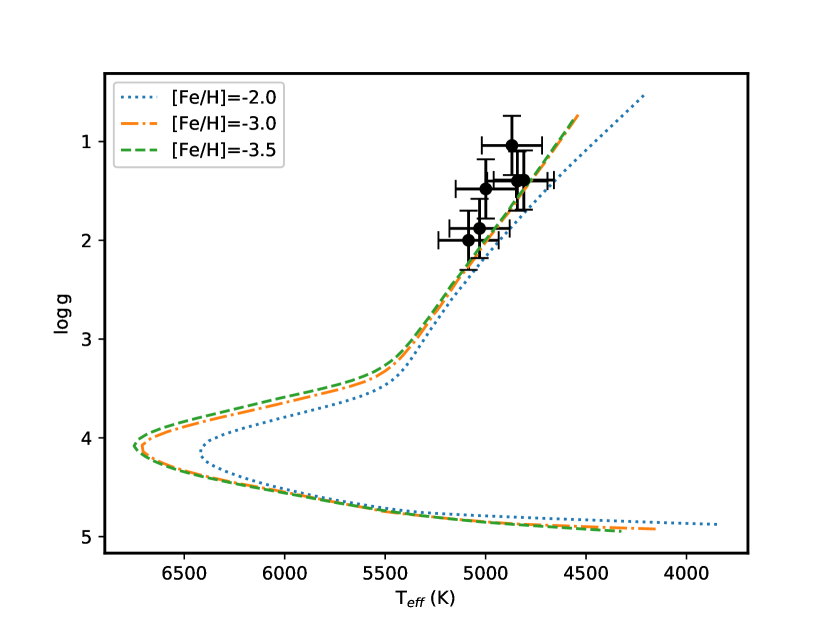
Figure 2: Our sample shown in an H-R-Diagram, based on the $T_{\rm eff}$ and $\log\,g$ determined from the LIKC/APF spectra (see Table 3). Yale-Yonsei 12 $\mathrm{Gyr}$  isochrones with [$\alpha$/Fe] = +0.4 and [Fe/H] = $-$2.5, $-$3.0, and $-$3.5 from Demarque et al. (2004) overplotted as reference.

where, $M$ is the stellar mass, $M_{bol}$ is the absolute bolometric magnitude, $V$ is the visual magnitude, $BC$ is the bolometric correction (see Alonso et al., 1999, Eq. 18), and $\pi$ is the parallax.

The microturbulence velocities ($\xi$) were determined by removing any trend between Fe I lines abundances with the EWs of those lines.

The $T_{\rm eff}$ determined from the photometric and spectroscopic methods show systematically different results. Frebel et al. (2013) have presented an explicit method to adjust the spectroscopic $T_{\rm eff}$. This scheme increases the $T_{\rm eff}$ determined for cool red-giants up-to several hundred degrees, on the other hand the $T_{\rm eff}$ determined for main-sequence stars are mostly unaffected. Motivated by Frebel et al. (2013) results, the atmospheric stellar parameters ($T_{\rm eff}$, $\log\,g$ and $\xi$) determined for our sample stars from the spectroscopic method were considered as initial parameters, and then corrected following the same scheme presented in Frebel et al. (2013). It’s worthy to note that our parameters were not determined independently. Thus, this procedure was iterated to consistency. The derived stellar atmospheric parameters are listed in Table 3.

The corrected spectroscopic surface gravities (in cgs units) versus the corrected spectroscopic $T_{\rm eff}$ of our programme stars, with 12 $\mathrm{Gyr}$ Yale-Yonsei isochrones as a reference (Demarque et al., 2004) are shown in Figure 2. The error bars shown in Figure 2 represent $T_{\rm eff}$  and $\log\,g$ one-sigma errors ($\pm 150$ K and $\pm 0.3$ cgs, respectively).

4 Abundance Analysis

We used only non-blended lines with reliable continuum normalization to measure the chemical abundances using EWs analysis. However, for the molecular bands and blended lines, spectral synthesis was used. In other words, our chemical abundances were done by a mixture of spectrum synthesis and equivalent width analysis. The LTE abundances for all elements are listed in Table 4. Moreover, we considered the deviations from LTE for Li I , Na I and Mg I lines. The LTE and NLTE abundances are presented in Table 5. We adopted the solar log$\epsilon_{\odot}$(X) from Asplund et al. (2009) to obtain our final chemical abundances and [X/Fe] ratios.

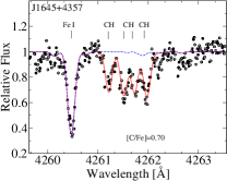
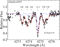
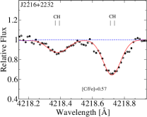
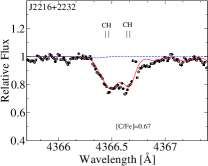
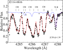
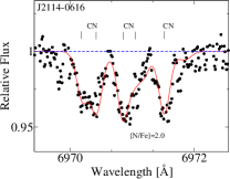
Figure 3: Portions of the LICK/APF spectra near the CH and CN bands (are represented as black filled circles). Best-fit of the selected CH and CN are also shown (red solid line). The dashed lines show the synthetic spectrum with no carbon in the atmosphere.

4.1 LTE and NLTE calculations

We used stellar atmosphere models from 1D ATLAS NEWODF grid of Castelli & Kurucz (2003). Our LTE abundances were performed using an updated version of the stellar code MOOG (Sneden, 1973). In this update, a continuous scattering will be treated as a source function, in other-words the absorption and scattering will be summed rather than treated as true absorption (Sobeck et al., 2011).

The departures from LTE in the stellar atmospheres were considered for three chemical elements, Li, Na, and Mg. The adopted Na I and Mg I-II model atoms are described in Alexeeva et al. (2014) and Alexeeva et al. (2018), respectively. To solve the radiative transfer and statistical equilibrium equations, we used the code detail (Butler & Giddings, 1985) based on the accelerated $\Lambda$-iteration method (Rybicki & Hummer, 1991). The obtained departure coefficients, $b_{\rm{i}}$ = $n_{\rm{NLTE}}$ / $n_{\rm{LTE}}$, were then used by the codes binmag3 (Kochukhov, 2010) and synthV-NLTE (Ryabchikova et al., 2016) to calculate the synthetic NLTE line profiles. Here, $n_{\rm{NLTE}}$ and $n_{\rm{LTE}}$ are the statistical equilibrium and thermal (Saha-Boltzmann) number densities, respectively.

We constructed the Li I model atom in the same manner as it was described in Lind et al. (2009). The main difference between our model atom and the model atom of Lind et al. (2009) is the collision excitation recipe. We adopted the electron collision data from Osorio et al. (2011), while Lind et al. (2009) used cross-sections for collisional excitation by electrons from Park (1971). We tested our model with Li-enhanced stars and have found a good agreement with Lind et al. (2009).

4.2 Lithium

Our LICK/APF spectra showed no obvious features for the lithium abundance determinations, except in J2216$+$2232 spectrum. Therefore, upper-limits were determined for the rest of the sample stars. The lithium abundance was derived from the Li I 6707.7 Å  resonance line. The line-list was taken from VALD database, hyperfine structure and isotope structure taken into account with the data from Sansonetti et al. (1995).

4.3 Carbon and Nitrogen

Our carbon abundances were derived from the molecular CH AX band around 4300 Å  The molecular line data for the spectrum synthesis was taken from VALD (Kupka et al., 1999) database. We determine carbon abundances using the method described in Alexeeva & Mashonkina (2015), our synthetic flux profiles were convolved with a profile that combines a rotational broadening and broadening by macroturbulence with a radial-tangential profile. The most probable macroturbulence velocity V_mac was varied between 4 and 9 km s^-1for different CH lines.

The nitrogen abundances were estimated from the CN 4215 Å  and 6971Å  bands, using a spectrum synthesis approach. The dissociation energy (D₀) of CN was adopted to be 7.65 eV (Bauschlicher et al., 1988). Only in J2114$-$0616 spectrum, we have found visible CN 4215 Å  and 6971Å  bands, which can be measured quite reliably. The best fits of some molecular lines in our sample are shown in Figure. 3.

4.4 Light Elements: from Na to Zn

We were able to measure abundances for Na, Mg, Ca, Ti, Sc, V, Cr, Mn, Co, Ni, and Zn in the LICK/APF spectra. Our sample stars are metal-poor and only resonance Na I lines at 5889, 5895 Å  are available for measurements. The van der Waals damping constant, C₆ = $-$31.6, for these lines was adopted from solar line-profile fitting (Zhao et al., 2016). The magnesium abundances are derived from Mg I lines at 4703, 5172, 5183, 5528, 5711 Å  (see Figure 4).

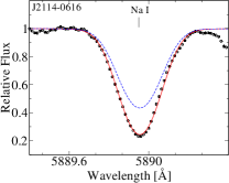
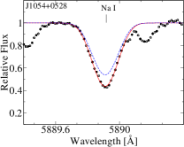
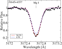
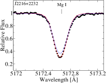
Figure 4: An example of the NLTE fittings of Na and Mg in LICK/APF spectra . The observed spectra are shown by filled circles, for comparison, the LTE profiles computed with the corresponding NLTE abundances are shown by the blue dashed curves.

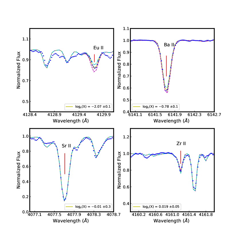
Figure 5: Portions of the LICK/APF spectrum of HD2796 (shown as blue filled circles) near the lines of Eu II at 4129 Å  (top left), Ba II at 6141 Å  (top right), Sr II at 4077 Å (bottom left), and Zr II at 4161 Å (bottom right). Best-fit synthetic spectra are also shown (yellow solid line), together with abundance variations (magenta dashed line and cyan dash-dotted line) of $\pm$0.1 dex (for Eu), $\pm$0.1 dex (for Ba), $\pm$0.3 dex (for Sr), and $\pm$0.5 dex (for Zr).

For the most of our sample stars, Ca abundances were derived from 18 well-defined Ca I lines, Ti abundances were obtained from 26 Ti I and Ti II lines in total, Scandium appeared in more than six Sc II lines, while V has only one reliable line at V I 4379.23 Å .

Cr I has at least 5 lines, while Mn I and Sc II lines appeared in all sample spectra. In our standard star HD2796 spectrum we were unable to find any detectable feature for Co I and Ni I, while they appeared in the remaining stars of our sample. Moreover, J1645$+$4357 spectrum shows no detectable line for the heaviest element of the iron peak Zn, see Table 4.

4.5 Neutron-capture Elements

The strontium (Sr) and barium (Ba) abundances for metal-poor stars are very important, since they are the most commonly detected neutron-capture elements whose abundances are measured in the vast majority of the metal-poor stars, thus these two elements are the key of understanding the nature of the neutron-capture processes in our Galaxy.

One of our main aims of the LICK/APF observations was to increase the high-resolution chemical inventory of metal-poor stars. In addition, to these elements mentioned previously, we also investigated yttrium, zirconium, lanthanum, cerium, praseodymium, neodymium, samarium, and europium, see Table 4.

Figure 5 shows an illustrative spectrum-synthesis example of the neutron-capture elements in our standard star HD2796. These elements show very weak features compared to those elements with Z$\leq 30$, with abundance uncertainties varying between 0.1 and 0.3 dex, depending on the quality of our spectrum-synthesis abundance measurements.

4.6 Uncertainties of stellar parameters and abundances

In Section 2.3 we discussed the uncertainties arising from the EWs. The stellar parameters are subject of another uncertainties arising from our ionization equilibrium process (the traditional spectroscopic method), where we expect that this process will provide typical internal accuracy in our estimated surface gravity and microturbulence of 0.1 dex and 0.2 km s^-1 respectively. In addition, these uncertainties will affect our abundances determination. The major uncertainties in our abundance determinations are related to the estimated effective temperatures (usually in the order of 100 K).

Figure 6: Abundances comparison between this work and Cayrel et al. (2004, for elements with Z$\leq 30$) and François et al. (2007, for neutron-capture elements). Excluding Sr abundance, the agreement is highly acceptable. The dashed line refers to $\Delta$= 0 and the dash-dotted lines refer to $\Delta=\pm 0.3$ dex.

Table 6 lists these abundance uncertainties for HD2796 (as an example), where we varied our atmospheric models effective temperature, surface gravity, and microturbulence by 150K, 0.3dex, and 0.3km s^-1 respectively. Figure 6 shows a comparison between our elemental abundances and Cayrel et al. (2004, for elements with Z$\leq 30$) and François et al. (2007, for neutron-capture elements). Apart from Sr (with $\Delta$ [Sr/Fe]=$-0.62$ relative to François et al.), the differences between our work and their work lie within $\pm 0.3$ dex (dash-dotted line in Figure 6). We impute our scattering to use cooler temperature, lower surface gravity, and lower S/N ratio than those used in Cayrel et al. (2004) and François et al. (2007) ($T_{\rm eff}$= 4950 K, $\log\,g$= 1.5 dex, and S/N ratio = 250-550).

5 Results and discussion

5.1 Chemical abundance comparison with literature data

We provided stellar parameters and detailed chemical abundances for five metal-poor red giant stars, reported for the first time using high resolution spectroscopy. These stars exhibit similar chemical abundance patterns to, reported in other, very and extremely metal-poor stars (e.g., François et al., 2007; Yong et al., 2013).

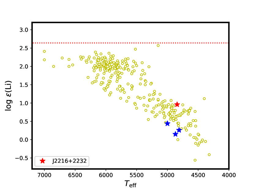
Figure 7: log$\epsilon$ lithium abundances as a function of effective temperature. Red filled star refers to J2216$+$2232, blue filled stars refer to the determined upper limits, and small open circles refer to the full sample of Roederer et al. (2014b). The dotted line shows the predicted primordial lithium abundance, log$\epsilon_{Li}$ = 2.64 (Spergel et al., 2007).

Lithium is considered as a key diagnostic, to test and constrain our understanding of the early Galaxy, of stellar interiors and evolution. Figure 7 illustrates the evolution of lithium as a function of $T_{\rm eff}$ using the halo star sample from Roederer et al. (2014b, including upper limits). The dotted line refers to the primordial lithium abundance predicted by the Standard Big Bang Nucleosynthesis (Spergel et al., 2007). Among the program stars, we could only detect Li in 2216$+$2232 (shown as red filled star) with A(Li) = 0.95. For completeness the upper limits for the rest of our sample stars have been provided (blue filled stars). This is not unexpected, as our sample stars are red-giants, whose Li content in the outer layers have been diluted by the canonical extra mixing and the first dredge-up (FDU) process.

Our sample stars exhibit relatively high [C/Fe] ratios, as shown in Figure 8 (left panel), which represents [C/Fe] ratio as a function of luminosity. We adopted a classification of Aoki et al. (2007), who suggest a scheme that takes into consideration the nucleosynthesis and mixing effects in giants. We define the stars that satisfy the following criteria as CEMP stars: [C/Fe]$\geqslant$0.7 for stars with $\log$(L/L_⊙)$\leqslant$2.3 and [C/Fe]$\geqslant$3.0$-$ $\log$(L/L_⊙) for stars with $\log$(L/L_⊙)$>$2.3. The luminosities of our stars were calculated based on the prescription of Aoki et al. (2007), assuming stellar mass of 0.8 M_⊙, following Aoki et al. (2005) and Ryan et al. (2005). For completeness, and due to the fact that our sample stars are gaints (see Figure 2), we use the carbon evolutionary correction described in Placco et al. (2014) to assess whether our sample stars could indeed be classified as CEMP, this method suggests that carbon levels decrease as stars evolve into the giant branch phase, due to some level of internal mixing. As a result, the correction increases the C abundances up to several dex, which support our claims that these stars are CEMP stars.

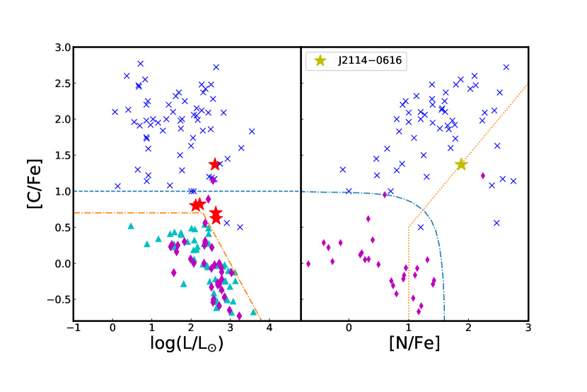
Figure 8: Left panel: [C/Fe] versus luminosity for our sample stars. The dash-dotted line indicates the dividing line between carbon-enhanced and carbon-normal stars as defined in Aoki et al. (2007). The dashed line corresponds to [C/Fe] = 1.0. Right panel: [C/Fe] vs. [N/Fe]. The two criteria for NEMP stars suggested by Pols et al. (2012) are respectively shown in dotted ([N/Fe] $\geq$ 1.0 and [N/C] $\geq$ 0.5) and dash-dotted lines ([(C+N)/Fe] $>$ 0.9). The filled red stars refer our sample stars. Non-carbon-enhanced objects studied by previous works (Gratton et al., 2000; Cayrel et al., 2004; Honda et al., 2004; Aoki et al., 2005) are shown by triangles up. Metal-poor stars from Spite et al. (2005) (filled diamonds), and CEMP stars from Aoki et al. (2007) (crosses) are also plotted for comparison. The candidate to CNEMP objects J2114-0616 is marked.

With the Aoki et al. (2007) definition of CEMP stars and the carbon evolutionary correction described in Placco et al. (2014) in mind, Figure 8 (left panel) shows that our program stars are located above the limit. Thus, we point J1054$+$0528, J1529$+$0804, J1645$+$4357, J2114$-$0616, and J2216$+$2232 as CEMP stars.

For most of our program stars CN bands are not measurable, we could only measure N abundance for J2114-0616, which exhibits high nitrogen abundance with [N/Fe]=1.88, [N/C]$>$0.51, and [(C+N)/Fe]=1.53. Figure 8 (right panel) shows [C/Fe] as a function of [N/Fe], with the dotted and dash-doted lines referring to Pols et al. (2012) NEMP stars criteria. We classify J2114$-$0616 as a potential nitrogen-enhanced metal-poor (NEMP) star. Since J2114$-$0616 satisfies both criteria (star with [C/Fe]$\geqslant$1.0 and [N/C]$\geqslant$0.5), it can be designated as a carbon and nitrogen-enhanced metal-poor (CNEMP) star.

Moreover, we investigated [Eu/Fe] as a function of [Ba/Fe] to study s-process and r-process enrichment, under the pretext that J2114$-$0616 shows 0.0$<$ [Ba/Eu] $<$ +0.5, and [Ba/Fe] $>$ 0.5 (see figure 9), we regard it as a CEMP-r/s star. In addition to the enhancements in both slow (s-) and rapid (r-) process species, J2114$-$0616 shows high [N/Fe] ratio, along with its high [C/Fe], which suggest that its peculiar chemical pattern may come from mass transfer from an AGB companion, before it tuned to a white dwarf.

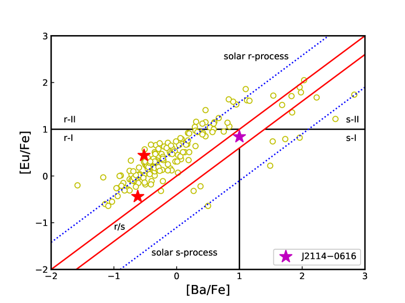
Figure 9: [Eu/Fe] as a function of [Ba/Fe], the open circles are data take from saga database (Suda et al., 2008) and the magenta star refer to the position of J2114$-$0616.

.

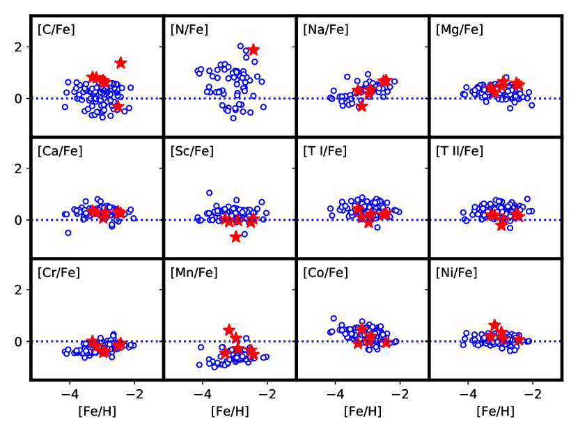
Figure 10: Comparison between the light-element abundances in our sample stars (red filled star) and the literature C-normal metal-poor stars from Yong et al. (2013) (blue open circles).

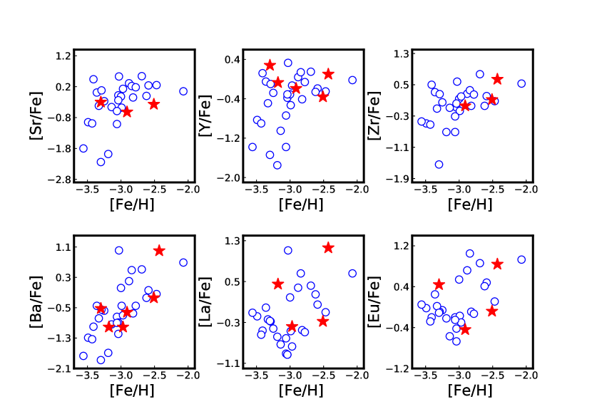
Figure 11: Selected neutron-capture elements abundances in our sample stars (red filled stars), as a function of metallicity, compared to literature data adopted from François et al. (2007) (blue open circles).

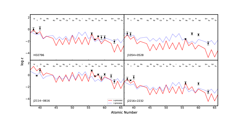
Figure 12: Abundance patterns for the neutron-capture elements in our sample. The solid line represents the Solar-system s-process abundance pattern from Burris et al. (2000), scaled to match the observed abundance of Ba in each star. The dotted line represents the Solar-system r-process abundance pattern from Burris et al. (2000), scaled to match the observed abundance of Eu in each star. Note that we only include these stars with measured Ba and Eu.

Light element distributions in CEMP stars are quite similar to those in non-carbon-enhanced stars (C-normal). The abundance ratios [X/Fe] as a function of [Fe/H] of our sample stars (red filled stars) are presented in Figure 10, for the elements from C through Zn, compared with literature data adopted from Yong et al. (2013) (blue open circles). In general, the abundance ratios seen in our sample show good agreement with the abundance ratio trends defined by the literature sample. On the other hand, J1529+0804, which shows enhancement in manganese with [Mn/Fe]=0.43, is not a good example of this agreement, this enhancement may also be true for J1645+4357 ([Mn/Fe]=0.12), keeping in mind that at low metallicities, the NLTE behavior may systematically increase the manganese abundance up to 0.7 dex (which we will explore in future work) (e.g., Bergemann & Gehren, 2008).

5.2 Nucleosynthetic signatures of s- and r-process

Only elements lighter than zinc can be produced via nuclear-fusions, on the other hand, heavier elements can be synthesized by either the rapid neutron capture process, r-process, and the slow neutron capture process, s-process (e.g., Meyer 1994; Arnould et al. 2007 and references therein). Metal-poor stars provide unique opportunities to attain nucleosynthetic signatures, thus better understanding of the chemical evolution of these elements and the nucleosynthesis occurred in the early Universe.

As mentioned previously, we were able to determine abundances for up to 10 heavy elements, including the light trans-iron elements ($38\leq$Z$\leq 46$) and the second r-process peak elements. The abundances of selected neutron-capture elements for our sample stars (red filled stars), as a function of the metallicity, overlaid with literature data adopted from François et al. (2007) (blue open circles) are shown in Figure 11. No significant discrepancies are found between the selected neutron-capture elements abundances of our sample stars and the literature data

Figure 12 shows the neutron-capture element abundances for HD2796 and three sample stars, compared with the Solar System s-process (normalized to Ba - solid line) and r-process (normalized to Eu - dotted line) components. The s- and r- fractions were taken from Burris et al. (2000). Abundances for the first-peak s-process elements (Sr, Y, and Zr) are well described by the Solar s-process for HD2796 and J2216+2232, while for J1054+0528 and J2114-0616 they are roughly consistent with the r-process component. At the same time, the noticeable deviations from for the light elements might interestingly be related to the effects of core-collapse supernovae. In contrast, for the second-peak s-process elements, there is an excellent agreement between measurements and the Solar s-process component for J2114-0616 which, combined with its enhancements in carbon and nitrogen, supports the hypothesis of mass transfer in a binary system from an AGB companion. For J1054+0528, it appears that all the neutron-capture element abundances are a result of an r-process event, with no contributions from the s-process component.

We could only detect weak Ba II lines in the spectrum of J1645$+$4357, which results in a relatively low Ba abundance while no other s-process elements can be detected. Such chemical patterns (high carbon, low barium, and absence of other s-process elements) suggests that J1645$+$4357 was formed out of pristine gas. The common definition of strongly r-process-enhanced star is [Eu/Fe] $>+1.0$ and [Ba/Eu] $<0$ and moderately r-process-enhanced star is (r-II stars) $+0.3\geq$[Eu/Fe]$\leq+1.0$ and [Ba/Eu] $<0$ (e.g., Frebel, 2018), adopting this criterion we suggest that J1054$+$0528 ([Eu/Fe]=0.44) is a new member of the moderately r-process-enhanced stars (r-I stars). On the other hand, J2114$-$0616 exhibits different chemical abundance patterns, enhancement of s-process species along with relatively high magnesium abundance suggesting that ²²Ne($\alpha$, n)²⁵Mg may have operate as a main neutron source in J2114$-$0616 (Masseron et al., 2010). Moreover, it turns out that the neutron density linked to this reaction favors the production of cerium (81% synthesized by s-process) and europium (97% synthesized by r-process), suggesting that these elements can’t be explained by s-process only, and additional r-process is required to describe this behavior (Gallino et al., 1998; Goriely & Mowlavi, 2000).

5.3 Kinematics and dynamics

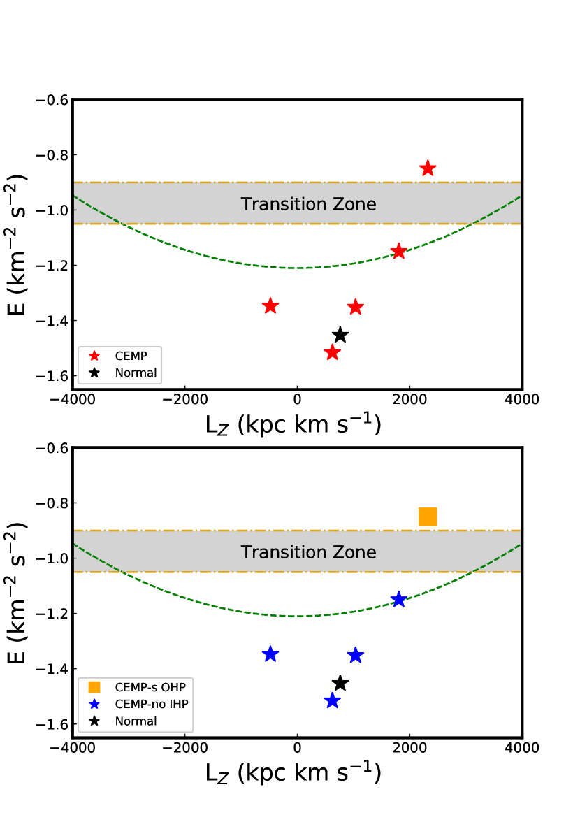
Figure 13: Total energy vs. angular momentum in the z direction for the stars in our sample. Top panel: C-normal stars are represented by black stars, while CEMP stars are denoted by red stars. Bottom panel: the same sample of stars, with blue filled star symbols indicating CEMP-no members of the inner halo, the orange filled square symbol represents the CEMP-no and CEMP-s members of the outer halo. The green dashed curve denotes the locus of the points that possess constant apo-Galactic radius, rapo = 15 kpc, while the golden dot-dashed horizontal lines shows the values of the energies delimiting the transition zone.

The full space motion is derived by combining the observables obtained by Gaia DR2, positions and proper motions ($\alpha$, $\delta$, $\mu_{\alpha}$, $\mu_{\delta}$). We utilize the software TOPCAT to cross match our sample with two catalogs from the Virtual Observatory: Gaia DR2 (Gaia Collaboration et al., 2018, for proper motions) and Gaia DR2 distances (Bailer-Jones et al., 2018, for distances), see Table 7. Radial velocities are obtained through cross-correlation with synthetic spectra after the heliocentric corrections to the observed spectra are applied. The velocities calculated in the Local Standard of Rest (LSR) are referred to as $(U,V,W)$ which are corrected for the motion of the Sun by adopting the values ($U,V,W$) = ($-$9,12,7) km s^-1 (Mihalas & Binney, 1981). The velocity component $U$ is taken to be positive in the direction towards the Galactic anti-centre, the $V$ component is positive in the direction towards Galactic rotation, and the $W$ component is positive toward the north Galactic pole. We also compute the rotational velocity component about the Galactic centre in a cylindrical frame, denoted as V_ϕ , and is calculated assuming that the LSR is on a circular orbit with a value of 220 km s^-1 (Kerr & Lynden-Bell, 1986). The orbital parameters are derived by adopting a Stäckel type gravitational potential (which consists of a flattened, oblate disk, and a nearly spherical massive dark-matter halo; a complete description is given by Chiba & Beers (2000, Appendix A) and integrating their orbital paths based on the starting point obtained from the observations.
In addition, we evaluate the integrals of motion for any given orbit, deriving the energy, E, and the angular momentum in the vertical direction, L_Z = R x V_ϕ. Note that R represents the distance from the Galactic center projected onto the disk plane. Typical errors on the orbital parameters (at Zmax $<$ 50 kpc; Carollo et al., 2010) are: $\sigma$_rperi $\sim$ 1 kpc, $\sigma$_rapo $\sim$ 2 kpc, $\sigma$_ecc $\sim$ 0.1, $\sigma$_Zmax $\sim$ 1 kpc.
Carollo et al. (2014) established a method for assigning the membership to the inner- and outer-halo stellar populations based on the integrals of motion (total energy and vertical angular momentum) of a large sample of SDSS/SEGUE DR7 calibration stars. Inner halo stars are mostly highly bound to the Galaxy (lower energy values, $E$ $<$ $-$1.1 km² s^-2) and possess orbits with apo-galactic distance r${}_{\rm apo}<$ 15 kpc, while outer halo stars are less bound to the Galaxy (higher energy values, $E$ $>$ $-$0.9 km² s^-2 ) and possess orbits with r${}_{\rm apo}>$ 15 kpc. Stars with r${}_{\rm apo}>$ 15 kpc and $E$ $<$ $-$1.1 km² s^-2 can be also considered pure inner halo stars. In general, stars in the outer halo are dominated by retrograde orbits but can also possess rotational velocities less retrograde or higlhy prograde, due to the large velocity dispersion of the outer halo ($\sim$ 165 km s^-1; Carollo et al., 2010). This is clearly evident in the right panel of Figure 4 in (Carollo et al., 2014) .
Figure 13 shows the total energy, E, as a function of the angular momentum in the vertical direction, L_Z, for the program stars. In the top panel, the black filled star symbol represents HD2796, while the red filled star symbols denote the CEMP stars. The grey horizontal area shows the range of binding energy values defining the transition zone between the inner- and the outer-halo components ($-$1.1 km² s^-2 $<E$ $<$ $-$0.9 km² s^-2), which is defined as the energy range where stars have similar probability to be members of these components. The green dashed curve represents the locus of stars possessing orbits with constant apo-galactic radius r_apo = 15 kpc. In the bottom panel the magenta star symbols denote the CEMP-no stars in the inner halo, classified according to their value of binding energy and apo-galactic distance, the CEMP-r/s star (J2114$-$0616) is represented by an orange filled square and it is member of the outer halo.
Figure 14 shows the galactocentric rotational velocity as a function of the metallicity for the program stars. It is interesting to note that J2114$-$0616 possesses a prograde motion (rotate in the same direction of the galactic disk) with velocities within $\sim$ 2$\sigma$ (CEMP-r/s; J2114$-$0616) of the mean rotational velocity of the outer halo population ($-$80 km s^-1). Highly prograde stars in the outer halo were also found in the sample of CEMP stars reported in Carollo et al. (2014, ; Figure 4).
Numerical cosmological simulations of MW-mass galaxies predict that stars in the inner halo of the MW formed mainly from massive subgalactic fragments that experienced an extended star formation activity (Zolotov et al., 2009; Font et al., 2011; McCarthy et al., 2012; Tissera et al., 2013, 2014), while outer halo stars formed predominantly in lower-mass subgalactic fragments with short or truncated star formation history (Carollo et al., 2007, 2010; Beers et al., 2012; Tissera et al., 2013, 2014; Carollo et al., 2016, 2018). The central regions of simulated halos (within $\sim$ 15 kpc) have an important contribution of in-situ stars (formed in the main progenitor galaxy) which have various possible origins (Brook et al., 2004; Zolotov et al., 2009; Font et al., 2011; House et al., 2011; Tissera et al., 2013; Cooper et al., 2015; Pillepich et al., 2015; Monachesi et al., 2016). On the contrary, stars in the outer halo formed primarily in low-mass subgalactic systems which were subsequently accreted. The origin of halo stars can be understood by inspecting a combination of their orbital parameters and integrals of motion. In case of our sample, J2114$-$0616, possesses orbital parameters, energy and vertical angular momentum that place it in the outer halo population and it likely were formed in low-mass systems outside the virial radius of the progenitor galaxy and accreted later on. The orbital parameters and binding energy of the remaining CEMP stars, J1054+0528, J1529+0804, J1645+4357 and J2216+2232, suggest that they are members of the inner halo population. However, their metallicity and C-enhancement indicate that they may have formed not in situ but in small mass subgalactic fragments which were accreted very early on and contributed to the old central regions of the halo system (Tissera et al., 2018; Carollo et al., 2018).

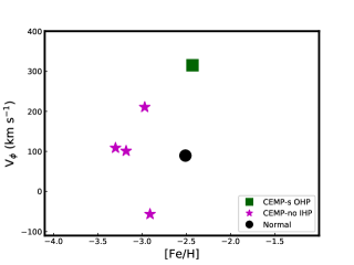
Figure 14: Galactocentric rotational velocity vs metallicity for the program stars color coded as in Figure 12.

6 conclusion

In this work we reported on the discovery of five CEMP stars selected from the LAMOST DR3 database as metal-poor candidates. High-resolution spectra are obtained for the first time with APF /LICK. We confirmed that J1054$+$0528, J1529$+$0804, J1645$+$4357, J2216$+$2232 and J2114$-$0616 show high enhancement in carbon with [C/Fe]= 0.82, 0.80, 0.70, 0.62, and 1.37, respectively, taking an advantage of their observed high-resolution spectra and the correction for evolutionary mixing. We provided stellar parameters and chemical abundances for up to 25 elements: three light elements (Li, C, N), 12 elements from Na to Zn, 10 neutron-capture elements (Sr, Y, Zr, Ba, La, Ce, Pr, Nd, Sm, and Eu). Our results show no significant abundance differences with literature, thus can be used to study the chemical enrichment at the earliest time of the Galaxy.

J1054+0528 shows moderate enhancement in europium [Eu/Fe]=0.44, with low barium-to-iron ratio [Ba/Fe]=$-$0.52. These abundances indicate that this star can be classified as CEMP-rI and future higher signal-to-noise observations should be carried out to obtain abundances of other r-process elements, such as Gd, Th, Os, Pt, and Pb.

No reliable s-process elements lines were found in J1645$+$4357 spectrum. More accurate measurements of more heavy elements would be needed for further deduction. Thus, we strongly recommend future observation of J1645$+$4357 in the near-ultraviolet spectroscopy, to determine many key elements such as Ge, Zr, Os, Pt, and Pb.

J2114$-$0616 can be classified as CNEMP-r/s (carbon nitrogen-enhanced metal-poor) star, due to the high enhancement in nitrogen with [N/Fe]= 1.88, [N/C]= 0.5, barium [Ba/Fe]=1.00, and europium [Eu/Fe]=0.84. Other r-process elements, such as Gd, Th, Os, Pt, and Pb can be obtained in future high resolution and high signal-to-noise observations.

Kinematic and dynamic analysis based on Gaia DR2 parameters reveals that J2114$-$0616 is stellar members of the outer halo population and suggests that it may have formed in low-mass systems outside the virial radius of the progenitor galaxy and accreted later on during the merging and disruption of such systems. The stars J1054+0528, J1529+0804, J1645+4357 and J2216+2232 are stellar members of the inner halo population, however their very low metallicity and enhancement in carbon abundance strongly indicate that they were born in low-mass sub-galactic systems which were accreted during the initial phases of Galaxy assembly and contributed to the old stellar populations of the inner halo.

Table 1: Log of the Lick/APF observations.

	ID	Date	RA	DEC	$r$	Exptime	S/N	$V_{r}$
					(mag)	(s)	(pixel${}^{-1})$	(km s-1)
1	HD2796	18 Nov 2015	00 31 16.91	$-$16 47 40.8	8.51	900*2	43	$-$60.51
2	J1054$+$0528	28 May 2015	10 54 33.10	$+$05 28 12.7	12.65	1800*4	42	82.36
3	J1529$+$0804	30 May 2015	15 29 53.94	$+$08 04 48.1	12.49	1800*4	46	23.40
4	J1645$+$4357	28 May 2015	16 45 14.95	$+$43 57 12.0	12.79	1800*4	40	$-$83.20
5	J2114$-$0616	23 Sep 2015	21 14 01.52	$-$06 16 10.3	10.81	1200*4	46	$-$160.32
6	J2216$+$2232	27 July 2015	22 16 39.31	$+$22 32 50.4	12.03	1800*4	47	$-$339.38

Note. — The S/N ratio per pixel was measured at $\lambda\sim 4500$ Å .

Luminosity was derived based on Aoki et al. (2007) relation

Table 2: Equivalent widths of our sample.

$\lambda$	Species	$\chi$	$\log\,gf$	HD2796	J1054+0528	J1529+0804	J1645+4357	2114$-$0616	J2216+2232
(Å )		eV		mÅ	mÅ	mÅ	mÅ	mÅ	mÅ
4049	C(CH)	—	—	—	syn	—	—	syn	—
4218	C(CH)	—	—	syn	syn	—	—	syn	syn
4248	C(CH)	—	—	—	—	syn	syn	syn	—
4253	C(CH)	—	—	syn	—	syn	—	syn	syn
4261	C(CH)	—	—	—	—	—	syn	—	—
4273	C(CH)	—	—	—	syn	—	syn	syn	syn
4279	C(CH)	—	—	—	—	—	syn	syn	syn
4281	C(CH)	—	—	syn	—	—	—	syn	syn
4292	C(CH)	—	—	—	syn	syn	—	syn	—
4310	C(CH)	—	—	—	—	syn	—	—	syn
4313	C(CH)	—	—	syn	—	—	syn	syn	—
4362	C(CH)	—	—	—	syn	—	—	—	syn
4366	C(CH)	—	—	—	—	—	syn	—	syn
4214	N(CN)	—	—	—	—	—	—	syn	—
6970	N(CN)	—	—	—	—	—	—	syn	—
5889.95	Na I	0.00	0.10	169.6	118.7	66.4	174.2	195.0	140.0
5895.92	Na I	0.00	-0.20	164.8	120.4	65.1	161.1	181.8	159.4
4702.99	Mg I	4.33	-0.44	77.2	26.1	8.8	64.5	73.0	51.3
5172.68	Mg I	2.71	-0.45	217.9	124.4	209.7	211.0	183.6
5183.60	Mg I	2.72	-0.24	260.2	145.6	147.8	232.1	267.0	218.5
5528.40	Mg I	4.35	-0.50	68.7	36.2	33.7	72.7	81.3	48.0
5711.09	Mg I	4.35	-1.72	3.5	10.5	—	—	9.7	5.3
4283.01	Ca I	1.89	-0.22	60.9	—	15.2	54.9	78.5	59.9
4318.65	Ca I	1.89	-0.21	64.7	—	—	—	22.2	40.0
4425.44	Ca I	1.88	-0.36	50.9	27.2	19.3	—	52.9	—
4454.78	Ca I	1.90	0.26	81.9	31.9	46.5	42.1	76.4	64.9
4455.89	Ca I	1.90	-0.53	43.9	—	18.8	—	38.7	15.9

Note. — Table 2 is published in its entirety in the machine-readable format. A portion is shown here for guidance regarding its form and content.

Table 3: Stellar Parameters of the Program Stars.

	Lick/APF (adopted)				LAMOST					Gaia DR2					Photometry				Luminosity
ID	$T_{\rm eff}$	$\log\,g$	[Fe/H]	$\xi$		$T_{\rm eff}$	$\log\,g$	[Fe/H]			$T_{\rm eff}$	$\log\,g$				$T_{\rm eff}$			$~{}~{}L_{\ast}/L_{\odot}$
	(K)	(cgs)		(kms-1)		(K)	(cgs)				(K)	(cgs)				(K)			(ergs-1)
HD2796	4869	1.04	$-$2.51	2.01		…	…	…			4995	2.15				…			1014.0
J1054$+$0528	5030	1.88	$-$3.30	1.94		5094	1.76	$-$3.23			5080	1.89				4981			166.94
J1529$+$0804	5085	2.00	$-$3.18	2.34		5026	1.54	$-$3.27			5041	1.90				4913			132.27
J1645$+$4357	4810	1.39	$-$2.97	2.93		4715	2.14	$-$3.05			4886	1.39				4652			431.38
J2114$-$0616	4999	1.48	$-$2.43	2.11		4377	1.55	$-$2.95			4870	1.66				4831			409.09
J2216$+$2232	4842	1.40	$-$2.91	1.79		4902	2.65	$-$3.13			5018	2.05				4815			432.89

Note. — The tenth column was measured using parallaxes adopted from Gaia DR2 and stellar mass of $\sim$ 0.8 M_⊙

Table 4: LTE Abundances of Individual Elements for the Program Stars.

	HD2796					J1054$+$0528					J1529$+$0804
	log $\epsilon$(X)	[X/Fe]	$\sigma$	$N$		log $\epsilon$(X)	[X/Fe]	$\sigma$	$N$		log $\epsilon$(X)	[X/Fe]	$\sigma$	$N$
Li I	…	…	…	…		…	…	…	…		…	…	…	…
C(CH)	5.60	$-$0.31	0.05	5		5.95	0.82	0.09	6		6.05	0.80	0.11	4
(CH)corr	…	0.74	…	…		…	0.04	…	…		…	0.01	…	…
N(CN)	…	…	…	…		…	…	…	…		…	…	…	…
Na I	4.40	0.67	0.05	2		3.25	0.31	0.05	2		2.76	$-$0.30	0.24	2
Mg I	5.68	0.59	0.05	4		4.71	0.41	0.12	5		4.64	0.22	0.10	4
Ca I	4.15	0.32	0.10	21		3.39	0.35	0.29	11		3.46	0.30	0.18	17
Sc II	0.55	$-$0.09	0.05	13		$-$0.12	0.03	0.24	6		$-$0.10	$-$0.07	0.05	3
Ti I	2.64	0.20	0.09	18		2.08	0.43	0.25	13		1.87	0.10	0.30	11
Ti II	2.67	0.23	0.12	33		1.84	0.19	0.30	25		1.95	0.18	0.32	24
V I	1.36	$-$0.06	0.11	1		0.93	0.30	0.13	1		…	…	…	…
Cr I	2.97	$-$0.16	0.10	9		2.34	0.00	0.30	5		2.27	$-$0.19	0.29	8
Mn I	2.57	$-$0.35	0.12	3		1.67	$-$0.46	0.10	1		2.68	0.43	0.02	2
Fe I	4.99	0.00	0.12	217		4.20	0.00	0.16	84		4.32	0.00	0.26	146
Fe II	4.99	0.00	0.09	24		4.20	0.00	0.18	8		4.32	0.00	0.25	17
Co I	…	…	…	…		1.61	$-$0.08	0.20	2		2.29	0.48	0.06	3
Ni I	…	…	…	…		3.10	0.18	0.13	4		3.66	0.62	0.32	7
Zn I	2.33	0.28	0.03	2		…	…	…	…		1.95	0.57	0.12	1
Sr II	$-$0.01	$-$0.37	0.10	1		$-$0.73	$-$0.30	0.13	1		…	…	…	…
Y II	$-$0.66	$-$0.36	0.06	3		$-$0.81	0.28	0.16	1		$-$1.04	$-$0.07	0.19	2
Zr II	0.19	0.12	0.12	1		…	…	…	…		…	…	…	…
Ba II	$-$0.57	$-$0.24	0.22	3		$-$1.64	$-$0.52	0.10	3		$-$2.01	$-$1.01	0.13	2
La II	$-$1.69	$-$0.28	0.04	2		…	…	…	…		$-$1.63	0.45	0.13	1
Ce II	$-$1.18	$-$0.25	0.10	3		$-$0.74	0.98	0.20	2		$-$0.77	0.84	0.11	2
Pr II	$-$1.36	0.43	0.17	1		…	…	…	…		$-$0.88	1.58	0.19	1
Nd II	$-$1.34	$-$0.25	0.26	7		$-$0.91	0.97	0.19	9		$-$0.71	1.05	0.58	5
Sm II	…	…	…	…		…	…	…	…		$-$0.60	1.62	0.05	2
Eu II	$-$2.07	$-$0.08	0.11	1		$-$2.34	0.44	0.14	1		…	…	…	…

Table 4: Continued.

	J1645$+$4357					J2114$-$0616					J2216$+$2232					Sun
	log $\epsilon$(X)	[X/Fe]	$\sigma$	$N$		log $\epsilon$(X)	[X/Fe]	$\sigma$	$N$		log $\epsilon$(X)	[X/Fe]	$\sigma$	$N$			log $\epsilon$(X)
Li I	…	…	…	…		…	…	…	…		0.96	2.82	0.04	1			1.05
C(CH)	6.16	0.70	0.04	6		7.37	1.37	0.05	10		6.14	0.62	0.05	8			8.43
(CH)corr	…	0.45	…	…		…	0.17	…	…		…	0.45	…	…			…
N(CN)	…	…	…	…		7.28	1.88	0.17	2		…	…	…	…			7.83
Na I	3.45	0.18	0.04	2		4.69	0.88	0.05	2		3.68	0.35	0.05	2			6.24
Mg I	5.12	0.49	0.05	4		5.69	0.52	0.12	5		5.34	0.65	0.02	4			7.60
Ca I	3.44	0.07	0.28	11		4.17	0.26	0.29	20		3.70	0.27	0.17	18			6.34
Sc II	$-$0.48	$-$0.66	0.23	4		0.75	0.04	0.25	13		0.22	$-$0.02	0.14	8			3.15
Ti I	1.88	$-$0.10	0.26	11		2.78	0.26	0.16	15		2.26	0.22	0.13	15			4.95
Ti II	1.76	$-$0.21	0.25	25		2.65	0.13	0.31	30		2.05	0.01	0.27	26			4.95
V I	…	…	…	…		…	…	…	…		…	…	…	…			3.93
Cr I	2.24	$-$0.43	0.30	6		3.13	$-$0.08	0.09	8		2.35	$-$0.38	0.22	10			5.64
Mn I	2.58	0.12	0.08	2		2.49	$-$0.51	0.03	2		2.24	$-$0.28	0.21	2			5.43
Fe I	4.53	0.00	0.22	150		5.07	0.00	0.14	156		4.58	0.00	0.18	181			7.50
Fe II	4.53	0.00	0.20	18		5.07	0.00	0.17	24		4.58	0.00	0.19	20			7.50
Co I	2.04	0.02	0.09	1		2.51	$-$0.05	0.03	2		2.27	0.19	0.11	3			4.99
Ni I	3.60	0.35	0.16	8		3.85	0.06	0.10	11		3.40	0.09	0.15	9			6.22
Zn I	…	…	…	…		2.43	0.30	0.12	2		1.92	0.27	0.04	2			4.56
Sr II	…	…	…	…		…	…	…	…		$-$0.66	$-$0.62	0.08	1			2.87
Y II	…	…	…	…		$-$0.12	0.10	0.03	2		$-$0.89	$-$0.19	0.09	2			2.21
Zr II	…	…	…	…		0.79	0.64	0.13	1		$-$0.37	$-$0.04	0.10	1			2.58
Ba II	$-$1.80	$-$1.01	0.15	3		0.75	1.00	0.11	3		$-$1.35	$-$0.62	0.25	3			2.18
La II	$-$2.25	$-$0.38	0.11	1		$-$0.17	1.16	0.02	2		…	…	…	…			1.10
Ce II	…	…	…	…		0.08	0.93	0.12	3		…	…	…	…			1.58
Pr II	…	…	…	…		$-$0.49	1.22	0.15	1		…	…	…	…			0.72
Nd II	…	…	…	…		0.10	1.11	0.17	8		$-$1.46	0.03	0.22	5			1.42
Sm II	…	…	…	…		$-$0.18	1.29	0.12	1		…	…	…	…			0.96
Eu II	…	…	…	…		$-$1.07	0.84	0.13	1		$-$2.84	$-$0.44	0.12	1			1.07

Note. — N refers to the number of lines adopted for determination of the elemental abundances.

Table 5: Li, Na, Mg NLTE abundances

Star	log$\epsilon$(Li)		log$\epsilon$(Na)		[Na/Fe]NLTE	log$\epsilon$(Mg)		[Mg/Fe]NLTE
	LTE	NLTE	LTE	NLTE		LTE	NLTE
HD2796	$<$ 0.14	$<$ 0.15	4.40	3.65	$-$0.08	5.68	5.69	0.60
J1054$+$0528	…	…	3.25	2.91	$-$0.03	4.71	4.81	0.51
J1529$+$0804	$<$ 0.30	$<$ 0.32	2.76	2.53	$-$0.53	4.64	4.75	0.33
J1645$+$4357	$<$ 0.24	$<$ 0.26	3.45	2.97	$-$0.30	5.12	5.10	0.47
J2114$-$0616	$<$ 0.44	$<$ 0.44	4.69	3.88	0.07	5.69	5.69	0.52
J2216$+$2232	0.95	0.96	3.68	3.06	$-$0.27	5.34	5.33	0.64

Note. — J1054$+$0528 has defect in the spectrum at the region of the Li I line.

Table 6: Uncertainties of log $\epsilon$(X) Propagated from the Stellar Parameters (as Described in Section 4.6), Computed for HD2796 as an Example.

Ion	$\Delta$Teff	$\Delta$$\log\,g$	$\Delta\xi$
	$+$ 150 K	$+$ 0.3 dex	$+$ 0.3 km s-1
CH(C)	0.32	$-$0.12	0.02
CN(N)	0.50	$-$0.10	0.01
Na I	0.16	$-$0.05	$-$0.03
Mg I	0.14	$-$0.11	$-$0.03
Ca I	0.05	$-$0.02	$-$0.11
Sc II	0.09	$-$0.12	$-$0.13
Ti I	$-$0.03	0.00	$-$0.02
Ti II	0.11	-0.12	-0.13
V II	$-$0.04	0.00	$-$0.02
Cr II	$-$0.02	$-$0.01	$-$0.01
Mn I	0.01	$-$0.01	$-$0.08
Fe I	0.16	$-$0.03	$-$0.15
Fe II	0.15	$-$0.13	$-$0.219
Co I	$-$0.04	0.01	0.03
Ni I	$-$0.01	$-$0.05	$-$0.13
Zn I	0.06	$-$0.06	$-$0.18
Sr II	0.06	$-$0.07	0.08
Y II	0.07	$-$0.13	$-$0.17
Zr I	0.07	$-$0.12	$-$0.16
Ba II	0.02	$-$0.12	0.08
La II	0.04	$-$0.12	$-$0.14
Ce II	0.05	$-$0.12	$-$0.15
Pr II	0.03	$-$0.12	$-$0.13
Nd II	0.03	$-$0.12	$-$0.13
Eu II	0.05	$-$0.12	$-$0.14

Table 7: Parallaxes, Proper Motions and Distances

Star	Gaia DR2 source ID	$\varpi$	error		pmra	error		pmdec	error		Distance	d1	d2
		(mas)			(mas yr-1)			(mas yr-1)			(kpc)
HD2796	2367454697327877504	1.4859	0.0626		$-$1.375	0.164		$-$51.052	0.084		0.661	0.027	0.028
J1054$+$0528	3864140775805950208	0.2149	0.0393		$-$8.678	0.073		$-$ 4.183	0.055		3.548	0.404	0.502
J1529$+$0804	1164484488577137792	0.2365	0.0362		$-$2.401	0.056		$-$9.169	0.05		3.628	0.425	0.544
J1645$+$4357	1357725650023190784	0.0454	0.0207		0.327	0.033		$-$5.663	0.042		8.355	0.996	1.215
J2114$-$0616	6910940758263238912	0.4496	0.0373		$-$20.444	0.067		$-$6.376	0.068		2.082	0.153	0.178
J2216$+$2232	1878089211702170880	0.3721	0.0384		$-$4.454	0.056		$-$1.477	0.058		2.440	0.211	0.253

Note. — The d1 and d2 columns indicate the 16th percentile and 84th percentile confidence intervals.

Table 8: Kinematics parameters

Star ID	VR	VΦ	VZ	V⟂	Zmax	Rapo	Rperi	e	E	Lz
HD2796	-95.03	89.62	37.81	102.28	1.02	9.59	2.28	0.62	-1.45	763.40
J1054$+$0528	82.98	108.74	-15.88	84.49	3.59	10.81	3.60	0.50	-1.35	1036.00
J1529$+$0804	-86.75	101.22	-8.18	87.13	3.01	7.43	2.52	0.50	-1.52	624.00
J1645$+$4357	-74.40	210.51	-58.18	94.45	7.67	14.50	7.82	0.30	-1.15	1807.00
J2114$-$0616	-220.45	314.95	37.41	223.60	4.70	33.16	5.64	0.71	-0.85	2323.00
J2216$+$2232	-35.03	-56.42	182.30	185.64	8.70	9.22	4.08	0.41	-1.35	-478.40

References

- Abate et al. (2015) Abate, C., Pols, O. R., Izzard, R. G., & Karakas, A. I. 2015, A&A, 581, A22
- Abbott et al. (2017) Abbott, B. P., Abbott, R., Abbott, T. D., et al. 2017, Physical Review Letters, 119, 161101
- Alexeeva et al. (2018) Alexeeva, S., Ryabchikova, T., Mashonkina, L., & Hu, S. 2018, ArXiv e-prints, arXiv:1809.06969
- Alexeeva & Mashonkina (2015) Alexeeva, S. A., & Mashonkina, L. I. 2015, MNRAS, 453, 1619
- Alexeeva et al. (2014) Alexeeva, S. A., Pakhomov, Y. V., & Mashonkina, L. I. 2014, Astronomy Letters, 40, 406
- Alonso et al. (1999) Alonso, A., Arribas, S., & Martínez-Roger, C. 1999, A&AS, 140, 261
- Aoki et al. (2007) Aoki, W., Beers, T. C., Christlieb, N., et al. 2007, ApJ, 655, 492
- Aoki et al. (2005) Aoki, W., Honda, S., Beers, T. C., et al. 2005, ApJ, 632, 611
- Aoki et al. (2013) Aoki, W., Beers, T. C., Lee, Y. S., et al. 2013, AJ, 145, 13
- Arnould et al. (2007) Arnould, M., Goriely, S., & Takahashi, K. 2007, Phys. Rep., 450, 97
- Asplund et al. (2009) Asplund, M., Grevesse, N., Sauval, A. J., & Scott, P. 2009, ARA&A, 47, 481
- Astropy Collaboration et al. (2013) Astropy Collaboration, Robitaille, T. P., Tollerud, E. J., et al. 2013, A&A, 558, A33
- Astropy Collaboration et al. (2018) Astropy Collaboration, Price-Whelan, A. M., Sipőcz, B. M., et al. 2018, AJ, 156, 123
- Bailer-Jones et al. (2018) Bailer-Jones, C. A. L., Rybizki, J., Fouesneau, M., Mantelet, G., & Andrae, R. 2018, AJ, 156, 58
- Bauschlicher et al. (1988) Bauschlicher, Jr., C. W., Langhoff, S. R., & Taylor, P. R. 1988, ApJ, 332, 531
- Beers et al. (2012) Beers, T. C., Carollo, D., Lee, Y., Kennedy, C. R., & SEGUE Collaboration. 2012, in American Astronomical Society Meeting Abstracts, Vol. 219, American Astronomical Society Meeting Abstracts #219, 222.06
- Beers & Christlieb (2005) Beers, T. C., & Christlieb, N. 2005, ARA&A, 43, 531
- Bergemann & Gehren (2008) Bergemann, M., & Gehren, T. 2008, A&A, 492, 823
- Bessell & Norris (1982) Bessell, M. S., & Norris, J. 1982, ApJ, 263, L29
- Brook et al. (2004) Brook, C. B., Kawata, D., Gibson, B. K., & Freeman, K. C. 2004, ApJ, 612, 894
- Burbidge et al. (1957) Burbidge, E. M., Burbidge, G. R., Fowler, W. A., & Hoyle, F. 1957, Reviews of Modern Physics, 29, 547
- Burris et al. (2000) Burris, D. L., Pilachowski, C. A., Armandroff, T. E., et al. 2000, ApJ, 544, 302
- Butler & Giddings (1985) Butler, K., & Giddings, J. 1985, Newsletter on the analysis of astronomical spectra, No. 9, University of London
- Caffau et al. (2018) Caffau, E., Gallagher, A. J., Bonifacio, P., et al. 2018, A&A, 614, A68
- Caffau et al. (2011) Caffau, E., Bonifacio, P., François, P., et al. 2011, Nature, 477, 67
- Carollo et al. (2014) Carollo, D., Freeman, K., Beers, T. C., et al. 2014, ApJ, 788, 180
- Carollo et al. (2018) Carollo, D., Tissera, P. B., Beers, T. C., et al. 2018, ApJ, 859, L7
- Carollo et al. (2007) Carollo, D., Beers, T. C., Lee, Y. S., et al. 2007, Nature, 450, 1020
- Carollo et al. (2010) Carollo, D., Beers, T. C., Chiba, M., et al. 2010, ApJ, 712, 692
- Carollo et al. (2012) Carollo, D., Beers, T. C., Bovy, J., et al. 2012, ApJ, 744, 195
- Carollo et al. (2016) Carollo, D., Beers, T. C., Placco, V. M., et al. 2016, Nature Physics, 12, 1170
- Castelli & Kurucz (2003) Castelli, F., & Kurucz, R. L. 2003, in IAU Symposium, Vol. 210, Modelling of Stellar Atmospheres, ed. N. Piskunov, W. W. Weiss, & D. F. Gray, A20
- Cayrel (1988) Cayrel, R. 1988, in IAU Symposium, Vol. 132, The Impact of Very High S/N Spectroscopy on Stellar Physics, ed. G. Cayrel de Strobel & M. Spite, 345
- Cayrel et al. (2004) Cayrel, R., Depagne, E., Spite, M., et al. 2004, A&A, 416, 1117
- Chiaki et al. (2017) Chiaki, G., Susa, H., & Hirano, S. 2017, Mem. Soc. Astron. Italiana, 88, 856
- Chiappini et al. (2005) Chiappini, C., Matteucci, F., & Ballero, S. K. 2005, A&A, 437, 429
- Chiba & Beers (2000) Chiba, M., & Beers, T. C. 2000, AJ, 119, 2843
- Christlieb et al. (2002) Christlieb, N., Bessell, M. S., Beers, T. C., et al. 2002, Nature, 419, 904
- Cooper et al. (2015) Cooper, A. P., Parry, O. H., Lowing, B., Cole, S., & Frenk, C. 2015, MNRAS, 454, 3185
- Cruz et al. (2018) Cruz, M. A., Cogo-Moreira, H., & Rossi, S. 2018, MNRAS, 475, 4781
- Cui et al. (2012) Cui, X.-Q., Zhao, Y.-H., Chu, Y.-Q., et al. 2012, Research in Astronomy and Astrophysics, 12, 1197
- Demarque et al. (2004) Demarque, P., Woo, J.-H., Kim, Y.-C., & Yi, S. K. 2004, ApJS, 155, 667
- Ekström et al. (2008) Ekström, S., Meynet, G., Chiappini, C., Hirschi, R., & Maeder, A. 2008, A&A, 489, 685
- Font et al. (2011) Font, A. S., McCarthy, I. G., Crain, R. A., et al. 2011, MNRAS, 416, 2802
- François et al. (2007) François, P., Depagne, E., Hill, V., et al. 2007, A&A, 476, 935
- Frebel (2018) Frebel, A. 2018, Annual Review of Nuclear and Particle Science, 68, 237
- Frebel et al. (2013) Frebel, A., Casey, A. R., Jacobson, H. R., & Yu, Q. 2013, ApJ, 769, 57
- Frebel & Norris (2015) Frebel, A., & Norris, J. E. 2015, ARA&A, 53, 631
- Frebel et al. (2005) Frebel, A., Aoki, W., Christlieb, N., et al. 2005, Nature, 434, 871
- Gaia Collaboration et al. (2018) Gaia Collaboration, Brown, A. G. A., Vallenari, A., et al. 2018, A&A, 616, A1
- Gallino et al. (1998) Gallino, R., Arlandini, C., Busso, M., et al. 1998, ApJ, 497, 388
- Goriely & Mowlavi (2000) Goriely, S., & Mowlavi, N. 2000, A&A, 362, 599
- Gratton et al. (2000) Gratton, R. G., Sneden, C., Carretta, E., & Bragaglia, A. 2000, A&A, 354, 169
- Grillmair (2009) Grillmair, C. J. 2009, ApJ, 693, 1118
- Hansen et al. (2016a) Hansen, C. J., Nordström, B., Hansen, T. T., et al. 2016a, A&A, 588, A37
- Hansen et al. (2016b) Hansen, T. T., Andersen, J., Nordström, B., et al. 2016b, A&A, 588, A3
- Helmi et al. (2018) Helmi, A., Babusiaux, C., Koppelman, H. H., et al. 2018, Nature, 563, 85
- Hirano et al. (2014) Hirano, S., Hosokawa, T., Yoshida, N., et al. 2014, ApJ, 781, 60
- Hirschi (2007) Hirschi, R. 2007, A&A, 461, 571
- Honda et al. (2004) Honda, S., Aoki, W., Kajino, T., et al. 2004, ApJ, 607, 474
- House et al. (2011) House, E. L., Brook, C. B., Gibson, B. K., et al. 2011, MNRAS, 415, 2652
- Hunter (2007) Hunter, J. D. 2007, Computing In Science & Engineering, 9, 90
- Ito et al. (2013) Ito, H., Aoki, W., Beers, T. C., et al. 2013, ApJ, 773, 33
- Izzard et al. (2009) Izzard, R. G., Glebbeek, E., Stancliffe, R. J., & Pols, O. R. 2009, A&A, 508, 1359
- Jeon et al. (2017) Jeon, M., Besla, G., & Bromm, V. 2017, ApJ, 848, 85
- Ji et al. (2016) Ji, A. P., Frebel, A., Chiti, A., & Simon, J. D. 2016, Nature, 531, 610
- Joggerst et al. (2010) Joggerst, C. C., Almgren, A., Bell, J., et al. 2010, ApJ, 709, 11
- Johnson et al. (2007) Johnson, J. A., Herwig, F., Beers, T. C., & Christlieb, N. 2007, ApJ, 658, 1203
- Jones et al. (2001–) Jones, E., Oliphant, T., Peterson, P., et al. 2001–, SciPy: Open source scientific tools for Python, , , [Online; accessed ¡today¿]
- Keller et al. (2014) Keller, S. C., Bessell, M. S., Frebel, A., et al. 2014, Nature, 506, 463
- Kerr & Lynden-Bell (1986) Kerr, F. J., & Lynden-Bell, D. 1986, MNRAS, 221, 1023
- Kielty et al. (2017) Kielty, C. L., Venn, K. A., Loewen, N. B., et al. 2017, MNRAS, 471, 404
- Kochukhov (2010) Kochukhov, O. 2010, ,
- Kupka et al. (1999) Kupka, F., Piskunov, N., Ryabchikova, T. A., Stempels, H. C., & Weiss, W. W. 1999, A&AS, 138, 119, (VALD)
- Li et al. (2015) Li, H.-N., Zhao, G., Christlieb, N., et al. 2015, ApJ, 798, 110
- Lind et al. (2009) Lind, K., Asplund, M., & Barklem, P. S. 2009, A&A, 503, 541
- Lucatello et al. (2005) Lucatello, S., Tsangarides, S., Beers, T. C., et al. 2005, ApJ, 625, 825
- Mashonkina et al. (2017) Mashonkina, L., Jablonka, P., Pakhomov, Y., Sitnova, T., & North, P. 2017, A&A, 604, A129
- Masseron et al. (2010) Masseron, T., Johnson, J. A., Plez, B., et al. 2010, A&A, 509, A93
- McCarthy et al. (2012) McCarthy, I. G., Font, A. S., Crain, R. A., et al. 2012, MNRAS, 420, 2245
- McWilliam et al. (1995) McWilliam, A., Preston, G. W., Sneden, C., & Searle, L. 1995, AJ, 109, 2757
- Meyer (1994) Meyer, B. S. 1994, ARA&A, 32, 153
- Mihalas & Binney (1981) Mihalas, D., & Binney, J. 1981, Science, 214, 829
- Monachesi et al. (2016) Monachesi, A., Gómez, F. A., Grand, R. J. J., et al. 2016, MNRAS, 459, L46
- Osorio et al. (2011) Osorio, Y., Barklem, P. S., Lind, K., & Asplund, M. 2011, A&A, 529, A31
- Park (1971) Park, C. 1971, J. Quant. Spec. Radiat. Transf., 11, 7
- Pillepich et al. (2015) Pillepich, A., Madau, P., & Mayer, L. 2015, ApJ, 799, 184
- Placco et al. (2016) Placco, V. M., Beers, T. C., Reggiani, H., & Meléndez, J. 2016, ApJ, 829, L24
- Placco et al. (2013) Placco, V. M., Frebel, A., Beers, T. C., et al. 2013, ApJ, 770, 104
- Placco et al. (2014) Placco, V. M., Frebel, A., Beers, T. C., & Stancliffe, R. J. 2014, ApJ, 797, 21
- Placco et al. (2015) Placco, V. M., Beers, T. C., Ivans, I. I., et al. 2015, ApJ, 812, 109
- Pols et al. (2009) Pols, O. R., Izzard, R. G., Glebbeek, E., & Stancliffe, R. J. 2009, PASA, 26, 327
- Pols et al. (2012) Pols, O. R., Izzard, R. G., Stancliffe, R. J., & Glebbeek, E. 2012, A&A, 547, A76
- Qian & Wasserburg (2007) Qian, Y.-Z., & Wasserburg, G. J. 2007, Phys. Rep., 442, 237
- Radovan et al. (2014) Radovan, M. V., Lanclos, K., Holden, B. P., et al. 2014, in Proc. SPIE, Vol. 9145, Ground-based and Airborne Telescopes V, 91452B
- Ramírez & Meléndez (2005) Ramírez, I., & Meléndez, J. 2005, ApJ, 626, 465
- Roederer et al. (2016) Roederer, I. U., Karakas, A. I., Pignatari, M., & Herwig, F. 2016, ApJ, 821, 37
- Roederer et al. (2014a) Roederer, I. U., Preston, G. W., Thompson, I. B., Shectman, S. A., & Sneden, C. 2014a, ApJ, 784, 158
- Roederer et al. (2014b) Roederer, I. U., Preston, G. W., Thompson, I. B., et al. 2014b, AJ, 147, 136
- Roriz et al. (2017) Roriz, M., Pereira, C. B., Drake, N. A., Roig, F., & Silva, J. V. S. 2017, MNRAS, 472, 350
- Ryabchikova et al. (2016) Ryabchikova, T., Piskunov, N., Pakhomov, Y., et al. 2016, MNRAS, 456, 1221
- Ryan et al. (2005) Ryan, S. G., Aoki, W., Norris, J. E., & Beers, T. C. 2005, ApJ, 635, 349
- Rybicki & Hummer (1991) Rybicki, G. B., & Hummer, D. G. 1991, A&A, 245, 171
- Sansonetti et al. (1995) Sansonetti, C. J., Richou, B., Engleman, Jr., R., & Radziemski, L. J. 1995, Phys. Rev. A, 52, 2682
- Shappee et al. (2017) Shappee, B. J., Simon, J. D., Drout, M. R., et al. 2017, Science, 358, 1574
- Skrutskie et al. (2006) Skrutskie, M. F., Cutri, R. M., Stiening, R., et al. 2006, AJ, 131, 1163
- Sneden (1973) Sneden, C. A. 1973, PhD thesis, THE UNIVERSITY OF TEXAS AT AUSTIN.
- Sobeck et al. (2011) Sobeck, J. S., Kraft, R. P., Sneden, C., et al. 2011, AJ, 141, 175
- Spergel et al. (2007) Spergel, D. N., Bean, R., Doré, O., et al. 2007, ApJS, 170, 377
- Spite et al. (2005) Spite, M., Cayrel, R., Plez, B., et al. 2005, A&A, 430, 655
- Starkenburg et al. (2014) Starkenburg, E., Shetrone, M. D., McConnachie, A. W., & Venn, K. A. 2014, MNRAS, 441, 1217
- Suda et al. (2008) Suda, T., Katsuta, Y., Yamada, S., et al. 2008, PASJ, 60, 1159
- Tissera et al. (2014) Tissera, P. B., Beers, T. C., Carollo, D., & Scannapieco, C. 2014, MNRAS, 439, 3128
- Tissera et al. (2018) Tissera, P. B., Machado, R. E. G., Carollo, D., et al. 2018, MNRAS, 473, 1656
- Tissera et al. (2013) Tissera, P. B., Scannapieco, C., Beers, T. C., & Carollo, D. 2013, MNRAS, 432, 3391
- Tody (1986) Tody, D. 1986, in Proc. SPIE, Vol. 627, Instrumentation in astronomy VI, ed. D. L. Crawford, 733
- Tody (1993) Tody, D. 1993, in Astronomical Society of the Pacific Conference Series, Vol. 52, Astronomical Data Analysis Software and Systems II, ed. R. J. Hanisch, R. J. V. Brissenden, & J. Barnes, 173
- Troja et al. (2017) Troja, E., Piro, L., van Eerten, H., et al. 2017, Nature, 551, 71
- van der Walt et al. (2011) van der Walt, S., Colbert, S. C., & Varoquaux, G. 2011, Computing in Science and Engineering, 13, 22
- Yong et al. (2013) Yong, D., Norris, J. E., Bessell, M. S., et al. 2013, ApJ, 762, 26
- Yoon et al. (2016) Yoon, J., Beers, T. C., Placco, V. M., et al. 2016, ApJ, 833, 20
- Zacharias et al. (2013) Zacharias, N., Finch, C. T., Girard, T. M., et al. 2013, AJ, 145, 44
- Zhao et al. (2006) Zhao, G., Chen, Y.-Q., Shi, J.-R., et al. 2006, Chinese J. Astron. Astrophys., 6, 265
- Zhao et al. (2012) Zhao, G., Zhao, Y.-H., Chu, Y.-Q., Jing, Y.-P., & Deng, L.-C. 2012, Research in Astronomy and Astrophysics, 12, 723
- Zhao et al. (2016) Zhao, G., Mashonkina, L., Yan, H. L., et al. 2016, ApJ, 833, 225
- Zolotov et al. (2009) Zolotov, A., Willman, B., Brooks, A. M., et al. 2009, ApJ, 702, 1058