Stability of Topology in interacting Weyl Semi-Metal,
and Topological Dipole in Holography

Abstract

We discuss the stability of the topological invariant of the strongly interacting Weyl semi-metal at finite temperature. We find that if the interactions and temperature of the system are controlled by the holography, the topology is stable even in the case the Fermi surface become fuzzy. We give an argument to show that although the self energy changes the spectral function significantly to make the Fermi surface fuzzy, it cannot change the singularity structure of the Berry phase, which leads to the stability of the topology. We also find that depending on the mass term structure of the fermion Lagrangian, topological dipoles can be created.

1 Introduction

Topological matterKane2005 ; Qi2008 ; Qi2009 ; Raghu2008 ; Witten2015 is a new quantum state of matter that has a promising application for quantum computationsfreedman2003topological ; nayak2008non and there has been a flurry of activities in last 10 years. It is topological since the Hilbert space has a non-trivial topological structure and the key is a non-trivial edge state associated with it. It started with materials with negligible interaction, but recently the importance of its existence in the presence of strong interaction and finite temperature is getting much attentionRaghu2008 ; Fidkowski2010 ; Gurarie2011 ; Wang2012 ; Landsteiner2016a ; Landsteiner2016 . The basic question is whether the topological structure, which has been discovered in the non-interacting case, can survive when one turns on the interaction or other deformations of the system like temperature or pressure. One can also ask whether a new topological structure which was absent in the weakly interacting case can arise due to the strong interaction. The purpose of this paper is to answer both of the question affirmatively. We will show that the topological structure for Weyl semi-metal is robust even in the case when the spectral function shows that the line width is broaden and band structure is fuzzy. Also we will describe a model with topological dipoles, where Weyl points are separated by only a small distance in momentum space. We will see that such objects are not so stable in the sense that they can disappear as temperature goes up high enough.

The general definition of the topological invariant for interacting system is already defined in terms of the full Green’s function in Wang2012 ; Qi2008 ; Gurarie2011 . However, it can not be very useful unless one can actually calculate the full Green function, which is beyond the perturbative field theory. Here we utilize the holographic setup to calculate the Green functions and use the result to construct the effective Hamiltonian, which in turn allows us to calculate the winding number of the Weyl points. Previously the Weyl semi-metal in holographic set up was discussed in Y.liu2018 , and topological invariant was proved to be well define in the limit of zero temperature and small fermion mass. Here we extend it to the finite temperature and finite mass, where spectral function becomes fuzzy due to the large imaginary part of self energy which gives the line broadening.

In section 2, we will set up the problem by reviewing the Weyl semi-metal in quantum field theory and the holographic version of Weyl semi-metal. We will also give spectral function at finite temperature. In section 3, we examine the stability of topological invariant. In section 4. We define and study a model for topological dipole.

2 Weyl semi-metal in QFT and holography

2.1 Weyl semi-metal in quantum field theory of 3+1 dimension

Here we briefly review a quantum field theoretical (QFT) model for Weyl semi-metal (WSM). WSM has the separate band crossing points in momentum space which can be achieved by breaking time-reversal symmetry of Dirac semi-metal. Consider the fermion action in (3+1) dimensional Minkowski space-time with axial vector interaction  Goswami2013 ; Colladay1998 :

$$S=\int d^{4}x\bar{\Psi}i(\cancel{\partial}-q\cancel{A}-M-iB_{\mu}\gamma^{5}\gamma^{\mu})\Psi$$ (1)

where $A=\mu dt$ with the chemial potential $\mu$. Expanding $\Psi$ in momentum basis $e^{-i(\omega t-\mathbf{k}\cdot\mathbf{x})}\psi$, the equation of motion is given by

$$\left(i\cancel{K}-M-i{B_{\nu}}\gamma^{5}\gamma^{\nu}\right)\psi=0$$ (2)

where $K=(\omega+q\mu,\vec{k})$, and index $\nu$ is not summed in (2), that is, $B_{\nu}$ is just coefficient of $\gamma^{\nu}$. For simplicity, we choose the configuration with only $B_{z}$ non-zero. Then the dispersion relations has four branches given by

$${B_{z}}\ :\ \bar{\omega}=\omega+q\mu=\pm\sqrt{{B_{z}}^{2}+\vec{k}^{2}+M^{2}\mp 2\sqrt{{B_{z}}^{2}(k_{z}^{2}+M^{2})}},$$ (3)

For $|{B_{z}}|>M$, the band crossing happens at $(k_{x},k_{y},k_{z})=(0,0,\pm\sqrt{{B_{z}}^{2}-M^{2}})$ and the spectrum is gapless. The seperation between the crossing points is $2\bar{B}_{eff}=2\sqrt{{B}_{z}^{2}-M^{2}}$. See Figure 1.

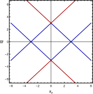
(a) $({B_{z}},M)=(3,0)$

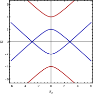
(b) $({B_{z}},M)=(3,1)$

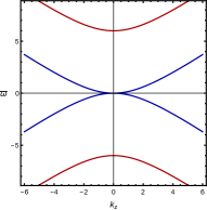
(c) $({B_{z}},M)=(3,3)$

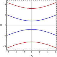
(d) $({B_{z}},M)=(3,5)$

Figure 1: (a)-(d):The band structure depends on $B_{z}/M$. The figure is in $(k_{z},\bar{\omega})$-space at $k_{x}=0,k_{y}=0$ slice. Here $\bar{\omega}=\omega+q\mu$.

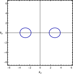
(a) $\bar{\omega}=1$

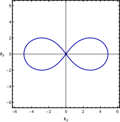
(b) $\bar{\omega}=2$

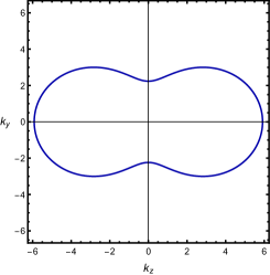
(c) $\bar{\omega}=3$

Figure 2: (a)-(c): The different $\bar{\omega}$ slices of the band structure at $k_{x}$=0 with $(\bar{B}_{z},M)=(3,1)$. The radius of circle decreases as $\bar{\omega}$ apparoches to 0. This result is the same for $k_{y}=0$ plane.

On the other hand, for $|{B_{z}}|<M$, a gap opens and its size is given by $2\Delta=2(M-{B}_{z})$. Figure 2 shows the top-view of the fermion spectrum with sections of Dirac cones which has the centers at the band crossing point of spectrum and it shrinks as we approach to $\bar{\omega}=0$, which implies the spectrum forms cone-structure near the band crossing points.

2.2 Holographic Fermions and their spectral function

To reproduce the above band structure of Weyl-semi metal in the holographic set up, we use a model which was first introduced in Y.liu2018

$$S =S_{1}+S_{2}+S_{int}$$ (4)

$$S_{1} =\int d^{5}x\sqrt{-g}i\bar{\Psi}_{1}(\Gamma^{a}D_{a}-m_{f}-iA_{a}\Gamma^{a})\Psi_{1},$$

$$S_{2} =\int d^{5}x\sqrt{-g}i\bar{\Psi}_{2}(\Gamma^{a}D_{a}+m_{f}+iA_{a}\Gamma^{a})\Psi_{2},$$

$$S_{\text{int}} =\int d^{5}x\sqrt{-g}(i\eta_{1}\Phi\bar{\Psi}_{1}\Psi_{2}+i\eta_{1}^{*}\Phi^{*}\bar{\Psi}_{2}\Psi_{1}),$$

where $\mathcal{D}_{M}=\partial_{M}+\frac{1}{4}\omega_{\underline{a}\underline{b}M}\Gamma^{\underline{a}\underline{b}}$ is the the covariant derivative and $\omega_{\underline{a}\underline{b}M}$ is the bulk spin connection, $\Gamma^{\underline{a}\underline{b}}=\frac{1}{2}[\Gamma^{\underline{a}},\Gamma^{\underline{b}}]$. $A_{a}$ is a gauge field with zero bulk mass and $\Phi$ is a scalar with $m^{2}_{\Phi}=-3$, breaking the time reversal symmetry(TRS) and chiral symmetry respectively. $M$ denotes bulk spacetime indices and $a,b$ denote bulk tangent space ones. In ref.  Y.liu2018 , zero temperature analysis was done. Here we will consider the finite temperature case. For this purpose, we take the Schwarzschild-$AdS_{5}$ background (6).

$$ds^{2} =-r^{2}f(r)dt^{2}+\frac{1}{r^{2}f(r)}dr^{2}+\frac{r^{2}}{L^{2}}d\vec{x}^{2}$$ (5)

$$f(r) =\frac{1}{L^{2}}\left(1-\frac{r_{0}^{4}}{r^{4}}\right)$$ (6)

where $L$ is $AdS_{5}$ radius and $r_{0}$ is the radius of the black hole which defines the temperature of boundary theory, where $T=f^{\prime}(r_{0})/4\pi=r_{0}/\pi L^{2}$. For $A_{z}$ and $\Phi$, we have the equations of motionLandsteiner2016 as follows:

$$A_{z}^{\prime\prime}+\left(\frac{3}{r}+\frac{f^{\prime}}{f}\right)A_{z}^{\prime}-\frac{2\Phi^{2}}{r^{2}f}A_{z} =0$$ (7)

$$\Phi^{\prime\prime}+\left(\frac{5}{r}+\frac{f^{\prime}}{f}\right)\Phi^{\prime}-\left(\frac{A_{z}^{2}}{r^{4}f}+\frac{m_{\Phi}^{2}}{r^{2}f}\right) =0$$ (8)

We can introduce the parameter $b$ and $M$ as a boundary condition for the fields $A_{z}$ and $\Phi$ which satisfy (7)

$$\lim_{r\rightarrow\infty}A_{z}(r)=b,\qquad\lim_{r\rightarrow\infty}r\Phi(r)=M$$ (9)

The specified parameter $(b,M)$ at the boundary can be reached by choosing proper horizon values of $A_{z}$ and $\Phi$, whose profles are shown in Figure 3 (a) and (b) respectively.

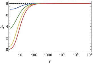
(a) Profile for $A_{z}$

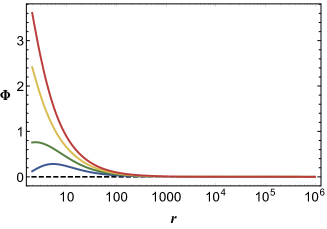
(b) Profile for $\Phi$

Figure 3: (a)(b) Profiles for $A_{z}$ and $\Phi$ where we fix $b=8$ and $T=2/\pi$. We use $M=0$, $3.3,$ $5.5$, $7.5$, $9.7$ for flat-dashed, blue, green, yellow, red (from top to bottom in (a) and from bottom to top in (b)).

We use the convention of $\Gamma$-matrices for fermion action as follows:

$$\Gamma^{\underline{t}}=\left(\begin{array}[]{cc}0&\gamma^{t}\\ \gamma^{t}&0\end{array}\right),\quad\Gamma^{\underline{i}}=\left(\begin{array}[]{cc}0&\gamma^{i}\\ -\gamma^{i}&0\end{array}\right),\quad\Gamma^{\underline{r}}\equiv\Gamma^{5}=\left(\begin{array}[]{cc}1&0\\ 0&-1\end{array}\right),\quad(\gamma^{t},\gamma^{i})=i(\mathbf{1}_{2},\sigma^{i})$$ (16)

where $\Gamma^{M}=e^{M}_{\underline{a}}\Gamma^{\underline{a}}$ and $e^{M}_{\underline{a}}$ is the inverse vielbein. Taking $\eta_{1}=1$, the equations of motions are given by

$$(\Gamma^{a}D_{a}-m_{f}-iA_{z}\Gamma^{z})\Psi_{1}-\Phi\Psi_{2} =0$$

$$(\Gamma^{a}D_{a}+m_{f}+iA_{z}\Gamma^{z})\Psi_{2}-\Phi\Psi_{1} =0$$ (17)

Expanding $\bar{\Psi}_{l}$ in Fourier space,

$$\Psi_{l}=(-gg^{rr})^{-1/4}e^{ik_{\mu}x^{\mu}}\psi_{l},$$ (18)

with $l=1,2$, the equations of motion for fermions become

$$\left(\sqrt{g^{rr}}\Gamma^{\underline{r}}\partial_{r}+\sqrt{g^{tt}}\Gamma^{\underline{t}}(-i\omega)+i\sqrt{g^{ii}}(k_{x}\Gamma^{\underline{x}}+k_{y}\Gamma^{\underline{y}}+(k_{z}\mp A_{z})\Gamma^{\underline{z}})+(-1)^{l}m_{f}\right)\psi_{l}-\Phi\psi_{3-l}=0$$ (19)

where we fixed $L=1$. Near the boundary $r\rightarrow\infty$, the spinors behave as

$$\psi_{1}^{T} =\left(A_{1}^{1}\ r^{m_{f}},A_{2}^{1}\ r^{m_{f}},A_{3}^{1}\ r^{-m_{f}},A_{4}^{1}\ r^{-m_{f}}\right)+\cdots,\qquad$$ (20)

$$\psi_{2}^{T} =\left(A_{1}^{2}\ r^{-m_{f}},A_{2}^{2}r^{-m_{f}},A_{3}^{2}\ r^{m_{f}},A_{4}^{2}\ r^{m_{f}}\right)+\cdots.$$ (21)

We have 8 variables of two first order dirac equations so that 8 “initial” conditions are required for radial evolution. Eliminating outgoing conditions at the horizon, the degrees of freedom are reduced to half. We choose four different initial conditions at the horizon and solve the equations to get near boundary values, which determines the retarded Green functions. We denote each initial conditions as I, II, III, IV respectively. We can construct the source and expectation matrices as follows:

$$\mathbf{A}=\left(\begin{array}[]{cccc}A_{1}^{1,I}&A_{1}^{1,II}&A_{1}^{1,III}&A_{1}^{1,IV}\\ A_{2}^{1,I}&A_{2}^{1,II}&A_{2}^{1,III}&A_{2}^{1,IV}\\ A_{3}^{2,I}&A_{3}^{2,II}&A_{3}^{2,III}&A_{3}^{2,IV}\\ A_{4}^{2,I}&A_{4}^{2,II}&A_{4}^{2,III}&A_{4}^{2,IV}\\ \end{array}\right),\qquad\mathbf{D}=\left(\begin{array}[]{cccc}-A_{1}^{2,I}&-A_{1}^{2,II}&-A_{1}^{2,III}&-A_{1}^{2,IV}\\ -A_{2}^{2,I}&-A_{2}^{2,II}&-A_{2}^{2,III}&-A_{2}^{2,IV}\\ A_{3}^{1,I}&A_{3}^{1,II}&A_{3}^{1,III}&A_{3}^{1,IV}\\ A_{4}^{1,I}&A_{4}^{1,II}&A_{4}^{1,III}&A_{4}^{1,IV}\\ \end{array}\right)$$ (30)

The Green function can be obtained by $\mathcal{G}_{R}=i\Gamma^{t}\mathbf{D}\mathbf{A}^{-1}$. See Appendix for more details. The spectral function is defined as the trace of the imaginary part of the retarded Green function:

$$A(\omega,\vec{k})=\text{Tr}\left(\text{Im}\left[\mathcal{G}_{R}(\omega,\vec{k})\right]\right).$$ (31)

Figure  4 shows the spectral density for this model. For $b_{z}>M$, band crossing exists and the distance between the two Weyl points becomes shorter as $M$ increases, and finally gap is open when $M>M_{c}$. Notice that $M_{c}\simeq b_{z}$ in holography, which is similar to the QFT result apart from the line broadening due to the interaction and temperature effects. See Figure 4 and 5.

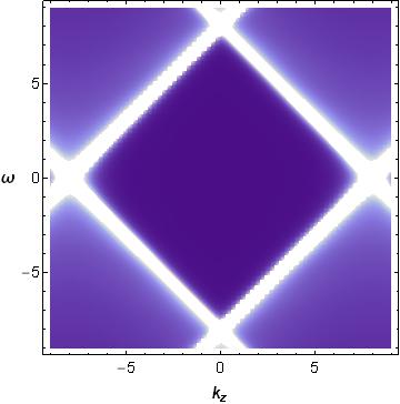
(a) $(b,M)=(8,0)$

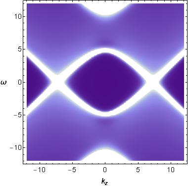
(b) $(b,M)=(8,3.3)$

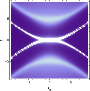
(c) $(b,M)=(8,7.5)$

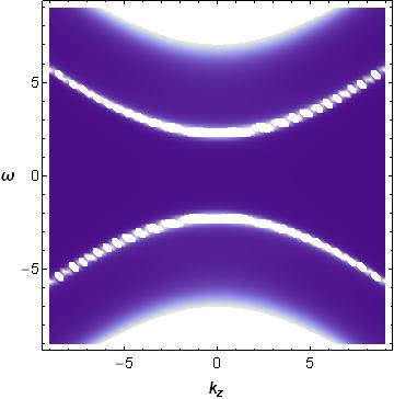
(d) $(b,M)=(8,9.7)$

Figure 4: (a)-(d):Spectral densities on $(k_{z},\omega)$-space with $k_{x}=k_{y}=0$ at $T=2/\pi$. Separation between the Weyl points is approximately $2\sqrt{b^{2}-M^{2}}$.

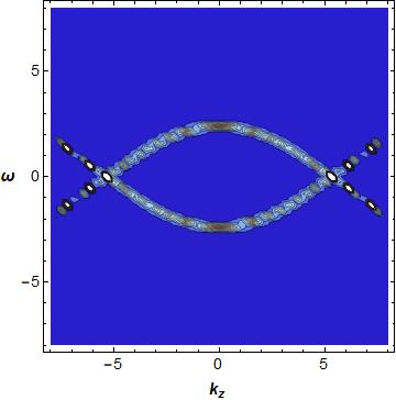
(a) $T=2/\pi$

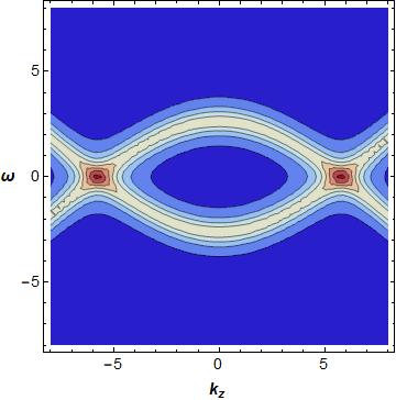
(b) $T=10/\pi$

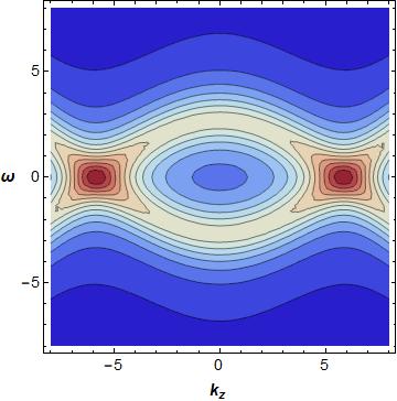
(c) $T=20/\pi$

Figure 5: (a)-(c): As temperature increases, spectrum broadens. Color code denotes the spectral height. We used $k_{x}=k_{y}=0$ and $(b,M)=(8,3.3)$.

However, we emphasize that the critical value of $M/b$ for the given $b$ is not exactly the same as $1$. The figure 6 shows the difference.

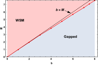
Figure 6: Phase diagram in $(b,M)$ space. We used $T=2/\pi$. Unlike the field theory, $M_{c}/b=1$ holds only approximately. Dashed line is for $b=M$.

3 Stability of Topology

3.1 Topological invariants from Green function

We study topology of holographic Weyl semi-metal (WSM) model using the topological Hamiltonian Wang2014 ; Wang2013

$$\mathcal{H}_{t}=-\mathcal{G}_{R}^{-1}(\omega=0,\vec{k}),$$ (32)

which contains all the effects of interaction and temperature. We can get eigenvectors from this topological hamiltonian so that we can define Berry connection,

$$\mathcal{A}_{\mathbf{k}}=i\sum_{j}\langle n_{\mathbf{k},j}|\partial_{\mathbf{k}}|n_{\mathbf{k}j}\rangle$$ (33)

where $n_{\mathbf{k}}^{j}$ are eigenvectors for $\mathcal{H}_{t}$ in momentum space and $j$ runs over all occupied bands. The Berry phase $\gamma$ is defined by Berry1984

$$\gamma=\oint_{\mathcal{C}}\mathcal{A}_{\mathbf{k}}\cdot d\mathbf{k}=\int_{\mathcal{S}}\mathbf{\Omega}_{\mathbf{k}}\cdot d\mathbf{S}$$ (34)

where $\mathcal{S}$ is a 2-dimensional surface whose boundary is $\mathcal{C}$, a closed loop, and $\Omega_{i}=\epsilon_{ijl}\left(\partial_{k_{j}}\mathcal{A}_{k_{i}}-\partial_{k_{i}}\mathcal{A}_{k_{j}}\right)$. Since the momentum space is 3-dimensional, we could take another surface $\mathcal{S}^{\prime}$ such that its boundary is also $\mathcal{C}$. Then the ambiguity free condition on the choice of the surface $\mathcal{S}$ gives the condition that

$$C=\frac{1}{2\pi}\oiint_{\mathcal{S}-\mathcal{S}^{\prime}}\mathbf{\Omega}_{\mathbf{k}}\cdot d\mathbf{S}=\iiint_{B}\nabla\cdot\nabla\times\mathcal{A}_{\mathbf{k}}$$ (35)

is an interger, a topological invariant known as Chern number. Here $B$ is a ball whose boundary is the closed surface $\mathcal{S}-\mathcal{S}^{\prime}$.

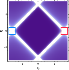
(a) Spectral function

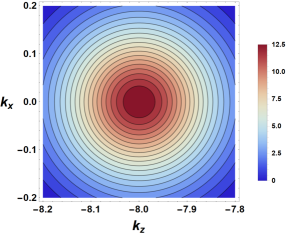
(b) Berry curvatures (LHS)

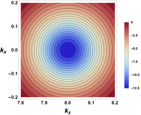
(c) Berry curvatures (RHS)

Figure 7: (a) Spectral function without scalar interaction. We used $(b,M)=(8,0)$ and $T=2/\pi$. $k_{x}=k_{y}=0$ fixed. (b),(c): Berry curvatures near $k_{z}=-8$ and $8$ at the plane ($k_{y}=-0.2$ , $\omega=0$), where topological numbers are still 1 and -1 respectively.

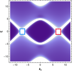
(a) Spectral function

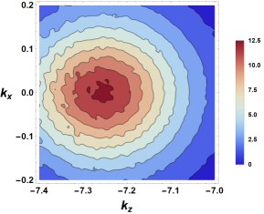
(b) Berry curvatures (LHS)

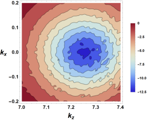
(c) Berry curvatures (RHS)

Figure 8: (a) Spectral function with scalar interaction. We used $(b,M)=(8,5.5)$ and $T=2/\pi$. $k_{x}=k_{y}=\omega=0$. (b),(c): Berry curvatures near $k_{z}=-7.26$ and $7.26$ at the plane ($k_{y}=-0.2$, $\omega=0$), where topological numbers are still 1 and -1 respectively.

In Figure 7(a), for example, if we take a closed surface surrounding a crossing point, then we get $C=1$ for the Weyl point at $k_{z}=-8$ and $C=-1$ for the one at $k_{z}=8$. Similarly, we get the Chern numbers for $(b_{z},M)=(8,5.5)$ of Figure 8. As you can see in Figure 4, the band crossing disappears when $b_{z}<M_{c}$ which is similar to QFT case. In the next subsection, we will try to understand what we found here in more analytic terms.

3.2 Stability of Topology in the presence of temperature and interaction

Figures 7(a) and 8(a) show that the band crossings and fuzziness in spectral lines simultaneously so that it is not clear whether there is a Weyl point with well defined topological number. Nevertheless, figures 7(b)(c) and 8(b)(c) show that there is an integer winding number for such fuzzy crossing. To understand such numerical result found in the last subsection, we first notice that the topological number of Weyl point depends only on the local singularity structure of the Berry phase, because in eq. (3.4), $\nabla\cdot\nabla\times\mathcal{A}_{\mathbf{k}}$ is zero unless it is a delta function whose support is inside the ball $B$. Therefore we only need to look at small neighborhood of the Weyl point, where only two bands are crossing. Therefore for the purpose of the topological number, we only need to look at $2\times 2$ matrix which describes one of the crossing point. This is equivalent to neglecting the highest or lowest branches in figure 1(b). Any ${2\times 2}$ matrix can be expanded in the following form

$$\mathcal{H}_{2\times 2}=\vec{b}(k)\cdot\vec{\sigma}+\Sigma\mathbf{1}_{2},$$ (36)

where $\Sigma=\Sigma^{\prime}+i\Sigma^{\prime\prime}$ is the self-energy. There are a few comments.
i) If $\Sigma$ were not the coefficient of the $1_{2}$ matrix, it would be a part of the momentum shift not energy shift and it would not be called as self-energy.
ii) The matrix becomes non-Hermitian due to the presence of the $\Sigma^{\prime\prime}$. It is well known that such non-hermicity is the result of the manybody interaction encoded in the 1-particle effective Hamiltonian: $\Sigma^{\prime\prime}$ is the sum of probabilities of the state of $\omega=0$ to go into all other states.
iii) Near a crossing point, $\vec{b}(k)\simeq v(\vec{k}-\vec{k}_{0})$ and $k_{0}$ is real. Equivalently, the matrix is non-Hermitian only by the presence of the self energy term.

$\Sigma^{\prime\prime}$ is what makes the spectral function and the ARPES data fuzzy. Below we can easily demonstrate the details why such fuzzy Fermi surface can still give well defined winding number. For simplicity, let $v=1$ and the Weyl point be at the origin so that $\vec{k}_{0}=0$. The solution of eigenvalue problem $\mathcal{H}\mbox{$|n_{k}\rangle$}=E\mbox{$|n_{k}\rangle$}$ are given by

$$\mbox{$|n_{k}^{1}\rangle$}=\frac{(-k_{x}+ik_{y},|\vec{k}|+k_{z})}{\sqrt{2|\vec{k}|(|\vec{k}|+k_{z})}},\quad\mbox{$|n_{k}^{2}\rangle$}=\frac{(|\vec{k}|+k_{z},k_{x}+ik_{y})}{\sqrt{2|\vec{k}|(|\vec{k}|+k_{z})}}$$ (37)

Berry potential given by Eq.(33) defines the vector potential of a magnetic monopole sitting at $\vec{k}=0$ whose field strength is given by $F_{12}={k_{z}}/{2k^{3}}$ whose integral over a small sphere $S_{0}$ around the $\vec{k}=0$ is $2\pi$, so that the chern number $C=\int_{S_{0}}\frac{F}{2\pi}=+1$.

The key observation is that there is no $\Sigma$ dependence in the expression of eigenvectors in Eq. (37). Therefore although the self energy term can make the Fermi surface fuzzy, it can not change the structure of Berry potential and hence can not change the topological structure.

One may want to consider the full $4\times 4$ matrix directly instead of looking at the crossing point, which reduced the effective Hamiltonian to $2\times 2$ matrix. The cost is rather expensive: the calculation is long so that even the result for the Berry potential takes a few pages to write. Nevertheless we can discuss some essence of the topological structure. We describe it in the appendix C.

4 Topolgical dipole in a holographic theory

In this section we consider a slightly modified model where some unusual but interesting phenomena happen.

4.1 Spectral functions and multiple band crossing

We start from the topological dipole model,

$$S_{1} =i\int_{\mathcal{M}}d^{5}x\sqrt{-g}\bar{\psi}_{1}\left(\Gamma^{M}\mathcal{D}_{M}-m-iA_{z}\Gamma^{5}\Gamma^{z}\right)\psi_{1}$$

$$S_{2} =i\int_{\mathcal{M}}d^{5}x\sqrt{-g}\bar{\psi}_{2}\left(\Gamma^{M}\mathcal{D}_{M}+m-iA_{z}\Gamma^{5}\Gamma^{z}\right)\psi_{2}$$

$$S_{int} =i\int_{\mathcal{M}}d^{5}x\sqrt{-g}(-\Phi\bar{\psi}_{1}\psi_{1}+\Phi\bar{\psi}_{2}\psi_{2})$$ (38)

where $S_{int}$ is the scalar interaction with $\phi\sim M/r$ near boundary. We take different sign for scalar interaction $\phi$ to make the term invariant under the parity transformation ($\vec{k}\to-\vec{k}$) Semenoff2012 .
The equations of motion are given by

$$(\cancel{\mathcal{D}}-m-\Phi-iA_{z}\Gamma^{5}\Gamma^{z})\psi_{1}=0$$

$$(\cancel{\mathcal{D}}+m+\Phi-iA_{z}\Gamma^{5}\Gamma^{z})\psi_{2}=0$$ (39)

We can decompose the bulk fermion field into two component spionors $\psi_{I+}$ and $\psi_{I-}$, which are eigenvectors of $\Gamma^{\underline{r}}$ with $I=1,2$ so that $\Gamma^{\underline{r}}\psi_{I\pm}=\pm\psi_{I\pm}$. Let

$$\psi_{I\pm}(r,x)=(-gg^{rr})^{-1/4}e^{ik_{\mu}x^{\mu}}\phi_{\pm}(r,k),\qquad\phi_{I\pm}=\left(\begin{array}[]{c}y_{I\pm}\\ z_{I\pm}\end{array}\right)$$ (42)

Using (42), the equations of motion for bulk fermion fields $\psi_{1}$ are given by

$$\sqrt{\frac{g_{ii}}{g_{rr}}}y_{1+}^{\prime}(r)-(m+\Phi)\sqrt{g_{ii}}y_{1+}(r)+(u_{+}-k_{z})y_{1-}(r)-(k_{x}-ik_{y})z_{1-}(r)= 0$$

$$\sqrt{\frac{g_{ii}}{g_{rr}}}z_{1+}^{\prime}(r)-(m+\Phi)\sqrt{g_{ii}}z_{1+}(r)-(k_{x}+ik_{y})y_{1-}(r)+(u_{-}+k_{z})z_{1-}(r)= 0$$

$$\sqrt{\frac{g_{ii}}{g_{rr}}}y_{1-}^{\prime}(r)+(m+\Phi)\sqrt{g_{ii}}y_{1-}(r)-(u_{+}+k_{z})y_{1+}(r)-(k_{x}-ik_{y})z_{1+}(r)= 0$$

$$\sqrt{\frac{g_{ii}}{g_{rr}}}z_{1-}^{\prime}(r)+(m+\Phi)\sqrt{g_{ii}}z_{1-}(r)-(k_{x}+ik_{y})y_{1+}(r)-(u_{-}-k_{z})z_{1+}(r)= 0$$ (43)

where $u_{\pm}=\omega\pm A_{z}$. One can get the equations of motion for $\psi_{2}$ by $m,\Phi\to-m,-\Phi$, which changes the chirality. At the boundary region ($r\rightarrow\infty$), the geometry becomes asymptotically $AdS_{5}$, so that Eqs. (43) have asymptotic solution as

$$y_{1+}(r) =A_{11}r^{m}+B_{11}r^{-m-1},\qquad y_{1-}(r)=C_{21}r^{m-1}+D_{11}r^{-m}$$

$$z_{1+}(r) =A_{12}r^{m}+B_{12}r^{-m-1},\qquad z_{1-}(r)=C_{22}r^{m-1}+D_{12}r^{-m}$$ (44)

$$\quad y_{2-}(r) =A_{21}r^{m}+B_{21}r^{-m-1},\qquad y_{2+}(r)=C_{21}r^{m-1}+D_{21}r^{-m}$$

$$z_{2-}(r) =A_{22}r^{m}+B_{22}r^{-m-1},\qquad z_{2+}(r)=C_{22}r^{m-1}+D_{22}r^{-m}$$ (45)

Here, we have two independent sets of equations. Each set needs four initial conditions, but as in WSM, we can fix half of them by choosing infalling condition at the horizon. Hence, it is required that we choose two independent initial conditions so that we can obtain two corresponding sets of source and expectation values to compute Greens function for each $\psi_{I}$. By denoting each initial conditions as (1), (2) respectively, we can construct the source and expectation matrices as $2\times 2$ matrices.

$$\mathbf{A}_{I}=\left(\begin{array}[]{cc}A_{I1}^{(1)}&A_{I1}^{(2)}\\ A_{I2}^{(1)}&A_{I2}^{(2)}\end{array}\right),\qquad\mathbf{D}_{I}=\left(\begin{array}[]{cc}D_{I1}^{(1)}&D_{I1}^{(2)}\\ D_{I2}^{(1)}&D_{I2}^{(2)}\end{array}\right)$$ (50)

The retarded Green function is defined by $\mathcal{G}_{I}^{R}=i\gamma^{t}\mathbf{D}_{I}\mathbf{A}_{I}^{-1}=-\mathbf{D}_{I}\mathbf{A}_{I}^{-1}$. However, since we know that each set of Greens function is independent, so we can construct Greens function matrices as $4\times 4$ block diagonalized matrices which is given by

$$\mathbf{G}^{R}=\left(\begin{array}[]{cc}\mathcal{G}_{1}^{R}&0\\ 0&-\mathcal{G}_{2}^{R}\end{array}\right)$$ (52)

where the $-$ sign in front of $\mathcal{G}_{2}^{R}$ represents the alternative quantization Laia2011 .

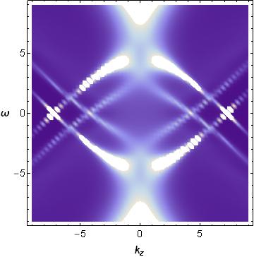
(a) $(b,M)=(8,5.5)$

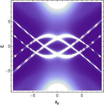
(b) $(b,M)=(8,7.5)$

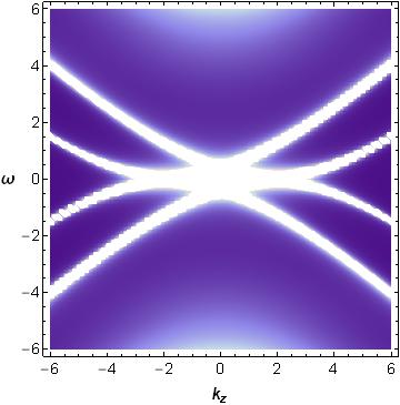
(c) $(b,M)=(8,11)$

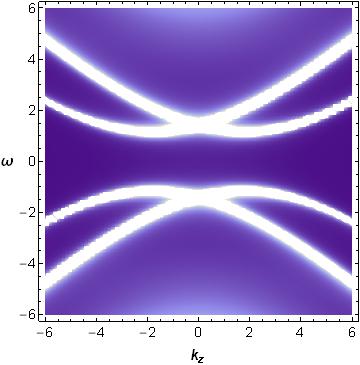
(d) $(b,M)=(8,12.7)$

Figure 9: (a)-(d): Band structure in $(k_{z},\omega)$ with $k_{x}=k_{y}=0$ of model in Eq. (4.1). We used $T=2/\pi$. Notice that at the critical point (c), it is not reduced to a Dirac point but to a higher Lifshitz point.

Comparing these spectral functions with holographic WSM case, one can see from Figure 9 that the outermost part of the spectrum evolves similarly to that of WSM case. As $M$ increases, the separation between outermost band-crossing points decreases and, after $M>M_{c}=4.3$, a gap opens and its size gets larger. However, there are crucial difference is that here we have multiple band-crossings. Each band forms cone-like structure.

As we increase the temperature, the spectrum goes fuzzy and the distance between adjacent spectra also increases with the position of the outermost part of spectrum fixed, which implies the number of crossing points near $\omega=0$ decreases. See Figure 10.

(a) $T=2/\pi$

(b) $T=10/\pi$

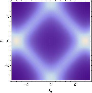
(c) $T=20/\pi$

Figure 10: (a)-(c):Temerpature effect on the spectral function when $(b,M)=(8,5.5)$ on $(k_{z},\omega)$-space with $k_{x}=k_{y}=0$.

4.2 Topological dipoles

We can also calculate the topological invariants of crossing points for this model. In this case, we have multiple crossing points unlike WSM, therefore we calculate Berry phase at each crossing points. For $k<0$, net topological invariants near the band crossing point are -1 while those for $k>0$ are 1. However, except for the outermost band crossing points, each poles of Berry curvature comes with its conjugate pair with opposite sign to make dipoles. See Figure 11. Notice that as we increase the temperature, the inner band-crossing points disappear (Figure 10). Since they depend on temperature sharply, we may consider that they are not stable. This is not surprising since two topological charges are so closely separated in momentum space, it is expected to be unstable for relatively small perturbations. From the Schrödinger potential picture, each band is induced by a confining well structure and disappearance in temperature means that the potential well is eaten by the black hole horizon as temperature increases. Notice that the leftmost crossing point has topological charge of $(-1,2)$ with small separation: it is a combination of the Weyl point having topological charge +1 and small separated dipole charges (-1,1).
To explain this better, we draw the contribution of $\psi_{1}$ and $\psi_{2}$ separately. For $\mathcal{G}_{1}^{R}$, there are 4 band crossing points. The rightmost one is the Weyl point with topological charge -1 and other three crossing points are dipoles with small separated -1 and +1 from left to right. Similarly for $\mathcal{G}_{2}^{R}$, there are 4 band crossing points and the leftmost one is the Weyl point with topological charge +1 and other three crossing points are dipoles with small separated -1 and +1 from left to right. Now combining these two, the position of dipole’s +1 charge happens to coincide with that of the Weyl point with charge +1.
Similar story goes on for the rightmost band crossing with opposite monople charge and the same dipole charge.

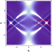
(a) Spectral function

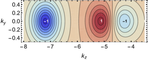
(b) Berry curvatures ($k_{z}<0$)

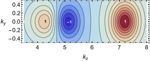
(c) Berry curvatures ($k_{z}>0$)

Figure 11: (a) Spectral function with $k_{x}=0,k_{y}=0$. Colored boxes are the regions where we draw Berry curvatures at Fermi level in (b) and (c) with $(b,M)=(8,5.5)$ and $T=2/\pi$. Each numbers in (b) and (c) represents winding number computed from Berry curvatures. As we can see from Fig 10, this dipole structure can disappear when temperature goes up.

Why dipole should come in this model? We can understand it as follows. Two fermions $\psi_{1},\psi_{2}$ are not mixing directly. So if one fermion has total Weyl charge +1, the other one has -1. Now if we draw spectral function for $\psi_{1}$, the shape has multiple crossings. Each crossing point has well defined topological charge. Now, the right-most crossing has -1 and unpaired, therefore all other 3 crossing points should come as a pair with topological charge (+1,-1) not to change the total charge $-1$. Similarly for $\psi_{2}$, the left-most crossing has +1 and unpaired, therefore every other ones should come as pairs. This is the reason why dipole should appear. Notice that if we sum two spectral function, then the total charge is summed to be 0. See figure 11.

5 Discussion

In this paper, we discussed the stability of the topological invariant of the interacting Weyl semi-metal at finite temperature and finite fermion mass. We utilize the holographic setup to calculate the Green’s functions and use the result to construct the effective Hamiltonian, which allows us to calculate the winding number of the Weyl points. We found that the topological winding number is stable even in the case where spectral function is fuzzy. The winding number turns out to be integer as far as there is band crossing at the Fermi level. Here we summarize the arguments why that is so: the topological number’s integrand is $ddA_{Berry}$ which is zero or delta function by Bianchi identity so that we only need to look at neighborhood of the Weyl point, where only two bands are crossing. Therefore it is enough to consider 2x2 matrix only. The interaction can change the spectral function to make it fuzzy by creating $\Sigma^{\prime\prime}$ but the latter is a coefficient of $\bf 1_{2}$ so that it can not modify the Eigenvectors which are the building blocks of the Berry potential determining the winding number. The formula of winding number is nothing but the reading machine of coefficient of that singularity, which can not be changed by smooth deformation of the theory by the interaction or temperature.

One subtle point at this moment is whether the interaction can develop the imaginary part of $b$ in Eq.(3.5). We numerically checked that the expression is still $b\sim(k-k_{0})$ near the crossing point. In fact, if there is a tiny imaginary part in $k_{0}$, one can show that topological number is zero. If a weak interaction or small temperature can induce imaginary part in $k$, it is equivalent to saying that topology is unstable for small deformation, which does not make sense. So we believe that the reality of $k_{0}$ is protected by a discrete symmetry. It is equivalent to say that effective Hamiltonian can be non-Hermitian only by the presence of imaginary self-energy term which is diagonal. In fact, there is no reason why interaction can generate arbitrary non-hermitian structure in the effective Hamiltonian. We want to comeback to the analysis of various discrete symmetry in the future.

We also defined a model where Weyl points are separated only by a small distance. We call it Topological Dipoles and study its topological invariant.

It would be very interesting to generalize this work to the case with more general type of interaction and also to Dirac materials in 2+1 dimension having other type singularities. For example, for the line node cases, multiple band crossings can define a new type of topological invariantAhn:2018qgz . New type of topological matter called “Fragile Topology” Po:2017uom ; PhysRevLett.120.266401 ; Hwang:2019nuf is also interesting possibility. We hope we comeback to these issues in future works.

Appendix

Appendix A Effective Schrödinger potential

We can define the effective bulk potential to analyze the role of scalar interaction for Dirac fermion in the bulk.

$$S_{D}=\int d^{5}x\sqrt{-g}\bar{\psi}(\Gamma^{M}\mathcal{D}_{M}-m-\phi)\psi+S_{bd}$$ (53)

Here, we use the pure AdS background which is given by

$$ds^{2}=-r^{2}dt^{2}+\frac{dr^{2}}{r^{2}}+r^{2}d\vec{x}^{2}$$ (54)

The Dirac equation in Fourier space is given by

$$r\Gamma^{r}\partial_{r}\psi+\frac{i}{r}\Gamma\cdot k\psi+2\Gamma^{r}\psi-(m+\phi)\psi=0$$ (55)

We can decompose the bulk fermion field into two component spionors $\psi_{+}$ and $\psi_{-}$, which correspond to eigenvectors of $\Gamma^{\underline{r}}$. That is, $\Gamma^{\underline{r}}\psi_{\pm}=\pm\psi_{\pm}$ and $\psi^{T}=\left(\psi_{+},\psi_{-}\right)$.
Then, equation (55) becomes coupled equations for $\psi_{\pm}$

$$\psi_{+}=-\frac{i\gamma\cdot k}{k^{2}}A(-m,-\phi)\psi_{-},\qquad\psi_{-}=\frac{i\gamma\cdot k}{k^{2}}A(m,\phi)\psi_{+}$$ (56)

where $k^{2}=\vec{k}^{2}-\omega^{2}$ and

$$A(m,\phi)=r\left(r\partial_{r}+2-m-\phi\right)$$ (57)

from which we obtain  Iqbal2009

$$k^{2}\psi_{+}=A(-m,-\phi)A(m,\phi)\psi_{+}$$ (58)

Changing the coordinate $r=1/z$, we substitute $\psi_{+}=r^{2}\psi$ to the equation 57. Then, we can get the Schrödinger form of the Dirac equation:

$$-\psi^{\prime\prime} +V_{eff}(z)\psi_{n}=E\psi$$

$$V(z) =\phi(z)+\frac{m(m-1)}{z^{2}}$$ (59)

We can extend the analysis to the finite temperature case, which has the Schwarzschild-$AdS_{5}$ background. We will not show the details of calculation for this since it is very complicated. We just show the effective bulk potential schematically for finite temperature case in Figure 12. As the temperature increases, the radius of black hole horizon increases so that the effective potential cannot form steep wall near the horizon. Hence, there cannot be a bound state, which gives a band structure.

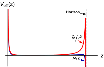
(a) $V_{\text{eff}}$ for different interaction

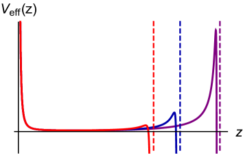
(b) Temperature evolution of $V_{\text{eff}}$

Figure 12: Schematic Schroedinger potential : (a) Comparison between $M/r$ and $\tilde{M}/r^{3}$. The coordinate used is $z=1/r$. (b) Temperature evolution of the effective potential in the bulk. Dashed lines are the event horizons at each temperature which moves in as T increases, and the potential changes from purple to red accordingly.

But, we cannot apply this analysis to our model because we have the momentum transfer in spectral densities and it might not be possible to construct the Schrodinger form of equations of motion. Even if it is possible to construct, we need to encode the momentum dependence on the effective potential, which should be done for each fixed momentum.

For the simple scalar interaction, there’s no momentum dependence, it is enough to calculate the case of $k=0$. Since $r$ corresponds to energy scale and $k=0$ means small energy scale so that the contribution of $V_{k}(r)$ at $r\sim 0$ is significant. On the other hands, for our model, which does have momentum dependence, the k dependence of the effective potential is significant. Hence the behavior of $V_{k}(r)$ at the finite $r$ is important.

Appendix B Holographic Greens function

We start from the simple probe fermion model,

$$S_{bulk}=\int_{\mathcal{M}}d^{5}x\sqrt{-g}i\bar{\psi}\left(\Gamma^{M}\mathcal{D}_{M}-m)\right)\psi$$ (60)

However, the action (60) is not sufficient and the boundary term is required to guarantee that the variational principle is well-defined. We will discuss later. The equations of motion are given by

$$(\cancel{\mathcal{D}}-m)\psi=0$$ (61)

Taking decomposition of the bulk fermion field into two component spinors $\psi_{+}$ and $\psi_{-}$ as previous section, we now expand the bulk-spinors in Fourier-space as following:

$$\psi_{\pm}(r,x)=(-gg^{rr})^{-1/4}e^{ik_{\mu}x^{\mu}}\phi_{\pm}(r,k),\qquad.$$ (62)

Setting $\phi_{\pm}^{T}=\left(y_{\pm},z_{\pm}\right)$, the eqs. of motion for bulk fermions are given by

$$\sqrt{\frac{g_{ii}}{g_{rr}}}y_{+}^{\prime}(r)-m\sqrt{g_{ii}}y_{+}(r)+(\omega-k_{z})y_{-}(r)-(k_{x}-ik_{y})z_{-}(r)= 0$$

$$\sqrt{\frac{g_{ii}}{g_{rr}}}z_{+}^{\prime}(r)-m\sqrt{g_{ii}}z_{+}(r)-(k_{x}+ik_{y})y_{-}(r)+(\omega+k_{z})z_{-}(r)= 0$$ (63)

$$\hbox{and }\qquad\sqrt{\frac{g_{ii}}{g_{rr}}}y_{-}^{\prime}(r)+m\sqrt{g_{ii}}y_{-}(r)-(\omega+k_{z})y_{+}(r)-(k_{x}-ik_{y})z_{+}(r)= 0$$

$$\sqrt{\frac{g_{ii}}{g_{rr}}}z_{-}^{\prime}(r)+m\sqrt{g_{ii}}z_{-}(r)-(k_{x}+ik_{y})y_{+}(r)-(\omega-k_{z})z_{+}(r)= 0,$$ (64)

using (62). Near the boundary ($r\rightarrow\infty$), the geometry becomes asymptotically $AdS_{5}$ spacetime, so that the equations of motion (64) have asymptotic behaviors as

$$y_{+}(r) =A_{1}r^{m}+B_{1}r^{-m-1},\qquad y_{-}(r)=C_{1}r^{m-1}+D_{1}r^{-m}$$

$$z_{+}(r) =A_{2}r^{m}+B_{2}r^{-m-1},\qquad z_{-}(r)=C_{2}r^{m-1}+D_{2}r^{-m}$$ (65)

Back to the boundary term, we take the variation to the bulk action (60),

$$\delta S_{bulk}=\int_{\partial\mathcal{M}}d^{4}x\sqrt{-h}\frac{i}{2}(\delta\bar{\psi}_{+}\psi_{-}+\bar{\psi}_{-}\delta\psi_{+}-\delta\bar{\psi}_{-}\psi_{+}-\bar{\psi}_{+}\delta\psi_{-})+\text{bulk part}$$ (66)

where $h=gg^{rr}$ and bulk part vanishes when the Dirac equations holds Laia2011 .
Since the Dirac equation is the first order differential equation, we cannot fix both $\psi_{+}$ and $\psi_{-}$ on the boundary simultaneously. Therefore we need the additional boundary to give well-difined variational principle:

$$S_{bdy}=\pm\frac{i}{2}\int_{\partial\mathcal{M}}d^{4}x\sqrt{-h}\bar{\psi}\psi=\pm\frac{i}{2}\int_{\partial\mathcal{M}}d^{4}x\sqrt{-h}(\bar{\psi}_{-}\psi_{+}+\bar{\psi}_{+}\psi_{-})$$ (67)

The sign can be determined such that we take positive(negative) sign when we fix the value of $\psi_{+}$($\psi_{-}$) at the boundary, where $\delta S_{bdy}$ cancels all the terms including $\delta\psi_{-}$ ($\delta\psi_{+}$) in $\delta S_{D}$. And this defines the standard(alternative) quantization. By using (65), the boundary action in (67) becomes

$$S_{bdy}\sim y_{-}z_{-}+y_{+}z_{+}=(A_{1}D_{1}+A_{2}D_{2})+\Sigma_{\pm}E_{\pm}r^{\pm 2m-1}+E_{2}r^{-2},$$ (68)

It seems that $S_{bdy}$ blows up at the boundary when $m>1/2$, but, it can be cancelled by introducing proper counter terms Ammon2010 , which do not have finite terms at the boundary. As we mentioned above, if we choose the standard quantization, we should fix $\psi_{+}$ at the boundary so that $A_{i}$ are the sources and $D_{i}$ are the expectation values. From now on, we will hold to this quantization rule. Therefore, if variables with $-$ index and those with $+$ in equations are not mixed such as $k_{x}=k_{y}=0$, the retarded Green’s function is given by

$$\mathcal{G}=\text{diag}\left(-\frac{D_{1}}{A_{1}},-\frac{D_{2}}{A_{2}}\right)\equiv\text{diag}(G_{+},G_{-})$$ (69)

In this paper, however, we should consider all $(\omega,\vec{k})$ space so that the variables in equations cannot be decoupled. Hence, we need to define the Green function in another way. We have 4 variables and each needs 1 initial condition, hence 4 initial conditions are required. By choosing infalling functions at the horizon, we can relates $y_{+}$ to $y_{-}$ and $z_{+}$ to $z_{-}$, which means there are only two dimensional space of initial condition. These are the pair of coefficients of infalling wave functions of $y_{+},z_{+}$ : Denote them $(y_{+}^{0},z_{+}^{0})$. Two independent basis vector of this space can be chosen as $(1,1)$ and $(1,-1)$. Let’s call them $\vec{e_{1}}$ and $\vec{e_{2}}$ respectively. For each $i$, $\vec{e_{i}}$ determines their counterpart at the horizon ($i.e$ $y_{-}^{0},z_{-}^{0}$) and one can integrate the equations of motion from the horizon to the boundary. Then, for each initial conditions $\vec{e_{i}}$, $i=1,2$, we get near-boundary solution

$$y_{+}^{(i)} =A_{1}^{(i)}r^{m}+B_{1}^{(i)}r^{-m-1},\qquad y_{-}^{(i)}=C_{1}^{(i)}r^{m-1}+D_{1}^{(i)}r^{-m}$$

$$z_{+}^{(i)} =A_{2}^{(i)}r^{m}+B_{2}^{(i)}r^{-m-1},\qquad z_{-}^{(i)}=C_{2}^{(i)}r^{m-1}+D_{2}^{(i)}r^{-m}$$ (70)

Since the choice of coefficients is arbitary, the general boundary solutions should be a linear combnination of the such solution with some coefficients. For example, $y_{+}=c_{1}y_{+}^{(1)}+c_{2}y_{+}^{(2)}$. For the general boundary solutions, its coefficients $X_{a}$, where $X=A,B,C,D$ are given by $X_{a}=\sum_{i}X_{a}^{(i)}c_{i}$. The matrix $\mathbf{X}$ is defined by the components $X_{a}^{(i)}$ where $a,i=1,2$ are the row index and columb index respectively. We can solve for $c_{i}$: by definition, $\vec{c}=\mathbf{A}^{-1}\vec{A}$ for $X=A$. Green function can be derived from the relation between $\vec{D}$ and $\vec{A}$:

$$\vec{D}\equiv\mathcal{S}\vec{A}=\mathbf{D}\mathbf{A}^{-1}\vec{A}\quad\Rightarrow\quad\mathcal{G}_{R}\equiv i\gamma^{t}\mathcal{S}=-\mathbf{D}\mathbf{A}^{-1}$$ (71)

Appendix C Topology in 4 by 4 Hamiltonian model for WSM

First let’s assume following form of the effective Hamiltonian:

$$\mathcal{H} =-\mathcal{G}_{R}^{-1}(0,\vec{k})=\left(\begin{array}[]{cc}\vec{b}_{1}(k)\cdot\vec{\sigma}+\Sigma\mathbf{1}_{2}&m\mathbf{1}_{2}\\ m\mathbf{1}_{2}&\vec{b}_{2}(k)\cdot\vec{\sigma}+\Sigma\mathbf{1}_{2}\end{array}\right)$$ (74)

where $\vec{b}_{1}(k)\simeq v(\vec{k}-\vec{k}_{0})$ near the right Weyl point and $\vec{b}_{2}(k)\simeq-v(\vec{k}+\vec{k}_{0})$ near the left Weyl point. In fact, if we start from (4), the effective hamiltonian Eq.(32) numerically calculated always takes above form. There are a few steps to prove that the presence of topological number.

1. For small $m$ and near $k_{0}$, taking the expansion in $m$ gives us $\vec{B}=\nabla\times\vec{A}(k)=\frac{1}{2}\frac{\vec{p}}{|p|^{3}}+{\cal O}{(m^{2})}$ with $p=k-k_{0}$.

2. $\nabla\cdot\vec{B}=0$ off the Weyl point by the Bianchi identity,.

3. From 1 and 2, $\nabla\cdot\vec{B}=2\pi\delta(\vec{k}-\vec{k_{0}})$. Therefore $C=\frac{1}{2\pi}\int_{S_{0}}B\cdot dS$ is non-zero integer or zero depending on whether $S_{0}$ contains Weyl point $k_{0}$ or not.

4. The topological number $C$ is independent of $m$, therefore we can set $m=0$ for the purpose of calculating the Chern number. For $m=0$, we only need to handle $2\times 2$ matrix, which was already done above.

One can prove that topological structure is intact as far as $k_{0}$ is real. The fact that $k_{0}$ does not get imaginary part is due to the discrete symmetry P (parity) and T(Time reversal). Even in the case where the Fermi sea disappears due to the interaction, such crossing point is located exactly at the $\omega=0$ by T symmetry. When $k_{0}$ gets imaginary numbers, the monopole singularity is smoothed out in the real domain and the chern number becomes 0. This is expected because the topology of a manifold and the singularity of the harmonic function defined on it is equivalent and because the singularity of the monopole field $\sim 1/k^{2}$ is resolved.

Note that the figure 4 is for finite temperature. The position of the Weyl point is not changed compared with the Minkowski space, the non-interacting case, but there is finite line broadening. Figures 7 and 8 are the spectral functions at different temperature and for different fermion mass $M$, where one can see that the topological number is the same integer value in spite of very different broadening widths. Increasing temperature makes the spectral lines even fuzzier leaving the topological invariant still fixed.

Therefore the topological structure is very stable under the variation of temperature and interactions in holographic theory. The argument here can be generalized to other class of topological matter although we focus here on Weyl semi-metal Hamiltonian.

In appexdix C, we consider more general cases where $m\mathbf{1}_{2}$ is replaced by $m\mathbf{1}_{2}+\vec{q}\cdot\vec{\sigma}$ and classify the cases where Weyl points exist.

Now, what if the off-diagonal interaction is added to the $\mathcal{H}_{0}$ so that the effective Hamiltonian becomes

$$\mathcal{H}=\left(\begin{array}[]{cc}(\vec{p}-\vec{p_{0}})\cdot\vec{\sigma},&m\mathbf{1}_{2}+\vec{q}\cdot\vec{\sigma}\\ m\mathbf{1}_{2}+\vec{q}\cdot\vec{\sigma},&-(\vec{p}+\vec{p_{0}})\cdot\vec{\sigma}\end{array}\right)$$ (77)

where $\vec{q}=(q_{1},q_{2},q_{3})$. For Weyl points, Eigenvalues should vanish only at two distinct points with $k_{x}=k_{y}=0$. It is difficult to get explicit form of Eigenvalues of $\mathcal{H}$ in general. Therefore we classify the cases and study one by one.

C.1 $m=0$

• $q_{3}=0$
  When $q_{3}=0$ and $q_{1},q_{2}\neq 0$, the dispersion relation is given by

  $$(\omega-k_{z})^{2}=k_{0}^{2}+q_{1}^{2}+q_{2}^{2}$$ (78)

  which implies that two Weyl points always exist at $(k_{x},k_{y},k_{z})=(0,0,\pm\sqrt{k_{0}^{2}+q_{1}^{2}+q_{2}^{2}})$. See figure 13(a).

  

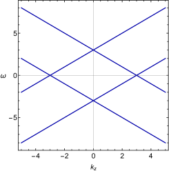
  (a) $(k_{0},q_{1},q_{2})=(2,1,2)$

  

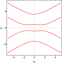
  (b) $(k_{0},q_{1},q_{3})=(2,1,2)$

  Figure 13: Dispersion curve for $m=0$ (a) $q_{1},q_{2}\neq 0$, (b) $q_{1},q_{3}\neq 0$

• $q_{3}\neq 0$ and $q_{1}q_{2}=0$
  When $q_{2}=0$, the dispersion relation is given by

  $$\omega^{2}=k_{z}^{2}+k_{0}^{2}+q_{1}^{2}+q_{3}^{2}\pm 2\sqrt{k_{z}^{2}(k_{0}^{2}+q_{1}^{2})+k_{0}^{2}q_{3}^{2}}$$ (79)

  In this case, there is no Weyl point and this hamiltonian is gapped. See figure 13(b). This result is symmetric for $q_{1}$ and $q_{2}$. One should notice that only when $q_{1}=q_{2}=0$ one can have Weyl point in the presence of $q_{3}$.

• $q_{3}\neq 0$ and $q_{1}=q_{2}=0$, the dispersion relation becomes

  $$\omega=\pm\Big{(}k_{0}\pm\sqrt{k_{z}^{2}+q_{3}^{2}}\Big{)}.$$ (80)

  In this case, the system has two Weyl points if $k_{0}>q_{3}$, or gapful if $k_{0}<q_{3}$.

C.2 $m\neq 0$

When both $m$ and $q_{3}$ are non-zero we can not get analytic expression for the dispersion curve unless $q_{1}=q_{2}=0$.

• $q_{3}=0$

When $q_{3}=0$, the dispersion curve is given by

$$\omega=\pm\left(\sqrt{k_{z}^{2}+m^{2}}\pm\sqrt{k_{0}^{2}+q_{1}^{2}+q_{2}^{2}}\right)$$ (81)

which implies that Weyl points exist at $k_{z}^{2}=k_{0}^{2}-m^{2}+q_{1}^{2}+q_{2}^{2}$ if $k_{0}^{2}+q_{1}^{2}+q_{2}^{2}>m^{2}$ holds and gapful otherwise. See figure 14(a)

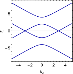
(a) $(m,k_{0},q_{1},q_{2})=(1,2,1,2)$

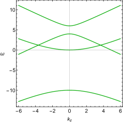
(b) $(m,k_{0},q_{3})=(2,5,3)$

Figure 14: Dispersion curve for $m>0$. (a) $q_{1},q_{2}\neq 0$ and (b) $q_{1},q_{2}=0$

• $q_{3}\neq 0$ and $q_{1}=q_{2}=0$

When $q_{1}=q_{2}=0$, the dispersion curve is given by

$$(\omega-k_{0})^{2}=k_{z}^{2}+(m\pm q_{3})^{2}$$ (82)

In this case, we have 4 roots for $\omega=0$ and as you can see from dispersion curve, the Weyl points are lifted due to the shift of $\omega$ by $k_{0}$. See figure 14(b). If both $m$ and $q_{3}$ are non-zero, we could get analytic expression for the dispersion curve only when $q_{1}=q_{2}=0$. Therefore we leave it future work for such case.

- (1) C. L. Kane and E. J. Mele, topological order and the quantum spin hall effect, Physical Review Letters 95 (sep, 2005) .
- (2) X.-L. Qi, T. L. Hughes and S.-C. Zhang, Topological field theory of time-reversal invariant insulators, Physical Review B 78 (nov, 2008) .
- (3) X.-L. Qi, T. L. Hughes, S. Raghu and S.-C. Zhang, Time-reversal-invariant topological superconductors and superfluids in two and three dimensions, Physical Review Letters 102 (may, 2009) .
- (4) S. Raghu, X.-L. Qi, C. Honerkamp and S.-C. Zhang, Topological mott insulators, Physical Review Letters 100 (apr, 2008) .
- (5) E. Witten, Three lectures on topological phases of matter, Riv.Nuovo Cim. 39 (2016) no.7, 313-370 (2015) , [http://arxiv.org/abs/1510.07698v2].
- (6) M. Freedman, A. Kitaev, M. Larsen and Z. Wang, Topological quantum computation, Bulletin of the American Mathematical Society 40 (2003) 31–38.
- (7) C. Nayak, S. H. Simon, A. Stern, M. Freedman and S. D. Sarma, Non-abelian anyons and topological quantum computation, Reviews of Modern Physics 80 (2008) 1083.
- (8) L. Fidkowski and A. Kitaev, Effects of interactions on the topological classification of free fermion systems, Physical Review B 81 (apr, 2010) .
- (9) V. Gurarie, Single-particle green’s functions and interacting topological insulators, Physical Review B 83 (feb, 2011) .
- (10) Z. Wang, X.-L. Qi and S.-C. Zhang, Topological invariants for interacting topological insulators with inversion symmetry, Physical Review B 85 (apr, 2012) .
- (11) K. Landsteiner, Y. Liu and Y.-W. Sun, Quantum phase transition between a topological and a trivial semimetal from holography, Physical Review Letters 116 (feb, 2016) .
- (12) K. Landsteiner and Y. Liu, The holographic weyl semi-metal, Physics Letters B 753 (feb, 2016) 453–457.
- (13) Y. Liu and Y. Sun, Topological invariants for holographic semimetals, JHEP 1810 (2018) 189 (2018) .
- (14) P. Goswami and S. Tewari, Axionic field theory of (3+1)-dimensional weyl semi-metals, Phys. Rev. B 88, 245107 (2013) (2013) .
- (15) D. Colladay and V. A. Kostelecký, Lorentz-violating extension of the standard model, Physical Review D 58 (oct, 1998) .
- (16) Z. Wang and S. C. Zhang, Topological invariants and ground-state wave functions of topological insulators on a torus, Phys. Rev. X 4, no. 1, 011006 (2014) (2014) .
- (17) Z. Wang and B. Yan, Topological hamiltonian as an exact tool for topological invariants, Journal of Physics: Condensed Matter 25 (mar, 2013) 155601.
- (18) M. V. Berry, Quantal phase factors accompanying adiabatic changes, Proceedings of the Royal Society A: Mathematical, Physical and Engineering Sciences 392 (mar, 1984) 45–57.
- (19) G. W. Semenoff, Chiral symmetry breaking in graphene, Physica Scripta T146 (jan, 2012) 014016.
- (20) J. N. Laia and D. Tong, A holographic flat band, Journal of High Energy Physics 2011 (nov, 2011) .
- (21) J. Ahn, D. Kim, Y. Kim and B.-J. Yang, Band Topology and Linking Structure of Nodal Line Semimetals with Z2 Monopole Charges, Phys. Rev. Lett. 121 (2018) 106403, [1803.11416].
- (22) H. C. Po, H. Watanabe and A. Vishwanath, Fragile Topology and Wannier Obstructions, Phys. Rev. Lett. 121 (2018) 126402, [1709.06551].
- (23) J. Cano, B. Bradlyn, Z. Wang, L. Elcoro, M. G. Vergniory, C. Felser et al., Topology of disconnected elementary band representations, Phys. Rev. Lett. 120 (Jun, 2018) 266401.
- (24) Y. Hwang, J. Ahn and B.-J. Yang, Fragile Topology Protected by Inversion Symmetry: Diagnosis, Bulk-Boundary Correspondence, and Wilson Loop, 1905.08128.
- (25) N. Iqbal and H. Liu, Real-time response in AdS/CFT with application to spinors, Fortschritte der Physik 57 (apr, 2009) 367–384.
- (26) M. Ammon, J. Erdmenger, M. Kaminski and A. O’Bannon, Fermionic operator mixing in holographic p-wave superfluids, Journal of High Energy Physics 2010 (may, 2010) .