Eigenfunctions of Galactic Phase Space Spirals from Dynamic Mode Decomposition

Abstract

We investigate the spatiotemporal structure of simulations of the homogeneous slab and isothermal plane models for the vertical motion in the Galactic disc. We use Dynamic Mode Decomposition (DMD) to compute eigenfunctions of the simulated distribution functions for both models, referred to as DMD modes. In the case of the homogeneous slab, we compare the DMD modes to the analytic normal modes of the system to evaluate the feasibility of DMD in collisionless self gravitating systems. This is followed by the isothermal plane model, where we focus on the effect of self gravity on phase mixing. We compute DMD modes of the system for varying relative dominance of mutual interaction and external potential, so as to study the corresponding variance in mode structure and lifetime. We find that there is a regime of relative dominance, at approximately $4:1$ external potential to mutual interaction where the DMD modes are spirals in the $(z,v_{z})$ plane, and are nearly un-damped. This leads to the proposition that a system undergoing phase mixing in the presence of weak to moderate self gravity can have persisting spiral structure in the form of such modes. We then conclude with the conjecture that such a mechanism may be at work in the phase space spirals observed in Gaia Data Release 2, and that studying more complex simulations with DMD may aid in understanding both the timing and form of the perturbation that lead to the observed spirals.

1 Introduction

Astrometric and radial velocity surveys of the Milky Way such as SEGUE (Yanny et al., 2009), RAVE (Steinmetz et al., 2006), LAMOST Cui et al. (2012), and Gaia Data Release 2 (GDR2) (Gaia Collaboration et al., 2018a, b), have revealed a panoply of phase space structures in the Galactic stellar disc. In the vicinity of the Sun, these structures include vertical asymmetries in the local stellar number density (Widrow et al., 2012; Yanny & Gardner, 2013; Bennett & Bovy, 2018), vertical bulk motions of disc stars (Widrow et al., 2012; Williams et al., 2013; Carlin et al., 2013; Quillen et al., 2018; Gaia Collaboration et al., 2018b) and phase spirals in $z-v_{z}$ projections of the stellar distribution function (DF) (Antoja et al., 2018). In addition, there is evidence for corrugations of the disc (Xu et al., 2015) at distances of $10$ to $15$ kpc from the Galactic centre. At even larger radii, there is the prominent warp (Binney, 1992; Sellwood, 2013), as well as evidence for disc stars kicked up to large Galactic latitudes (Price-Whelan et al., 2015). Taken together, these observations point to a disk in a state of disequilibrium.

Perhaps the most intriguing of the aforementioned structures are the phase spirals in the radial velocity subsample of GDR2 (Antoja et al., 2018). They were first seen by selecting stars in an arc of about 8 degrees in Galactic azimuth and $200\,{\rm pc}$ in Galactocentric radius centered on the Sun and plotting the number density, mean $v_{\phi}$ or mean $v_{R}$ across the $z-v_{z}$ plane. The spirals have now been studied as a function of position within the disc, action variables, and stellar properties (Bland-Hawthorn et al., 2019b; Laporte et al., 2019; Li & Shen, 2019).

A heuristic explanation of the spirals is that a local bend in the disc phase mixes due to the anharmonic nature of the vertical potential (Antoja et al., 2018), while coupling of the vertical and in-plane motions then leads to the $v_{R}$ and $v_{\phi}$ spirals (Schönrich & Binney, 2018; Darling & Widrow, 2018). In the simplest implementation of this picture, one treats stars as test particles in a fixed potential. This model seems to capture the basic features of the spirals and allows one to estimate the time at which the initial perturbation that gave rise to them took place (Antoja et al., 2018). Nevertheless, it leaves several questions unanswered, which include the following: What perturbed the disc? Can we point to a singular event that drove the disc from equilibrium or is the disc in a perpetual state of disequilibrium? What is the underlying DF of the perturbed disc. The phase spirals are likely the de-projection of the number count asymmetry along the $z$ axis mentioned above to the $z-v_{z}$ plane. Can we understand the spirals as the projection of some higher dimensional structure?

A number of candidates have been proposed as the agent of disequilibrium. For example, the disc may have been perturbed by a passing satellite galaxy or dark matter subhalo with the Sagittarius dwarf a prime suspect (Laporte et al., 2019; Bland-Hawthorn et al., 2019b). On the other hand, the buckling of the stellar bar has been shown to generate phase spirals in simulations of a Milky Way-like galaxy (Khoperskov et al., 2019).

The more challenging problem is to discern the phase space DF. Tremaine (1999) stressed the idea that the dimensionality of the DF can change via phase mixing. For example, a satellite galaxy that is being tidally disrupted by the gravitational potential of its host galaxy changes from a six-dimensional structure to a three-dimensional stream. Tremaine (1999) showed that one can relate changes in the phase space structure of a system to the eigenvalues of the Hessian matrix for the Hamiltonian. In principle, the method could be applied to phase mixing in a Galactic disc.

The main drawback of the phase mixing arguments is that they ignore the self-gravity of the perturbation, which is clearly important for the development of both bending and density waves in the disc. In short, when a local region of the disc is displaced from the midplane, it exerts a perturbing force on the unperturbed disc that, at least in linear theory, is the same order as the restoring force pulling it back into the midplane due to the unperturbed disc (Hunter & Toomre, 1969). A striking example of the importance of self-gravity can be found in the toy model simulations of bending waves in Darling & Widrow (2018) (Figure 7). Of course, self-gravity is built into the simulations of Laporte et al. (2019); Bland-Hawthorn et al. (2019a) and Khoperskov et al. (2019).

These considerations suggest that phase mixing and self-gravity are competing effects. A particularly simple toy model in which this competition plays out is the one-dimensional slab. This system can be thought of as an idealized disc in which all of the structure is in the direction normal to the midplane. It can be studied using linear perturbation theory as well as 1D N-body simulations (Mathur, 1990; Weinberg, 1991; Widrow & Bonner, 2015). For an isolated system there exists a trivial zero frequency normal mode corresponding to the displacement of the system relative to the midplane as well as a continuous spectrum of modes. If an external restoring force is included, then the displacement mode no longer has zero frequency. Moreover, if the DF for the system is truncated in energy, then gaps open up in the continuum and one has the possibility of additional discrete modes. In general, perturbations of the system will involve a mixture of discrete modes and modes from the continuum where the former should lead to eternal oscillations while the latter phase mix on time-scales related to the gradient of the frequency across the continuum. In his N-body simulations, Weinberg (1991) found that it was difficult to excite the discrete modes, presumably because power was leaking into nearby parts of the continuum where phase mixing was occurring. He did find that the system exhibited oscillations that were long-lived as compared to its dynamical time.

A similar situation arises when one applies linear perturbation theory to a simple two-dimensional model for a galactic disc comprising concentric, rotating, razor-thin rings. This model, which was employed to study warps, is in some sense complementary to the slab model. If the system is isolated or embedded in a spherical halo, there is a zero-frequency mode corresponding to the tilting of the system as a whole. As with the slab model, there is also a continuous spectrum of modes (Hunter & Toomre, 1969; Sparke & Casertano, 1988). On the other hand, if the system is embedded in a flattened halo, then the tilt mode becomes non-trivial and, in fact, has features similar to those seen in warped galaxies (Sparke & Casertano, 1988). That said, the discrete warp mode found by Sparke & Casertano (1988) does not appear to exist when the ring-model disc is immersed in a live halo (Binney et al., 1998).

Evidently, a proper treatment of stellar dynamics in galactic discs must capture the physics of both phase mixing and self-gravity. In this paper, we propose that dynamic mode decomposition (DMD) can provide a route to achieving this end. DMD was developed in the field of computational fluid dynamics to study problems involving turbulent flows and jets (Schmid, 2010), and is closely related to Koopman theory (see Mezić (2005) and Rowley et al. (2009)) It is essentially a dimensionality reduction algorithm for time-series data with the aim of identifying the dominant eigenfunctions of a system. At first glance, eigenvalue methods, which generally require a linear operator, would seem to be incompatible with the nonlinear problem at hand. The idea is to “lift” the dynamics from the state space, where the dynamics is governed by nonlinear physics to a space where the dynamics is described by a linear (generally infinite dimensional) operator, usually referred to as the Koopman operator (Mezić, 2005). DMD can provide a finite dimensional approximation of this operator comprised of dominant eigenfunctions of the system. One is left with a low-dimensional space in which the evolution of the system may be represented linearly and the dominant structure readily studied. DMD is similar in aim to the methods in Tremaine (1999) in terms studying structure and its dimensionality. However since DMD is data driven, the inclusion of self gravity is much simpler as compared to the process of obtaining an appropriate action space Hamiltonian.

The layout of the paper is as follows. In Section 2 we present a summary of the DMD method and its connection with the theory of small oscillations. In Section 3 we apply DMD to an N-body simulation of the homogeneous slab model. This system exhibits small oscillations about an equilibrium state, which can be compared to analytically derived normal modes (Antonov, 1971; Kalnajs, 1973). We then turn, in Section 4, to the isothermal plane, which serves as a simple model for the vertical structure of a Galactic disc. Our isothermal plane simulations are constructed so that we can adjust the relative importance of self-gravity and an external potential. In this case DMD is used to study the interplay between phase mixing and oscillatory modes. In doing so it helps elucidate the physics of $z-v_{z}$ phase spirals and the importance of self-gravity. In Section 5 we suggest a path forward for using DMD with full six-dimensional simulation data. Finally, we conclude with a summary and discussion in Section 6.

2 Characteristic Oscillations

2.1 Small Oscillations

Consider a classical system with $n$ degrees of freedom described by the generalized phase space coordinates $\mathbf{x}=(\mathbf{q},\mathbf{p})^{T}$. In the neighborhood where oscillations of the system are small, we consider a linearized Hamiltonian $H(\mathbf{q},\mathbf{p})=U(\mathbf{q})+K(\mathbf{p})$, where both the potential $U(\mathbf{q})$ and the kinetic energy $K(\mathbf{p})$ are quadratic forms (Arnold, 1989):

$$U(\mathbf{q})=\tfrac{1}{2}\mathbf{q}^{T}\mathbf{Bq},\ \ K(\mathbf{p})=\tfrac{1}{2}\mathbf{p}^{T}\mathbf{C}\mathbf{p}.$$ (1)

In this case, the equations of motion can be written as a linear operator equation,

$$\frac{d\mathbf{x}}{dt}=\boldsymbol{\mathcal{A}}\mathbf{x},$$ (2)

where

$$\boldsymbol{\mathcal{A}}=\begin{pmatrix}\mathbf{0}&\mathbf{C}\\ -\mathbf{B}&\mathbf{0}\\ \end{pmatrix}.$$ (3)

The solution is then given in terms of the eigendecomposition of $\boldsymbol{\mathcal{A}}$,

$$\mathbf{x}(t)=\sum_{j}b_{j}\boldsymbol{\phi}_{j}e^{\omega_{j}t},$$ (4)

where $\boldsymbol{\phi}_{j}$ and $\omega_{j}$ are the eigenvectors and eigenvalues of $\boldsymbol{\mathcal{A}}$, that is, $\boldsymbol{\mathcal{A}}\phi_{j}=\omega_{j}\phi_{j}$ and the coefficients $b_{j}$ are determined from the initial conditions.

2.2 Dynamic Mode Decomposition

In this section, we provide a compact overview of DMD, which draws from the introductory chapters of Kutz et al. (2016). We consider a nonlinear dynamical system that is described by some general state vector $\mathbf{x}(t)$, which does not necessarily belong to a Hamiltonian system. The goal of DMD is to determine the best-fit linear model for the non-linear dynamics. The key idea is that over a sufficiently short time interval $\Delta t$, the dynamics of the system can be approximately described by a linear system of equations of the form given in equation 2 with a solution given by equation 4.

With these considerations in mind, we draw $m$ discrete time samples $\mathbf{x}_{j}$ from the system with a sampling period of $\Delta t$. We then construct the equivalent discretized system of equations

$$\mathbf{x}_{j+1}\approx\mathbf{A}\mathbf{x}_{j},$$ (5)

where the discrete-time map is given by $\mathbf{A}=e^{\mathcal{A}\Delta t}$. We emphasize here that the states $\mathbf{x}_{j}$ need not be coordinates of the system, but can be any set of observables.

In general, the operator $\mathbf{A}$ is not known but is approximated from the data. To do so, we construct the data matrix

$$\mathbf{X}=\begin{pmatrix}|&|&&|\\ \mathbf{x}_{1}&\mathbf{x}_{2}&...&\mathbf{x}_{m-1}\\ |&|&&|\\ \end{pmatrix},$$ (6)

and the time shifted data matrix

$$\mathbf{X^{\prime}}=\begin{pmatrix}|&|&&|\\ \mathbf{x}_{2}&\mathbf{x}_{3}&...&\mathbf{x}_{m}\\ |&|&&|\\ \end{pmatrix}.$$ (7)

Our system of equations can then be approximated with the matrix equation

$$\mathbf{X^{\prime}}\approx\mathbf{A}\mathbf{X}.$$ (8)

From this, $\mathbf{A}$ is estimated by minimizing the matrix norm, $||\mathbf{X^{\prime}}-\mathbf{A}\mathbf{X}||$, which yields the result

$$\mathbf{A}=\mathbf{X^{\prime}}\mathbf{X}^{+}.$$ (9)

Here, $\mathbf{X}^{+}$ denotes the Moore-Penrose pseudo-inverse of $\mathbf{X}$, which can be computed via singular value decomposition (SVD). As in Press et al. (2002) the SVD of $\mathbf{X}$ is defined by the relation $\mathbf{X}\approx\mathbf{U}\mathbf{\Sigma}\mathbf{V}^{\dagger}$ where ^† denotes the Hermitian conjugate transpose, $\mathbf{\Sigma}$ holds the singular values along its diagonal, and $\mathbf{U}$ and $\mathbf{V}$ are comprised of left and right orthonormal vectors respectively. Using the SVD, we have that $\mathbf{X}^{+}=\mathbf{V}\mathbf{\Sigma}^{-1}\mathbf{U}^{\dagger}$, with which the discrete-time map becomes

$$\mathbf{A}\approx\mathbf{X^{\prime}}\mathbf{V}\mathbf{\Sigma}^{-1}\mathbf{U}^{\dagger}.$$ (10)

Our next goal is to obtain the eigendecomposition of $\mathbf{A}$ as we did with $\mathbf{\mathcal{A}}$ in Section 2.1 to facilitate understanding the time evolution of the system in terms of dominant modes. In the spirit of principal component analysis, we assume that the dominant structure of the system may be described by $r<m$ modes. Recall that in principle component analysis, when a data matrix $\mathbf{X}$ possesses low dimensional structure, it may be reasonably approximated in a basis spanned by the $r$ column vectors in $\mathbf{U}$ of its SVD corresponding to the $r$ largest singular values. We therefore work with the projection of $\mathbf{A}$ into this $r$-dimensional subspace,

$$\tilde{\mathbf{A}}=\mathbf{U}^{\dagger}\mathbf{A}\mathbf{U}=\mathbf{U}^{\dagger}\mathbf{X^{\prime}}\mathbf{V}\mathbf{\Sigma}^{-1}.$$ (11)

By working with this projection, we drastically reduce the dimension of the discrete-time map, making its eigendecomposition computationally tractable despite the typically large data matrices. Doing so also improves the numerical stability of the pseudo-inverse of $\mathbf{X}$.

We now determine the eigenvalues and eigenvectors of $\tilde{\mathbf{A}}$. That is, we solve the equation $\tilde{\mathbf{A}}\mathbf{\Xi}=\mathbf{\Xi}\mathbf{\Lambda}$ where $\mathbf{\Lambda}$ is a diagonal matrix whose elements $\lambda_{j}$, $j=1,\dots r$ are the eigenvalues of $\tilde{\mathbf{A}}$, and $\mathbf{\Xi}$ is a matrix whose columns are the corresponding eigenvectors. To a good approximation, the $r$ most dominant eigenvalues of $\mathbf{A}$ are the $\lambda_{j}$ while the corresponding eigenvectors, which are often referred to as the DMD modes, are given by

$$\mathbf{\Phi}=\mathbf{X^{\prime}}\mathbf{V}\mathbf{\Sigma}^{-1}\mathbf{\Xi}=\begin{pmatrix}|&|&&|\\ \boldsymbol{\phi}_{1}&\boldsymbol{\phi}_{2}&...&\boldsymbol{\phi}_{r}\\ |&|&&|\\ \end{pmatrix}.$$ (12)

(For a detailed explanation and proof, see Tu et al. (2014).)

We now have all of ingredients necessary to write a series solution for the state of the system. The solution takes the form of equation 4, where as before $b_{j}$ are the initial amplitudes of the modes, given by $\mathbf{b}=\mathbf{\Phi}^{+}\mathbf{x}_{1}=\big{(}b_{1}\ ...\ b_{r}\big{)}^{T}$, and the frequencies are $\omega_{j}=\ln(\lambda_{j})/\Delta t$.

In general, $\lambda_{j}$ can be real, imaginary, or complex. The case $\lambda_{j}=1$ ($\omega_{j}=0$) corresponds to a time-independent mode and arises, for example, when one has a system that is oscillating about some equilibrium configuration. Imaginary $\lambda_{j}$ indicates a pure oscillating mode, what would usually be referred to as a normal or true mode of the system. Real $\lambda_{j}$ correspond to pure growing or decaying modes while complex $\lambda_{j}$ correspond to pure damped or growing oscillations. It is often convenient to split the modal decomposition into terms with real and complex eigenvalues. In particular, for a system described by some real function, the DMD eigenvalues come in complex conjugate pairs and the associated pairs of modes combine to yield real contributions in the modal decomposition.

We conclude this Section with a few remarks that relate DMD back to our earlier discussion of small oscillations in Section 2.1. When DMD is applied to a system that is solvable by the method of characteristic oscillations, say, a linearized system with $n$ degrees of freedom, it is natural to construct the data matrices from measurements of the $n$ generalized coordinates. One can then use the full discrete-time map $\mathbf{A}$ and expect to obtain the $n$ characteristic or normal modes of the system. The power of DMD becomes manifest when we consider complex, nonlinear systems where simple analytic methods fail. In such cases, we can construct the data matrices using some convenient set of observables, where the $r$ modes that one obtains are data rather than model driven.

3 The Homogeneous Slab

In this section, we apply DMD to the linear oscillations of a self-gravitating, collisionless system of particles about its equilibrium state. For pedagogical reasons, we take the equilibrium state to have uniform density within a prescribed distance from the origin. The system was first studied by Antonov (1971) and Kalnajs (1973). Its simplicity derives from the fact that in the equilibrium state, all particles undergo simple harmonic motion about the origin. Furthermore, the linear modes are discrete and purely oscillatory. In addition, the DF for these modes can be expressed as elementary functions of the phase space variables, which we take to be $z$ and $v_{z}$. By contrast, the oscillations of the isothermal plane considered in Section 4 include discrete and continuum modes, which can be purely oscillatory or damped and can only be derived numerically using complex analysis.

3.1 Analytic Considerations

By Jeans theorem, the DF for an equilibrium, one-dimensional system can be written as a function of the sole integral of motion, the energy $E=v_{z}^{2}/2+\psi(z)$. For the homogeneous slab, the DF is given by

$$f_{0}^{K}(E)=\begin{cases}2^{-3/2}\pi^{-2}\big{(}1-E\big{)}^{-\frac{1}{2}},\quad 0<E<1\\ 0,\quad\text{otherwise},\end{cases}$$ (13)

where the superscript $K$ signifies that this is the original Kalnajs model. We use dimensionless units such that the velocity dispersion, extent of the system in $z$, and Newton’s constant are all set to unity (Widrow & Bonner, 2015). In these units, the system has uniform density $\rho_{0}=(2\pi)^{-1}$ in the region $|z|\leq 1$, and zero density for $|z|>1$. All particles undergo simple harmonic motion about $z=0$ at a frequency of $\Omega_{c}=\sqrt{2}$. Thus the transformation to action angle variables is analytic and has a simple geometric interpretation:

$$z=E^{\frac{1}{2}}\cos(\theta),\ \ v_{z}=(2E)^{\frac{1}{2}}\sin(\theta)~{}.$$ (14)

Note that the phase space distribution is bounded by the ellipse, $E=z^{2}+v_{z}^{2}/2=1$.

The normal modes of the system can be derived directly from a set of density-potential pairs (Antonov, 1971; Kalnajs, 1973; Widrow & Bonner, 2015), which removes the usual need for the Kalnajs matrix method . Letting $P_{n}$ be the Legendre polynomial of degree $n$, the density and potential of $j\text{th}$ mode are written

$$\psi_{j}^{K}(z)=N_{j}\big{(}P_{j+1}(z)-P_{j-1}(z)\big{)},$$ (15)

and

$$\rho_{j}^{K}(z)=-\tfrac{1}{4\pi}\,\tfrac{j(j+1)}{1-z^{2}}\,N_{j}\big{(}P_{j+1}(z)-P_{j-1}(z)\big{)},$$ (16)

where $N_{j}=\big{(}\frac{2\pi}{2j+1}\big{)}^{\frac{1}{2}}$.

We focus here on the lowest order even and odd parity modes, which correspond to $j=1$ and $j=2$, respectively. From equation 15 we have

$$\psi_{1}^{K}(z) =\frac{3N_{1}}{2}\big{(}z^{2}-1\big{)}$$ (17)

$$\psi_{2}^{K}(z) =\frac{5N_{2}}{2}\big{(}z^{3}-z\big{)}.$$

With use of the appropriate Legendre polynomials and trigonometric identities, these are written in terms of the action-angle variables as

$$\psi_{1}^{K}(z) =\frac{3N_{1}}{2}\bigg{(}E\cos^{2}(\theta)-1\bigg{)}$$ (18)

$$\psi_{2}^{K}(z) =\frac{5N_{2}}{2}\bigg{(}\frac{E^{\frac{3}{2}}}{4}\cos(3\theta)+\bigg{(}\frac{3E^{\frac{3}{2}}}{4}-E^{\frac{1}{2}}\bigg{)}\cos(\theta)\bigg{)}.$$

Since both potentials are even in the periodic variable $\theta$, we may write them as even Fourier series, distinguishing the even and odd parity modes by their Fourier coefficients. That is,

$$\psi_{1}^{K}(z) =\sum_{n>0}\psi_{1,n}\cos(n\theta),\ \ n\in 2\mathbb{Z}+1$$ (19)

$$\psi_{2}^{K}(z) =\sum_{n>0}\psi_{1,n}\cos(n\theta),\ \ n\in 2\mathbb{Z}.$$

Comparison of equations 18 and 19 implies that the relevant Fourier coefficients are

$$\psi_{1,2} =\frac{3N_{1}E}{4},$$ (20)

$$\psi_{2,1} =\frac{5N_{2}}{2}\bigg{(}\frac{3E^{\frac{3}{2}}}{4}-E^{\frac{1}{2}}\bigg{)},\ \ \psi_{2,3}=\frac{5N_{2}}{2}\bigg{(}\frac{E^{\frac{3}{2}}}{4}\bigg{)}.$$

As in Widrow & Bonner (2015) we can also write the mode DFs as a Fourier series

$$Re\{f_{j}\}=\frac{df_{0}}{dE}\sum_{n}\frac{2\psi_{j,n}\cos(n\theta)}{2-\omega^{2}/n^{2}},$$ (21)

where the sum over $j$ is restricted to even values for the even parity modes, and odd values for the odd parity modes. We therefore have

$$Re\{f_{1}^{K}(E,\theta)\} =\frac{df_{0}^{K}}{dE}\frac{\psi_{1,2}\cos(2\theta)}{1-\omega^{2}/8}$$ (22)

$$Re\{f_{2}^{K}(E,\theta)\} =\frac{df_{0}^{K}}{dE}\bigg{(}\frac{2\psi_{2,1}\cos(n\theta)}{2-\omega^{2}}+\frac{2\psi_{2,3}\cos(3\theta)}{2-\omega^{2}/9}\bigg{)},$$

where the derivative term $df_{0}^{K}/dE$ is restricted to the domain $0\leq E<1$, as it is infinite at the boundary $E=1$. Finally, we obtain $\rho_{j}$ by integrating equation 22 over $v_{z}$. Consistency with equation 16 then leads to a $j$’th order polynomial equation $\omega^{2}$, which can be solved to obtain $\omega/\Omega_{c}=1.73$ for $f_{1}$, and $\omega/\Omega_{c}=1.07,2.80$ for $f_{2}$ (Kalnajs, 1973). Note that in general, there are $j$ modes for a given $j$ and we therefore have a double series of modes.

3.2 DMD Modes of the Homogeneous Slab

We next simulate the homogeneous slab model. The initial conditions are a sample of $N=2\times 10^{5}$ equal mass particles drawn from the equilibrium DF. The system is first evolved for 80 dynamical times. As we will see, during this period it settles into a new equilibrium state in which the discontinuities in the DF and density are smoothed out. Note that the only source of perturbations is the shot noise from the finite number of particles. The system is then evolved for an additional 80 dynamical times and it is this period of the simulation that we use for our DMD analysis.

Snapshots comprise the DF $f(z,\,v_{z})$ estimated on a $150\times 150$ grid in the $z-v_{z}$ plane for $\{|z|,|v_{z}|\}<2$ and are sampled at a frequency of $10\Omega_{c}$. To estimate the DF, we take the number of particles in each phase space cell, multiply by the particle mass, and divide by the phase space volume of the cell. Each snapshot is then reshaped into a single column vector. The set of snapshots are then combined to yield the data matrices $\mathbf{X}$ and $\mathbf{X}^{\prime}$. These matrices have shapes $22,500\times 800$ and therefore satisfy one of the conditions of DMD, namely that they be “tall and skinny” Kutz et al. (2016). The DMD solution is then computed with a rank of $r=35$.

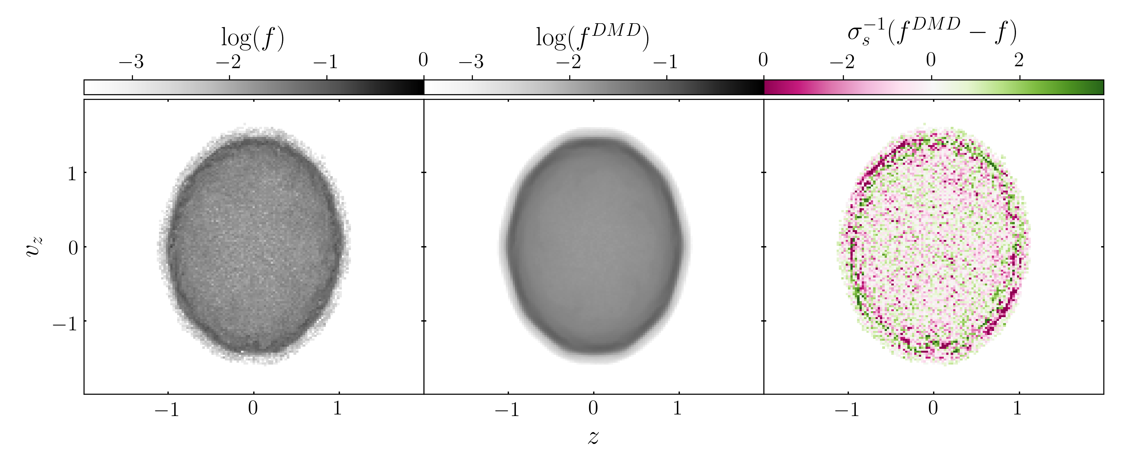
Figure 1: A single snapshot of the slab simulation, the computed DMD solution, and the corresponding residual. We show only a single snapshot here, as the snapshots of the system do not vary in a visually observable way in the studied time interval. The error is divided by the magnitude of shot noise fluctuations, $\sigma_{s}$ to highlight the error in the DMD solution independent of noise in the simulation.

Fig. 1 shows a single snapshot from halfway through the simulation period used for the DMD analysis. In the first panel, we show an estimate for the DF. As noted above and discussed in more detail below, the discontinuity at $E=1$ is smoothed out. In the middle panel we show the DMD solution while in the final panel, we show the difference between the two in units of the uncertainty, estimated from root-N statistics. The residual structure is dominantly random and the errors in each bin lie within the expected range of fluctuations. There are larger residuals for $E\sim 1$, which we believe correspond to high order structure in the simulation that is not accurately captured by our relatively low-rank DMD solution. Since the residuals lie within the statistical expectation, we take the DMD model to be accurate enough to be proceed.

Following Section 2.2, and noting that we have a real valued observable, we split the DMD series solution into separate sums over real and complex modes:

$$f^{DMD}(z,v_{z},t)=\sum_{j=1}^{r-q}b_{j}\boldsymbol{\phi}_{j}e^{\omega_{j}t}+\sum_{k=-\frac{q}{2}}^{\frac{q}{2}}b_{k}\boldsymbol{\phi}_{k}e^{\omega_{k}t},$$ (23)

where the the $q$ complex eigenfunctions and eigenvalues satisfy $\boldsymbol{\phi}_{k}^{*}=\boldsymbol{\phi}_{-k}$ and $\lambda_{k}^{*}=\lambda_{-k}$ respectively. The linear combination of two modes that belong to a conjugate pair and are weighted by complex amplitudes $a_{k}(t)=b_{k}e^{\omega_{k}t}$ is real. That is, for a conjugate pair of DMD modes, we define the corresponding mode of the DF to be

$$f_{j}^{DMD}(z,v_{z},t)=\sum_{l=\pm k}b_{l}\boldsymbol{\phi}_{l}e^{\omega_{l}t}.$$ (24)

In Fig. 2 we show the signal energy of the mode amplitudes as a function of mode frequency, alongside lines indicating the theoretical frequencies of the slab model from Kalnajs (1973). Reassuringly, agreement between the DMD mode frequencies and the expected ones is excellent.

We now focus on a few particular DMD modes beginning with the highest amplitude mode. This mode has zero frequency, as seen in Fig. 2 and corresponds to the equilibrium state. Its energy distribution $f_{0}^{DMD}(E)$, found by integrating the DF over the angle variable $\theta$, is shown in Fig. 3. As mentioned above, the discontinuity in the energy distribution near $E=1$ is smoothed out. (Note that in constructing $f_{0}^{DMD}(E)$ we use the potential for the original homogeneous slab model, which turns out to be an excellent approximation to the potential for the smoothed distribution.)

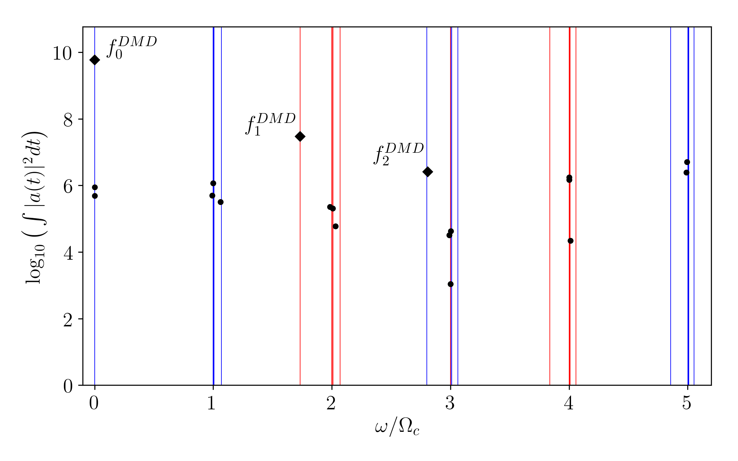
Figure 2: Mode amplitude signal energy as a function of mode frequency. The black points correspond to DMD modes, and the lines are plotted at the theoretical frequencies of the Kalanjs slab model, with blue and red lines indicating even and odd parity respectively.

We next turn to the $\omega/\Omega_{c}=1.73,~{}j=1$ and $\omega/\Omega_{c}=2.80,~{}j=2$ modes. The analytic DFs for these modes are given in equation 22 and plotted in the middle panels of Fig. 4. The frequencies and amplitudes of the corresponding DMD modes are shown as large diamonds in Fig. 2 while the DMD modes themselves are plotted on the lefthand panels of Fig. 4. The main difference between the analytic DFs and the DMD modes is found just beyond $E=1$. Evidently, the DMD modes extend beyond $E=1$ while the analytic modes have a sharp edge there.

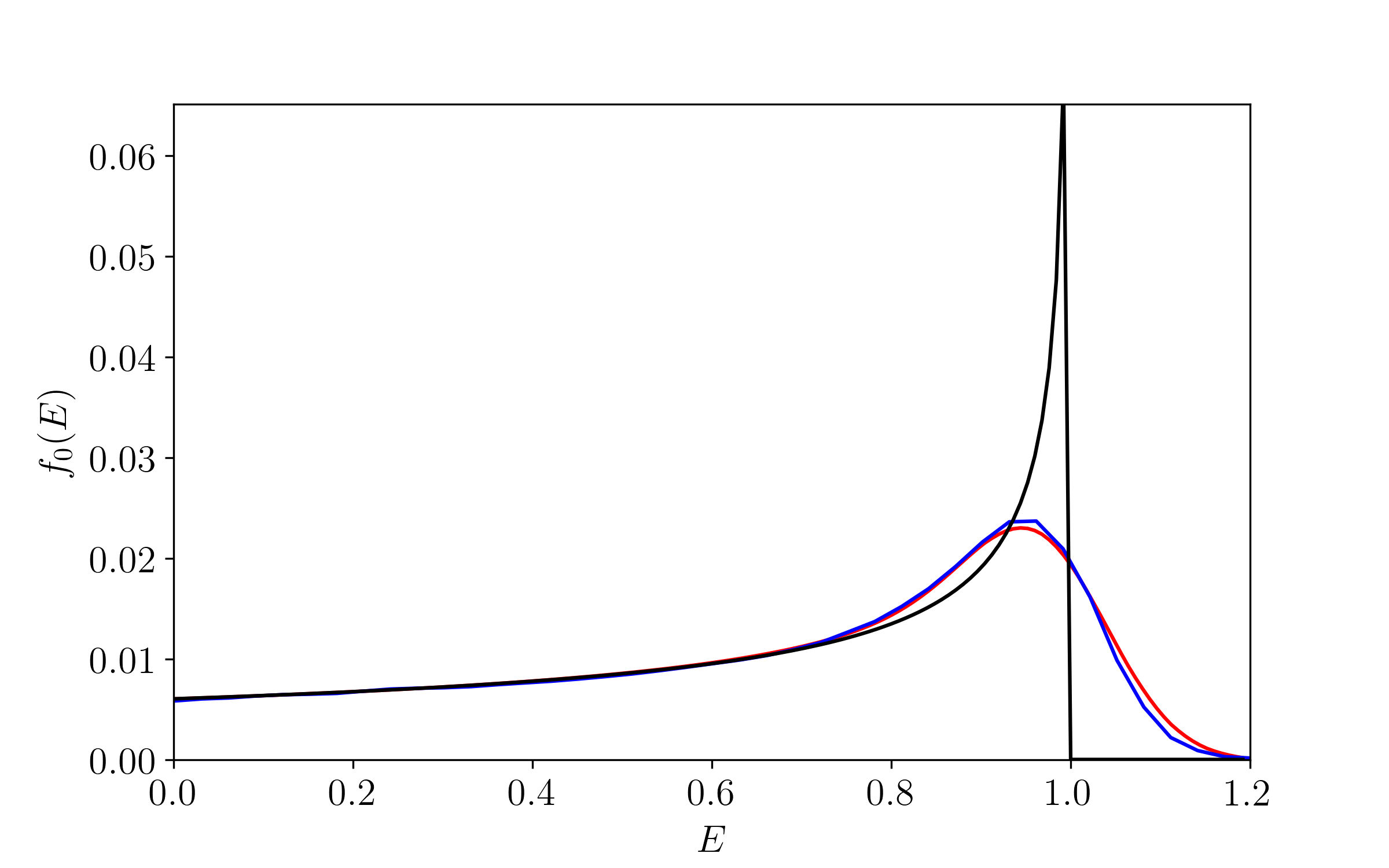
Figure 3: Equilibrium DFs of the Kalnajs model (black), modified slab model (red), and the equilibrium DMD mode (blue). In computing $f_{0}^{DMD}(E)$ we have assumed the potential corresponding to the fitted density in equation 25.

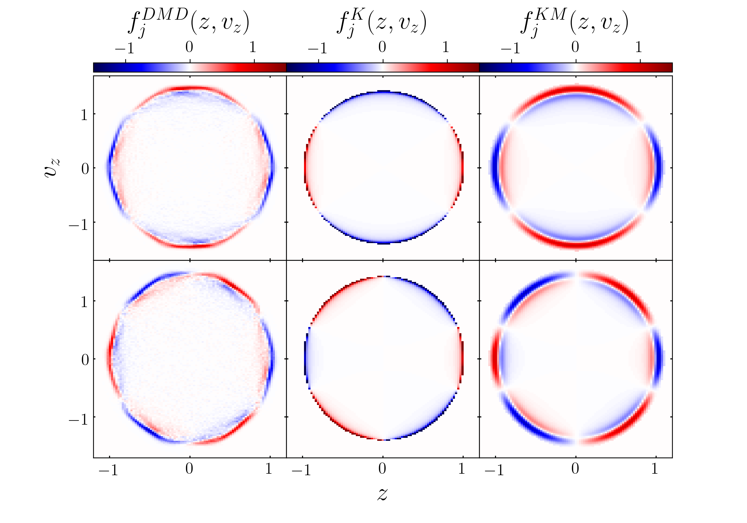
Figure 4: Mode DFs of the DMD solution, the Kalnajs model, and the modified slab model. The normalization of the three models has been adjusted, and a rotation has been applied to the DMD modes for easy comparison.

3.2.1 Modified Slab Model

The discrepancies between DMD modes and analytic linear modes are clearly related to the $df_{0}/dE$ factor in equation 21. To explore the discrepancies further we return to our discussion of the zero frequency mode. As seen in Fig. 3, the sharp peak and discontinuity in $f(E)$ is smoothed out in the simulation. Likewise, the discontinuity in the density is also smoothed out. In fact, the density is well represented by the fitting formula

$$\rho_{0}^{KM}(z)=\frac{1}{4\pi}\bigg{(}1+erf{\bigg{(}\frac{1-|z|}{a}\bigg{)}}\bigg{)},$$ (25)

where the constant $a$ corresponds to the width of the transition region from $\rho_{0}=1/2\pi$ to $0$. For our simulation, we find a best-fit value of $a=0.037$. A smoothed out homogeneous slab model was presented in Leeuwin et al. (1993), although with a different functional form that what we use here. The potential associated with equation 25 can be derived from the Greens function for the Poisson equation in one dimension and can be expressed in terms of special functions.

Armed with this density-potential pair, we can then derive the associated equilibrium DF via the Abel transform

$$f(E)=-\frac{\sqrt{2}}{\pi}\int_{E}^{\infty}\frac{d\rho}{d\psi}\frac{d\psi}{\big{(}\psi-E\big{)}^{\frac{1}{2}}}.$$ (26)

The integrand in equation 26 approaches infinity when the energy and potential take on similar values. To remedy this, we make a change of variable letting $\gamma=\sqrt{2}(\psi-E)^{\frac{1}{2}}$, such that equation 26 becomes

$$f(E)=-\frac{2}{\pi}\int_{0}^{\infty}\frac{d\rho}{d\psi}d\gamma.$$ (27)

This integral must be evaluated numerically. The resulting DF is shown in Fig. 3, together with $f(E)$ for the homogeneous slab (equation 13) and the zeroth order DMD mode. As can be seen in this figure, the equilibrium distribution function of the modified slab has a finite and smooth derivative that changes sign in the neighborhood of $E=1$, but otherwise behaves similarly to that of the homogeneous slab model.

The righthand panels of Fig. 4 show the linear modes (equation 21) with $df_{0}/dE$ calculated from our smoothed DF. They are qualitatively similar to the DMD modes in that they change sign for $E\simeq 1$ and extend beyond the $E=1$ ellipse.

In summary, for this simulation, DMD has constructed a set of modes that include a zeroth order equilibrium distribution and linear oscillatory perturbations in a manner reminiscent of perturbation theory. However, unlike perturbation theory, the zeroth order and linear perturbations are calculated simultaneously and directly from simulation data, without direct appeal to the underlying physics (i.e., the linearized Boltzmann and Poisson equations). In addition, the DMD analysis does not require that the perturbations be small. Indeed, the analysis is perfectly applicable to simulations of nonlinear systems.

4 The Isothermal Plane

We now consider the isothermal plane model, first developed by Spitzer (1942) and Camm (1950), and used as an approximation for the vertical structure of a stellar disc by Freeman (1978) and van der Kruit & Searle (1981).

4.1 Model Details

In this model, the equilibrium DF and density are given by

$$f_{\rm eq}\left(z,\,v_{z}\right)=\frac{\rho_{0}}{\left(2\pi\sigma_{z}^{2}\right)^{1/2}}e^{-E_{z}/\sigma_{z}^{2}}$$ (28)

and

$$\rho_{\rm eq}(z)=\rho_{0}e^{-\psi(z)/\sigma_{z}^{2}},$$ (29)

where $E_{z}$ is the vertical energy, and $\sigma_{z}$ is the velocity dispersion. For an isolated, self-gravitating system, the density and potential must satisfy the Poisson equation and we have

$$\psi_{\rm eq}(z)=2\sigma_{z}^{2}\ln{\cosh{\left(z/z_{0}\right)}},$$ (30)

where $\rho_{0}=\sigma_{z}^{2}/2\pi Gz_{0}^{2}$.

Here we split the gravitational force into two parts: a time-independent part, coming from masses external to the disc, such as the dark halo, and a live part coming from the disc itself. That is, we write the potential as

$$\psi(z,t)=\psi_{\rm ext}(z)+\psi_{\rm live}(z,t),$$ (31)

where $\psi_{\rm ext}=\left(1-\alpha\right)\psi_{\rm eq}$ and $\psi_{\rm live}$ comes from the disc with masses reduced by a factor of $\alpha$ relative to what they would be in the isolated case. Thus $\alpha$, which we call the live fraction, quantifies the relative dominance of self gravity and the external potential. In equilibrium, the total potential is just $\psi_{\rm eq}$, but once the system is perturbed, $\psi_{\rm live}$, $\rho$, and $f$ all depend on time. For definiteness, we use $\sigma_{z}=20\,{\rm km\,s}^{-1}$ and $z_{0}=500\,{\rm pc}$, which yields a surface density of $\Sigma=2z_{0}\rho_{0}=60\,M_{\odot}\,{\rm pc}^{-2}$.

Figure 5: Snapshots of $\log_{10}(f(z,v_{z}))$ for $\alpha=0.2,0.5,0.8$ from top to bottom. Time increases in intervals of $85\text{Myr}$ from left to right. The $z$ axis is in units of kpc, and the $v_{z}$ axis is in units of $100\ \text{kms}^{-1}$. The bin sizes are $\Delta z=0.079$ kpc and $\Delta v_{z}=0.032\ \text{km}\text{s}^{-1}$. The same units and bin sizes are used in all following $(z,v_{z})$ projections.

To simulate this system we sample $N=10^{5}$ particles from $f_{\rm eq}$ and then impose a simple bending wave perturbation by shifting the velocities $10\ \text{km}\,\text{s}^{-1}$. This form of perturbation has been shown to yield spirals in the $(z,v_{z})$ phase space similar to that observed in Gaia DR2 (Antoja et al., 2018; Darling & Widrow, 2018; Schönrich & Binney, 2018). We then evolve the distribution for four orbital periods, or approximately $450\ \text{Myr}$. The time evolution of the phase space density for the cases $\alpha=0.2,\,0.5$ and $0.8$ are shown in Fig. 5.

4.2 DMD Modes of the Isothermal Plane

We now apply the DMD algorithm to the isothermal plane simulation data. The data matrices $\mathbf{X}$ and $\mathbf{X^{\prime}}$ are constructed in the same way as described in Section 3.2, and the DMD solution is again computed with a rank of $r=35$. In Fig. 6 we show a comparison of the simulation and DMD solution with residuals for the representative case of $\alpha=0.2$. As with the homogeneous slab, the magnitude of the errors are within acceptable values given the noise in the simulation, and there is again some weak systematic structure in the residuals. The systematic structure appears more pronounced here than for the slab, however most of it can be explained by the DMD solution attempting to capture the wispy nature of the simulation along the spiral arm, and essentially over fitting in certain regions. We emphasize that the dominant structure of the system throughout its time evolution is captured well, and for the purpose of extracting the dominant modes, we believe this is sufficient.

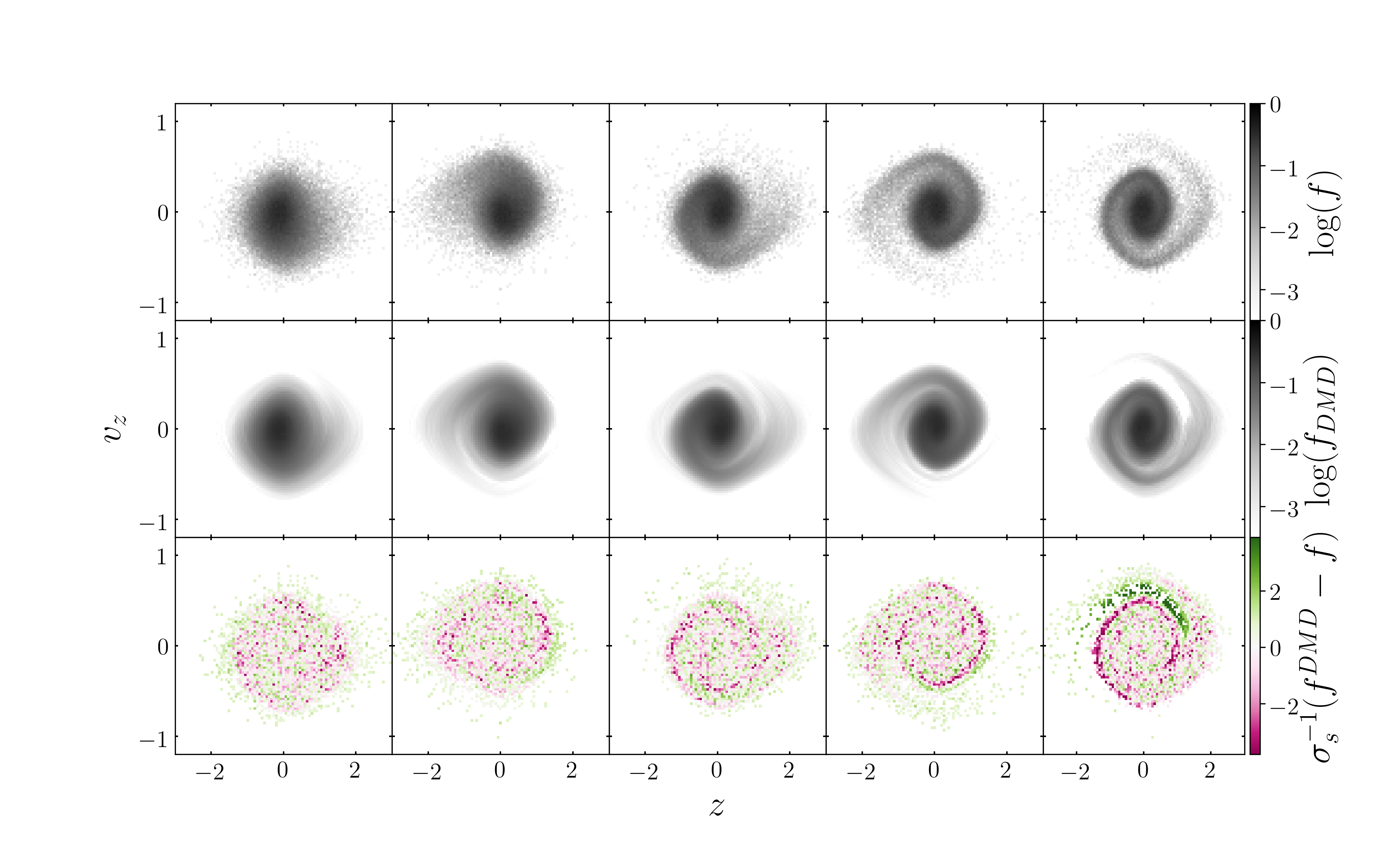
Figure 6: Comparison of the DMD solution and the simulation data with residuals for $\alpha=0.2$. The error is computed in the same way as in Fig. 1. The snapshots are the same of those in Fig 5.

The decompositions for each live fraction yield a zero frequency equilibrium mode, and several complex oscillatory modes. In what follows we focus only on the complex modes. In Figs. 7, 8, and 9 we show the three most dominant modes of the DF excluding the equilibrium mode, for the live fractions $\alpha=0.8,0.5,0.2$. As these are all complex modes, we show only one member of each conjugate pair. We include the real and imaginary components, as well as the time dependent complex amplitudes. As indicated by the phase difference in the amplitudes, the modes effectively oscillate between the real and imaginary components.

In general we obtain a combination of damped and un-damped modes. Un-damped and very weakly damped modes are dominant in the DMD solution. These dominant modes behave similarly to normal modes, and in some cases are the true modes (like in section 3). They persist on long time scales relative the dynamical time of the system. Strongly damped modes correspond to transient responses of the system and the subsequent decay due to phase mixing and Landau damping (Binney & Tremaine, 2008).

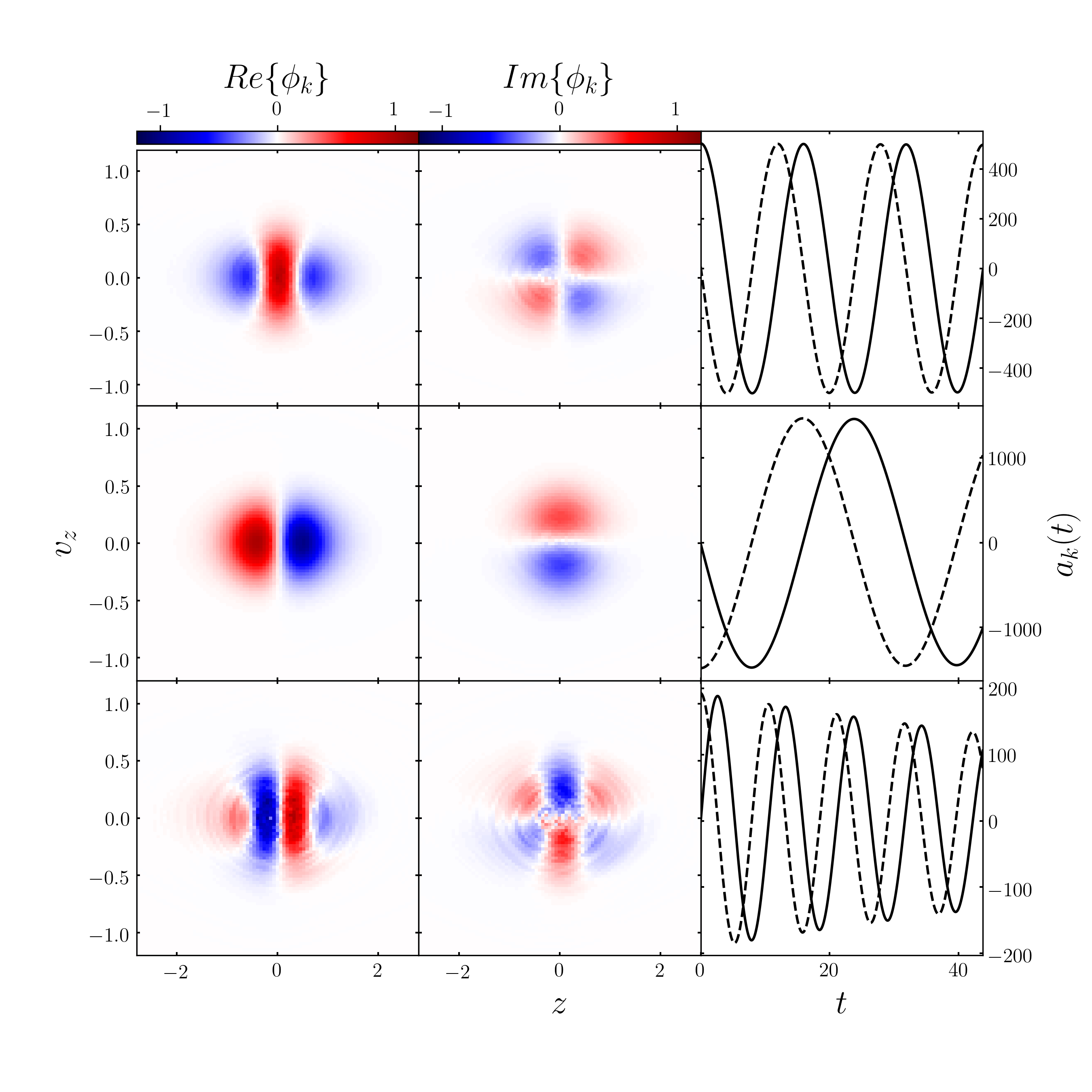
Figure 7: Three most dominant modes aside from the equilibrium mode for the case $\alpha=0.8$. In the right column, the solid and dashed curves correspond to the real and imaginary components of the amplitudes respectively. The modes are evaluated on the same grid used for the histograms in Fig. 5. The time axis in the third column is in units of $9.8$ Myr.

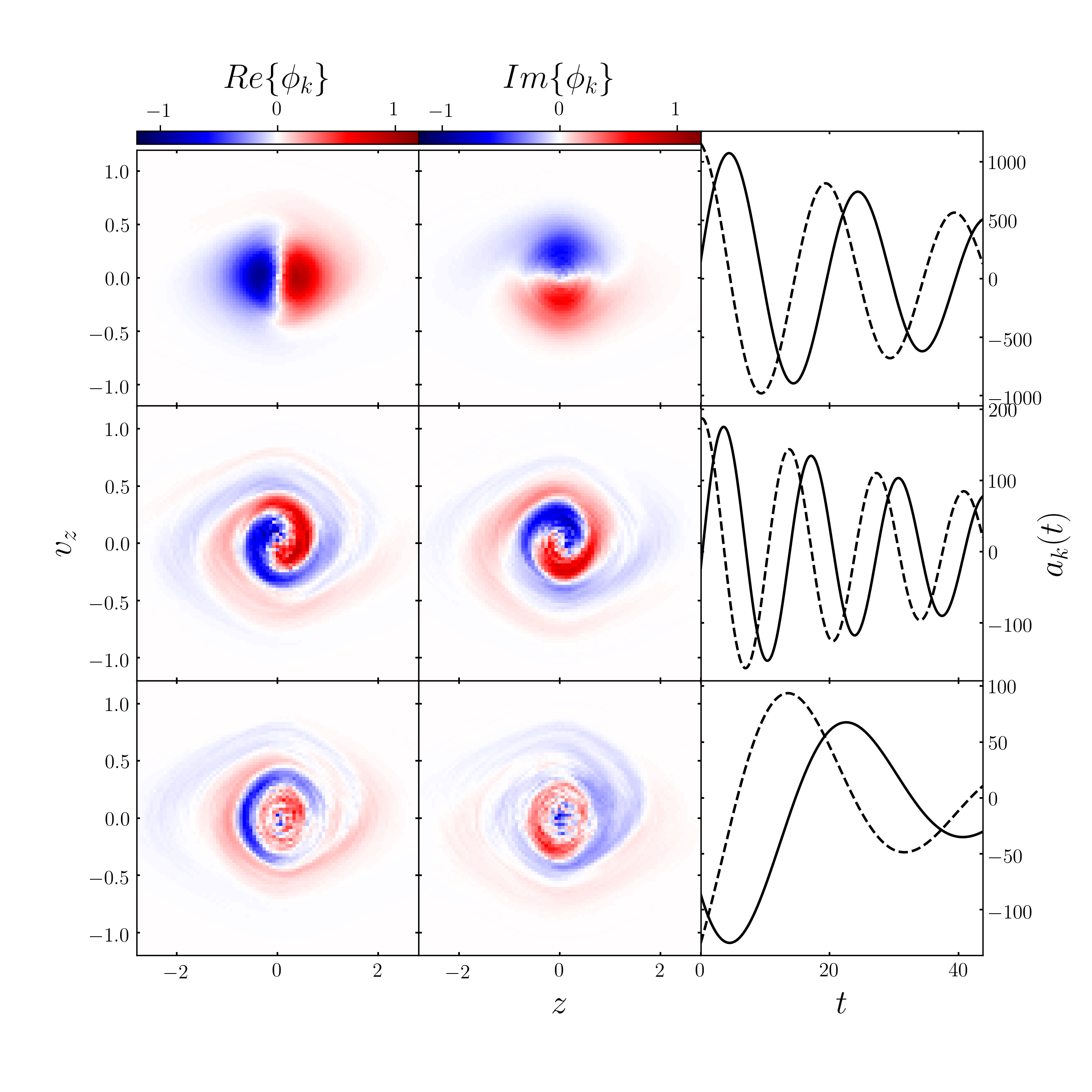
Figure 8: Same as figure 7 for $\alpha=0.5$

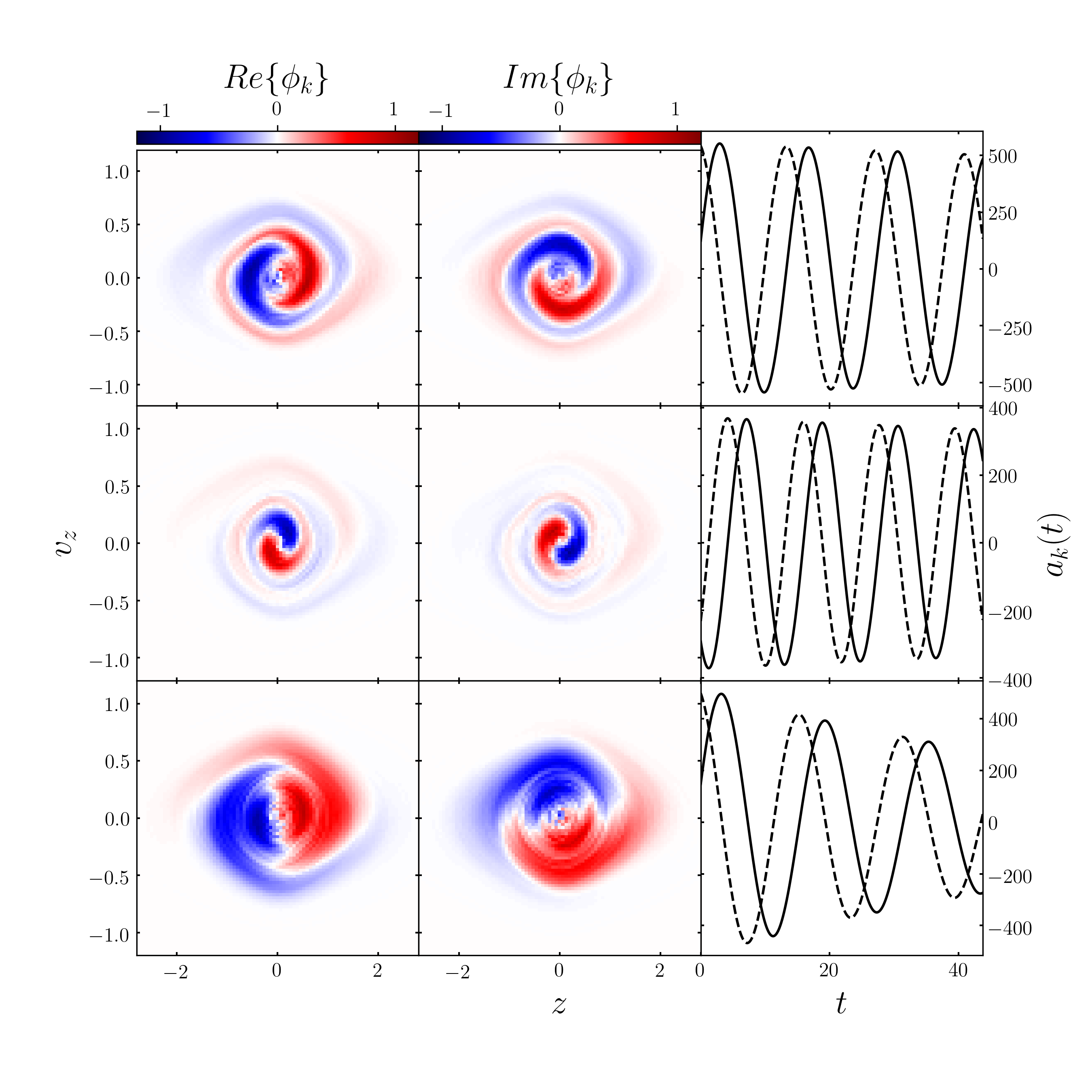
Figure 9: Same as figure 7 for $\alpha=0.2$

In addition to the mode structures, we can also make use of the corresponding eigenvalues in understanding the temporal behavior of the modes, and the dimensionality of the DMD solution. Recalling that the frequencies are related to the eigenvalues via $\omega_{j}=\ln{\lambda_{j}}/\Delta t$, and considering the eigenvalues in polar form, $\lambda=|\lambda|e^{i\theta_{\lambda}}$ one has that the frequencies can be written as

$$\omega=\tfrac{1}{\Delta t}\big{(}\ln|\lambda|+i\theta_{\lambda}\big{)}.$$ (32)

From equation 23, we see that $|\lambda|$ determines the growth or decay rate of each mode, while $\theta_{\lambda}$ sets the mode oscillation frequency. It is also convenient to define the mode lifetime

$$\tau=\frac{\Delta t}{\ln|\lambda|},$$ (33)

which we can compare to the orbital period of the system, $T$. We show in Fig. 10 the coordinate system in the complex plane that we will use to interpret the eigenvalues. This consists of curves of constant lifetime and frequency, indicating the physical meaning of an eigenvalue’s position in the complex plane. Modes with $|\lambda|\approx 1$ will persist, while modes with $|\lambda|<1$ will damp on the timescales indicated by the lifetime curves. Thus, the long term behavior of the system may be approximated by a sum over modes with eigenvalues near the unit circle. In Fig. 11 we show the eigenvalue spectra for each choice of $\alpha$ on the relevant patch of the plane in Fig. 10. In addition to mapping the modes to lifetime and frequency, these plots provide an indication of the dimensionality of the phase space structure in the DMD basis, as they show how many modes will persist through the time evolution of the system.

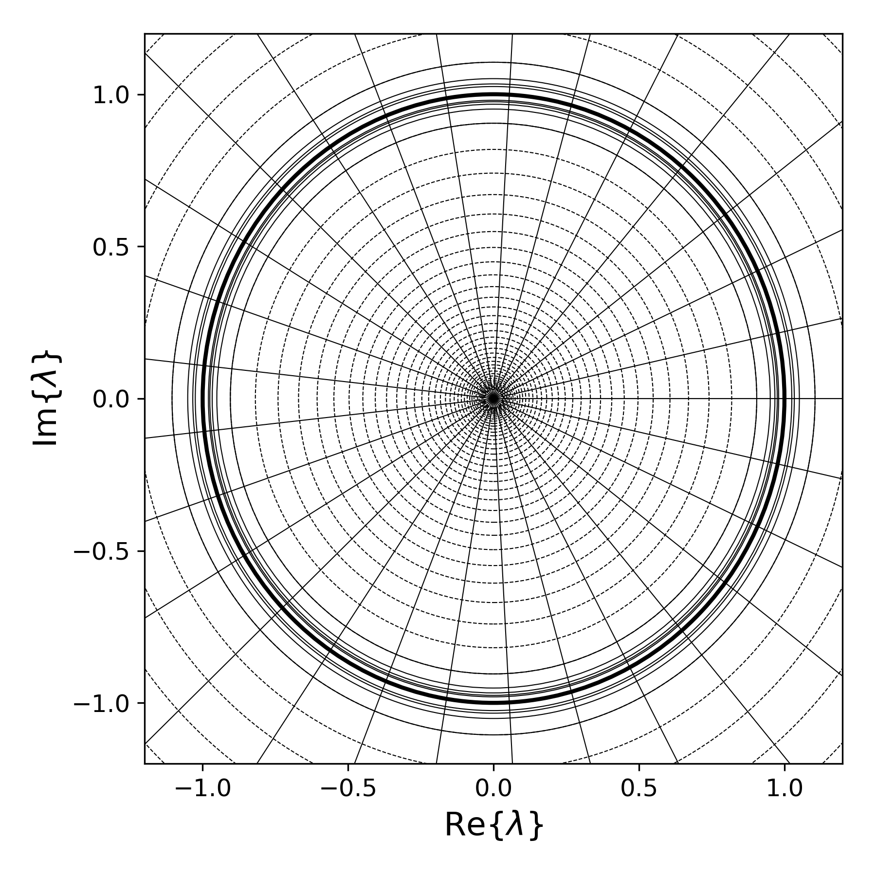
Figure 10: The coordinate system used to interpret the eigenvalues corresponding to the DMD modes. The radial lines are curves of constant mode frequency, increasing with absolute angle in the plane. The thick circle is the unit circle, and modes with eigenvalues lying on this curve do not grow or decay (true modes). Curves inside the unit circle are curves of constant lifetime for stable modes, with lifetime increasing as they move towards the unit circle. Curves outside the unit circle are curves of constant growth rate for unstable modes, with growth rate increasing as they move away from the unit circle. The solid curves are integer multiples of orbital period, while the dashed curves go as $\tau=T/s,\ s\in\mathbb{Z}$.

Figure 11: Eigenvalues plotted in the complex plane as described in Fig. 10. From left to right, the panels correspond to $\alpha=0.8,0.5,0.2$. The dashed curves here correspond to modes lifetimes of $T$, $2T$, $3T$ and $4T$ in that order as they approach the unit circle. There are six eigenvalues that are not shown in the $\alpha=0.8$, as they are well within the $\tau=T$ circle, and correspond to extremely rapidly damped modes that do not contribute to the dominant structure.

Note that in this discussion, we are concerned only with the dynamics present in the simulation. That is, we are using DMD as a diagnostic tool, not for future state prediction (see Kutz et al. (2016)). We do not then concern ourselves with the accuracy of the DMD solution outside of the time interval of the simulation.

4.3 Mode Interpretation

We now discuss the physical interpretation of the isothermal plane DMD modes, describing their possible connection to known normal modes in Section 4.3.1, and their relevance to phase mixing in Section 4.3.2.

4.3.1 Bending and Breathing Modes

In the case of $\alpha=0.8$, where self-gravity dominates the evolution over the external potential, the dominant modes in rows one and two of Fig. 7 share aspects of their morphology with breathing and bending modes derived in Mathur (1990) and Weinberg (1991) and further studied in Widrow et al. (2014) and Widrow & Bonner (2015). These modes are not damped, and have integer multiple frequencies. The sum of the conjugate pairs for each of these modes rotate clockwise in the $(z,v_{z})$ plane with a pattern speed set by the mode frequency, which is also consistent with theoretical models. However the modes in the first and second rows of Fig. 7 oscillate between the structures shown in the real and imaginary components, which differs from the Weinberg modes. The true modes of the isothermal plane are discrete, but lie very close to a continuum. As such they have proven difficult to excite in simulations (Weinberg, 1991). We believe that the modes we see here are mixtures of the true modes.

4.3.2 Phase Space Spirals

In the cases with moderate or weak self-gravity ($\alpha=0.5$ and $\alpha=0.2$, respectively) phase mixing becomes important and the DMD algorithm finds modes with spiral structure. As these spiral modes capture the structure in the DF we expect from phase mixing, one might think they are strictly a transient response. Although this is the case for many of the modes, there are un-damped persisting spiral modes, such as those in rows one and two of Fig. 9. Additionally, the mode in row one of Fig. 8, which is qualitatively similar to a bending mode, has a left-handed spiral structure apparent in both the real and imaginary components. Although we do not claim that there are true spiral modes, it is evident that the inclusion of self-gravity in a phase mixing system allows for persistent, dominant spiral modes. Consequently this means phase space spirals can persist on longer timescales than expected from pure kinematic phase mixing, as was argued in Darling & Widrow (2018).

The variation in mode structure and lifetime with live fraction indicates that self gravity and phase mixing can be thought of as competing effects, and there is a regime of relative strength of these effects in which spiral modes can persist on long timescales. We argue then that if the live fraction is in the appropriate regime, phase space spirals could be observed at a somewhat arbitrary time in the evolution of the system, independent of the timing expected from pure kinematic phase mixing. Under the assumption that stars in the solar neighborhood evolve according to their mutual interactions in the presence of an external potential, an estimated effective live fraction for this region of the Galaxy could yield an alternative estimate on the timing of GDR2 spirals than those made assuming only a background potential.

The result that a system undergoing phase mixing in the presence of self gravity can possess persisting spiral modes, in combination with the connection between perturbation theory and DMD demonstrated in Section 3, indicates that one may consider spiral modes as first order perturbations on the equilibrium distribution. With this, it would be possible to estimate the potential corresponding to perturbative spiral modes, which may be indicative of the form of perturbations that lead to phase space spirals like those observed in GDR2.

5 Extensions

Thus far we have focused on one-dimensional models. A logical next step is to apply DMD to full three dimensional simulations. The DMD algorithm itself is robust to very large data matrices. The challenge is to find an appropriate set of observables for each snapshot. In the one-dimensional case, we had the luxury of high particle resolution in the $(z,v_{z})$ phase space, and consequently could use a high grid resolution when evaluating $f(z,v_{z})$. In the case of full three-dimensional simulations, a simple binning procedure in 6D phase space is unfeasible for anything beyond the coarsest grid.

Suppose one is interested in using DMD to study the phase spirals found by Antoja et al. (2018) across the disc. One might imagine the following strategy: First sort particles in $N_{R}$ radial bins. For each bin, construct a Fourier series in Galactic azimuth, keeping only $N_{\phi}$ terms. Then, for each azimuthal mode number $m$ bin particles in an $N_{z}\times N_{v}$ grid across the $z-v_{z}$ plane. Finally, for each of the $N_{R}N_{\phi}N_{z}N_{v}$ cells, compute the first $m_{\rm max}$ moments of $v_{R}$ and $v_{\phi}$. For example, with $m_{\rm max}=2$ there are six moments. For $N_{R}=20$, $N_{\phi}=9$, $N_{z}=N_{v}=40$, and $m_{\rm max}=2$ we have approximately $1.7M$ cells, which would require a simulation with several hundred million particles, a large but feasible quantity.

On the other hand, if one is interested in spiral structure and warps, then an approach akin to the Fourier methods introduced by Sellwood & Athanassoula (1986) and extended to bending waves by Chequers et al. (2018) provide an attractive alternative. In this case, one computes the surface density and vertical moments of the DF, such as the mean midplane displacement and mean vertical velocity as functions of $R$ and $\phi$ across the disc. These quantities in a time series are then used to compose the DMD data matrices.

6 Conclusion

We have showed that DMD facilitates an analysis analogous to normal modes, with great generality in how it may be applied to problems in galactic dynamics. When applied to time series measurements of phase space density, DMD yields a finite series solution for the DF. The dominant terms in this series are typically un-damped or very weakly damped oscillations that can persist on long time scales relative to the orbital period. Moreover, the method can capture the physics of both phase mixing and self-gravity. By computing DMD modes, one can describe and study time-dependent phase space structure throughout its evolution in terms of a just a few eigenfunctions and their time-dependent coefficients. This provides a much richer look at the evolution of structure than typical spectral methods and allows analysis in terms of very few quantities compared to the full data set yielded by N-body simulations. The method should be even more powerful in the case of simulations of the complete 6D phase space.

We have observed how the competing effects of self gravity and phase mixing manifest in DMD modes. In the presence of both effects, persisting spiral modes arise. In the DMD solution, the spiral modes are responsible for the apparent phase mixing in the full DF. The eigenvalues associated with these modes should yield insight into the timescale of phase space spirals, and the structure of the eigenfunctions themselves can inform perturbations in the potential associated with non-equilibrium phenomena.

The observational evidence for a Galaxy in disequilibrium has led to a keen interest in the DF for the stellar disc and specifically the form and timescale of the perturbations. Since this is inherently a time-dependent problem, numerical studies are a key component in understanding the complete picture. DMD has the potential to provide valuable insight into stellar dynamics just as it has in the field of fluid dynamics.

References

- Antoja et al. (2018) Antoja T., et al., 2018, Nature, 561, 360
- Antonov (1971) Antonov V. A., 1971, Trudy Astronomicheskoj Observatorii Leningrad, 28, 64
- Arnold (1989) Arnold V. I., 1989, Mathematical Methods of Classical Mechanics. Springer-Verlag New York
- Bennett & Bovy (2018) Bennett M., Bovy J., 2018, MNRAS, 482, 1417
- Binney (1992) Binney J., 1992, ARA&A, 30, 51
- Binney & Tremaine (2008) Binney J., Tremaine S., 2008, Galactic Dynamics: Second Edition. Princeton University Press
- Binney et al. (1998) Binney J., Jiang I.-G., Dutta S., 1998, MNRAS, 297, 1237
- Bland-Hawthorn et al. (2019a) Bland-Hawthorn J., et al., 2019a, MNRAS, 486, 1167
- Bland-Hawthorn et al. (2019b) Bland-Hawthorn J., et al., 2019b, MNRAS, 486, 1167
- Camm (1950) Camm G. L., 1950, MNRAS, 110
- Carlin et al. (2013) Carlin J. L., et al., 2013, ApJ, 777, L5
- Chequers et al. (2018) Chequers M. H., Widrow L. M., Darling K., 2018, MNRAS, 480, 4244
- Cui et al. (2012) Cui X.-Q., et al., 2012, Research in Astronomy and Astrophysics, 12, 1197
- Darling & Widrow (2018) Darling K., Widrow L. M., 2018, MNRAS, 484, 1050
- Freeman (1978) Freeman K. C., 1978, in Berkhuijsen E. M., Wielebinski R., eds, IAU Symposium Vol. 77, Structure and Properties of Nearby Galaxies. pp 3–10
- Gaia Collaboration et al. (2018a) Gaia Collaboration et al., 2018a, A&A, 616, A1
- Gaia Collaboration et al. (2018b) Gaia Collaboration et al., 2018b, A&A, 616, A11
- Hunter & Toomre (1969) Hunter C., Toomre A., 1969, ApJ, 155, 747
- Kalnajs (1973) Kalnajs A. J., 1973, ApJ, 180, 1023
- Khoperskov et al. (2019) Khoperskov S., Di Matteo P., Gerhard O., Katz D., Haywood M., Combes F., Berczik P., Gomez A., 2019, A&A, 622, L6
- Kutz et al. (2016) Kutz J. N., Brunton S. L., Brunton B. W., Proctor J. L., 2016, Dynamic Mode Decomposition: Data-Driven Modeling of Complex Systems. SIAM
- Laporte et al. (2019) Laporte C. F. P., Minchev I., Johnston K. V., Gómez F. A., 2019, MNRAS, 485, 3134
- Leeuwin et al. (1993) Leeuwin F., Combes F., Binney J., 1993, Monthly Notices of the Royal Astronomical Society, 262, 1013
- Li & Shen (2019) Li Z.-Y., Shen J., 2019, arXiv e-prints,
- Mathur (1990) Mathur S. D., 1990, MNRAS, 243, 529
- Mezić (2005) Mezić I., 2005, Nonlinear Dynamics, 41, 309
- Press et al. (2002) Press W. H., Teukolsky S. A., Vetterling W. T., Flannery B. P., 2002, Numerical Recipes in C: The Art of Scientific Computing Second Edition. Cambrdige University Press
- Price-Whelan et al. (2015) Price-Whelan A. M., Johnston K. V., Sheffield A. A., Laporte C. F. P., Sesar B., 2015, MNRAS, 452, 676
- Quillen et al. (2018) Quillen A. C., et al., 2018, MNRAS, 480, 3132
- Rowley et al. (2009) Rowley C. W., Mezic I., Baghrti S., Schlatter P., Henningson D. S., 2009, Journal of Fluid Mechanics, 641, 115
- Schmid (2010) Schmid P. J., 2010, Journal of Fluid Mechanics, 656, 5
- Schönrich & Binney (2018) Schönrich R., Binney J., 2018, MNRAS, 481, 1501
- Sellwood (2013) Sellwood J. A., 2013, Dynamics of Disks and Warps. p. 923, doi:10.1007/978-94-007-5612-0_18
- Sellwood & Athanassoula (1986) Sellwood J. A., Athanassoula E., 1986, MNRAS, 221
- Sparke & Casertano (1988) Sparke L. S., Casertano S., 1988, MNRAS, 234, 873
- Spitzer (1942) Spitzer L., 1942, ApJ, 95
- Steinmetz et al. (2006) Steinmetz M., et al., 2006, AJ, 132, 1645
- Tremaine (1999) Tremaine S., 1999, MNRAS, 307, 877
- Tu et al. (2014) Tu J. H., Rowley C. W., Luchtenburg D. M., Brunton S. L., Kutz J. N., 2014, Journal of Computational Dynamics, 1, 391
- Weinberg (1991) Weinberg M. D., 1991, ApJ, 373, 391
- Widrow & Bonner (2015) Widrow L. M., Bonner G., 2015, MNRAS, 450, 266
- Widrow et al. (2012) Widrow L. M., Gardner S., Yanny B., Dodelson S., Chen H.-Y., 2012, ApJ, 750, L41
- Widrow et al. (2014) Widrow L. M., Barber J., Chequers M. H., Cheng E., 2014, MNRAS, 440, 1971
- Williams et al. (2013) Williams M. E. K., et al., 2013, MNRAS, 436, 101
- Xu et al. (2015) Xu Y., Newberg H. J., Carlin J. L., Liu C., Deng L., Li J., Schönrich R., Yanny B., 2015, ApJ, 801, 105
- Yanny & Gardner (2013) Yanny B., Gardner S., 2013, ApJ, 777, 91
- Yanny et al. (2009) Yanny B., et al., 2009, AJ, 137, 4377
- van der Kruit & Searle (1981) van der Kruit P. C., Searle L., 1981, A&A, 95, 105