The uniform general signed rank test and its design sensitivity

Abstract

A sensitivity analysis in an observational study tests whether the qualitative conclusions of an analysis would change if we were to allow for the possibility of limited bias due to confounding. The design sensitivity of a hypothesis test quantifies the asymptotic performance of the test in a sensitivity analysis against a particular alternative. We propose a new, non-asymptotic, distribution-free test, the uniform general signed rank test, for observational studies with paired data, and examine its performance under Rosenbaum’s sensitivity analysis model. Our test can be viewed as adaptively choosing from among a large underlying family of signed rank tests, and we show that the uniform test achieves design sensitivity equal to the maximum design sensitivity over the underlying family of signed rank tests. Our test thus achieves superior, and sometimes infinite, design sensitivity, indicating it will perform well in sensitivity analyses on large samples. We support this conclusion with simulations and a data example, showing that the advantages of our test extend to moderate sample sizes as well.

1 Introduction

In the empirical study of causal effects, the use of standard statistical hypothesis tests, along with their concomitant $p$-values and confidence intervals, accounts only for the uncertainty introduced by sampling variability. However, in an observational study where treatment assignment has not been randomized, hidden biases due to unobserved confounding can be much larger than sampling uncertainty. As such, standard hypothesis tests may fail to be convincing if they assume the study is free of hidden bias, as a randomized experiment would be. A sensitivity analysis addresses this problem by formally testing whether the qualitative conclusions of a standard procedure would change if hidden bias of a certain magnitude were present (Rosenbaum, 2002).

When an investigator plans to run a sensitivity analysis, the choice of test statistic may no longer hinge solely on traditional measures such as Pitman efficiency. In particular, an investigator may seek a test statistic which is least sensitive to hidden bias, and thereby most likely to successfully distinguish treatment effects from bias, rather than one which is most likely to detect treatment effects in the absence of hidden bias. Design sensitivity is one way to quantify this idea for a particular test statistic (Rosenbaum, 2004, 2010a). Design sensitivity complements Pitman efficiency and other conventional means of comparing tests.

Rosenbaum (2010b) shows that a test statistic which focuses on a strongly-affected subgroup may achieve superior design sensitivity, as compared to a statistic which uses all observations. Rosenbaum (2012) shows that a particular test, Noether’s test, has excellent design sensitivity but poor power against small effects. Rosenbaum then proposes an adaptive test in which the $p$-value is given by the minimum of two $p$-values from two competing test statistics, correcting for multiple testing by analyzing the joint distribution of these two test statistics. This adaptive test is shown to get some of the best of both worlds, in terms of good power in small samples as well as high design sensitivity. In fact, the adaptive test attains the maximum design sensitivity of its two component tests. Rosenbaum and Small (2017) similarly propose an adaptive test which chooses from the better of two test statistics, one focused on a subgroup and one examining the entire population, with correction for multiple testing.

In this paper we examine a different adaptive test for paired data, in which we may adaptively choose from a large, highly dependent family of test statistics. We control for multiple testing using a uniform concentration bound for the stochastic process formed by this family of test statistics. This permits adaptively choosing among as many test statistics as we have observations, while achieving non-asymptotic, distribution-free error control. Our theoretical results characterize how this test achieves excellent design sensitivity, which can be infinite against light-tailed alternatives—that is, no matter the strength of confounding, the test will reject with probability approaching one asymptotically. We are not aware of previous discussion of such behavior.

The structure of this paper is as follows. After summarizing Rosenbaum’s sensitivity analysis model in Section 2, we describe our test in Section 3, proving that it achieves the promised Type I error control in Theorem 1. We then characterize its design sensitivity with Theorems 2 and 3 of Section 4. Section 5 gives simulation results for a variety of fixed-sample and uniform tests under several light- and heavy-tailed alternatives. We outline the handling of tied data in Section 6, while in Section 7 we illustrate the performance of our tests on an observational dataset examining the link between fish consumption and mercury concentration in the blood. Section 8 concludes and offers some promising avenues for future work.

2 Background and notation

2.1 Rosenbaum’s sensitivity analysis model for paired data

We begin with a review of Rosenbaum’s sensitivity analysis model for paired data (Rosenbaum, 2002). We have $n$ pairs of subjects. The subjects in the $i$^th pair have control potential outcomes $R_{Cij}$, treatment potential outcomes $R_{Tij}$, and treatment indicators $Z_{ij}$ for $j=1,2$ and $i\in[n]$. Let $\mathcal{F}$ be the $\sigma$-field generated by all the potential outcomes $(R_{Cij},R_{Tij})_{i\in[n],j\in[2]}$.

A sensitivity analysis allows us to test whether a positive conclusion of our study—that is, a rejection of the null—holds up under the possibility of limited confounding. To operationalize this notion, for each $\Gamma\geq 1$ we define the sensitivity analysis null hypothesis $H_{0}(\Gamma)$, which asserts that

• $R_{Ti1}=R_{Ci1}$ and $R_{Ti2}=R_{Ci2}$ for all $i\in[n]$, i.e., Fisher’s sharp null, and

• conditional on $\mathcal{F}$, treatment assignments are independent between pairs, and the treatment probabilities within each pair are related by the following odds ratio bounds:

  $$\frac{1}{\Gamma}\leq\frac{\mathbb{P}\left(\left.Z_{i1}=1\,\right|\,\mathcal{F}\right)/\mathbb{P}\left(\left.Z_{i1}=0\,\right|\,\mathcal{F}\right)}{\mathbb{P}\left(\left.Z_{i2}=1\,\right|\,\mathcal{F}\right)/\mathbb{P}\left(\left.Z_{i2}=0\,\right|\,\mathcal{F}\right)}\leq\Gamma,\quad\text{for all }i\in[n].$$ (1)

At $\Gamma=1$, this specifies that, within each pair, both units have the same (conditional) probability of treatment. This is the standard assumption which leads to valid randomization inference in the absence of hidden bias (Rosenbaum, 2002, §3.2).

Write $R^{\textup{obs}}_{ij}\coloneqq Z_{ij}R_{Tij}+(1-Z_{ij})R_{Cij}$ for the observed outcomes and $Y_{i}=(Z_{i1}-Z_{i2})(R^{\textup{obs}}_{i1}-R^{\textup{obs}}_{i2})$ for the observed treated-minus-control difference in the $i$^th pair. Under $H_{0}(\Gamma)$ we know that $Y_{i}=\pm\lvert R_{Ci1}-R_{Ci2}\rvert$ and

$$\frac{1}{1+\Gamma}\leq\mathbb{P}\left(\left.Y_{i}>0\,\right|\,\mathcal{F},Z_{i1}+Z_{i2}=1\right)\leq\frac{\Gamma}{1+\Gamma},$$ (2)

where for simplicity we assume $\mathbb{P}(Y_{i}=0)=0$ for all $i$ throughout this paper. In words, $H_{0}(\Gamma)$ asserts that there is no effect of treatment for any individual, but the treatment probabilities may differ within a pair in ways we cannot observe. This difference in treatment probabilities could introduce hidden bias into our estimates of the effect of treatment, but the magnitude of such bias is limited by the sensitivity parameter $\Gamma$. Again, $\Gamma=1$ recovers the standard null hypothesis which assumes no hidden bias is present, in which case $\mathbb{P}\left(\left.Y_{i}>0\,\right|\,\mathcal{F},Z_{i1}+Z_{i2}=1\right)=1/2$. Throughout the rest of this paper, we implicitly condition on the event $\{Z_{i1}+Z_{i2}=1,\forall i\in[n]\}$, and omit it from the notation.

This sensitivity analysis model provides a method to conduct valid hypothesis tests under limited confounding, but leaves open the choice of test statistic. In order to judge the relative benefits of different test statistics, we perform a power calculation, comparing the power of various test statistics in a test of the sensitivity analysis null $H_{0}(\Gamma)$. As with all power calculations, we must choose a particular alternative hypothesis under which to compute power. We define a “favorable” alternative hypothesis $H_{1}(G)$ for a distribution $G$ over $\mathbb{R}$, motivated by the following scenario:

• $R_{Cij}$ is an independent draw from some distribution $F$, for each $i\in[n],j=1,2$,

• $R_{Tij}=R_{Cij}+\tau_{i}$ for all $i,j$, where $\tau_{i}\in\mathbb{R}$ is drawn from some fixed distribution for each $i\in[n]$, and is constant within each pair; and

• $\mathbb{P}\left(\left.Z_{i1}=1,Z_{i2}=0\,\right|\,\mathcal{F}\right)=\mathbb{P}\left(\left.Z_{i1}=0,Z_{i2}=1\,\right|\,\mathcal{F}\right)=1/2$, with treatment (conditionally) independent between pairs.

In words, there is a constant treatment effect within pairs and no hidden bias due to unequal treatment probabilities. The alternative hypothesis $H_{1}(G)$ is then characterized by the induced distribution $G$ of the i.i.d. pair differences $Y_{i}=(Z_{i1}-Z_{i2})(R_{Ci1}-R_{Ci2})+\tau_{i}$; because there is no hidden bias, the mean of this distribution (when the mean exists) is the average treatment effect $\mathbb{E}\tau_{i}$. In most cases, we consider $\tau_{i}\equiv\tau$ constant across pairs, so that $G$ is the distribution of $R-R^{\prime}+\tau$, where $R$ and $R^{\prime}$ are independent draws from $F$; this distribution is symmetric about $\tau$. We also consider a “rare effects” model in which $\tau_{i}$ is zero for most pairs and equal to some large value for a small proportion of pairs. In this case, $G$ is a mixture with most mass placed on some distribution symmetric about zero, and the remaining mass on a copy of the distribution shifted to the right.

Rosenbaum’s sensitivity analysis model is only one of many possible approaches. For some others, refer to Cornfield et al. (1923/2009); Gilbert et al. (2003); Robins et al. (2000); Yu and Gastwirth (2005). See also Fogarty and Small (2016) for the related problem of sensitivity analysis for multiple outcomes within Rosenbaum’s model.

2.2 Sensitivity analysis with general signed rank statistics

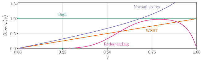
Figure 1: The four score functions $\varphi(q)$ used in this paper.

Let $(Y_{(i)})$ denote the pair differences $(Y_{i})$ ordered by absolute value, so that $\lvert Y_{(1)}\rvert\leq\lvert Y_{(2)}\rvert\leq\dots\leq\lvert Y_{(n)}\rvert$. A general signed rank statistic has the form

$$T_{n}=\sum_{i=1}^{n}\varphi\left(\frac{i}{n+1}\right)1_{Y_{(i)}>0}$$ (3)

for some score function $\varphi:(0,1)\to[0,\infty)$ (Lehmann and Romano, 2005; Rosenbaum, 2010b). The score function allows us to place more or less weight on pairs with larger or smaller observed absolute differences. We will consider four score functions in this paper, all illustrated in Figure 1:

• The sign test uses $\varphi(q)\equiv 1$, so that all pairs contribute equally, regardless of rank. In this case $T_{n}$ simply counts the number of pairs in which the treated unit had a higher outcome.

• The Wilcoxon signed rank test (WSRT) is equivalent to $\varphi(q)=q$ (Rosenbaum, 2010a), so that pairs with larger effects contribute more to the test statistic.

• The normal scores test uses $\varphi(q)=\Phi^{-1}((1+q)/2)$, where $\Phi^{-1}$ is the standard normal quantile function, $\mathbb{P}(Z\leq\Phi^{-1}(q))=q$ when $Z\sim\mathcal{N}(0,1)$. This score function is the quantile function of the absolute value of a standard normal random variable, and this general signed rank test has high power when outcomes are drawn from a normal distribution (Lehmann and Romano, 2005, §6.9-6.10).

• Finally, we include a “redescending” score function, $\varphi(q)=\sum_{l=\underline{m}}^{\overline{m}}\frac{l}{m}\binom{m}{l}q^{l-1}(1-q)^{m-l}$, so-called because this function rises as $q$ increases from zero, like the WSRT and normal scores functions do, but falls back to zero as $q$ approaches one, unlike the other three score functions. The resulting statistic puts more weight on pairs with larger absolute differences, but excludes the most extreme observations, which may be outliers. We set $(m,\underline{m},\overline{m})=(20,12,19)$. This score function approximates the $U$-statistic described in Rosenbaum (2011, Lemma 1), and the given values of $(m,\underline{m},\overline{m})$ were found to perform well in Rosenbaum’s study.

The sensitivity analysis null hypothesis $H_{0}(\Gamma)$ does not specify a single distribution for the observables $(Y_{i})$, but it does imply a single worst-case distribution for the test statistic $T_{n}$ in a one-sided test which rejects for $T_{n}$ sufficiently large—that is, a distribution which maximizes $\mathbb{P}\left(\left.T_{n}\geq a\,\right|\,\mathcal{F}\right)$ for any threshold $a$, among all distributions in $H_{0}(\Gamma)$. This worst-case distribution has the $n$ signs $(1_{Y_{i}>0})$ independent with $\mathbb{P}\left(\left.Y_{i}>0\,\right|\,\mathcal{F}\right)=\Gamma/(1+\Gamma)$ for all $i\in[n]$ (Rosenbaum, 2002, §4.3). Write $c_{\alpha,n}(\Gamma)$ for the $1-\alpha$ quantile of $T_{n}$ under this worst-case distribution, so that $c_{\alpha,n}(\Gamma)$ is the critical value of a one-sided, level-$\alpha$ sensitivity analysis testing $H_{0}(\Gamma)$ with test statistic $T_{n}$; the critical value may depend on $\mathcal{F}$, in the case of ties. This critical value yields a valid (conditional) test of the sensitivity analysis null hypothesis, and is not hard to approximate numerically or via the normal distribution. In Theorem 1 below, we build upon these ideas to define a uniform general signed rank test, deriving closed-form critical values which guarantee non-asymptotic Type I error control under the sensitivity null $H_{0}(\Gamma)$.

2.3 Power of a sensitivity analysis and design sensitivity

Under $H_{1}(G)$, the power of a one-sided, level-$\alpha$ sensitivity analysis for a general signed rank test with statistic $T_{n}$ is $\mathbb{P}_{1}(T_{n}\geq c_{\alpha,n}(\Gamma))$, which is well-defined since $H_{1}(G)$ specifies the distribution of $T_{n}$ completely. This power depends on the level $\alpha$, the sample size $n$, the sensitivity parameter $\Gamma$, the alternative distribution $G$, and the score function $\varphi$. The design sensitivity (Rosenbaum, 2004, 2010a) of the test statistic $T_{n}$ is the value $\widetilde{\Gamma}$ such that, as the sample size grows without bound, the power of a sensitivity analysis with parameter $\Gamma$ approaches one whenever $\Gamma<\widetilde{\Gamma}$ and approaches zero whenever $\Gamma>\widetilde{\Gamma}$:

$$\lim_{n\to\infty}\mathbb{P}_{1}(T_{n}\geq c_{\alpha,n}(\Gamma)) =1,\quad\text{for}\quad 1\leq\Gamma<\widetilde{\Gamma},\quad\text{and}$$ (4)

$$\lim_{n\to\infty}\mathbb{P}_{1}(T_{n}\geq c_{\alpha,n}(\Gamma)) =0,\quad\text{for}\quad\widetilde{\Gamma}<\Gamma<\infty.$$ (5)

Formally, the design sensitivity depends on the level $\alpha$, the alternative distribution $G$ and the score function $\varphi$. In typical examples, including those considered below, the dependence on $\alpha$ vanishes. It is clear from the definition that such a value is unique, if it exists, but existence must be proved as part of the derivation of design sensitivity, as in our Theorem 2. Note also that we may have $\widetilde{\Gamma}=\infty$, which means that $\lim_{n\to\infty}\mathbb{P}_{1}(T_{n}\geq c_{\alpha,n}(\Gamma))=1$ for all $\Gamma\geq 1$; in words, the test has power approaching one against the given alternative regardless of how large a sensitivity parameter $\Gamma$ is chosen.

Proposition 2 of Rosenbaum (2010b) gives a formula for the design sensitivity of a general signed rank test whenever the score function $\varphi$ is piecewise continuous, nondecreasing and not identically zero:

$$\widetilde{\Gamma}=\frac{\pi}{1-\pi},\quad\text{where}\quad\pi\coloneqq\frac{\int_{0}^{\infty}\varphi(G(y)-G(-y))\mathop{}\!\mathrm{d}G(y)}{\int_{0}^{1}\varphi(y)\mathop{}\!\mathrm{d}y}.$$ (6)

Note that $G(y)-G(-y)$ is the CDF of $\lvert Y\rvert$ under $H_{1}(G)$. We see that the design sensitivity of a general signed rank test is determined precisely by the aspects of $\varphi$ and $G$ captured in the quantity $\pi$. In Theorems 2 and 3, we extend this result to characterize the design sensitivity of our uniform general signed rank test. Our conditions on $\varphi$, while not strictly more general, do allow for the normal scores and redescending score functions, in contrast to Rosenbaum’s conditions.

For the sign test, $\varphi(q)\equiv 1$, we have $\int_{0}^{1}\varphi(y)\mathop{}\!\mathrm{d}y=1$ and $\int_{0}^{\infty}\varphi(G(y)-G(-y))\mathop{}\!\mathrm{d}G(y)$ is exactly $\mathbb{P}(Y>0)$ when $Y\sim G$. Hence $\pi=\mathbb{P}_{1}(Y>0)$ (cf. Rosenbaum, 2012, Proposition 1). In words, this $\pi$ is simply the probability that a pair difference $Y$ gives evidence in favor of a positive treatment effect, under the favorable alternative with no hidden bias.

3 A uniform general signed rank test

We now define a general class of uniform signed rank tests which operate on a family of related test statistics $(T_{n}(x))_{x\in(0,1)}$. Informally, our test rejects when any test statistic in the family lies above a corresponding modified critical value. These critical values are carefully chosen to correct for multiplicity by taking advantage of the structure of the family of test statistics. The uniform nature of our test yields advantages in terms of design sensitivity, which we describe in Section 4.

For any $\varphi:(0,1)\to[0,\infty)$, define the family of test statistics $(T_{n}(x))_{x\in(0,1)}$ by $T_{n}(x)=0$ for $x<1/(n+1)$, and for $x\geq 1/(n+1)$,

$$T_{n}(x)\coloneqq\sum_{i=\lceil(1-x)(n+1)\rceil}^{n}\varphi\left(\frac{i}{n+1}\right)1_{Y_{(i)}>0}=\sum_{i=\lceil(1-x)(n+1)\rceil}^{n}c_{i}1_{Y_{(i)}>0},$$ (7)

where we have defined $c_{i}\coloneqq\varphi\left(\frac{i}{n+1}\right)$ for convenience. For each $x$, $T_{n}(x)$ is a general signed rank statistic using the “truncated” score function $\varphi_{x}(q)=\varphi(q)1_{q\geq 1-x}$. There are $n$ distinct nontrivial test statistics in this family, $T_{n}(k/(n+1))$ for $k=1,\dots,n$, corresponding to the partial sums $\sum_{i=k}^{n}c_{i}1_{Y_{(i)}>0}$ for $k=n,n-1,\dots,1$. Hence the family corresponds to a random walk with $n$ steps and step sizes determined by the function $\varphi(\cdot)$.

Note that, despite the generality of our construction in terms of the score function $\varphi$, our family always consists of truncated versions of the full test statistic. Such truncated statistics focus on subsets of the experimental sample with large observed effects $\lvert Y_{i}\rvert$. As such, our test will tend to perform especially well against alternatives with large, rare effects.

Our uniform test will be characterized by a threshold function $f_{\alpha,n}(x)$, the uniform analogue of a critical value. Our test rejects whenever $T_{n}(x)\geq f_{\alpha,n}(x)$ for any $x\in(0,1)$. As in the fixed-sample case, there is a single worst-case distribution under $H_{0}(\Gamma)$ which maximizes the probability of rejection; we prove the following in Section A.1.

Proposition 1.

Fix any threshold function $f_{\alpha,n}:(0,1)\to\mathbb{R}_{>0}$. Among all distributions in $H_{0}(\Gamma)$, the rejection probability $\mathbb{P}\left(\left.\exists x\in(0,1):T_{n}(x)\geq f_{\alpha,n}(x)\,\right|\,\mathcal{F}\right)$ is maximized when $\mathbb{P}\left(\left.Y_{i}>0\,\right|\,\mathcal{F}\right)=\Gamma/(1+\Gamma)$ for all $i\in[n]$.

Under this worst-case distribution in $H_{0}(\Gamma)$, each step of the random walk equals $c_{i}$ with probability $\rho_{\Gamma}\coloneqq\Gamma/(1+\Gamma)$ and zero otherwise; these steps are independent. The resulting mean and variance of $T_{n}(x)$ are

$$\mu_{n}(x)\coloneqq\mathbb{E}T_{n}(x) =\rho_{\Gamma}\sum_{i=\lceil(1-x)(n+1)\rceil}^{n}c_{i}$$ (8)

$$\sigma_{n}^{2}(x)\coloneqq\operatorname{Var}T_{n}(x) =\rho_{\Gamma}(1-\rho_{\Gamma})\sum_{i=\lceil(1-x)(n+1)\rceil}^{n}c_{i}^{2}.$$ (9)

Our threshold function requires a tuning parameter $x_{0}>0$ to be fixed in advance, such that $\sigma_{n}^{2}(x_{0})>0$. If $\sigma_{n}^{2}(x)=0$ for all $x$, then we cannot choose a valid $x_{0}$, but in this case, $T_{n}(x)=0$ a.s. for all $x$, so we cannot reject for any reasonable bound. We then construct the following high-probability uniform upper boundary on the random walk $T_{n}(x)$:

$$f_{\alpha,n}(x)\coloneqq\frac{1}{\lambda_{n}}\left[\log\left(\frac{1}{\alpha}\right)+\sum_{i=\lceil(1-x)(n+1)\rceil}^{n}\log\left(1+\rho_{\Gamma}(e^{c_{i}\lambda_{n}}-1)\right)\right],\quad\text{where }\lambda_{n}\coloneqq\sqrt{\frac{2\log\alpha^{-1}}{\sigma_{n}^{2}(x_{0})}}.$$ (10)

For notational simplicity, we omit the dependence of $f_{\alpha,n}$ on $x_{0}$.

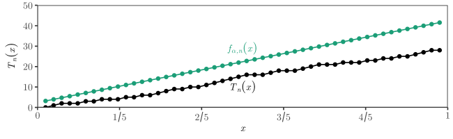
Figure 2: Illustration of Theorem 1 and the uniform bound (10) for the uniform sign test, $\varphi(q)\equiv 1$. Black line shows one realization of the random walk $T_{n}(x)$ for $x=1/(n+1),2/(n+1),\dots,n/(n+1)$; here $n=50$ and $\Gamma=2$. Green line shows the uniform upper bound $f_{\alpha,n}(x)$ which is unlikely to ever be crossed by the random walk. We may think of each value $f(1/(n+1)),f(2/(n+1)),\dots$ as a modified critical value for the corresponding test statistic.

Theorem 1.

Under $H_{0}(\Gamma)$, for any $x_{0}>0$ such that $\sigma_{n}^{2}(x_{0})>0$ and any $\alpha\in(0,1)$, we have

$$\mathbb{P}\left(\left.\exists x\in(0,1):T_{n}(x)\geq f_{\alpha,n}(x)\,\right|\,\mathcal{F}\right)\leq\alpha.$$ (11)

Theorem 1 justifies rejecting the sensitivity null $H_{0}(\Gamma)$ whenever $T_{n}(x)\geq f_{\alpha,n}(x)$ for some $x\in(0,1)$, allowing us to adaptively choose a value of $x$ after seeing the data, while retaining Type I error control at level $\alpha$. We call this test a uniform general signed rank test. The idea is illustrated in Figure 2. Because the probability bound in Theorem 1 holds uniformly over all $x$, in any given dataset we may choose the value of $x$ which yields the strongest inference. We can think of the resulting test as simultaneously conducting general signed rank tests with truncated score functions $\varphi_{x}(q)=\varphi(q)1_{q\geq 1-x}$ for all values $x=1/(n+1),\cdots,n/(n+1)$, but with modified critical values given by $f_{\alpha,n}(x)$. The critical value $f_{\alpha,n}(x)$ is larger than the fixed-sample exact critical value $c_{\alpha,n}(\Gamma)$ from Section 2.2, accounting for the uniformity of our test. Note that, when we use the sign test score function $\varphi(q)=1$, the resulting truncated score functions $\varphi_{x}$ are exactly the score functions used in Noether’s test (Noether, 1973; Rosenbaum, 2012).

Before proving Theorem 1 we give some intuition for the bound $f_{\alpha,n}$ based on the following asymptotic approximation, which holds under mild conditions on $\varphi$ as detailed in Section A.3:

$$f_{\alpha,n}(x)=\underbrace{\mu_{n}(x)+\left(1+\frac{\sigma_{n}^{2}(x)}{\sigma_{n}^{2}(x_{0})}\right)\sqrt{\frac{\sigma_{n}^{2}(x_{0})\log\alpha^{-1}}{2}}}_{g_{\alpha,n}(x)}+\mathcal{O}(1).$$ (12)

The leading term, $\mu_{n}(x)$, is $\mathcal{O}(n)$ and accounts for the drift of the random walk. The next term is $\mathcal{O}(\sqrt{n})$ and accounts for the deviations of the random walk about its mean. As discussed in Section A.3, the parameter $x_{0}$ determines the value of $x$ for which the boundary $g_{\alpha,n}(x)$ is optimized, and this motivates the choice of $\lambda_{n}$ in the definition of $f_{\alpha,n}$. Theorem 1 would continue to hold with any choice $\lambda_{n}>0$, but our choice yields the interpretable tuning parameter $x_{0}$.

The discussion in Section A.3 also shows that the remainder $g_{\alpha,n}(x)-f_{\alpha,n}(x)$ is always negative, so that $g_{\alpha,n}(x)$ yields an alternative threshold function with a simpler analytical form, but the resulting test has slightly less power. In fact, the uniform boundaries $f_{\alpha,n}$ and $g_{\alpha,n}$ are drawn from a broader framework for uniform concentration of random walks described in Howard et al. (2018a, b). Other boundaries are possible and will yield different performance; further exploration of alternative boundaries is a promising avenue of future work. We give below a short, self-contained proof of Theorem 1 to illustrate the techniques, which are closely related to the classical Cramér-Chernoff method (Cramér, 1938; Chernoff, 1952; Boucheron et al., 2013, section 2.2).

Proof of Theorem 1.

Throughout the proof, we condition on $\mathcal{F}$, dropping it from the notation for simplicity. Let $S_{i}\coloneqq 1_{Y_{(i)}>0}$ for $i\in[n]$, so that $T_{n}(k/(n+1))=\sum_{i=n+1-k}^{n}c_{i}S_{i}$ for each $k\in[n]$. By Proposition 1, under the worst-case distribution in $H_{0}(\Gamma)$, $(S_{i})_{i\in[n]}$ are distributed as $n$ i.i.d. $\operatorname{Bernoulli}(\rho_{\Gamma})$ random variables. The moment-generating function of the random variable $c_{i}S_{i}$ is

$$\mathbb{E}e^{\lambda c_{i}S_{i}}=1+\rho_{\Gamma}(e^{c_{i}\lambda}-1)\quad\forall\lambda\in\mathbb{R}.$$ (13)

Now define $(L_{k})_{k=0}^{n}$ by $L_{0}\coloneqq 1$ and, for $k\in[n]$,

$$L_{k} \coloneqq\exp\left\{\lambda_{n}T_{n}\left(\frac{k}{n+1}\right)-\sum_{i=n+1-k}^{n}\log\left(1+\rho_{\Gamma}(e^{c_{i}\lambda_{n}}-1)\right)\right\}=\prod_{i=n+1-k}^{n}\frac{e^{\lambda_{n}c_{i}S_{i}}}{1+\rho_{\Gamma}(e^{c_{i}\lambda_{n}}-1)}.$$ (14)

It is easy to see from (13) and (14) that $\mathbb{E}\left(\left.L_{k}\,\right|\,S_{n},S_{n-1},\dots,S_{n+2-k}\right)=L_{k-1}$, so that $L_{k}$ is a nonnegative martingale with respect to the natural filtration defined by the sequence $S_{n},S_{n-1},\dots,S_{1}$. Then Ville’s maximal inequality for nonnegative supermartingales (Ville, 1939; Durrett, 2013, Exercise 5.7.1) implies

$$\alpha \geq\mathbb{P}\left(\exists k\in[n]:L_{k}\geq\alpha^{-1}\right)$$ (15)

$$=\mathbb{P}\left(\exists k\in[n]:T_{n}\left(\frac{k}{n+1}\right)\geq f_{\alpha,n}\left(\frac{k}{n+1}\right)\right)$$ (16)

$$=\mathbb{P}\left(\exists x\in\left\{\frac{1}{n+1},\frac{2}{n+1},\ldots,\frac{n}{n+1}\right\}:T_{n}(x)\geq f_{\alpha,n}(x)\right)$$ (17)

$$=\mathbb{P}\left(\exists x\in(0,1):T_{n}(x)\geq f_{\alpha,n}(x)\right).$$ (18)

The final equality follows since the values $x=1/(n+1),2/(n+1),\dots,n/(n+1)$ capture all of the distinct values of both $T_{n}(x)$ and $f_{\alpha,n}(x)$ for $x\geq 1/(n+1)$, and adding the region $0<x<1/(n+1)$ does not change the overall probability since $T_{n}(x)=0$ over this region while $f_{\alpha,n}(x)$ is strictly positive. ∎

4 Design sensitivity of the uniform test

We have shown that the uniform test may be thought of as simultaneously conducting general signed rank tests at all values of $x$ with modified critical values $f_{\alpha,n}(x)$. We might equivalently think of this as adjusting the significance level $\alpha$ downwards, and to different values for different $x$, in computing critical values for a sequence of general signed rank tests. Recalling that the design sensitivity of a general signed rank test (6) does not depend on $\alpha$, we may wonder if the uniform test has design sensitivity equal to the maximum of the design sensitivities of the component test statistics $T_{n}(x)$. This conclusion is not quite trivial, since the “adjusted significance levels” in the uniform test vary as $n$ grows. Nonetheless, it turns out to be true. We prove this for score functions $\varphi:(0,1)\to[0,\infty)$ satisfying the following properties:

• $\int_{0}^{1}\varphi^{2}(x)\mathop{}\!\mathrm{d}x<\infty$;

• $\varphi$ is discontinuous on a set of Lebesgue measure zero;

• there exists a constant $a\in[0,1/2)$ such that $\varphi$ is nonincreasing on $(0,a)$, nondecreasing on $(1-a,1)$, and bounded on $(a,1-a)$; and

• $\int_{1-x}^{1}\varphi(x)\mathop{}\!\mathrm{d}x>0$ for all $x>0$.

Theorem 2.

Suppose $\varphi$ satisfies conditions (P1-P4) above, and $G$ is continuous. Then the design sensitivity of the corresponding uniform general signed rank test under $H_{1}(G)$ is

$$\widetilde{\Gamma}_{\varphi,{\textup{unif}}}\coloneqq\sup_{x\in(0,1)}\widetilde{\Gamma}(x)=\sup_{x\in(0,1)}\frac{\pi(x)}{1-\pi(x)},\quad\text{where}\quad\pi(x)\coloneqq\frac{\int_{0}^{\infty}\varphi(G(y)-G(-y))1_{G(y)-G(-y)\geq 1-x}\mathop{}\!\mathrm{d}G(y)}{\int_{1-x}^{1}\varphi(y)\mathop{}\!\mathrm{d}y}.$$ (19)

Most of the work in the proof of Theorem 2 is captured by the following pair of lemmas. The first, proved in Section A.3, characterizes the asymptotic behavior of the boundary $f_{\alpha,n}(x)$ as $n\to\infty$.

Lemma 1.

If $\varphi$ satisfies conditions (P1)-(P3) above, then for any $x_{0}>0$ such that $\sigma_{n}^{2}(x_{0})>0$, any $\alpha\in(0,1)$, and any $x\in(0,1)$, we have $n^{-1}\mu_{n}(x)\to\rho_{\Gamma}\int_{1-x}^{1}\varphi(y)\mathop{}\!\mathrm{d}y$ and $f_{\alpha,n}(x)=\mu_{n}(x)+\mathcal{O}(\sqrt{n})$ as $n\to\infty$.

The second lemma generalizes a result of Sen (1970); we give the proof in Section A.4.

Lemma 2.

If $\varphi$ satisfies conditions (P1-P3) above, and $Y_{1},Y_{2},\dots$ are drawn i.i.d. from a continuous distribution $G$, then

$$\lim_{n\to\infty}\frac{1}{n}\sum_{i=1}^{n}\varphi\left(\frac{i}{n+1}\right)1_{Y_{(i)}>0}=\int_{0}^{\infty}\varphi(G(y)-G(-y))\mathop{}\!\mathrm{d}G(y)\quad\text{a.s.}$$ (20)

Proof of Theorem 2.

Let $H(x)\coloneqq G(x)-G(-x)$ denote the distribution of $\lvert Y\rvert$. Fix any $x\in(0,1)$. Applying Lemma 2 to the truncated score function $\varphi_{x}(q)=\varphi(q)1_{q\geq 1-x}$ yields

$$\lim_{n\to\infty}\frac{T_{n}(x)}{n}=\int_{0}^{\infty}\varphi(H(y))1_{H(y)\geq 1-x}\mathop{}\!\mathrm{d}G(y)\quad\text{a.s.}$$ (21)

Meanwhile, Lemma 1 implies that

$$\lim_{n\to\infty}\frac{f_{\alpha,n}(x)}{n}=\rho_{\Gamma}\int_{1-x}^{1}\varphi(y)\mathop{}\!\mathrm{d}y.$$ (22)

Combining (22) with (21), we conclude that

$$\mathbb{P}(T_{n}(x)\geq f_{\alpha,n}(x))=\mathbb{P}(n^{-1}T_{n}(x)\geq n^{-1}f_{\alpha,n}(x))\to 1\\ \text{if }\int_{0}^{\infty}\varphi(H(y))1_{H(y)\geq 1-x}\mathop{}\!\mathrm{d}G(y)>\rho_{\Gamma}\int_{1-x}^{1}\varphi(y)\mathop{}\!\mathrm{d}y,$$ (23)

that is, if $\Gamma<\pi(x)/[1-\pi(x)]$. Since the uniform test rejects whenever $T_{n}(x)\geq f_{\alpha,n}(x)$ for some $x$, it will reject with probability approaching one whenever $\Gamma<\pi(x)/[1-\pi(x)]$ for some $x\in(0,1)$. By a similar argument, $\mathbb{P}(T_{n}(x)\geq f_{\alpha,n}(x))\to 0$ if $\Gamma>\pi(x)/[1-\pi(x)]$, so the uniform test will reject with probability approaching zero if $\Gamma>\pi(x)/[1-\pi(x)]$ for all $x\in(0,1)$. The conclusion follows. ∎

Compare Theorem 2 to Proposition 1 of Rosenbaum (2012). Rosenbaum constructs an adaptive test choosing between two test statistics and achieving design sensitivity equal to the maximum of the two component tests. Theorem 2 shows that this principle may be extended to an infinite family of tests, in this case because the family possesses a dependence structure that allows us to construct an appropriate uniform bound.

We note that all of the score functions introduced in Section 2.2 satisfy conditions (P1-P4). Most of these are obvious; the only work required is to show that the score function for the normal scores test satisfies property (P1), and we give the short proof in Section A.5.

Proposition 2.

For the normal scores function, $\varphi(q)=\Phi^{-1}((1+q)/2)$, we have $\int_{0}^{1}\varphi^{p}(x)\mathop{}\!\mathrm{d}x<\infty$ for all $p\geq 1$.

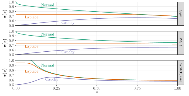
Figure 3: $\pi(x)$ from Theorem 2 for sign and WSRT score functions when $G$ is standard normal, Laplace (double exponential) or Cauchy. First two panels show alternative with $\tau=1/2$. Bottom panel shows rare effects model: 90% of pairs have no treatment effect, $\tau=0$ while 10% of pairs have a large treatment effect, $\tau=5$. See Figure 6 for corresponding plots with normal scores and redescending score functions, which have $\pi(x)$ qualitatively similar to that for the WSRT score function.

Figure 3 shows $\pi(x)$ as defined in Theorem 2. Each panel includes three alternative distributions $G$: normal with unit variance, Laplace (double exponential) with unit scale, and Cauchy with unit scale. In the first two panels, each distribution is centered at $\tau=1/2$. The bottom panel shows a “rare effects” model in which $G$ is a mixture of two of the given base distributions, one centered at zero receiving 90% of the total mass, and the other centered at $\tau=5$ receiving 10% of the total mass. This simulates a situation in which 90% of pairs have no treatment effect, while the remaining 10% of pairs have a large constant treatment effect, so that the average treatment effect remains equal to $1/2$.

The first two panels of Figure 3 show $\pi(x)$ for the sign and WSRT score functions introduced in Section 2.2; Section A.7 includes $\pi(x)$ plots for the normal scores and redescending score functions, which are qualitatively similar to $\pi(x)$ for the WSRT. For the sign test, $\pi(x)$ is maximized at some value $x<1$ under all distributions, although the increase is modest for the Laplace and Cauchy alternatives. This illustrates the benefits of truncation with the sign test. With the WSRT, we still see dramatic gains under a normal alternative, and indeed $\pi(x)\uparrow 1$ as $x\downarrow 0$ for all of our score functions under a normal alternative. This indicates we can achieve infinite design sensitivity under normal tails, a fact which we prove in Corollary 1. Under the Laplace or Cauchy alternatives, however, we do not see substantial gains in $\pi(x)$ as $x$ decreases from one for the WSRT; the same holds true for the normal scores and redescending score functions. Under the heavier-tailed Laplace and Cauchy alternatives, it seems, score functions which place more weight on larger outcomes do not benefit from narrowing attention to a subset of pairs with the largest absolute differences. Informally speaking, the higher likelihood of large outliers means less information is present in the tails.

The $\pi(x)$ functions in the bottom panel, computed under a rare effects model, tells a different story. Here, a uniform WSRT benefits from narrowing attention to a subset of pairs with large absolute differences regardless of the alternative distribution, although gains are still more modest for the Cauchy alternative than for the others. This confirms the intuitive fact that, when effects are large and rare, a test which restricts attention accordingly yields lower sensitivity to hidden bias.

Figure 3 makes it clear that the best choice of $x$ depends on the alternative distribution $G$ and the score function in a complicated manner. The advantage of our uniform test is that it can adapt to the alternative at hand without prior knowledge, achieving performance equivalent to the oracle choice of $x$ in terms of design sensitivity. It it also notable that all four score functions exhibit identical behavior near $x=0$. The following result makes this observation precise whenever $G$ is continuous with infinite support. We show that the limiting behavior of $\pi(x)$ as $x\downarrow 0$ is often determined by the tails of $G$ alone, not by the score function $\varphi$, and this may be used to lower bound the design sensitivity over a broad class of score functions.

Theorem 3.

Suppose $\varphi$ satisfies conditions (P1-P4) above, and suppose $G$ has positive density $g(x)$ with respect to Lebesgue measure for all $x\in\mathbb{R}$. Then

$$\widetilde{\Gamma}_{\varphi,{\textup{unif}}}\geq\liminf_{q\uparrow\infty}\frac{g(q)}{g(-q)}.$$ (24)

Proof.

Write $q_{x}$ for the $x$-quantile of $\lvert Y\rvert$ when $Y\sim G$, so that $q_{x}$ is defined by the equation $G(q_{x})-G(-q_{x})=x$. We shall require the derivative of $q_{x}$ below, which we find by implicit differentiation:

$$\frac{\mathop{}\!\mathrm{d}q_{x}}{\mathop{}\!\mathrm{d}x}=\frac{1}{g(q_{x})+g(-q_{x})}.$$ (25)

Now observe that, using the definition of $q_{x}$, we may write $\pi(x)$ from Theorem 2 as

$$\pi(x)=\frac{\int_{q_{1-x}}^{\infty}\varphi(G(y)-G(-y))\mathop{}\!\mathrm{d}G(y)}{\int_{1-x}^{1}\varphi(y)\mathop{}\!\mathrm{d}y}.$$ (26)

We apply the generalized form of L’Hôpital’s rule, which says that $\limsup f/g\geq\liminf f^{\prime}/g^{\prime}$ when $\lim f=\lim g=0$, to the formula (26) for $\pi(x)$ to find

$$\limsup_{x\downarrow 0}\pi(x) \geq\liminf_{x\downarrow 0}\frac{\frac{\mathop{}\!\mathrm{d}}{\mathop{}\!\mathrm{d}x}\int_{q_{1-x}}^{\infty}\varphi(G(y)-G(-y))\mathop{}\!\mathrm{d}G(y)}{\frac{\mathop{}\!\mathrm{d}}{\mathop{}\!\mathrm{d}x}\int_{1-x}^{1}\varphi(y)\mathop{}\!\mathrm{d}y}$$ (27)

$$=\liminf_{x\downarrow 0}\frac{\varphi(1-x)g(q_{1-x})}{\varphi(1-x)}\cdot\frac{1}{g(q_{1-x})+g(-q_{1-x})},$$ (28)

where the equality uses the fundamental theorem of calculus and (25). Condition (P4) on $\varphi$ implies $\varphi(q)$ must be positive on a neighborhood $q\in(1-\epsilon,1)$ for some $\epsilon>0$, which ensures the limit is well-defined. Reparametrizing in terms of $q=q_{1-x}$, and noting that $q_{1-x}\uparrow\infty$ as $x\downarrow 0$ since $g$ is positive throughout $\mathbb{R}$, we have

$$\limsup_{x\downarrow 0}\pi(x) \geq\liminf_{q\uparrow\infty}\frac{1}{1+\frac{g(-q)}{g(q)}}.$$ (29)

Hence $\limsup_{x\downarrow 0}\frac{\pi(x)}{1-\pi(x)}\geq\liminf_{q\uparrow\infty}\frac{g(q)}{g(-q)}$. The conclusion follows from Theorem 2. ∎

Plugging the normal density into Theorem 3 for $g(x)$ confirms the fact suggested by Figure 3:

Corollary 1.

If $G=\mathcal{N}(\tau,\sigma^{2})$, then $\widetilde{\Gamma}_{\varphi,{\textup{unif}}}=\infty$. That is, no matter what value of $\Gamma$ is used in a sensitivity analysis with a uniform general signed rank test, the power under $H_{1}(G)$ tends to one as $n\to\infty$.

5 Simulations

Figures 4 and 5 illustrate Theorem 2 with simulations under standard normal, Laplace and Cauchy alternatives; in each case $\tau=1/2$, except for the “rare effects” panels in Figure 4 which use the rare effects model described in Section 4. We simulate both standard, fixed-sample tests and uniform tests based on Theorem 1, with the four score functions introduced in Section 2.2. All tests are run with level $\alpha=0.05$ and plots are based on 10,000 replications.

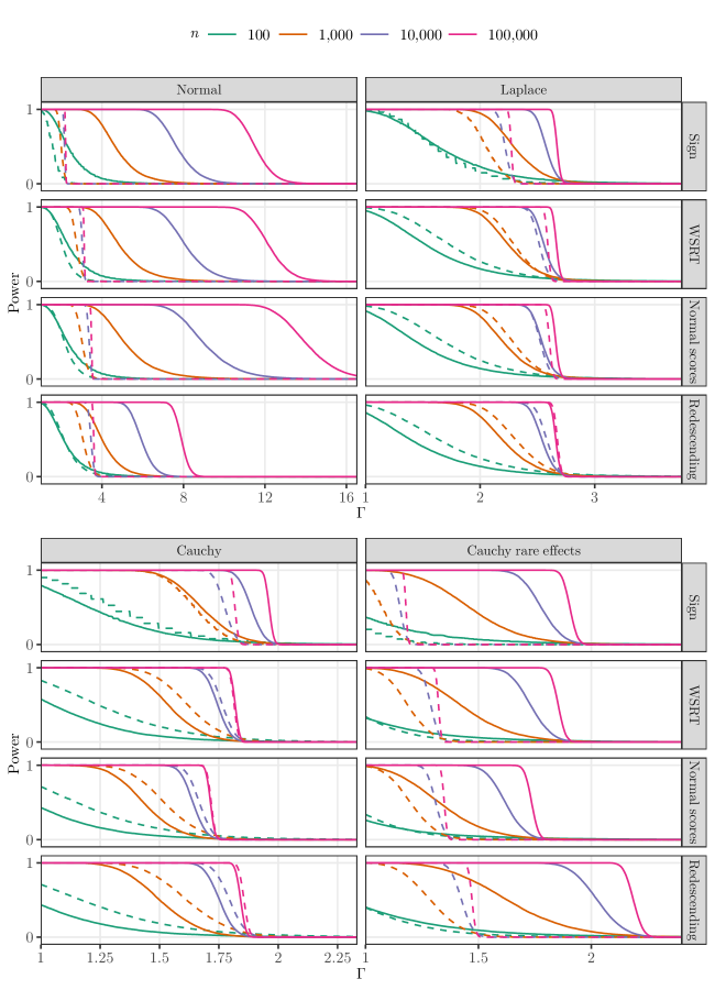
Figure 4: Comparison of simulated power for fixed-sample tests (dashed lines) vs. uniform tests (solid lines), based on 10,000 replications. “Cauchy rare effects” panels show “rare effects” alternative model based on Cauchy distribution, as described in Section 4. Other panels show alternative model $H_{1}(G)$ with distribution $G$ as indicated, having center $1/2$ and unit scale. All tests use $\alpha=0.05$.

The results are consistent with our findings above. Figure 4 compares power for each uniform test to the the corresponding fixed-sample test based on the same score function. In the normal case, the uniform test does not indicate finite design sensitivity, as we expect from Corollary 1, and all uniform tests show substantial gains over their fixed-sample counterparts for $n\geq$ 1,000. In the Laplace and Cauchy cases, the uniform sign test still shows gains, but uniform tests based on other score functions often fail to outperform their fixed-sample counterparts, as we expect from Figure 3. With large sample sizes, however, the uniform tests at least remain competitive in nearly all cases. Finally, the “rare effects” case again confirms our expectations from Figure 3, showing that each uniform test improves substantially on its fixed-sample counterpart, even with Cauchy noise. Though not shown, the gains for normal and Laplace noise under the rare effects model are even more dramatic, as one would expect by Figure 3.

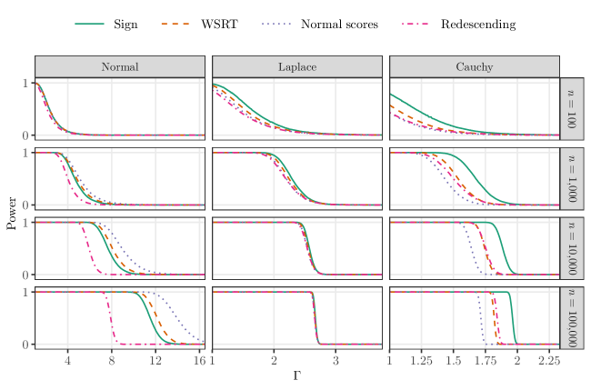
Figure 5: Comparison of simulated power for uniform tests using different score functions, based on 10,000 replications under alternative model $H_{1}(G)$ with $G$ as indicated, having center $1/2$ and unit scale. All tests use $\alpha=0.05$.

Figure 5 compares power between uniform tests with different score functions. Tests tend to perform similarly with small sample sizes, but clear distinctions emerge with large sample sizes. In the normal case, the normal scores test dominates while the redescending score function substantially underperforms. As we have seen, under normal noise the outliers contain the most information, and a score function which places more weight upon pairs with large absolute differences will attain higher power as a result. Conversely, in the Cauchy case, the normal scores tests performs the worst, while the sign test performs the best. Here the extreme tails yield less information, as indicated by Figure 3. The Laplace case is a middle ground in which the tails yield no more or less information than most of the rest of the distribution, as we have seen in Figure 3. Here the choice of score function makes little difference.

We close by noting that the uniform sign test shows considerable promise for use in practice. It is competitive in all cases and is the strongest performer of the four tests considered here in a number of cases. This is particularly interesting since the fixed-sample sign test is arguably the least attractive among the fixed-sample tests we have considered. It seems the landscape of uniform general signed rank tests is qualitatively different from that of their fixed-sample counterparts.

6 Handling ties

Under the assumption that outcomes are drawn from a continuous distribution, ties among outcome observations occur with probability zero. In practice however, tied outcome data may arise in a variety of settings. In this section we discuss how to adapt the results of the paper to the setting of ties.

Let $Y_{(1)},\ldots,Y_{(n)}$ be the outcome data ordered in any way so that $|Y_{(1)}|\leq|Y_{(2)}|\leq\ldots|Y_{(n)}|$. Note that this ordering is not unique when ties are present; in such cases, choose one such ordering arbitrarily. We may still apply the methods described in the paper directly to conduct a test. The test statistic and the uniform bound are clearly defined given our chosen ordering of outcomes, and Theorem 1 holds since no aspect of its proof depends on the absence of ties. We remark that it is reasonable to expect $\mathbb{P}(Y_{i}=0)>0$ in the presence of ties; however, this only reduces $\mathbb{P}\left(\left.Y_{i}>0\,\right|\,\mathcal{F}\right)$, so Proposition 1 and Theorem 1 continue to hold.

However, the version of our uniform test in Theorem 1 depends on the ordering we choose, perhaps arbitrarily, for $(Y_{(i)})$. To remove this undesirable feature of the procedure, we may instead use a generalization of $T_{n}(x)$ which is invariant to the specific choice of ordering in the tied setting. We write $T^{\star}_{n}(x)$ for this new test statistic. The intuition for $T^{\star}_{n}$ comes from recognizing that when ties are present, one or more test statistics in the family $(T_{n}(x))_{x\in(0,1)}$ are partial sums that include some terms with a particular absolute value but exclude others with the same absolute value, and that the scores associated with these terms may be different from one another. We obtain the family $(T^{\star}_{n}(x))_{x\in(0,1)}$ by replacing the score for each tied value by the average of scores for all indices involved in the tie, and by adding all these terms together to the partial sum rather than allowing partial sums that contain some terms but not all.

Formally, define $\mathcal{J}_{i}=\left\{j\in[n]:\ \left\lvert Y_{(j)}\right\rvert=\left\lvert Y_{(i)}\right\rvert\right\}$, the set of ranks with equal absolute pair differences to the $i$^th ranked pair. Let $m(i)=\min\mathcal{J}_{i}$, the lowest rank within the tied group containing the $i$^th ranked pair. Now define the test statistic

$$T^{\star}_{\varphi}(x)\coloneqq\sum_{\left\{i:m(i)\geq(1-x)(n+1)\right\}}c_{i}^{\star}1_{Y_{(i)}>0},\qquad\text{where}\qquad c_{i}^{\star}=\left\lvert\mathcal{J}_{i}\right\rvert^{-1}\sum_{j\in\mathcal{J}_{i}}\varphi\left(\frac{j}{n+1}\right).$$ (30)

When a group of pairs share the same absolute outcome value, this test statistic treats all these pairs as a single unit, including either all or none of them in the partial sum, and assigning each a score equal to the average score across all members in the tied set. Note that if there are only $k<n$ distinct absolute outcome values, there are only $k$ distinct nontrivial values for $T^{\star}_{n}(x)$; however, if no ties are present, $T^{\star}_{n}$ is identical to $T_{n}$.

We obtain a uniform boundary for $T^{\star}_{n}(x)$ by substituting $c^{\star}_{i}$ for $c_{i}$ in (9) and (10), yielding new quantities ${\sigma^{\star}_{n}}^{2}(x)$ and $f^{\star}_{\alpha,n}(x)$. In the absence of ties, the quantities ${\sigma^{\star}_{n}}^{2}$, and $f^{\star}_{\alpha,n}$ coincide with the original quantities $\sigma_{n}^{2}$, and $f_{\alpha,n}$. However, the quantities $(c_{i}^{\star})_{i=1}^{n}$ are random, unlike $(c_{i})$, hence $\sigma_{n}^{\star}$, and $f^{\star}_{\alpha,n}$ are random as well. This requires no real change to the analysis, since these quantities are $\mathcal{F}$-measurable and we condition on $\mathcal{F}$ throughout the proof of Theorem 1. As the reader may expect, the new boundary $f^{\star}_{\alpha,n}$ yields a valid uniform test of the sensitivity null $H_{0}(\Gamma)$ using the order-invariant test statistic $T_{n}^{\star}$.

Theorem 4.

Under $H_{0}(\Gamma)$, for any $\mathcal{F}$-measurable $x_{0}>0$ such that ${\sigma^{\star}_{n}}^{2}(x_{0})>0$ a.s., and any $\alpha\in(0,1)$, we have $\mathbb{P}\left(\left.\exists x\in(0,1):T^{\star}_{n}(x)\geq f^{\star}_{\alpha,n}(x)\,\right|\,\mathcal{F}\right)\leq\alpha$.

Proof.

Write $\widetilde{T}_{n}(x)\coloneqq\sum_{i=\lceil(1-x)(n+1)\rceil}^{n}c^{\star}_{i}1_{Y_{(i)}>0}$; this is the same as $T_{n}(x)$ with $c^{\star}_{i}$ substituted for $c_{i}$. Repeating the proof of Theorem 1 with $\sigma^{\star}_{n}$ and $f^{\star}_{\alpha,n}$ in place of their unstarred counterparts, we obtain

$$\mathbb{P}\left(\left.\exists x\in(0,1):\widetilde{T}_{n}(x)\geq f^{\star}_{\alpha,n}(x)\,\right|\,\mathcal{F}\right)\leq\alpha.$$ (31)

Since $m(i)\leq i$ and $c_{i}\geq 0$ for all $i$, we have $T^{\star}_{n}(x)\leq\widetilde{T}_{n}(x)$ for all $x$, which implies the result together with (31). ∎

7 Application: impact of fish consumption on mercury concentration

Mercury can be harmful to human health when concentrated too heavily in the bloodstream. There is a substantial body of evidence that consuming large amounts of fish can lead to elevated levels of mercury in the blood (Mahaffey et al., 2004). To study the impact of a high-fish diet on mercury concentration in the blood, we use data from the National Health and Nutrition Examination Survey or NHANES (Centers for Disease Control and Prevention National Center for Health Statistics (NCHS)(2017), CDC), which records detailed information about respondents’ diets and also contains analysis of blood samples, including a measure of total mercury concentration. We identified all 1,672 NHANES respondents from 2007 to 2016 who consumed an average of 15 or more servings of fish monthly, and matched each one to a similar respondent who consumed two or fewer servings of fish per month. Respondents were matched only to respondents from the same two-year period (2007-2008, 2009-2010, etc.). Within these groups, pairs were chosen by optimal matching with respect to a robust Mahalanobis distance (Rosenbaum, 2010a, sec. 8.3) computed from respondent age, household income, gender, ethnicity, cigarettes smoked per day, and indicators for high school graduation, missing high school graduation status, and smoking more than 7 cigarettes per day. Matches were also required to obey a propensity score caliper of 0.2 standard deviations based on a propensity score fitted to these same variables (Rosenbaum and Rubin, 1985). The final matched sample of 1,672 pairs achieved a high degree of balance on covariates, as shown in Table 1. Matching was conducted using R packages rcbalance and optmatch with package cobalt used for balance checking (Pimentel, 2016; Hansen and Klopfer, 2006; Greifer, 2018). For more discussion on the optimal construction of matched samples see Rosenbaum (1989), Hansen (2004), Zubizarreta et al. (2014), and Pimentel et al. (2015).

	Average attribute values		Standardized
Variable	15+ fish servings / mo	0-2 fish servings / mo	difference
Age	43.73	43.63	0.005
Household Income/(2x poverty line)	2.99	2.96	0.017
Female	0.46	0.46	0.004
Hispanic	0.19	0.18	0.002
Black	0.22	0.22	0.001
Smoker	0.44	0.42	0.011
Cigarettes/Day	4.09	4.04	0.011
High School Graduate	0.80	0.80	0.000
Missing HS Graduation Status	0.03	0.03	0.000

Table 1: Balance table for 1,672 matched pairs formed from NHANES data. Each pair contains one individual who consumed $\geq$15 servings of fish in the previous month, and one who consumed no more than two. The first two columns give the sample means in the matched samples for various attributes of interest, and the third gives the standardized difference, which is computed by dividing the difference in group sample means by the pooled standard deviation estimate from the full dataset before matching.

Note that although the balance on observed variables in Table 1 is very close, individuals with high-fish diets may differ from individuals with low-fish diets on many unobserved attributes correlated with mercury levels. Accordingly, we are interested not only in whether a test assuming an absence of unobserved confounders rejects the null hypothesis, but in how sensitive such a result is to potential bias from unobserved confounders.

In each of the 1,672 pairs formed, we computed the difference in total mercury concentration (in micrograms per mole) between the respondent with the high-fish diet and the respondent with the low-fish diet. The average concentration for matched individuals with high-fish diets and low-fish diets were 3.76 and 1.02 respectively, yielding an average pair difference of 2.73 micrograms per mole. We next tested the sharp null of no effect of treatment in any pair. Mercury measurements were rounded to two decimal places which led to some ties, so for each test we used the test statistic $T^{\star}_{n}(x)$ of Section 6 and $x_{0}=1/3$ in Theorem 4.

The first three columns of Table 2 show the results of sensitivity analysis in the matched data for the four general signed rank tests considered in this paper. For each of these test statistics, the naïve test with $\Gamma=1$ produces results highly significant at the 0.05 level, and the numbers in the table describe the smallest amount of unmeasured bias necessary to explain the observed effects assuming there is no true effect of treatment—that is, the minimum value of $\Gamma$ at which we fail to reject the sensitivity analysis null. For example, the fixed-sample sign test ceases to reject the null when we allow for an unobserved confounder which increases the odds of a high-fish diet by a factor of $\Gamma=4.82$; in contrast, the uniform sign test requires an unobserved confounder which increases the odds of a high fish diet by $\Gamma=10.51$ before it ceases to reject.

	1,672 pairs		190 pairs
Score function	Fixed-sample	Uniform	Fixed-sample	Uniform
Sign	4.82	10.51	3.72	8.29
Wilcoxon Signed Rank	8.06	10.47	6.04	8.09
Normal Scores	8.55	10.36	6.52	7.95
Redescending	9.68	9.97	7.26	7.58

Table 2: Sensitivity analysis for matched data. Each cell of the table represents a different test statistic for testing the null of no effect of a fish diet on mercury concentration; the first two columns give results for the full matched sample of 1,672 pairs, while the third and fourth columns give results for the smaller sample from 2015-2016 alone. The number in each cell is the smallest degree of unmeasured confounding $\Gamma$ necessary in the sensitivity analysis model before the test no longer rejects at the $\alpha=0.05$ level.

Note that repeating the same test many times with different test statistics, as in Table 2, is not recommended in practice. To avoid issues with multiple testing and Type I error control, one should select a single test statistic in advance, possibly based on a pilot sample as described in Heller et al. (2009). We show the results of several tests here to illustrate the impact of the choice of test statistic and complement the discussion in Section 5.

Several interesting patterns are clear in the full-sample results of Table 2. First, regardless of the score function used, the uniform version of the test is less sensitive to unmeasured bias than the fixed-sample version. This pattern is consistent with Theorem 2, which tells us that in large samples the uniform test should perform at least as well as any fixed-sample test it incorporates. Second, the performance of the uniform test across score functions varies much less than the performance of the fixed-sample version across score functions. In particular, the sign test performs substantially worse than any other test examined in the fixed-sample case, but it is comparable to (and even slightly better than) the other score functions in the uniform setting, corroborating the evidence from simulations in Section 5. In this dataset, as in the simulations, adapting over many different truncated statistics appears to compensate for the deficiencies of the fixed-sample sign test.

Finally, we briefly consider the importance of sample size by analyzing the subset of the matched dataset consisting only of those respondents from the final two-year period (2015-2016), a total of 190 pairs. The final two columns of Table 2 repeat the analysis for this smaller dataset. The same pattern of results is observed, with the uniform test outperforming the fixed-sample test for each score function, and the sign test performing best among uniform tests. Although the benefits of uniform testing articulated in Theorem 2 relate to asymptotic performance in large samples, uniform tests may also offer substantial improvement in datasets of only moderate size.

8 Conclusion and future work

We have described a new test for causal effects in a paired observational study, the uniform general signed rank test. This test provides non-asymptotically valid inference under Rosenbaum’s sensitivity analysis model and yields qualitative improvements in design sensitivity relative to existing methods. Our simulation results indicate that the advantages of this test extend from the asymptotic regime down to moderate sample sizes under a variety of alternative hypotheses, as well as to real-world studies.

Though we have described a sensible method for handling ties, we have focused our study on continuous outcomes. When ties are present but rare, as in the data example of Section 7, our findings should continue to hold. However, the study of outcomes with relatively few unique values may require alternative methodology. In such cases, the random walk $(T_{n}^{\star}(x))_{x\in(0,1)}$ will have relatively few steps, at most the number of unique values of the outcome, with each step comprised of many individual observations, namely all those pairs with absolute outcome equal to a given value. In the sequential analysis literature, such random walks are handled well by group sequential designs (Pocock, 1977; O’Brien and Fleming, 1979; Lan and DeMets, 1983; Jennison and Turnbull, 2000). An application to uniform general signed rank tests may yield promising future results.

Another interesting avenue is the evaluation other theoretical properties, beyond design sensitivity, of uniform general signed rank tests. For example, Lehmann and Romano (2005, Chapter 6) discuss the locally most powerful property of general signed rank tests against particular families of alternatives determined by the function $\varphi$. The uniform test is adaptively choosing from among a family of related $\varphi$ functions, and it would be interesting to understand what the implications are for local optimality in the sense discussed by Lehmann and Romano.

9 Acknowledgments

We thank Eli Ben-Michael for the conversation which sparked this project. Howard thanks Office Of Naval Research (ONR) Grant N00014-15-1-2367.

Appendix A Additional proofs

A.1 Proof of Proposition 1

Throughout the proof, we condition on $\mathcal{F}$, dropping it from the notation for simplicity. For each $i\in[n]$, write $S_{i}\coloneqq 1_{Y_{(i)}>0}$, $X_{i}\coloneqq T_{n}(i/(n+1))=\sum_{j=n-i+1}^{n}c_{j}S_{j}$, and $a_{i}\coloneqq f_{\alpha,n}(i/(n+1))$. Under $H_{0}(\Gamma)$, the $(S_{i})$ are independent with $1/(1+\Gamma)\leq\mathbb{P}(S_{i}=1)\leq\Gamma/(1+\Gamma)$. Let $p_{i}\coloneqq\mathbb{P}(S_{i}=1)$. We wish to show that the rejection probability $\mathbb{P}(\exists i\in[n]:X_{i}\geq a_{i})$ is maximized when $p_{i}=\Gamma/(1+\Gamma)$ for all $i\in[n]$.

Write $S\coloneqq(S_{1},\dots,S_{n})^{T}$, a random vector in $\{0,1\}^{n}$. Note that, for $s\in\{0,1\}^{n}$, $\mathbb{P}(S=s)=\prod_{i=1}^{n}p_{i}^{s_{i}}(1-p_{i})^{1-s_{i}}$. Let $\mathcal{R}\coloneqq\left\{s\in\{0,1\}^{n}:\sum_{j=n-i+1}^{n}c_{j}s_{j}\geq a_{i}\text{ for some }i\in[n]\right\}$. This set represents the rejection event, in the sense that the test rejects if and only if $S\in\mathcal{R}$. We will show that $\mathbb{P}(S\in\mathcal{R})$ is increasing in $p_{i}$ for each $i\in[n]$, from which it follows that the rejection probability is maximized when $p_{i}$ is maximized for each $i$.

We claim that if $s\in\mathcal{R}$ and $s^{\prime}\geq s$ elementwise, then $s^{\prime}\in\mathcal{R}$. To see this, observe that $s\in\mathcal{R}$ implies that we can choose $i\in[n]$ such that $\sum_{j=n-i+1}^{n}c_{j}s_{j}\geq a_{i}$. Then $\sum_{j=n-i+1}^{n}c_{j}s_{j}^{\prime}\geq\sum_{j=n-i+1}^{n}c_{j}s_{j}\geq a_{i}$, so $s^{\prime}\in\mathcal{R}$.

Now write $\mathbb{P}(S\in\mathcal{R})=\sum_{s\in\mathcal{R}}\prod_{i=1}^{n}p_{i}^{s_{i}}(1-p_{i})^{1-s_{i}}$, and differentiate with respect to $p_{k}$ for any $k\in[n]$:

$$\frac{\mathop{}\!\mathrm{d}}{\mathop{}\!\mathrm{d}p_{k}}\mathbb{P}(S\in\mathcal{R}) =\sum_{s\in\mathcal{R}}\left[(2s_{k}-1)\prod_{i\neq k}p_{i}^{s_{i}}(1-p_{i})^{1-s_{i}}\right]$$ (32)

$$=\sum_{\begin{subarray}{c}s\in\mathcal{R}\\ s_{k}=1\end{subarray}}\pi^{(k)}(s)-\sum_{\begin{subarray}{c}s\in\mathcal{R}\\ s_{k}=0\end{subarray}}\pi^{(k)}(s),$$ (33)

where $\pi^{(k)}(s)=\prod_{i\neq k}p_{i}^{s_{i}}(1-p_{i})^{1-s_{i}}$. For each $s\in\mathcal{R}$ with $s_{k}=0$, there corresponds an $s^{\prime}$ which is identical except for $s^{\prime}_{k}=1$, i.e., $s^{\prime}_{i}=s_{i}1_{i\neq k}+1_{i=k}$, and this $s^{\prime}\in\mathcal{R}$ by the claim above. Also, $\pi^{(k)}(s)=\pi^{(k)}(s^{\prime})$. Hence each term in the second sum of (33) is canceled by a term in the first sum. We conclude $\frac{\mathop{}\!\mathrm{d}}{\mathop{}\!\mathrm{d}p_{k}}\mathbb{P}(S\in\mathcal{R})\geq 0$, as desired. ∎

We remark that an alternative proof could use Holley’s inequality for distributions over finite distributive lattices (Rosenbaum, 2002, Sections 2.10, 4.7.2). We have opted for the direct proof above to keep the paper more self-contained.

A.2 A technical result on Riemann sums

The following result ensures convergence of certain Riemann sums for some unbounded functions, and is necessary to analyze the asymptotic behavior of $f_{\alpha,n}$.

Lemma 3.

Suppose $\varphi:(0,1)\to[0,\infty)$ is discontinuous on a set of measure zero, $\int_{0}^{1}\varphi(x)\mathop{}\!\mathrm{d}x<\infty$, and there exists a constant $a\in[0,1/2)$ such that $\varphi$ is nonincreasing on $(0,a)$, nondecreasing on $(1-a,1)$, and bounded on $(a,1-a)$. Then

$$\lim_{n\to\infty}\frac{1}{n}\sum_{i=1}^{n}\varphi\left(\frac{i}{n+1}\right)=\int_{0}^{1}\varphi(x)\mathop{}\!\mathrm{d}x.$$ (34)

Proof.

Write $\varphi=\varphi_{1}+\varphi_{2}+\varphi_{3}$ where $\varphi_{1}(x)\coloneqq\varphi(x)1_{x<a}$, $\varphi_{2}(x)\coloneqq\varphi(x)1_{a\leq x\leq 1-a}$, and $\varphi_{3}(x)\coloneqq\varphi(x)1_{x>a}$. Since $\varphi_{2}$ is bounded, it is Riemann integrable, so $n^{-1}\sum_{i=1}^{n}\varphi_{2}(i/(n+1))\to\int_{0}^{1}\varphi_{2}(x)\mathop{}\!\mathrm{d}x$ by standard Riemann integration theory, noting that $i/(n+1)\in((i-1)/n,i/n)$ for each $i\in[n]$. For $\varphi_{1}$ and $\varphi_{3}$, we appeal to Lemma 4 below to conclude that $n^{-1}\sum_{i=1}^{n}\varphi_{k}(i/(n+1))\to\int_{0}^{1}\varphi_{k}(x)\mathop{}\!\mathrm{d}x$ for $k=1,3$. The result follows by linearity. ∎

Lemma 4.

Suppose $\varphi:(0,1)\to[0,\infty)$ is monotone and $\int_{0}^{1}\varphi(x)\mathop{}\!\mathrm{d}x<\infty$. Then

$$\lim_{n\to\infty}\frac{1}{n}\sum_{i=1}^{n}\varphi\left(\frac{i}{n+1}\right)=\int_{0}^{1}\varphi(x)\mathop{}\!\mathrm{d}x.$$ (35)

Proof.

Suppose first that $\varphi$ is nondecreasing, and for each $n\in\mathbb{N}$ define $\varphi_{n}(x)\coloneqq\varphi(i/(n+1))$ for $i/(n+1)\leq x<(i+1)/(n+1)$, $i=1,\dots,n$, and $\varphi_{n}(x)=0$ for $x<1/(n+1)$. Then $\lvert\varphi_{n}\rvert\leq\lvert\varphi\rvert$ for all $n$ by construction, since $\varphi$ is nonnegative and nondecreasing. Furthermore, since $\varphi$ is monotone, it is discontinuous at a countable number of points (Knapp, 2007, p. 344), so $\varphi_{n}(x)\to\varphi(x)$ pointwise almost everywhere. So the dominated convergence theorem implies

$$\lim_{n\to\infty}\frac{1}{n+1}\sum_{i=1}^{n}\varphi\left(\frac{i}{n+1}\right)=\lim_{n\to\infty}\int_{0}^{1}\varphi_{n}(x)\mathop{}\!\mathrm{d}x=\int_{0}^{1}\varphi(x)\mathop{}\!\mathrm{d}x.$$ (36)

The conclusion follows since $(n+1)/n\to 1$ as $n\to\infty$. If $\varphi$ is instead nonincreasing, apply the above argument to $x\mapsto\varphi(1-x)$. ∎

A.3 Proof of Lemma 1

The limit $n^{-1}\mu_{n}(x)\to\rho_{\Gamma}\int_{1-x}^{1}\varphi(y)\mathop{}\!\mathrm{d}y$ follows directly from Lemma 3 applied to the function $q\mapsto\varphi(1-q)1_{q\leq x}$. The bulk of the work is in proving that $f_{\alpha,n}(x)=\mu_{n}(x)+\mathcal{O}(\sqrt{n})$. For this, fix $\rho\in[1/2,1)$ and let $h(x)\coloneqq e^{x}/[1+\rho(e^{x}-1)]^{2}$. We require the following technical lemma, proved below.

Lemma 5.

For any $\rho\in[1/2,1)$, $0\leq h(x)\leq 1$ for all $x\geq 0$.

To prove Lemma 1, we use a first-order application of Taylor’s theorem about $\lambda=0$, which yields, for any $c\geq 0$, $\lambda\geq 0$,

$$\log\left(1+\rho(e^{c\lambda}-1)\right) =\rho c\lambda+\frac{\rho(1-\rho)h(\xi)c^{2}\lambda^{2}}{2},$$ (37)

for some $\xi\in[0,c\lambda]$. Since $\Gamma\geq 1$, we are assured $\rho_{\Gamma}\geq 1/2$, as assumed above. So combining the definition (10) of $f_{\alpha,n}$ with the expansion (37), we have

$$f_{\alpha,n}(x) =\frac{\log\alpha^{-1}}{\lambda_{n}}+\mu_{n}(x)+\frac{\rho_{\Gamma}(1-\rho_{\Gamma})\lambda_{n}}{2}\sum_{i=\lceil(1-x)(n+1)\rceil}^{n}h(\xi_{i})c_{i}^{2},$$ (38)

where $\xi_{i}\in[0,c_{i}\lambda_{n}]$ for each $i=1,\dots,n$. Now Lemma 5 implies

$$0\leq\frac{\rho_{\Gamma}(1-\rho_{\Gamma})\lambda_{n}}{2}\sum_{i=\lceil(1-x)(n+1)\rceil}^{n}h(\xi_{i})c_{i}^{2}\leq\frac{\lambda_{n}\sigma_{n}^{2}(x)}{2},$$ (39)

so that

$$0\leq f_{\alpha,n}(x)-\mu_{n}(x)\leq\frac{\log\alpha^{-1}}{\lambda_{n}}+\frac{\lambda_{n}\sigma_{n}^{2}(x)}{2}.$$ (40)

Applying Lemma 3 to the function $q\mapsto\varphi^{2}(1-q)1_{x\leq x}$, which is integrable by (P1), we see that $n^{-1}\sigma_{n}^{2}(x)=\mathcal{O}(1)$ for each $x\in(0,1)$. Together with the definition (10) of $\lambda_{n}$, we conclude

$$0\leq\frac{f_{\alpha,n}(x)-\mu_{n}(x)}{\sqrt{n}}=\frac{1}{\sqrt{n}}\left(\frac{\log\alpha^{-1}}{\lambda_{n}}+\frac{\lambda_{n}\sigma_{n}^{2}(x)}{2}\right)=\sqrt{\frac{\sigma_{n}^{2}(x_{0})}{2n}}+\sqrt{\frac{2n\log\alpha^{-1}}{\sigma_{n}^{2}(x_{0})}}\cdot\frac{\sigma_{n}^{2}(x)}{n}=\mathcal{O}(1),$$ (41)

as desired. ∎

Note that, if we further assume $\int_{0}^{1}\varphi^{3}(x)\mathop{}\!\mathrm{d}x<\infty$, then we have the second-order expansion mentioned in Section 3,

$$f_{\alpha,n}(x)=\mu_{n}(x)+\left(1+\frac{\sigma_{n}^{2}(x)}{\sigma_{n}^{2}(x_{0})}\right)\sqrt{\frac{\sigma_{n}^{2}(x_{0})\log\alpha^{-1}}{2}}+\mathcal{O}(1).$$ (42)

To prove (42) we follow an analogous argument starting from

$$\log\left(1+\rho(e^{c\lambda}-1)\right) =\rho c\lambda+\frac{\rho(1-\rho)c^{2}\lambda^{2}}{2}-\frac{\rho(1-\rho)h_{2}(\xi)c^{3}\lambda^{3}}{6},$$ (43)

for some $\xi\in[0,c\lambda]$, where

$$h_{2}(x) \coloneqq\frac{e^{x}[\rho(1+e^{x})-1]}{[1+\rho(e^{x}-1)]^{3}}$$ (44)

satisfies $0\leq h_{2}(x)\leq 1$ for all $x\geq 0$. By the same argument which led from (37) to (41), we find

$$0\leq\frac{\log\alpha^{-1}}{\lambda_{n}}+\mu_{n}(x)+\frac{\lambda_{n}\sigma_{n}^{2}(x)}{2}-f_{\alpha,n}(x)\leq\frac{\rho_{\Gamma}(1-\rho_{\Gamma})\lambda_{n}^{2}}{6}\sum_{i=\lceil(1-x)(n+1)\rceil}^{n}c_{i}^{3}=\mathcal{O}(1).$$ (45)

Substituting the definition of $\lambda_{n}$ shows that

$$\frac{\log\alpha^{-1}}{\lambda_{n}}+\mu_{n}(x)+\frac{\lambda_{n}\sigma_{n}^{2}(x)}{2}=\mu_{n}(x)+\left(1+\frac{\sigma_{n}^{2}(x)}{\sigma_{n}^{2}(x_{0})}\right)\sqrt{\frac{\sigma_{n}^{2}(x_{0})\log\alpha^{-1}}{2}}\eqqcolon g_{\alpha,n}(x).$$ (46)

Note that the chosen value of $\lambda_{n}$ is the minimizer of the left-hand side of (46) when $x=x_{0}$, justifying the claim that $\lambda_{n}$ is chosen to optimize the bound $g_{\alpha,n}(x)$ at $x=x_{0}$.

Proof of Lemma 5.

That $h(x)\geq 0$ for all $x\geq 0$ is clear from the definition. To see that $h(x)\leq 1$, observe

$$h^{\prime}(x)=e^{x}\left(\frac{1-\rho(1+e^{x})}{[1+\rho(e^{x}-1)]^{3}}\right).$$ (47)

Now the inequality $e^{x}\geq 1+x$ implies $1-\rho(1+e^{x})\leq 1-2\rho\leq 0$ by our assumption $\rho\geq 1/2$, while $1+\rho(e^{x}-1)\geq 1>0$. Hence $h^{\prime}(x)\leq 0$ for all $x\geq 0$. Together with $h(0)=1$, the conclusion follows. ∎

A.4 Proof of Lemma 2

Let $H(x)\coloneqq G(x)-G(-x)$. Fix any $\epsilon>0$. Because bounded, continuous functions with compact support are dense in $L^{p}$ (Hewitt and Stromberg, 1965, Theorem 13.21), we can find a continuous function $\varphi_{c}:[0,1]\to[0,\infty)$ such that $\int_{0}^{1}\left\lvert\varphi(x)-\varphi_{c}(x)\right\rvert\mathop{}\!\mathrm{d}x<\epsilon$, and $\varphi_{c}(x)=0$ for all $x\in[0,b)\cup(1-b,1]$ for some $0<b<a$. Now write

$$\tau \coloneqq\int_{0}^{\infty}\varphi(H(x))\mathop{}\!\mathrm{d}G(x)\quad\text{and}$$ (48)

$$\tau_{c} \coloneqq\int_{0}^{\infty}\varphi_{c}(H(x))\mathop{}\!\mathrm{d}G(x).$$ (49)

We will show

$$\limsup_{n\to\infty}\frac{1}{n}\left\lvert\sum_{i=1}^{n}\varphi\left(\frac{i}{n+1}\right)1_{Y_{(i)}>0}-\sum_{i=1}^{n}\varphi_{c}\left(\frac{i}{n+1}\right)1_{Y_{(i)}>0}\right\rvert<\epsilon, \quad\text{a.s.},$$ (50)

$$\frac{1}{n}\sum_{i=1}^{n}\varphi_{c}\left(\frac{i}{n+1}\right)1_{Y_{(i)}>0}\overset{\text{a.s.}}{\rightarrow}\tau_{c},$$ and (51)

$$\lvert\tau_{c}-\tau\rvert<\epsilon,$$ (52)

from which we conclude $\limsup_{n\to\infty}\left\lvert n^{-1}\sum_{i=1}^{n}\varphi\left(\frac{i}{n+1}\right)1_{Y_{(i)}>0}-\tau\right\rvert<2\epsilon$ a.s. Since $\epsilon$ was arbitrary, the conclusion follows.

To obtain (50), use the triangle inequality to write

$$\frac{1}{n}\left\lvert\sum_{i=1}^{n}\left[\varphi\left(\frac{i}{n+1}\right)-\sum_{i=1}^{n}\varphi_{c}\left(\frac{i}{n+1}\right)\right]1_{Y_{(i)}>0}\right\rvert \leq\frac{1}{n}\sum_{i=1}^{n}\left\lvert\varphi-\varphi_{c}\right\rvert\left(\frac{i}{n+1}\right)$$ (53)

$$=\frac{1}{n}\sum_{i=1}^{n+1}\left\lvert\varphi-\varphi_{c}\right\rvert\left(\frac{i}{n+1}\right)-\frac{\left\lvert\varphi-\varphi_{c}\right\rvert(1)}{n}$$ (54)

$$\to\int_{0}^{1}\left\lvert\varphi-\varphi_{c}\right\rvert(x)\mathop{}\!\mathrm{d}x<\epsilon,$$ (55)

where the limit uses Lemma 3, noting that $\left\lvert\varphi-\varphi_{c}\right\rvert$ is bounded on $[b,1-b]$ and monotone elsewhere, and final inequality follows from our choice of $\varphi_{c}$.

The second step (51) follows from Theorem 1 of Sen (1970) applied to $\varphi_{c}$, which we partially restate. See Section A.6 for an explanation of why our statement differs from Sen’s.

Lemma 6 (Sen, 1970, Theorem 1).

Suppose $\varphi_{c}\in L^{1}(0,1)$ is bounded and continuous, and suppose $Y_{1},Y_{2},\dots$ are drawn i.i.d. from a continuous distribution $G$. Then

$$\frac{1}{n}\sum_{i=1}^{n}\varphi_{c}\left(\frac{i}{n+1}\right)1_{Y_{(i)}\geq 0}\overset{\text{a.s.}}{\rightarrow}\int_{0}^{\infty}\varphi_{c}(H(x))\mathop{}\!\mathrm{d}G(x).$$ (56)

Finally, to see (52), use the triangle inequality to write

$$\left\lvert\tau_{c}-\tau\right\rvert \leq\int_{0}^{\infty}\left\lvert\varphi_{c}-\varphi\right\rvert(H(y))\mathop{}\!\mathrm{d}G(y)$$ (57)

$$\leq\int_{0}^{\infty}\left\lvert\varphi_{c}-\varphi\right\rvert(H(y))\mathop{}\!\mathrm{d}H(y),$$ (58)

since $H^{\prime}(y)=G^{\prime}(y)+G^{\prime}(-y)\geq G^{\prime}(y)$ and the integrand is nonnegative. From this we conclude

$$\left\lvert\tau_{c}-\tau\right\rvert\leq\int_{0}^{1}\left\lvert\varphi_{c}-\varphi\right\rvert(u)\mathop{}\!\mathrm{d}u<\epsilon,$$ (59)

by our choice of $\varphi_{c}$. ∎

A.5 Proof of Proposition 2

Fix any $p\geq 1$. A standard Cramér-Chernoff tail bound for the normal distribution (Boucheron et al., 2013, Section 2.2) gives $1-\Phi(x)\leq e^{-x^{2}/2}$, which implies $\Phi^{-1}(q)\leq\sqrt{2\log(1-q)^{-1}}$. Hence

$$\int_{0}^{1}\left\lvert\varphi(q)\right\rvert^{p}\mathop{}\!\mathrm{d}q \leq 2^{p/2}\int_{0}^{1}[\log(2/(1-q))]^{p/2}\mathop{}\!\mathrm{d}q$$ (60)

$$=2^{1+p/2}\int_{\log 2}^{\infty}y^{p/2}e^{-y}\mathop{}\!\mathrm{d}y$$ (61)

using the substitution $y=\log(2/(1-q))$. The final integral is upper bounded by $\Gamma(1+p/2)$, using the definition of the Gamma function and non-negativity of the integrand, which completes the proof. ∎

A.6 Discussion of Theorem 1 from Sen (1970)

Sen (1970) assumes only that $\varphi\in L^{1}(0,1)$ is continuous. Denoting $\varphi_{n}(x)\coloneqq\varphi(i/(n+1))$ for $(i-1)/n<x\leq i/n$, $i=1,\dots,n$, their proof (p. 2141) claims that

$$\lim_{n\to\infty}\int_{0}^{1}\lvert\varphi_{n}(x)\rvert\mathop{}\!\mathrm{d}x=\int_{0}^{1}\lvert\varphi(x)\rvert\mathop{}\!\mathrm{d}x.$$ (62)

The conclusion (62) is not true for all continuous $\varphi\in L^{1}(0,1)$, as the counterexample below shows. However, noting that $\int_{0}^{1}\varphi_{n}(x)\mathop{}\!\mathrm{d}x=n^{-1}\sum_{i=1}^{n}\varphi(i/(n+1))$, our Lemma 3 shows that (62) is true under stronger conditions, and in particular is true for bounded $\varphi$. This is the reason we require boundedness in our restatement of Sen’s result, Lemma 6.

Let $\varphi(x)=n$ for $1/(n+1)\leq x\leq 1/(n+1)+1/(n2^{n+1})$, $n\in\mathbb{N}$. Then $\int_{0}^{1}\varphi(x)\mathop{}\!\mathrm{d}x=\sum_{n=1}^{\infty}2^{-n-1}=1/2$, hence $\varphi(x)\in L^{1}$. But $n^{-1}\sum_{i=1}^{n}\varphi(i/(n+1))\geq n^{-1}\varphi(1/(n+1))=1$ for all $n$, so $\liminf_{n\to\infty}n^{-1}\sum_{i=1}^{n}\varphi(i/(n+1))\geq 1>1/2=\int_{0}^{1}\varphi(x)\mathop{}\!\mathrm{d}x$, showing (62) does not hold. This $\varphi$ is not continuous, but may be replaced with a continuous approximation by standard arguments.

A.7 Additional plots of $\pi(x)$

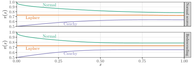
Figure 6: $\pi(x)$ from Theorem 2 for additional score functions not included in Figure 3, when $G$ is standard normal, Laplace (double exponential) or Cauchy, and $\tau=1/2$.

Figure 6 plots $\pi(x)$ as defined in Theorem 2 for additional score functions not included in Figure 3.

References

- (1)
- Boucheron et al. (2013) Boucheron, S., Lugosi, G. and Massart, P. (2013), Concentration inequalities: a nonasymptotic theory of independence, 1st edn, Oxford University Press, Oxford.
- Centers for Disease Control and Prevention National Center for Health Statistics (NCHS)(2017) (CDC) Centers for Disease Control and Prevention (CDC) National Center for Health Statistics (NCHS) (2017), National health and nutrition examination survey data 2009-2016, Technical report, U.S. Department of Health and Human Services, Centers for Disease Control and Prevention, Hyattsville, MD. https://wwwn.cdc.gov/nchs/nhanes/.
- Chernoff (1952) Chernoff, H. (1952), ‘A Measure of Asymptotic Efficiency for Tests of a Hypothesis Based on the sum of Observations’, The Annals of Mathematical Statistics 23(4), 493–507.
- Cornfield et al. (1923/2009) Cornfield, J., Haenszel, W., Hammond, E. C., Lilienfeld, A. M., Shimkin, M. B. and Wynder, E. L. (1923/2009), ‘Smoking and lung cancer: recent evidence and a discussion of some questions.’, International Journal of Epidemiology 38(5), 1175–1191.
- Cramér (1938) Cramér, H. (1938), ‘Sur un nouveau théorème-limite de la théorie des probabilités’, Actualités Scientifiques 736.
- Durrett (2013) Durrett, R. (2013), Probability: Theory and Examples, 4.1 edn.
- Fogarty and Small (2016) Fogarty, C. B. and Small, D. S. (2016), ‘Sensitivity Analysis for Multiple Comparisons in Matched Observational Studies Through Quadratically Constrained Linear Programming’, Journal of the American Statistical Association 111(516), 1820–1830.
- Gilbert et al. (2003) Gilbert, P. B., Bosch, R. J. and Hudgens, M. G. (2003), ‘Sensitivity Analysis for the Assessment of Causal Vaccine Effects on Viral Load in HIV Vaccine Trials’, Biometrics 59(3), 531–541.
- Greifer (2018) Greifer, N. (2018), cobalt: Covariate Balance Tables and Plots. R package version 3.5.0, https://CRAN.R-project.org/package=cobalt.
- Hansen (2004) Hansen, B. B. (2004), ‘Full matching in an observational study of coaching for the SAT’, Journal of the American Statistical Association 99(467), 609–618.
- Hansen and Klopfer (2006) Hansen, B. B. and Klopfer, S. O. (2006), ‘Optimal full matching and related designs via network flows’, Journal of Computational and Graphical Statistics 15(3), 609–627.
- Heller et al. (2009) Heller, R., Rosenbaum, P. R. and Small, D. S. (2009), ‘Split samples and design sensitivity in observational studies’, 104(487), 1090–1101.
- Hewitt and Stromberg (1965) Hewitt, E. and Stromberg, K. R. (1965), Real and Abstract Analysis, Springer-Verlag.
- Howard et al. (2018a) Howard, S. R., Ramdas, A., McAuliffe, J. and Sekhon, J. (2018a), ‘Exponential line-crossing inequalities’, arXiv:1808.03204 [math] .
- Howard et al. (2018b) Howard, S. R., Ramdas, A., McAuliffe, J. and Sekhon, J. (2018b), ‘Uniform, nonparametric, non-asymptotic confidence sequences’, arXiv:1810.08240 [math, stat] .
- Jennison and Turnbull (2000) Jennison, C. and Turnbull, B. W. (2000), Group sequential methods with applications to clinical trials, Chapman & Hall/CRC, Boca Raton.
- Knapp (2007) Knapp, A. W. (2007), Basic Real Analysis, Springer Science & Business Media.
- Lan and DeMets (1983) Lan, K. K. G. and DeMets, D. L. (1983), ‘Discrete Sequential Boundaries for Clinical Trials’, Biometrika 70(3), 659–663.
- Lehmann and Romano (2005) Lehmann, E. L. and Romano, J. P. (2005), Testing statistical hypotheses, 3rd ed edn, Springer, New York.
- Mahaffey et al. (2004) Mahaffey, K. R., Clickner, R. P. and Bodurow, C. C. (2004), ‘Blood organic mercury and dietary mercury intake: National health and nutrition examination survey, 1999 and 2000.’, Environmental health perspectives 112(5), 562.
- Noether (1973) Noether, G. E. (1973), ‘Some Simple Distribution-Free Confidence Intervals for the Center of a Symmetric Distribution’, Journal of the American Statistical Association 68(343), 716–719.
- O’Brien and Fleming (1979) O’Brien, P. C. and Fleming, T. R. (1979), ‘A Multiple Testing Procedure for Clinical Trials’, Biometrics 35(3), 549–556.
- Pimentel (2016) Pimentel, S. D. (2016), ‘Large, sparse optimal matching with r package rcbalance’, Observational Studies 2, 4–23.
- Pimentel et al. (2015) Pimentel, S. D., Kelz, R. R., Silber, J. H. and Rosenbaum, P. R. (2015), ‘Large, sparse optimal matching with refined covariate balance in an observational study of the health outcomes produced by new surgeons’, Journal of the American Statistical Association 110(510), 515–527.
- Pocock (1977) Pocock, S. J. (1977), ‘Group Sequential Methods in the Design and Analysis of Clinical Trials’, Biometrika 64(2), 191–199.
- Robins et al. (2000) Robins, J. M., Rotnitzky, A. and Scharfstein, D. O. (2000), Sensitivity Analysis for Selection bias and unmeasured Confounding in missing Data and Causal inference models, in M. E. Halloran and D. Berry, eds, ‘Statistical Models in Epidemiology, the Environment, and Clinical Trials’, The IMA Volumes in Mathematics and its Applications, Springer New York, pp. 1–94.
- Rosenbaum (1989) Rosenbaum, P. R. (1989), ‘Optimal matching for observational studies’, Journal of the American Statistical Association 84(408), 1024–1032.
- Rosenbaum (2002) Rosenbaum, P. R. (2002), Observational Studies, Springer Series in Statistics, 2nd edn, Springer, New York, NY.
- Rosenbaum (2004) Rosenbaum, P. R. (2004), ‘Design Sensitivity in Observational Studies’, Biometrika 91(1), 153–164.
- Rosenbaum (2010a) Rosenbaum, P. R. (2010a), Design of Observational Studies, Springer Series in Statistics, Springer, New York, NY.
- Rosenbaum (2010b) Rosenbaum, P. R. (2010b), ‘Design Sensitivity and Efficiency in Observational Studies’, Journal of the American Statistical Association 105(490), 692–702.
- Rosenbaum (2011) Rosenbaum, P. R. (2011), ‘A New u-Statistic with Superior Design Sensitivity in Matched Observational Studies’, Biometrics 67(3), 1017–1027.
- Rosenbaum (2012) Rosenbaum, P. R. (2012), ‘An exact adaptive test with superior design sensitivity in an observational study of treatments for ovarian cancer’, The Annals of Applied Statistics 6(1), 83–105.
- Rosenbaum and Rubin (1985) Rosenbaum, P. R. and Rubin, D. B. (1985), ‘Constructing a control group using multivariate matched sampling methods that incorporate the propensity score’, The American Statistician 39(1), 33–38.
- Rosenbaum and Small (2017) Rosenbaum, P. R. and Small, D. S. (2017), ‘An adaptive Mantel–Haenszel test for sensitivity analysis in observational studies’, Biometrics 73(2), 422–430.
- Sen (1970) Sen, P. K. (1970), ‘On Some Convergence Properties of One-Sample Rank Order Statistics’, The Annals of Mathematical Statistics 41(6), 2140–2143.
- Ville (1939) Ville, J. (1939), Étude Critique de la Notion de Collectif., Gauthier-Villars, Paris.
- Yu and Gastwirth (2005) Yu, B. and Gastwirth, J. L. (2005), ‘Sensitivity analysis for trend tests: application to the risk of radiation exposure’, Biostatistics 6(2), 201–209.
- Zubizarreta et al. (2014) Zubizarreta, J. R., Paredes, R. D., Rosenbaum, P. R. et al. (2014), ‘Matching for balance, pairing for heterogeneity in an observational study of the effectiveness of for-profit and not-for-profit high schools in chile’, The Annals of Applied Statistics 8(1), 204–231.