Light-meson leptonic decay rates in lattice QCD+QED
Abstract
The leading electromagnetic (e.m.) and strong isospin-breaking corrections to the and leptonic decay rates are evaluated for the first time on the lattice. The results are obtained using gauge ensembles produced by the European Twisted Mass Collaboration with dynamical quarks. The relative leading-order e.m. and strong isospin-breaking corrections to the decay rates are 1.53(19)% for decays and 0.24(10)% for decays. Using the experimental values of the and decay rates and updated lattice QCD results for the pion and kaon decay constants in isosymmetric QCD, we find that the Cabibbo-Kobayashi-Maskawa matrix element , reducing by a factor of about the corresponding uncertainty in the Particle Data Group review. Our calculation of allows also an accurate determination of the first-row CKM unitarity relation . Theoretical developments in this paper include a detailed discussion of how QCD can be defined in the full QCD+QED theory and an improved renormalisation procedure in which the bare lattice operators are renormalised non-perturbatively into the (modified) Regularization Independent Momentum subtraction scheme and subsequently matched perturbatively at into the W-regularisation scheme appropriate for these calculations.
pacs:
11.15.Ha, 12.15.Lk, 12.38.Gc, 13.20.-vpacs:
11.15.Ha, 12.15.Lk, 12.38.Gc, 13.20.-vI Introduction
In flavour physics the determination of the elements of the Cabibbo-Kobayashi-Maskawa (CKM) matrix CKM , which contains just 4 parameters, from a wide range of weak processes represents a crucial test of the limits of the Standard Model (SM) of particle physics. Inconsistencies with theoretical expectations would indeed signal the existence of new physics beyond the SM and subsequently a detailed comparison of experimental measurements and theoretical predictions would provide a guide towards uncovering the underlying theory beyond the SM. For this to be possible non-perturbative hadronic effects need to be evaluated as precisely as possible and in this paper we report on progress in improving the precision of lattice computations of leptonic decay rates by including radiative corrections and strong isospin-breaking (IB) effects. A summary of our results has been presented in Ref. Giusti:2017dwk ; here we expand on the details of the calculation and include several improvements, most notably the renormalisation of the four-fermion weak operators in the combined QCD+QED theory (see Sec. IV). We also discuss in some detail how one might define the QCD component of the full (QCD+QED) theory (see Sec. II). Although such a separate definition of QCD is not required in order to obtain results computed in the full theory, it is necessary if one wishes to talk about radiative (and strong IB) “corrections” to results obtained in QCD. For this we need to specify what we mean by QCD.
The extraction of the CKM elements from experimental data requires an accurate knowledge of a number of hadronic quantities and the main goal of large-scale QCD simulations on the lattice is the ab initio evaluation of the nonperturbative QCD effects in physical processes. For several quantities relevant for flavour physics phenomenology, lattice QCD has recently reached the impressive level of precision of or even better . Important examples are the ratio of kaon and pion leptonic decay constants and the vector form factor FLAG , which play the central role in the accurate determination of the CKM entries and , respectively. Such lattice computations are typically performed in the isospin symmetric limit of QCD, in which the up and down quarks are mass degenerate () and electromagnetic (e.m.) effects are neglected ().
Isospin breaking effects arise because of radiative corrections and because ; the latter contributions are usually referred to as strong isospin breaking effects. Since both and are of , IB effects need to be included in lattice simulations to make further progress in flavour physics phenomenology, beyond the currently impressive precision obtained in isosymmetric QCD.
Since the electric charges of the up and down quarks are different, the presence of electromagnetism itself induces a difference in their masses, in addition to any explicit difference in the bare masses input into the action being simulated. The separation of IB effects into strong and e.m. components therefore requires a convention. We discuss this in detail in Sec. II, where we propose and advocate the use of hadronic schemes, based on taking a set of hadronic quantities, such as particle masses, which are computed with excellent precision in lattice simulations, to define QCD in the presence of electromagnetism.
In recent years precise lattice results including e.m. and strong IB effects have been obtained for the hadron spectrum; in particular for the mass splittings between charged and neutral pseudoscalar (P) mesons and baryons (see for example, Refs. deDivitiis:2013xla ; Borsanyi:2014jba ). The QED effects were included in lattice QCD simulations using the following two methods:
-
•
QED is added directly to the action and QED+QCD simulations are performed at a few values of the electric charge and the results extrapolated to the physical value of (see, e.g., Refs. Borsanyi:2014jba ; Boyle:2017gzv ; Hansen:2018zre );
-
•
the lattice path-integral is expanded in powers of the two small parameters and . This is the RM123 approach of Refs. deDivitiis:2011eh ; deDivitiis:2013xla ; Giusti:2017dmp which we follow in this paper.
In practice, for all the relevant phenomenological applications it is currently sufficient to work at first order in the small parameters and . The attractive feature of the RM123 method is that it allows one naturally to work at first order in isospin breaking, computing the coefficients of the two small parameters directly. Moreover, these coefficients can be determined from simulations of isosymmetric QCD.
The calculation of e.m. and strong IB effects in the hadron spectrum has a very significant simplification in that there are no infrared (IR) divergences. The same is not true when computing hadronic amplitudes, where e.m. IR divergences are present and only cancel in well-defined, measurable physical quantities by summing diagrams containing real and virtual photons BN37 . This is the case, for instance, for the leptonic and and semileptonic decay rates. The presence of IR divergences requires a new strategy beyond those developed for the calculation of IB effects in the hadron spectrum. Such a new strategy was proposed in Ref. Carrasco:2015xwa , where the determination of the inclusive decay rate of a charged P meson into either a final pair or a final state was addressed.
The e.m. corrections due to the exchange of a virtual photon and to the emission of a real one can be computed non-perturbatively, by numerical simulations, on a finite lattice with the corresponding uncertainties. The exchange of a virtual photon depends on the structure of the decaying meson, since all momentum modes are included, and the corresponding amplitude must therefore be computed non-perturbatively. On the other hand, the non-perturbative evaluation of the emission of a real photon is not strictly necessary Carrasco:2015xwa . Indeed, it is possible to compute the real emission amplitudes in perturbation theory by limiting the maximum energy of the emitted photon in the meson rest-frame, , to a value small enough so that the internal structure of the decaying meson is not resolved. The IR divergences in the non-perturbative calculation of the corrections due to the exchange of a virtual photon are cancelled by the corrections due to the real photon emission even when the latter is computed perturbatively, because of the universality of the IR behaviour of the theory (i.e., the IR divergences do not depend on the structure of the decaying hadron). Such a strategy, which requires an experimental cut on the energy of the real photon, makes the extraction of the relevant CKM element(s) cleaner.
In the intermediate steps of the calculation it is necessary to introduce an IR regulator. In order to work with quantities that are finite when the IR regulator is removed, the inclusive rate is written as Carrasco:2015xwa
| (1) | |||||
where the subscripts indicate the number of photons in the final state, while the superscript pt denotes the point-like approximation of the decaying meson and is an IR regulator. In the first term on the r.h.s. of Eq. (1) the quantities and are evaluated on the lattice. Both have the same IR divergences which therefore cancel in the difference. We use the lattice size as the intermediate IR regulator by working in the QEDL Hayakawa:2008an formulation of QED on a finite volume (for a recent review on QED simulations in a finite box see Ref. Patella:2017fgk ). The difference is independent of the regulator as this is removed Lubicz:2016xro . As already pointed out, since all momentum modes contribute to it, depends on the structure of the decaying meson and must be computed non-perturbatively. The numerical determination of for several lattice spacings, physical volumes and quark masses is indeed the focus of the present study.
In the second term on the r.h.s. of Eq. (1) P is a point-like meson and both and can be calculated directly in infinite volume in perturbation theory, using a photon mass as the IR regulator. Each term is IR divergent, but the sum is convergent BN37 and independent of the IR regulator. In Refs. Carrasco:2015xwa and Lubicz:2016xro the explicit perturbative calculations of and have been performed with a small photon mass or by using the finite volume respectively, as the IR cutoffs.
In Ref. Giusti:2017dwk we have calculated the e.m. and IB corrections to the ratio of and decay rates of charged pions and kaons into muons Giusti:2017dwk , using gauge ensembles generated by the European Twisted Mass Collaboration (ETMC) with dynamical quarks Baron:2010bv ; Baron:2011sf in the quenched QED (qQED) approximation in which the charges of the sea quarks are set to 0. The ratio is less sensitive to various sources of uncertainty than the IB corrections to and decay rates separately. In this paper, in addition to providing more details of the calculation than was possible in Ref. Giusti:2017dwk , we do evaluate the e.m. and strong IB corrections to the decay processes and separately. Since the corresponding experimental rates are fully inclusive in the real photon energy, structure-dependent (SD) contributions to the real photon emission should be included, however according to the Chiral Perturbation Theory (ChPT) predictions of Ref. Cirigliano:2007ga these SD contributions are negligible for both kaon and pion decays into muons. The same is not true to the same extent for decays into final-state electrons (see Ref. Carrasco:2015xwa ) and so in this paper we focus on decays into muons. The SD contributions to are being investigated in an ongoing dedicated lattice study of light and heavy P-meson leptonic decays.
An important improvement presented in this paper is in the renormalisation of the effective weak Hamiltonian. To exploit the matching of the effective theory to the Standard Model performed in Ref. Sirlin:1981ie it is particularly convenient to renormalise the weak Hamiltonian in the W-regularisation scheme. The renormalisation is performed in two steps. First of all, the lattice operators are renormalised non-perturbatively in the (modified) Regularization Independent Momentum subtraction (RI′-MOM) scheme at and to all orders in the strong coupling . Because of the breaking of chiral symmetry in the twisted mass formulation we have adopted in our study, this renormalisation includes the mixing with other four-fermion operators of different chirality. In the second step we perform the matching from the RI′-MOM scheme to the W-regularisation scheme perturbatively. By calculating and including the two-loop anomalous dimension at , the residual truncation error of this matching is of , reduced from in our earlier work Carrasco:2015xwa .
The main results of the calculation are presented in Sec. VI together with a detailed discussion of their implications. Here, we anticipate some key results: After extrapolation of the data to the physical pion mass, and to the continuum and infinite-volume limits, the isospin-breaking corrections to the leptonic decay rates can be written in the form:
| (2) | |||||
| (3) |
where is the leptonic decay rate at tree level in the Gasser-Rusetsky-Scimemi (GRS) scheme which is a particular definition of QCD Gasser:2003hk (see Sec. II.2.2 below). The corrections are about 1.5% for the pion decays and 0.2% for the kaon decay, in line with naïve expectations. Taking the experimental value of the rate for the decay, Eq. (3) together with obtained using the lattice determination of the kaon decay constant we obtain , in agreement with the latest estimate , recently updated by the Particle Data Group (PDG) PDG but with better precision. Alternatively, by taking the ratio of and decay rates and the updated value from super-allowed nuclear beta decays Hardy:2016vhg , we obtain . The unitarity of the first row of the CKM matrix is satisfied at the per-mille level; e.g. taking the value of from the ratio of decay rates and PDG , we obtain . See Sec. VI for a more detailed discussion of our results and their implications.
The plan for the remainder of this paper is as follows. A discussion of the relation between the “full” QCD+QED theory, including e.m. and strong IB effects, and isosymmetric QCD without electromagnetism is given in Sec. II. We discuss possible definitions of QCD in the full QCD+QED theory, and in particular we define and advocate hadronic schemes as well as the GRS scheme which is conventionally used Gasser:2003hk . In Sec. III we present the calculation of the relevant amplitudes using the RM123 approach. The renormalisation of the bare lattice operators necessary to obtain the effective weak Hamiltonian in the -regularization scheme is performed in Sec. IV, while the subtraction of the universal IR-divergent finite volume effects (FVEs) is described in Sec. V. The lattice data for the e.m. and strong IB corrections to the leptonic decay rates of pions and kaons are extrapolated to the physical pion mass, to the continuum and infinite volume limits in Sec. VI. Finally, Sec. VII contains our conclusions. There are four appendices. The lattice framework and details of the simulation are presented in Appendix A. Appendix B contains a detailed discussion of the relation between observables in the full theory and in QCD, expanding on the material in Sec. II. An expanded discussion of the renormalisation of the effective weak Hamiltonian, including electromagnetic corrections, is presented in Appendices C, which contains a general discussion of the non-perturbative renormalisation in the RI'-MOM scheme and D in which issues specific to the twisted mass formulation are discussed.
II Defining QCD in the full theory (QCD+QED)
Before presenting the detailed description of our calculation of leptonic decay rates, we believe that it is useful to discuss the relation between the “full ” QCD+QED theory, that includes explicit e.m. and strong isospin breaking effects, and QCD without electromagnetism (denoted in the following as the full theory and QCD, respectively).
The action of the full theory can be schematically written as
| (4) |
Here is the strong coupling constant, is a discretisation of the gluon action, is the preferred discretisation of the Maxwell action of the photon, is the kinetic term for the quark with flavour , including the interaction with the gluon and photon fields, is the mass term, and are respectively the kinetic and mass terms for the lepton (for details see Appendix B). For fermion actions which break chiral symmetry, such as the Wilson action, a counterterm is needed to remove the critical mass and has to be replaced with . A mass counterterm is in principle needed also in the case of the lepton, but at leading order in the lepton critical mass can be ignored.
At the level of precision to which we are currently working it is only the full theory, as defined in Eq. (4), which is expected to reproduce physical results and that is therefore unambiguous. Nevertheless, a frequently asked question is what is the difference between the results for a physical quantity computed in the full theory and in pure QCD, and how big are the strong isospin-breaking effects compared to the e.m. corrections. We particularly wish to underline that in order to properly formulate such questions it is necessary to carefully define what is meant by QCD. It is naturally to be expected that in QCD alone physical quantities will not be reproduced with a precision of better than and this of course is the motivation for including QED. In order to define what is meant by QCD at this level of precision it is necessary to state the conditions which are used to determine the quark masses and the lattice spacing. The separation of the full theory into QCD and the rest is therefore prescription dependent.
In Ref. deDivitiis:2013xla the subtle issue of a precise definition of QCD has been discussed by using the scheme originally proposed in Ref. Gasser:2003hk , which we refer to as the GRS scheme and which has been widely used deDivitiis:2013xla ; Giusti:2017dmp ; Giusti:2017dwk . In the following and in Appendix B we present an extended and detailed discussion by introducing the hadronic schemes. Indeed, in light of the fact that hadron masses can nowadays be computed very precisely, we strongly suggest using hadronic schemes in future lattice calculations of QED radiative corrections. At the end of this section we discuss the connection with the GRS scheme that we had adopted at the time in which this calculation was started and that, for this reason, has been used in this work. A summary of the ideas discussed here has already been presented in Ref. Giusti:2018guw .
II.1 Renormalisation of the full theory
The main difference in the steps required to renormalise the full theory compared to the procedure in QCD is the presence of a massless photon and the corresponding finite-volume (FV) corrections which appear as inverse powers of , where is the spatial extent of the lattice and the volume . By contrast, in QCD for leptonic and semileptonic decays the FV corrections are exponentially small in the volume. In the discussion below, if necessary, we imagine that the chiral Ward identities have been imposed to determine the critical masses Bochicchio:1985xa .
A possible strategy in principle is the following:
-
1.
Fix the number of lattice points , e.g. and , where and are the temporal and spatial extents of the lattice and the lattice spacing will be determined later. (The specific choice is convenient for illustration but not necessary for the following argument.)
-
2.
Using a four-flavour theory for illustration, we now need to determine the four physical bare quark masses, the bare electric charge and the lattice spacing. To this end we need to compute six quantities, e.g. the five dimensionless ratios111An alternative procedure to determine the bare electric charge would be the evaluation of the hadronic corrections to a leptonic observable.
(5) as well as a dimensionful quantity, e.g. the mass of the baryon, computed in lattice units, from which the lattice spacing can be determined after extrapolation to the infinite volume limit (see below):
(6) where GeV is the physical value of the mass of the baryon. For illustration we are considering the masses of QCDQED stable pseudoscalar mesons in the numerators of the dimensionless ratios (5) and using to determine the lattice spacing, but of course other quantities can be used instead. For example, in the four flavour theory that we are considering here one can in principle avoid potentially very noisy baryon observables by using one of the charmed mesons masses already considered above to set the scale. The choice of setting the scale with a charmed-meson observable could however, generate significant cutoff effects and reduce the sensitivity to the charm mass. In Eqs. (5) - (6) we have used instead of to highlight that the infinite-volume limit should be taken at fixed lattice spacing (see Eq. (7) below). The quantity m represents the vector of bare quark masses . Note that in the RM123 strategy, since one works at first order in , it is not necessary to impose a renormalisation condition to fix the e.m. coupling deDivitiis:2013xla ; Giusti:2017dmp . In this case the electric charge can simply be fixed to the Thomson limit, i.e. , and becomes a predictable quantity. For the remainder of this section, we assume that we are working to and only consider the four ratios (i=1,2,3,4) as well as when discussing the calibration of the lattices. Notice also that at first order in the cannot decay in two photons, so that it can also be used in the calibration procedure (see section III below).
-
3.
Up to this point the procedure is the standard one used in QCD simulations. The difference here is in the FV effects which behave as inverse powers of . We therefore envisage extrapolating the ratios to the infinite-volume limit:
(7) -
4.
For a given discretisation and choice of , the physical bare quark masses, , and the electric charge, , are defined by requiring that the five ratios take their physical values
(8) In practice, of course, depending on the specific choice of the ratios , this will require some extrapolations of results obtained at different values of the bare quark masses and electric charge.
-
5.
The lattice spacing at this value of can now be defined to be
(9) Note that with such a procedure the bare parameters and the lattice spacing do not depend on the lattice volume.
-
6.
At first order in isospin breaking, i.e. , the renormalisation of the lepton masses is performed perturbatively, by requiring that the on-shell masses correspond to the physical ones. If one wishes to go beyond first order, when hadronic effects first enter, then the physical lepton masses should be added to the quantities used in the non-perturbative calibration. The bare lepton masses, together with the other parameters, should be chosen such that, in addition to satisfying the conditions in Eq. (5), the lepton-lepton correlators decay in time as , where is the physical mass of the lepton .
In Eq. (7) we have taken the infinite-volume limit of the computed hadron masses. By working in the QED finite-volume formulation of QED, if for each hadron the FV corrections of order can be neglected, then the extrapolation to the infinite-volume limit can be avoided by making use of the formula Hayakawa:2008an ; Borsanyi:2014jba (similar formulae also exist for other finite-volume formulations of the theory Lucini:2015hfa )
| (10) |
where is the charge of the hadron and is a known universal constant (independent of the structure of the hadron ). Equation (10) can be used to determine the infinite-volume mass of the hadron from the value measured on the finite-volume , up to corrections of order of . (In any case, even if one wishes to study the behaviour with by performing simulations at different volumes, the subtraction of the universal and terms using Eq. (10) is a useful starting point; the residual leading behaviour of hadronic masses is then of .)
II.2 Defining observables in QCD
The procedure discussed in section II.1 provides a full framework with which to perform lattice simulations of QCD together with isospin-breaking effects including radiative corrections. Nevertheless, one may wish to ask how different are the results for some physical quantities in the full theory (QCD+QED) and in QCD alone. We stress again that, under the assumption that isospin breaking effects are not negligible, QCD by itself is an unphysical theory and requires a definition. Different prescriptions are possible and, of course, lead to different results in QCD. In this section we propose and advocate hadronic schemes, based on the nonperturbative evaluation of a set of hadronic masses in lattice simulations and contrast this with schemes based on equating the renormalised strong coupling and masses in some renormalisation scheme and at a particular renormalisation scale which have been used previously.
We recall that the QCD action is given by
| (11) |
where the kinetic term only includes the gluon links and the subscripts 0 indicate that the bare coupling and masses are different from those in the full theory of Eq. (4). Indeed the two theories have different dynamics that, in turn, generate a different pattern of ultraviolet divergences. The difference in the bare parameters of the two theories, for all schemes used to define QCD, can in fact be ascribed to the necessity of reabsorbing the different ultraviolet singularities. In what follows we present two different approaches to making the choice of the parameters and . Explicit details of the lattice action, discretised using the Wilson formulation for the fermions for illustration, are presented in Appendix B.1.
II.2.1 Defining observables in QCD: hadronic schemes
In hadronic schemes we choose a value of and determine the bare quark masses and the lattice spacing imposing the same conditions as for the full theory for the ratios evaluated at vanishing electric charge, i.e. following steps 1 - 5 in Sec. II.1 without imposing any constraint on the ratio . We repeat that, for illustration we define the bare quark masses and lattice spacing using the five ratios , but other hadronic quantities could be used instead, both in the full theory and in QCD. These parameters differ by terms of order from those in the full theory. For this discussion, we make the natural and convenient choice . (In order to make the perturbative expansion in Eq. (125) the difference should be less than .) With this choice, the lattice spacings in QCD () and in the full theory () are therefore given by
| (12) |
To illustrate the procedure imagine that we wish to calculate an observable of mass dimension 1, for example the mass of a hadron which has not been used for the calibration. The generalisation to other cases is straightforward and presented in Appendix B. At a fixed value of , we denote the best estimate of the observable , which is the one obtained in the full theory, by , and that obtained in QCD as defined above by :
| (13) |
We define the difference of the two as being due to QED effects, . There are 3 contributions to :
- 1.
-
2.
The second contribution comes from the fact that the bare quark masses appearing in Eq. (4) and Eq. (11) are different. The corresponding quark-mass counterterms must therefore be inserted into the correlation functions used to determine . We stress that the need to include quark-mass counterterms is generic and arises from the requirement that the conditions being used to determine the quark masses must be satisfied both in the full theory and in QCD (for the hadronic scheme being used for illustration we impose that the conditions in Eq. (8) are satisfied in both theories).
-
3.
Finally we must account for the difference in the lattice spacings in the full theory and QCD.
Combining these contributions we arrive at
| (14) |
where we have combined the contributions to the correlation functions from the exchange of virtual photons and from the insertion of the mass counterterms into .
The detailed derivation of Eq. (14) is presented in Appendix B but some further comments may be helpful here. The first term on the right-hand side is one that can be calculated within QCD alone. It has a well defined continuum limit as does the sum of all the terms in Eq. (14). This term allows us to define what is the difference between QCD (defined as above) and the full theory in the hadronic scheme: .
An important feature of the RM123 approach which we follow in the numerical study presented below, is that the terms are computed explicitly and so we do not have to take the difference between numerical calculations performed in the full theory and in QCD. Each of the terms on the right-hand side of Eq. (14) is calculated directly. We now explain the procedure in some more detail by assuming that terms of order are negligible (the extension to higher orders in is straightforward).
-
1.
Correlation functions corresponding to diagrams with the exchange of a virtual photon and to the insertion of the mass counterterms are already of and are calculated directly in QCD. The term proportional to the time separation in the correlation functions gives us the mass shift () and for the five masses (or mass differences) in the ratios () in Eq. (5);
-
2.
In the hadronic scheme being used for illustration, we impose the condition that the four ratios are the same in QCD and in the full theory. This corresponds to requiring that
(15) The QED contribution to the left-hand side is different from zero (and also ultraviolet divergent) and we require the terms proportional to the counterterms to cancel this contribution. We therefore (in principle) scan the values of the four mass counterterms () until the four conditions (15) are satisfied. Also in this case no subtraction of results obtained in the full theory and in QCD is necessary.
- 3.
We have devoted a considerable discussion to the definition of the isospin-breaking effects due to electromagnetism, . Having done this, the subsequent definition of the strong isospin breaking effects is straightforward. To do this however, we need to define the isosymmetric theory (labelled by “ISO”) by imposing appropriate conditions to determine the bare quark masses and the lattice spacing. Since , in the theory we need to determine only three quark masses and hence we only need three conditions, e.g. we can use the ratios in Eq. (5) to determine the physical bare quark masses. For the determination of the lattice spacing we have two options. The simplest one is to work in a mass–independent scheme and set the lattice spacing in the isosymmetric theory, , equal to the one of QCD with , i.e. . Notice that this choice is fully consistent with renormalisation because the ultraviolet divergences of the theories that we are considering do not depend on the quark masses. Note however, that they do depend instead on the electric charge. The other option is that we set the lattice spacing in the isosymmetric theory by using in Eq. (9). The difference between the two options is due to cutoff effects that disappear once the continuum limit is taken consistently. The strong isospin breaking correction to the observable can now be defined by
| (16) |
where is the value of the observable obtained in isosymmetric QCD. With these definitions we have the natural relation . We underline however that depends on the quantities used for calibration, both in 4-flavour QCD and in isosymmetric QCD.
II.2.2 Defining QCD: the GRS scheme
A different prescription, called the GRS scheme, was proposed in Ref. Gasser:2003hk to relate the bare quark masses and bare coupling of QCD ( and ) to those in the full theory ( and ). This prescription has been adopted in Refs. deDivitiis:2013xla ; Giusti:2017dmp ; Giusti:2017dwk . In the GRS approach, instead of determining the bare parameters of QCD by requiring that the chosen hadronic masses in QCD are equal to their physical values, one imposes that the renormalised parameters in a given short–distance scheme (e.g. the scheme) and at a given scale are equal in the full and QCD theories.
A consistent procedure is the following:
-
1.
The full theory is renormalised by using a physical hadronic scheme as discussed in subsection II.1. This means that for each chosen value of we know the corresponding physical value of the bare electric charge and of the lattice spacing .
-
2.
The renormalisation constants (RCs) of the strong coupling constant and of the quark masses are computed in a short–distance mass–independent scheme both in the full theory and in the theory at vanishing electric charge.
-
3.
In order to set the bare parameters of QCD at a given value of the lattice spacing we now chose a matching scale and impose that the renormalised strong coupling constant and the renormalised quark masses are the same as in the full theory. In practice we might want to simulate QCD at the same values of the lattice spacing used in the full theory simulations. In this case the matching conditions are
(17) where indicates quantities in the QCD+QED theory. Notice that quarks with the same electric charge have the same RC, e.g. , and that the quark mass RC at vanishing electric charge is flavour independent, .
-
4.
In order to define isosymmetric QCD by using this approach, the bare up–down quark mass is determined from
(18)
Some remarks are in order at this point. The GRS scheme is a short–distance matching procedure that can also be used to match the theories at unphysical values of the renormalised electric charge and/or quark masses with the physical theory.
By following the procedure outlined above one can perform lattice simulations of the full theory and of (isosymmetric) QCD at the same value of the lattice spacing but, consequently, at different values of the bare strong coupling constant. This is different from the strategy outlined in the previous subsection where, by using hadronic schemes, it was more natural to chose the same value of the bare strong coupling at the price of having two different lattice spacings. The absence of the lattice spacing counterterm (see Eq. (14) above) in the GRS scheme is compensated from the presence of the counterterm originating from the difference of the bare strong coupling constants in the two theories.
A remark of some practical relevance concerns the possibility of implementing hadronically the GRS scheme. To this end, note that in the GRS scheme the dimensionless ratios will not be equal to the corresponding physical values and the difference can be parametrized as follows
| (19) |
where the are order and depend on the chosen matching scheme and also on the chosen matching scale. Once the (and hence the ) are known, for example from a particularly accurate lattice simulation, then they can be used in other lattice computations. The bare quark masses are then determined by requiring that the in (isosymmetric) QCD reproduce as given by Eq.(19), and, at this stage, the GRS scheme can be considered to be a hadronic one as it is defined in terms of non-perturbatively computed quantities (in this case meson masses). We stress however that this requires prior knowledge of the .
Of course other schemes are also possible. In general, the provide a unifying language to discuss the different schemes for the definition of (isosymmetric) QCD in the presence of electromagnetism; in physical hadronic schemes the while in the GRS and other schemes they are of order . For later use, we make the simple observation that two schemes can be considered to be equivalent in practice if the in the two schemes are equal within the precision of the computations.
Although the GRS scheme is perfectly legitimate, we advocate the use of physical hadronic schemes in future lattice calculations. For lattice simulations of physical quantities, a non-perturbative calibration of the lattice is necessary in general, but the renormalisation required for the GRS conditions in Eq. (17) is not generally necessary (except perhaps for the determination of the renormalised coupling and quark masses themselves). Now that hadronic masses are calculated with excellent precision in lattice simulations and their values are well known from experimental measurements, it is natural to use hadronic schemes. By contrast, the renormalised couplings and masses are derived quantities which are not measured directly in experiments. In spite of this, as explained above, at the time that our computation was started we chose to use the GRS scheme. Of course the physical results in the full theory do not depend on this choice.
III Evaluation of the amplitudes
At first order in and the inclusive decay rate (1) can be written as
| (20) |
where is the tree-level decay rate given by
| (21) |
and and are the mass and decay constant of the charged P-meson mass defined in isosymmetric QCD in the chosen scheme.
The decay constant is defined in terms of the matrix element of the QCD axial current (in the continuum) as
| (22) |
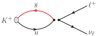
where the initial state meson is at rest. The decay rate is obtained from the insertion of the lowest-order effective Hamiltonian
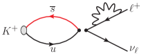
| (23) |
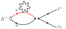
as depicted in the Feynman diagram of Fig. 1, where the decay of a charged kaon is shown as an example. At lowest order in the two full dots in the figure represent the two currents in the bare four-fermion operator
| (24) |
whereas at order they will denote the insertion of the renormalised operator in the W-regularisation as defined in Sec. IV.
In order to compare our results for the e.m. and strong IB corrections to those obtained in Ref. Cirigliano:2011tm and adopted by the PDG PDG ; Rosner:2015wva however, we will use a modified expression:
| (25) |
where is given by
| (26) |
and is the physical mass of the charged P-meson including both e.m. and leading-order strong IB corrections.
The quantity encodes both the e.m. and the strong IB leading-order corrections to the tree-level decay rate. Its value depends on the prescription used for the separation between the QED and QCD corrections, while the quantity
| (27) |
is prescription independent Gasser:2010wz to all orders in both and .
The quantity may be used to set the lattice scale instead of the baryon mass. The physical value can be obtained by taking the experimental pion decay rate s-1 from the PDG PDG and the result for determined accurately from super-allowed -decays in Ref. Hardy:2016vhg . Consequently, one may replace with (as the denominator of the ratios in Eqs. (5)), with in the ratio (when working at leading order in ) and set the electron charge directly to its Thomson’s limit (instead of using the ratio ), namely
| (28) |
Note that for the present study we were unable to use to determine the lattice spacing because the corresponding baryon correlators were unavailable. The choice of using instead to set the scale clearly prevents us from being able to predict the value of . This is one of the reasons why we advocate the use of hadronic schemes with hadron masses as experimental inputs for future lattice calculations. However, as already explained above, in this work we renormalise the QCD theory using the same set of hadronic inputs adopted in our quark-mass analysis in Ref. Carrasco:2014cwa , since we started the present calculations using the RM123 method on previously generated isosymmetric QCD gauge configurations from ETMC (see Appendix A). The bare parameters of these QCD gauge ensembles were fixed in Ref. Carrasco:2014cwa by using the hadronic scheme corresponding to MeV, MeV and MeV, while was chosen to be equal to the experimental -meson mass, MeV PDG . Note that in the absence of QED radiative corrections reduces to the conventional definition of the pion decay constant . The superscript FLAG has been used because the chosen values of three out of the four hadronic inputs had been suggested in the previous editions of the FLAG review FLAG . For this reason we refer to the scheme defined from these inputs as the FLAG scheme.
We have calculated the same input parameters (28) used in the FLAG scheme also in the GRS scheme (corresponding to the scheme at GeV) obtaining222These values differ slightly from those obtained in Ref. Giusti:2017dmp , since we have now included the non-factorisable corrections of order (with ) to the mass renormalisation constant (see the coefficient in Eq. (40) and in Table 1 below). We take the opportunity to update Eqs. (8), (10), (14) and (15) of Ref. Giusti:2017dmp with , , MeV and MeV.: MeV, MeV, MeV and MeV (see Eq. (111) in Sec. VI below). Therefore, the values of the inputs determined in the GRS scheme differ at most by from the corresponding values adopted in Ref. Carrasco:2014cwa for the isosymmetric QCD theory and the differences are at the level of our statistical precision. Thus, the result of our analysis of the scheme dependence can be summarized by the conclusion that the FLAG and GRS schemes can be considered to be equivalent at the current level of precision. Nevertheless, we have used the results of this analysis to estimate the systematic error on our final determinations of the isospin breaking corrections induced by residual scheme uncertainties (see the discussion at the end of Sec. VI).
In light of this quantitative analysis, given the numerical equivalence of the two schemes at the current level of precision, in the rest of the paper we shall compare our results obtained in the GRS scheme with the results obtained by other groups using the FLAG scheme and we shall not use superscripts to distinguish between the two schemes.
The correction , defined in Eq. (25), is given by (see Ref. Carrasco:2015xwa )
| (29) |
where
-
i)
the term containing comes from the short-distance matching between the full theory (the Standard Model) and the effective theory in the -regularisation Sirlin:1981ie ;
-
ii)
the quantity represents the correction to the tree-level decay rate for a point-like meson (see Eq. (1)), which can be read off from Eq. (51) of Ref. Carrasco:2015xwa . The cut-off on the final-state photon’s energy, , must be sufficiently small for the point like-approximation to be valid;
-
iii)
is the e.m. and strong IB correction to the decay amplitude with the corresponding correction to the amplitude with a point-like meson subtracted (this subtraction term is added back in the term , see Eq. (1)).
-
iv)
are the e.m. and strong IB corrections to the mass of the P-meson. The correction proportional to is present because of the definition of in terms of the amplitude and of the meson mass in Eq. (22).
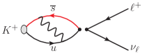
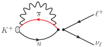
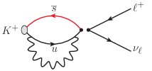
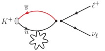
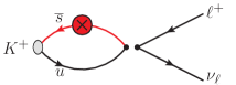
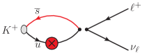
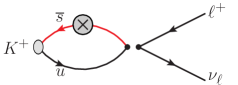
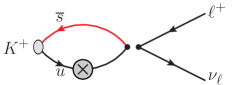
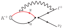
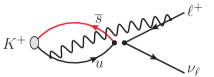
Since we adopt the qQED approximation, which neglects the effects of the sea-quark electric charges, the calculation of and only requires the evaluation of the connected diagrams. These are shown in Figs. 1 - 5 for the case of decays. At the diagram in Fig. 1 corresponds to the insertion of the operator renormalised in the W-renormalisation scheme.
In Eq. (29) and contain both the e.m. and the strong IB leading-order corrections
| (30) | |||||
| (31) |
where is the e.m. correction from both the matching of the four-fermion lattice weak operator to the W-renormalisation scheme and from the mixing with several bare lattice four-fermion operators generated by the breaking of chiral symmetry with the twisted-mass fermion action which we are using. Both the matching and the mixing will be discussed and calculated in Sec. IV. As already pointed out, the renormalised operator, defined in the W-renormalisation scheme, is inserted in the diagram of Fig. 1. As for the diagrams of Figs. 2 - 5, which are already of order and , it is sufficient to insert the weak current operator renormalised in QCD only.
In Eqs. (30) and (31) the quantity () represents the strong IB corrections proportional to and to the diagram of Fig. 4(b), while the other terms are QED corrections coming from the insertions of the e.m. current and tadpole operators, of the pseudoscalar and scalar densities (see Refs. deDivitiis:2013xla ; deDivitiis:2011eh ). The term () is generated by the diagrams of Fig. 2(a-c), () by the diagrams of Fig. 2(d-e), () by the diagrams of Fig. 3(a-b) and () by the diagrams of Fig. 4(a-b). The term corresponds to the exchange of a photon between the quarks and the final-state lepton and arises from the diagrams in Fig. 5(a-b). The term corresponds to the contribution to the amplitude from the lepton’s wave function renormalisation; it arises from the self-energy diagram of Fig. 5(c). The contribution of this term cancels out in the difference and could be therefore omitted, as explained in the following section. The different insertions of the scalar density encode the strong IB effects together with the counter terms necessary to fix the masses of the quarks. The insertion of the pseudoscalar density is peculiar to twisted mass quarks and would be absent in standard Wilson (improved) formulations of QCD.
In the following subsection we discuss the calculation of all the diagrams that do not involve the photon attached to the charged lepton line. The determination of the contributions and will be described later in subsection III.2.
III.1 Quark-quark photon exchange diagrams and scalar and pseudoscalar insertions
The terms and () can be extracted from the following correlators:
| (32) | |||||
| (33) | |||||
| (34) | |||||
| (35) |
where is the photon propagator, is the local version of the hadronic weak current renormalised in QCD only333In our maximally twisted-mass setup, in which the Wilson -parameters and are always chosen to be opposite (see Appendix A), the vector (axial) weak current in the physical basis renormalises multiplicatively with the RC () of the axial (vector) current for Wilson-like fermions, i.e. and (see Appendix D).
| (36) |
is the (lattice) conserved e.m. current444The use of the conserved e.m. current guarantees the absence of additional contact terms in the product .
| (37) | |||||
and is the tadpole operator
| (38) | |||||
In Eqs. (32) - (35) is the interpolating field for a P-meson composed by two valence quarks and with charges and . The Wilson -parameters and are always chosen to be opposite (see Appendix A). We have also chosen to place the weak current at the origin and to create the P-meson at a negative time , where and are sufficiently large to suppress the contributions from heavier states and from the backward propagating P-meson (this latter condition may be convenient but is not necessary). In Eq. (35) is the mass RC in pure QCD, which for our maximally twisted-mass setup is given by , where is the RC of the pseudoscalar density determined in Ref. Carrasco:2014cwa . The quantity is related to the e.m. correction to the mass RC
| (39) |
and can be written in the form
| (40) |
where is the pure QED contribution at leading order in , given in the scheme at a renormalisation scale by Martinelli:1982mw ; Aoki:1998ar
| (41) |
where is the fractional charge of the quark and takes into account all the corrections of order with .
The quantity is computed non-perturbatively in section IV and represents the QCD corrections to the “naive factorisation” approximation (i.e. ) introduced in Refs. Giusti:2017dmp ; Giusti:2017jof .
Analogously, the term and can be extracted from the correlator
| (42) |
where, following the notation of Ref. Giusti:2017dmp , we indicate with and the renomalized masses of the quark with flavour in the full theory and in isosymmetric QCD only, respectively. We stress again that the separation between QCD and QED corrections is prescription dependent and in this work we adopt the GRS prescription of Refs. deDivitiis:2013xla ; Giusti:2017dmp ; Giusti:2017dwk , where
| (43) |
Thus, in Eq. (42), the only relevant quark mass difference is , whose value in the scheme was found to be equal to MeV Giusti:2017dmp using as inputs the experimental values of the charged and neutral kaon masses.
Following Ref. deDivitiis:2013xla we form the ratio of with the corresponding tree-level correlator
| (44) |
and at large time distances we obtain ()
| (45) | |||||
where
| (46) |
is the coupling of the interpolating field of the P-meson with its ground-state in isosymmetric QCD. The term proportional to in the r.h.s. of Eq. (45) is related to the e.m. and strong IB corrections of the meson mass.
The function in the square brackets on the r.h.s. of Eq. (45) is an almost linear function of . Thus, the correction to the P-meson mass, , can be extracted from the slope of the ratio and the quantity from its intercept. As explained in Ref. Carrasco:2015xwa , in order to obtain the quantity the correction is separately determined by evaluating a correlator similar to those of Eqs. (32) - (35), in which the weak operator is replaced by the P-meson interpolating field .
For illustration, in Fig. 6 we show the ratios for the charged kaon () obtained from the ensemble D20.48 (see Appendix A). The top panel contains the ratio , the ratio is shown in the middle panel and the ratios and are presented in the bottom panel.
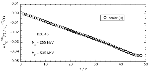
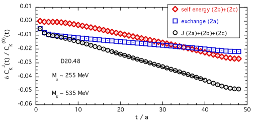
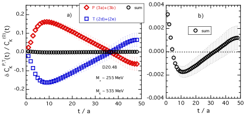
We find: i) the contributions and are separately large, but strongly correlated, since the tadpole insertion dominates the values of the e.m. shift of the critical mass (see Ref. Giusti:2017dmp ). In the chiral limit they would cancel, but at finite masses the sum is small and linear in . Because of the correlations it can nevertheless, be determined quite precisely (see the bottom right-hand plot of Fig. 6) where the sum is presented on an expanded scale. ii) the time dependence of the ratio is almost linear in the time interval where the ground state is dominant.
III.2 Crossed diagrams and lepton self-energy
The evaluation of the diagrams 5(a) - (b), corresponding to the term in Eq. (30), can be obtained by studying the correlator Carrasco:2015xwa
| (47) | |||||
where stands for the free twisted-mass propagator of the charged lepton. For the numerical analysis we have found it to be convenient to saturate the Dirac indices by inserting on the r.h.s. of Eq. (47) the factor , which represents the lowest order “conjugate” leptonic () amplitude, and to sum over the lepton polarizations. In this way we are able to study the time behaviour of the single function .
The corresponding correlator at lowest order () is
| (48) |
In Eqs. (47) and (48) the contraction between the weak hadronic current [see Eq. (36)] and its leptonic () counterpart gives rise to two terms corresponding to the product of either the temporal or spatial components of these two weak currents, which are odd and even under time reversal, respectively. Thus, on a lattice with finite time extension , for and one has
| (49) |
where , and
| (50) |
is the relevant leptonic trace evaluated on the lattice using for the charged lepton the free twisted-mass propagator and for the neutrino the free Wilson propagator in the P-meson rest frame [].
Similarly, for the lowest-order correlator one has
| (51) |
where is the renormalised axial amplitude evaluated on the lattice in isosymmetric QCD in the P-meson rest frame, namely
| (52) |
The effect of the different signs of the backward-propagating signal in Eq. (49) can be removed by introducing the following new correlators:
| (53) |
where
| (54) |
Thus, the quantity can be extracted from the plateau of the ratio at large time separations, viz.
| (55) |
Note that the diagrams in Fig. 5(a) - (b) do not contribute to the electromagnetic corrections to the masses of the mesons and therefore the ratio (55) has no slope in in contrast to the ratios (45). Moreover, the explicit calculation of on the lattice is not required.
In terms of the lattice momenta and , defined as
| (56) | |||||
| (57) |
the energy-momentum dispersion relations for the charged lepton and the neutrino in the P-meson rest frame are given by
| (58) | |||||
| (59) |
The 3-momentum of the final-state lepton () must be chosen to satisfy the equation
| (60) |
Thus, for any given simulated P-meson mass , the 3-momentum , is calculated from Eq. (60) and is injected on the lattice using non-periodic boundary conditions Bedaque:2004kc ; deDivitiis:2004kq for the lepton field. A simple calculation yields
| (61) |
In Fig. 7 we show the correlators , , and for decays, multiplied by the ground-state exponential. These were obtained on the gauge ensembles A40.24 and D30.48 of Appendix A.
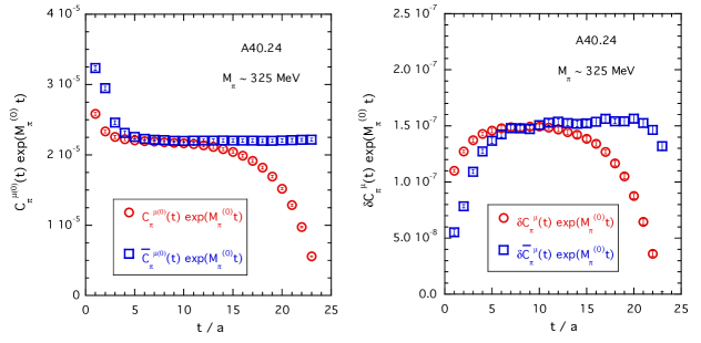
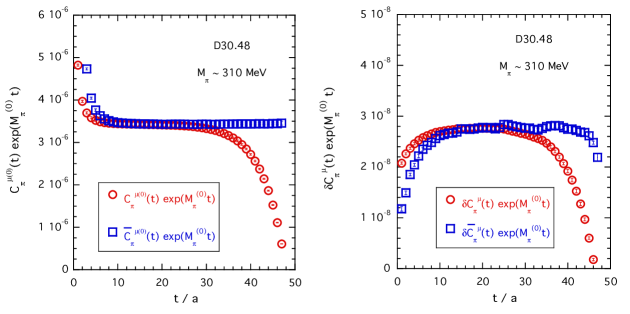
The subtraction of the backward signals, needed for extracting directly the quantity given by Eq. (54), is beneficial also for extending the time region from which (as well as the ratio ) can be determined.
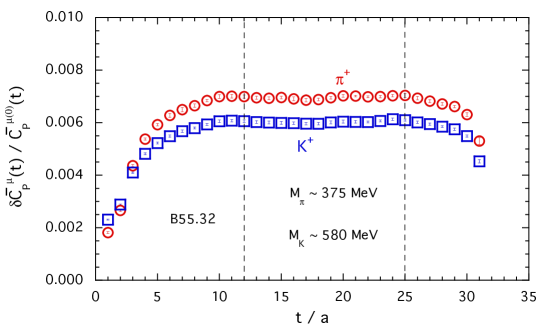
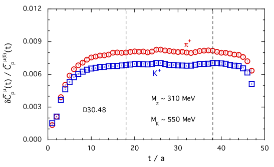
The quality of the signal for the ratio is illustrated in Fig. 8 for charged kaon and pion decays into muons for the case of the ensembles B55.32 and D30.48.
The calculation of the correction due to the diagram 5(c) is straightforward, since it is obtained by simply multiplying the lowest order amplitude, , by the one-loop lepton self-energy evaluated on the lattice.
IV Renormalisation of the effective Hamiltonian and chirality mixing
In this section we provide the basic formalism to derive the e.m. corrections to the RCs non-perturbatively; further details of the calculation will be presented in a forthcoming publication dicarlo . This procedure relates the bare lattice operators to those in the RI'-MOM (and similar) renormalisation schemes up to order and to all orders in . We also improve the precision of the matching of the weak operator (see Eq. (24)) renormalised in the RI'-MOM scheme to that in the W-regularisation by calculating the coefficient of the term proportional to in the matching coefficient. Using the two-loop anomalous dimension thus determined, we can evolve the operator to the renormalisation scale of . Following this calculation the error due to renormalisation is reduced from order to order .
The effective Hamiltonian, including the perturbative electroweak matching with the Standard Model Sirlin:1981ie , can be written in the form
| (62) |
where the term proportional to the logarithm has been already included in Eq. (29) and is the operator renormalised in the W-regularisation scheme, which is used to regularise the photon propagator. Since the W-boson mass is too large to be simulated on the lattice, a matching of the lattice weak operator to the W-regularisation scheme is necessary. In addition, for lattice formulations which break chiral symmetry, like the one used in the present study, the lattice weak operator mixes with other four-fermion operators of different chirality.
IV.1 The renormalised weak operator in the W-regularisation scheme
In order to obtain the operator renormalised in the W-regularisation scheme, we start by renormalising the lattice four-fermion operator defined in Eq. (24) in the RI'-MOM scheme Martinelli:1994ty , obtaining , and then perturbatively match the operator to the one in the W-regularization Carrasco:2015xwa
| (63) |
The coefficient can be computed by first evolving the operator in the RI' scheme to the scale and then matching it to the corresponding operator in the W-scheme. The coefficient can therefore be written as the product of a matching coefficient and an evolution operator
| (64) |
Below we will only consider terms of first order in and, therefore we will consistently neglect the running of .
We note that the original bare lattice operators and are gauge invariant, and thus the corresponding matching coefficients are gauge invariant. This is not the case for that instead depends not only on the external states chosen to define the renormalisation conditions, but also on the gauge. Consequently the matching coefficient and the evolution operator are in general gauge dependent. However, at the order of perturbation theory to which we are working, the evolution operator turns out to be both scheme and gauge independent.
In the following, we discuss in turn the matching coefficient, , the evolution operator , and the definition of the renormalised operator , which will be obtained non-perturbatively.
a) The matching coefficient. At first order (one loop) in
| (65) |
where the strong interaction corrections for the RI'-MOM operator vanish, at this order, because of the Ward identities of the quark vector and axial vector currents appearing in the operator in the massless limit. We recall that we currently do not include terms of in the matching coefficient .
b) The evolution operator. The evolution operator is the solution of the renormalisation group equation
| (66) |
where satisfies the initial condition , is, in general, the anomalous dimension matrix Buras:1993dy ; Ciuchini:1993vr , although in our particular case it is actually a number (and not a matrix), and is the QCD -function:
| (67) |
with
| (68) |
where denotes the number of active flavours, and and denote the number of up-like and down-like active quarks respectively so that . We may expand in powers of the couplings as follows
| (69) |
where has been previously calculated in Ref. Brod:2008ss . In the case of the operator both and vanish whereas
| (70) |
It can be demonstrated that, in addition to the leading anomalous dimension , is also independent of the renormalisation scheme, thus in particular it is the same in RI' and in the W-regularisation schemes. It is then straightforward to derive
| (71) | |||||
Note that at this order the evolution operator is independent of the QCD -function. This is a consequence of the fact that the QCD anomalous dimension vanishes for the operator .
Combining Eqs. (63) - (65) and (71) we obtain the relation between the operator in the W-regularization scheme and the one in the RI' scheme,
| (72) |
which is valid at first order in and up to (and including) terms of in the strong coupling constant.
c) The renormalised operator in the RI'-MOM scheme. When we include QCD and e.m. corrections at , the operator on the lattice with Wilson fermions mixes with a complete basis of operators with different chiralities. In addition to , the mixing involves the following operators
| (73) |
The mixing is a consequence of the explicit chiral symmetry breaking of Wilson-like fermions on the lattice. Therefore, the renormalised operators in the RI'-MOM scheme, , with , can be written in terms of bare lattice operators as
| (74) |
where is a renormalisation matrix. We note that in pure QCD the operator mixes only with , with scale independent coefficients, whereas the full renormalisation matrix is necessary in general when e.m. corrections are included.
We find it particularly convenient to rewrite Eq. (74) in the form
| (75) |
where is the mixing matrix in pure QCD (corresponding to ), and
| (76) |
is the pure, perturbative QED mixing matrix (corresponding to ). In Eq. (75) we have introduced the ratio
| (77) |
so that, at first order in , Eq. (75) is written as
| (78) |
The ratio encodes all the nonperturbative contributions of order with , other than the factorisable terms given by the product . In other words if were simply given by at first order in then would be zero. The case thus corresponds to the factorisation approximation that was first introduced in Refs. Giusti:2017dmp ; Giusti:2017jof .
In this work, the ratio has been computed non-perturbatively on the lattice to all orders in and up to first order in . Introducing this ratio in the non-perturbative calculation is useful since by using the same photon fields in the lattice calculation of and the statistical uncertainty due to the sampling of the photon field is significantly reduced. Note that the ratio is also free from cut-off effects of . The non-perturbative calculation of , in terms of the matrix , is described in Appendix C and all the details and results will be presented in a forthcoming publication dicarlo .
As already mentioned, pure QCD corrections in Eq. (78) only induce the mixing of the operator with the operator . This mixing produces the renormalised QCD operators
| (79) |
which, similarly to the corresponding continuum operators, belong respectively to the and chiral representations with respect to a rotation of the quark fields Bochicchio:1985xa . These are the combinations entering on the r.h.s. of Eq. (78).
When we include the e.m. corrections at , the matrices and in Eq. (78) induce, in general, the mixing of with the full basis of operators in Eq. (73). As shown in Appendix D, however, in the twisted-mass formulation used in this paper the only relevant chirality mixing is the one between the operators with . Indeed, the mixing coefficients with the operators and are found to be odd in the parameter , defined by the product of the Wilson -parameters of the valence quarks and the lepton (with in our procedure). Therefore, taking the average over the values of the parameter (with ) when computing the amplitude, eliminates the mixing with and . Moreover, the matrix element of the operator between a pseudoscalar meson and the vacuum vanishes, so that the mixing with the operator cannot contribute to the decay rate. Therefore, Eq. (78) for the renormalised operator simplifies to
| (80) | |||||
where we have explicitly indicated the dependence of the various terms on and the renormalisation scale. Since the mixing of the bona fide operator with is a consequence of the explicit chiral symmetry breaking of Wilson-like fermions on the lattice, the corresponding coefficient is due to lattice artefacts and can only be a function of the lattice bare coupling constant Bochicchio:1985xa .
IV.2 Complete expression for the matching coefficients
We are now in a position to collect the results of the previous subsection in order to provide the final expression relating the renormalised operator in the W-regularization to the lattice bare operators and at first order in . Combining Eqs. (72) and (80) and choosing as renormalisation scale in the intermediate RI'-MOM scheme we obtain:
| (81) | |||||
Using the results of Ref. Carrasco:2015xwa , obtained in perturbation theory at order , we have determined the values for the matching and mixing coefficients,
| (82) |
where is the photon gauge parameter ( in the Feynman (Landau) gauge). It is worth noting that the renormalised operator in the W-regularization scheme is gauge independent, at any order of perturbation theory. In particular, as shown by Eq. (82), at first order in and at zero order in the gauge dependence of the matching coefficient of cancels in the sum . By contrast, for the matching coefficient of , the two terms and are separately gauge independent.
When inserted into the expression for amplitude for the decay , the term of order of the renormalised operator of Eq. (81), namely , provides the contribution denoted as in Eq. (30)
| (83) |
where is the leptonic trace defined in Eq. (61). We then note that and entering in Eq. (81) give opposite contributions to the tree-level amplitude, i.e.
| (84) |
with given in Eq. (52) . Therefore, after averaging the amplitude over the values of the parameter , in order to cancel out the contribution of the mixing with and , one obtains
| (85) |
with
| (86) |
As already noted, the contribution of the matching factor at order to the decay amplitude, expressed by Eqs. (85) and (86), is gauge independent. It then follows that also the order contribution of the bare diagrams to the amplitude, expressed by the other terms in Eq. (30), is by itself gauge independent. Therefore, we can numerically evaluate the two contributions separately by making different choices for the gluon and the photon gauge in the two cases 555It should be noted, however, that while of Eq. (86) is gauge independent at any order of perturbation theory, its actual numerical value may display a residual gauge dependence due to higher order terms in the non-perturbative determination of which are neglected in the perturbatively evaluated matching coefficient.. In particular, we have chosen to compute the matching factor of Eq. (86) in the Landau gauge for both gluons and photons, because this makes RI' equivalent to RI up to higher orders in the perturbative expansions. On the other hand, in the calculation of the physical amplitudes described in Sec. III (and already computed in Ref. Giusti:2017dwk ) we have used a stochastic photon generated in the Feynman gauge, which has been adopted also in the calculation of in Ref. Lubicz:2016xro .
As discussed in Ref. Carrasco:2015xwa , when we compute the difference in Eq. (1) at leading order in , the contribution from the lepton wave function RC cancels out provided, of course, it is evaluated in and in the same W-regularization scheme and in the same photon gauge. Since has been computed in Ref. Lubicz:2016xro by omitting the lepton wave function RC contribution in the Feynman gauge, we have to subtract the analogous contribution from Eq. (86) in the Feynman gauge. The QCD and QED corrections to the the lepton wave function RC at factorise, so that their contribution does not enter into the non-perturbative determination of the matrix , which only contains, by its definition, non-factorisable QCD+QED contributions. Therefore, as discussed in Ref. Carrasco:2015xwa , the subtraction of the lepton wave function RC only requires the replacement of in Eq. (86) by the subtracted matching factor
| (87) |
where
| (88) |
The final expression to be used in Eq. (30) is therefore
| (89) |
with
| (90) |
To make contact with the factorisation approximation introduced in Refs. Giusti:2017dmp ; Giusti:2017jof , we rewrite Eq. (90) as
| (91) |
where is the result in the factorisation approximation (i.e. with )
| (92) |
and is the factor correcting the result for to include the entries of the matrix determined in Ref. dicarlo
| (93) |
The values of the coefficients and are collected in Table 1 for the three values of the inverse coupling adopted in this work and for . In the same Table we also include the values of the coefficient corresponding to the non-factorisable e.m. corrections to the mass RC (see Eq. (40)), evaluated in Ref. dicarlo . The two methods M1 and M2 correspond to different treatments of the discretisation effects and are described in Ref. Carrasco:2014cwa . The difference of the results obtained with these two methods enters into the systematic uncertainty labelled as in Sec. VI below. The results in Table 1 show that the non-factorisable corrections are significant, of O(12 - 25%) for and even larger, O(40 - 60%), for .
| Method M1 | Method M2 | ||||
|---|---|---|---|---|---|
| 0.00542 (11) | 1.184 (11) | 1.629 (41) | 1.126 (7) | 1.637 (14) | |
| 0.00519 (10) | 1.172 (9) | 1.514 (33) | 1.123 (5) | 1.585 (12) | |
| 0.00440 (7) | 1.160 (6) | 1.459 (17) | 1.136 (4) | 1.462 (6) | |
We close this section by noting that Eq. (29) implies that the contribution to from the matching factor in Eq. (89) is . Such a term is mass independent. Thus, as already pointed out in Ref. Giusti:2017dwk , all the matching and mixing contributions to the axial amplitude in Eq. (30) cancel exactly in the difference between the corrections corresponding to two different channels, e.g. in . A similar cancelation also occurs in the difference between the corrections to the amplitudes corresponding to the meson P decaying into two different final-state leptonic channels.
V Finite volume effects at order
The subtraction in Eq. (1) cancels both the IR divergences and the structure-independent FVEs, i.e. those of order . The point-like decay rate is given by
| (94) |
where
| (95) |
with the coefficients () depending on the dimensionless ratio and given explicitly in Eq. (98) of Ref. Lubicz:2016xro (see also Ref. Tantalo:2016vxk ) after the subtraction of the lepton self-energy contribution in the Feynman gauge. An important result of Ref. Lubicz:2016xro is that the structure-dependent FVEs start at order . Consequently the coefficients in the factor are “universal”, i.e. they are the same as in the full theory when the structure of the meson is considered666Notice that the decay rate in the full theory, , can be affected also by non-universal FVEs of order with that do not appear in ..
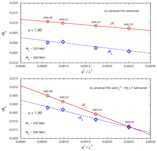
In order to study the FVEs in detail we consider four ensembles generated at the same values of and quark masses, but differing in the size of the lattice; these are the ensembles A40.40, A40.32, A40.24 and A40.20 (see Appendix A). The residual FVEs after the subtraction of the universal terms as in Eq. (96) are illustrated in the plots in Fig. 9 for and in the fully inclusive case, i.e. where the energy of the final-state photon is integrated over the full phase space. In this case , which corresponds to MeV and MeV, respectively. With a muon as the final state lepton, the contribution from photons with energy greater than about 20 MeV is negligible and hence the point-like approximation is valid. In the top plot the universal FV corrections have been subtracted and so we would expect the remaining effects to be of order and this is indeed what we see.
In the bottom plot of Fig. 9, in addition to subtracting the universal FVEs, we also subtract the contribution to the order corrections from the point-like contribution to , which can be found in Eq. (3.2) of Ref. Tantalo:2016vxk . We observe that this additional subtraction does not reduce the effects, underlining the expectation that these effects are indeed structure dependent.
It can be seen that after subtraction of the universal terms the residual structure-dependent FVEs are almost linear in , which implies that the FVEs of order are quite small; indeed they are too small to be resolved with the present statistics. Nevertheless, since the QEDL formulation of QED on a finite box, which is adopted in this work, violates locality Patella:2017fgk , we may expect that there are also FVEs of order Tantalo:2016vxk . We have checked explicitly that the addition of such a term in fitting the results shown in Fig. 9 changes the extrapolated value at infinite volume well within the statistical errors.
A more detailed description of the full analysis, including the continuum and chiral extrapolations, is given in the following section. As far as the FVEs are concerned, the central value is obtained by subtracting the universal terms and fitting the residual corrections to
| (97) |
where and are constant fitting parameters and is the energy of the charged lepton in the rest frame of the pseudoscalar (see Eq. (98) below). Such an ansatz is introduced to model the unknown dependance of on the ratio . For the four points in each of the plots of Fig. 9 takes the same value, but this is not true for all the ensembles used in the analysis. We estimate the uncertainty due to the use of the ansatz in Eq. (97) by repeating the same analysis, but on the data in which, in addition to subtracting the universal terms in Eq. (95), we also subtract the term , where is contribution to from a point-like meson Tantalo:2016vxk . Since depends on , the result obtained with this additional subtraction is a little different from that obtained with only the universal terms removed and we take the difference as an estimate of the residual FV uncertainty.
VI Results for charged pion and kaon decays into muons
We now insert the various ingredients described in the previous sections into the master formula in Eq. (29) for the decays and .
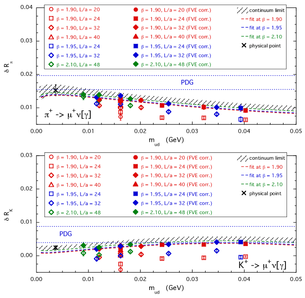
The results for the corrections and are shown in Fig. 10, where the “universal” FSEs up to order have been subtracted from the lattice data (see the empty symbols) and all photon energies (i.e. ) are included, since the experimental data on and decays are fully inclusive. As already pointed out in section I, structure dependent contributions to real photon emission should be included. According to the ChPT predictions of Ref. Cirigliano:2007ga , however, these contributions are negligible in for both kaon and pion decays into muons, while the same does not hold as well for decays into final-state electrons (see Ref. Carrasco:2015xwa ). This important conclusion needs to be explicitly validated by an ongoing dedicated lattice study of the real photon emission amplitudes in light and heavy P-meson leptonic decays.
The combined chiral, continuum and infinite-volume extrapolations are performed using the following SU(2)-inspired fitting function
| (98) | |||||
where and is the bare (twisted) mass (see Table 2 in Appendix A below), is the lepton energy in the P-meson rest frame, , , and are free parameters. In Eq. (98) the chiral coefficient is known for both pion and kaon decays from Ref. Bijnens:2006mk ; in QED the coefficients are
| (99) |
while in qQED they are
| (100) |
where is obtained from the chiral limit of the correction to (i.e. ). In Ref. Giusti:2017dmp we found .
Using Eq. (98) we have fitted the data for and using a -minimization procedure with an uncorrelated , obtaining values of always around . The uncertainties on the fitting parameters do not depend on the -value, because they are obtained using the bootstrap samplings of Ref. Carrasco:2014cwa (see Appendix A). This guarantees that all the correlations among the data points and among the fitting parameters are properly taken into account.
The quality of our fits is illustrated in Fig. 10. It can be seen that the residual SD FVEs are still visible in the data and well reproduced by our fitting ansatz in Eq. (98). Discretisation effects on the other hand, only play a minor role.
At the physical pion mass in the continuum and infinite-volume limits we obtain
| (101) | |||||
| (102) | |||||
where
-
•
indicates the uncertainty induced by the statistical Monte Carlo errors of the simulations and its propagation in the fitting procedure;
-
•
is the error coming from the uncertainties of the input parameters of the quark-mass analysis of Ref. Carrasco:2014cwa ;
-
•
is the difference between including or excluding the chiral logarithm in Eq. (98), i.e. taking or ;
- •
-
•
is the uncertainty coming from including () or excluding (setting ) the discretisation term proportional to in Eq. (98);
-
•
is our estimate of the uncertainty of the QED quenching. This is obtained using the ansatz (98) with the coefficient of the chiral log fixed either at the value (100), which corresponds to the qQED approximation, or at the value (99), which includes the effects of the up, down and strange sea-quark charges Bijnens:2006mk . The change both in and in is , which has been already added in the central values given by Eqs. (101) and (102). To be conservative, we use twice this value for our estimate of the qQED uncertainty.
Our results in Eqs. (101) - (102) can be compared with the ChPT predictions and obtained in Ref. Cirigliano:2011tm and adopted by the PDG PDG ; Rosner:2015wva . The difference is within one standard deviation for , while it is larger for . Note that the precision of our determination of is comparable to the one obtained in ChPT, while our determination of has a much better accuracy compared to that obtained using ChPT; the improvement in precision is a factor of about 2.2. We stress that the level of precision of our pion and kaon results depends crucially on the non-perturbative determination of the chirality mixing, carried out in section IV by including simultaneously QED at first order and QCD at all orders.
As already stressed, the correction and the QCD quantity separately depend on the prescription used for the separation between QED and QCD corrections Gasser:2010wz . Only the product is independent of the prescription and its value, multiplied by the relevant CKM matrix element, yields the P-meson decay rate. We remind the reader that our results (101) - (102) are given in the GRS prescription (see the dedicated discussion in sections II.2 and III) in which the renormalised couplings and quark masses in the full theory and in isosymmetric QCD coincide in the scheme at a scale of 2 GeV Gasser:2003hk . We remind the reader that, to the current level of precision, this GRS scheme can be considered equivalent to the FLAG scheme.
Taking the experimental values s-1 and s-1 from the PDG PDG and using our results (101) - (102), we obtain
| (103) | |||||
| (104) |
where the first error is the experimental uncertainty and the second is that from our theoretical calculations. The result for the pion in Eq. (103) agrees within the errors with the updated value MeV PDG , obtained by the PDG and based on the model-dependent ChPT estimate of the e.m. corrections from Ref. Cirigliano:2011tm . Our result for the kaon in Eq. (104) however, is larger than the corresponding PDG value MeV PDG , based on the ChPT calculation of Ref. Cirigliano:2011tm , by about standard deviations.
As anticipated in the Introduction and discussed in detail in Sec. III, we cannot use the result (103) to determine the CKM matrix element , since the pion decay constant was used by ETMC Carrasco:2014cwa to set the lattice scale in isosymmetric QCD and its value, MeV, was based on the determination of obtained from super-allowed -decays in Ref. Hardy:2014qxa . On the other hand, adopting the best lattice determination of the QCD kaon decay constant, MeV FLAG ; Dowdall:2013rya ; Carrasco:2014poa ; Bazavov:2017lyh 777The average value of quoted by FLAG FLAG includes the strong IB corrections. In order to obtain therefore, we have subtracted this correction which is given explicitly in Refs. Dowdall:2013rya ; Carrasco:2014poa ; Bazavov:2017lyh ., we find that Eq. (104) implies
| (105) |
which is a result with the excellent precision of .
Since the non-factorisable e.m. corrections to the mass RC (see the coefficient in Table 1) were not included in Ref. Giusti:2017dwk , we update our estimate of the ratio of the kaon and pion decay rates:
| (106) |
Using the pion and kaon experimental decay rates we get
| (107) |
Using the best lattice determination of the ratio of the QCD kaon and pion decay constants, FLAG ; Dowdall:2013rya ; Carrasco:2014poa ; Bazavov:2017lyh , we find
| (108) |
Taking the updated value from super-allowed nuclear beta decays Hardy:2016vhg , Eq. (108) yields the following value for the CKM element :
| (109) |
which agrees with our result (105) within the errors. Note that our result (109) agrees with the latest estimate , recently updated by the PDG PDG , but it improves the error by a factor of approximately 1.5.
Taking the values PDG and Hardy:2016vhg our result in Eq. (109) implies that the unitarity of the first-row of the CKM matrix is confirmed to better than the per-mille level
| (110) |
With the same value from super-allowed nuclear beta decays Hardy:2016vhg , our result (103) implies for the QCD pion decay constant (in the GRS prescription) the following value
| (111) |
which, as anticipated in Sec. III, agrees within the errors with the value MeV adopted in Ref. Carrasco:2014cwa to set the lattice scale in the isosymmetric QCD theory. This demonstrates the equivalence of the GRS and PDG schemes within the precision of our simulation.
In a recent paper Seng:2018yzq the hadronic contribution to the electroweak radiative corrections to neutron and super-allowed nuclear decays has been analyzed in terms of dispersion relations and neutrino scattering data. With respect to the result from Ref. Hardy:2016vhg a significant shift in the central value and a reduction of the uncertainty have been obtained, namely Seng:2018yzq . The impact of the new value of on our determinations of and is and MeV, i.e. well within the uncertainties shown in Eqs. (109) and (111), respectively. On the contrary, the first-row CKM unitarity (110) will be significantly modified into
| (112) |
which would imply a tension with unitarity. A confirmation of the new calculation of the radiative corrections made in Ref. Seng:2018yzq is therefore urgently called for.
Before closing this section, we comment briefly about the comparison between our result and the corresponding model-dependent ChPT prediction from Ref. Cirigliano:2011tm . The latter is obtained by adding a model-dependent QED correction of and a model-independent next-to-leading strong IB contribution equal to . Our result on the other hand, obtained in the GRS prescription, stems from a QED correction equal to and a strong IB term equal to (see also Ref. Giusti:2017xrv ). The difference between our result and the ChPT prediction of Ref. Cirigliano:2011tm appears to be mainly due to a different strong IB contribution. Thus, in the present study, we confirm for the strong IB term a discrepancy at the level of about 2 standard deviations, which was already observed at in Ref. deDivitiis:2013xla .
VII Conclusions
In this paper we have presented the details of the first lattice computation of the leading e.m. and strong IB corrections to the and leptonic decay rates, following a method recently proposed in Ref. Carrasco:2015xwa . This expands significantly on the discussion of Ref. Giusti:2017dwk , where the results and a brief outline of the calculation had been presented. The results were obtained using the gauge ensembles produced by the European Twisted Mass Collaboration with dynamical quarks. Systematics effects are evaluated and the impact of the quenched QED approximation is estimated.
The effective weak Hamiltonian in the W-regularisation scheme appropriate for this calculation is obtained from the bare lattice operators in two stages. First of all, the lattice operators are renormalised non-perturbatively in the RI′-MOM scheme at and to all orders in the strong coupling . Because of the breaking of chiral symmetry in the twisted mass formulation we have adopted this renormalisation includes the mixing with other four-fermion operators of different chirality. In the second step we perform the matching from the RI′-MOM scheme to the W-regularisation scheme perturbatively. By calculating and including the two-loop anomalous dimension at Brod:2008ss , the residual truncation error of this matching is of , reduced from in our earlier work Giusti:2017dwk ; Carrasco:2015xwa .
The evaluation of isospin breaking (IB) “corrections” raises the question of how QCD without these corrections is defined. Since IB corrections change hadronic masses and other physical quantities a prescription is needed to define QCD, whether isosymmetric or not, and in Sec. II and Appendix B we discuss this issue in detail. In particular, the correction and the QCD quantity separately depend on the prescription used for the definition of QCD Gasser:2010wz . Only the product is independent of the prescription and its value, multiplied by the relevant CKM matrix element, yields the P-meson decay rate. In this paper we chose to follow the conventionally used GRS prescription (see the dedicated discussion in sections II.2 and III) in which the renormalised couplings and quark masses in the full QCD+QED theory and in isosymmetric QCD coincide in the scheme at a scale of 2 GeV Gasser:2003hk . For future studies however, we advocate the use of “hadronic schemes” in which QCD is defined by requiring that a set of hadronic quantities (for example a set of hadronic masses) take their physical values in QCD and in QCD+QED.
The main results of the calculation are presented in Sec. VI together with a detailed discussion of their implications. In summary, after extrapolation of the data to the physical pion mass, and to the continuum and infinite-volume limits, the isospin-breaking corrections to the leptonic decay rates can be written in the form:
| (113) | |||||
| (114) | |||||
where is the leptonic decay rate at tree level in the GRS scheme (see Eqs. (101) and (102)). These results can be compared with the ChPT predictions and obtained in Ref. Cirigliano:2011tm and adopted by the PDG PDG ; Rosner:2015wva . The difference is within one standard deviation for , while it is larger for . We also underline that our result in Eq. (109), together with the value of determined in Ref. Hardy:2016vhg and from the PDG PDG , implies that the unitarity of the first row of the CKM matrix is satisfied at the per-mille level (see Eq. (110)).
Acknowledgments
We gratefully acknowledge the CPU time provided by the Partnership for Advanced Computing in Europe (PRACE) under the project Pra10-2693 “QED corrections to meson decay rates in Lattice QCD” and by CINECA under the specific initiative INFN-LQCD123 on the BG/Q system Fermi at CINECA (Italy). V.L., G.M. and S.S. thank MIUR (Italy) for partial support under the contract PRIN 2015. G.M. also acknowledges partial support from the European Research Council Ideas Advanced Grant n. 267985 “DaMeSyFla”. C.T.S. was partially supported by the UK Science and Technology Facilities Council (STFC) grant No. ST/P000711/1 and by an Emeritus Fellowship from the Leverhulme Trust. N.T. gratefully acknowledges the University of Rome Tor Vergata for the support granted to the project PLNUGAMMA.
Appendix A Details of the simulation
The gauge ensembles used in this work are those generated by ETMC with dynamical quarks and used in Ref. Carrasco:2014cwa to determine the up, down, strange and charm quark masses. We use the Iwasaki action Iwasaki:1985we for the gluons and the Wilson Twisted Mass Action Frezzotti:2000nk ; Frezzotti:2003xj ; Frezzotti:2003ni for the sea quarks. In the valence sector we adopt a non-unitary setup Frezzotti:2004wz in which the strange quark is regularized as an Osterwalder-Seiler fermion Osterwalder:1977pc , while the up and down quarks have the same action as the sea. Working at maximal twist such a setup guarantees an automatic -improvement Frezzotti:2003ni ; Frezzotti:2004wz .
We have performed simulations at three values of the inverse bare lattice coupling and at several different lattice volumes as shown in Table 2. We allow a separation of 20 trajectories between each of the analysed configurations. For the earlier investigation of finite-volume effects (FVEs) ETMC had produced three dedicated ensembles, A40.20, A40.24 and A40.32, which share the same quark masses and lattice spacing and differ only in the lattice size . To improve such an investigation, which is crucial in the present work, we have generated a further gauge ensemble, A40.40, at a larger value of the lattice size .
| ensemble | ||||||||||
|---|---|---|---|---|---|---|---|---|---|---|
| 317 (12) | 576 (22) | 5.7 | ||||||||
| 275 (10) | 568 (22) | 3.9 | ||||||||
| 316 (12) | 578 (22) | 4.5 | ||||||||
| 350 (13) | 586 (22) | 5.0 | ||||||||
| 322 (13) | 582 (23) | 3.5 | ||||||||
| 386 (15) | 599 (23) | 4.2 | ||||||||
| 442 (17) | 618 (14) | 4.8 | ||||||||
| 495 (19) | 639 (24) | 5.3 | ||||||||
| 330 (13) | 586 (23) | 3.0 | ||||||||
| 259 (9) | 546 (19) | 3.4 | ||||||||
| 302 (10) | 555 (19) | 4.0 | ||||||||
| 375 (13) | 578 (20) | 5.0 | ||||||||
| 436 (15) | 599 (21) | 5.8 | ||||||||
| 468 (16) | 613 (21) | 4.6 | ||||||||
| 223 (6) | 529 (14) | 3.4 | ||||||||
| 256 (7) | 535 (14) | 3.9 | ||||||||
| 312 (8) | 550 (14) | 4.7 |
At each lattice spacing, different values of the light sea-quark masses have been considered. The light valence and sea quark masses are always taken to be degenerate. The bare mass of the valence strange quark () is obtained, at each , using the physical strange mass and the mass RCs determined in Ref. Carrasco:2014cwa . There the “FLAG” hadronic scheme was adopted in which the pion and kaon masses in isosymmetric QCD are equal to MeV and MeV and the lattice scale is fixed by the value MeV for the physical pion decay constant. In the charm sector instead, the -meson mass was chosen to be equal to its experimental value MeV PDG . The values of the lattice spacing are found to be , , fm at , and , respectively.
The two valence quarks and in the P meson are regularized with opposite values of the Wilson -parameter () in order to guarantee that discretisation effects on the P meson mass are of order . The lepton is a free twisted-mass fermion with Wilson parameter and its mass is taken fixed at the physical muon value MeV PDG . The regularization of the (massless) neutrino is irrelevant and it is taken to be a free fermion field.
In this work we made use of the bootstrap samples generated for the input parameters of the quark mass analysis of Ref. Carrasco:2014cwa . There, eight branches of the analysis were adopted differing in:
-
•
the continuum extrapolation adopting for the matching of the lattice scale either the Sommer parameter or the mass of a fictitious P-meson made up of two valence strange(charm)-like quarks;
-
•
the chiral extrapolation performed with fitting functions chosen to be either a polynomial expansion or a Chiral Perturbation Theory (ChPT) Ansatz in the light-quark mass;
-
•
the choice between the methods M1 and M2, which differ by effects, used to determine the mass RC in the RI′-MOM scheme .
Appendix B Relating observables in the full theory and in QCD
In this appendix we provide the detailed derivation of the relation between observables calculated in the full theory (QCD+QED) and in QCD (in the absence of QED). We start by a discussion of the separation of the QCD action from that in the full theory.
B.1 Actions of the full theory and of QCD
The lattice action in the full theory given in Eq. (4) can be written as
| (115) |
where and the counterterm and the QED vertices are given by
| (116) | |||||
| (117) |
We now consider these terms in detail using Wilson fermions for illustration. The kinetic term for the quark with flavour , , is given by:
| (118) |
where is the quark field, while and are the QCD and QED gauge links, respectively. Specifically
| (119) |
where is the charge of the quark with flavour in units of the positron charge. The forward and backward derivatives are given by
| (120) | |||||
| (121) |
The leptonic action is given by
| (122) |
with being the lepton field. The renormalisation of the lepton masses is performed perturbatively, by requiring that the on-shell masses correspond to the physical ones.
In QCD the kinetic term only includes the gluon links so that for Wilson fermions
| (123) |
and the derivatives are defined in Eqs. (120) - (121) with the . Since for leptonic and semileptonic decays, leptonic spinors are present even in the absence of electromagnetism, it is also convenient to define the kinetic action for free leptons:
| (124) |
B.2 Relation between observables in the full theory and in QCD
Physical observables are determined from correlation functions evaluated from lattice computations in the full theory. For a generic observable evaluated in the full theory up to we write:
| (125) | |||||
where in the integrand is a multilocal composite operator. For a given choice of the strong coupling , the parameters of the action, the bare quark masses and the lattice spacing, are determined by imposing that a set of physical quantities take their experimental values as explained in Sec. II.1. Physical quantities other than those used for the calibration can now be determined unambiguously up to lattice artefacts, which are removed by taking the continuum limit.
In general, the determination of physical observables requires the processing of correlation functions of the form of Eq. (125). Hadronic masses, for example are obtained from the behaviour in the time separation of two interpolating operators and the determination of hadronic matrix elements may require the cancelation of interpolating operators at the source and/or sink using a combination of three- and two-point functions. The discussion in this appendix concerns the evaluation of a generic correlation function.
We now turn to the definition of correlation functions in QCD defined in a generic scheme. For a generic observable we define its value in QCD by:
| (126) |
where the bare quark masses and the lattice spacing are defined as discussed in Sec. II.2. The free QED action is included in the numerator and denominator of Eq. (126) since even without radiative corrections the physical quantities such as and studied in this paper are obtained by combining the results for hadronic matrix elements obtained from QCD simulations with leptonic spinors. Moreover, for other quantities, for example the long-distance contributions to the amplitude for the rare kaon decay , there are internal free lepton propagators even in the absence of isospin breaking Christ:2016eae .
Comparing Eqs. (125) and (126) we arrive at
| (127) |
where the subscript “conn” reminds that only connected Feynman diagrams contribute: .
There is one final subtlety which we must account for. We need to convert the results obtained from simulations in lattice units (i.e. in units of the lattice spacing) into values given in physical units such as MeV. Eq. (127) is also written in lattice units. Imagine that the observable has mass dimension and rewrite Eq. (127) with the lattice spacing included explicitly:
| (128) |
where, since we are working to first order in isospin breaking, in the second term on the right-hand side we do not need to distinguish between the lattice spacing in the full theory () and that obtained in QCD (). The quantity which we wish to determine, in physical units, is therefore given by
| (129) |
where . The three expectation values on the right-hand side of (129) are directly computed in QCD simulations.
Appendix C Non-perturbative renormalisation in the RI'-MOM scheme
In this paper, as explained in Sec. IV, we have renormalised the weak four-fermion operator non-perturbatively on the lattice to all orders in and up to first order in . In this appendix we describe the main steps of the non-perturbative renormalisation procedure at and we refer the reader to a forthcoming publication dicarlo for further details and results.
Given the amputated Green function, , of an operator computed in a given gauge between external states with momentum and a suitable projector on the relevant Dirac structure, , we define the projected Green function as
| (130) |
In the RI'-MOM scheme, the renormalisation constant (RC) is found by imposing the condition Martinelli:1994ty
| (131) |
where
| (132) |
The are the RCs of the external fields and the index runs over all external fields entering the expression of the composite operator . For the four-fermion operators considered in this work, the RCs and the projected Green functions are matrices, the latter with elements . In QCD+QED the RCs and depend both on the strong and the e.m. coupling constants.
Following the discussion of Sec. IV (see Eqs. (75) - (78)), we write the RCs of any composite operator, and in particular of the fields, bilinear and four-fermion operators, in the generic decomposition
| (133) | |||||
where and are the RCs of the operator in pure QCD and pure QED respectively and we have put
| (134) |
The first term, , in Eq. (134) represents the pure QED contribution to the RC at , whereas contains the non-factorisable QCD+QED correction.
In terms of the QCD renormalised operators , as those in Eq. (79), we define the QCD renormalised projected Green function , and expand it at first order in
| (135) | |||||
where we have used the RI'-MOM renormalisation condition applied in the pure QCD theory and defined
| (136) |
Using Eqs. (133) and (135), we can rewrite Eq. (131) at first order in as
| (137) |
which provides, in turn, the RI-MOM renormalisation condition at order
| (138) |
Using the expression of in Eq. (132) in terms of and the external fields RCs one also obtains
| (139) |
Thus, is expressed directly in terms of the contribution to the QCD renormalised projected Green function evaluated at .
In the following we describe a completely non-perturbative determination of the RCs to all orders in . We will assume that all the relevant RCs of fields and composite operators in pure QCD have been already determined, by following the standard RI'-MOM renormalisation procedure. With appropriate modifications to the kinematical conditions and projectors, the discussion can readily be adapted to similar schemes, such as the Symmetric Momentum subtraction one Sturm:2009kb .
In addition to the renormalisation of the four-fermion operator appearing in the Hamiltonian, the e.m. shift of the quark masses (see Sec. III.1) requires the knowledge of the RC of the pseudoscalar density deDivitiis:2013xla . We therefore start by discussing the non-perturbative renormalisation of quark bilinear operators.
C.1 Renormalisation of the quark field and bilinear operators
We start with the renormalisation of the quark fields. The e.m. corrections to a quark propagator can be represented schematically in the form
| (140) |
where the last two diagrams represent the mass and critical Wilson parameter counter-terms deDivitiis:2013xla .
The amputated one-particle irreducible two-point function is then given by
| (141) |
and the correction to the quark field RC in the RI'-MOM scheme is obtained, according to Eq. (138), as
| (142) |
The e.m. correction to the RC of a generic bilinear operator , where is one of the Dirac matrices (), is given by Eq. (139), which in this case reads
| (143) |
Two kinds of corrections contribute to the amputated Green function: either the QCD Green function is amputated with the e.m. corrections on the inverse propagators, or the correction to the Green function itself is amputated with QCD propagators. Thus we have
| (144) |
with
| (145) | |||||
where is the non-amputated Green function and is given diagrammatically by
| (146) |
In this work we have used an improved method to compute the first diagram in Eq. (146), as well as all the diagrams containing a photon propagator connecting different points. In this method, some of the sequential propagators introduced in Ref. Giusti:2017dmp are summed in order to reduce the number of inversions of the Dirac matrix. All details of the calculation will be given in the forthcoming publication dicarlo .
Before closing this subsection, we stress that in the calculation of and its e.m. correction , the Goldstone pole contamination has been taken into account and subtracted. In pure QCD, at each and for each combination of valence quark masses, and , the amputated Green function has been fitted to the ansatz
| (147) |
where is the mass of the pseudoscalar meson composed of valence quarks of mass and . When including QED in the calculation, Eq. (147) has to be modified to take into account the e.m. correction to the meson mass. By considering the ansatz in Eq. (147) in QCD+QED and expanding it in terms of one finds
| (148) |
where is the correction to evaluated in Ref. Giusti:2017dmp . Note, in particular, that also receives the contribution of a double pole. In Eq. (148) only the coefficients , , need to be fitted, since the values of and are already obtained from the QCD fit in Eq. (147).
C.2 Renormalisation of the four-fermions operators
We conclude this section by describing the calculation of the RCs of the complete basis of four-fermion operators (), in the RI'-MOM scheme. In this case, the renormalisation condition (139) for the renormalisation matrix at reads:
| (149) |
where is only e.m. and can be computed in perturbation theory. We remind the reader that this term is omitted in the actual calculation since its contribution cancels out in the difference .
In Eq. (149) is a matrix expressed by
| (150) |
As in the case of bilinear operators, the correction to the amputated Green function gets two kind of contributions,
| (151) | |||||
and in this case is given by
The fermionic lines on the left-hand side of the diagrams in Eq. (C.2) represent the ingoing and outgoing light quarks. On the right-hand side, the external charged anti-lepton and the neutrino propagators are drawn for illustration but not actually included in the calculation. For this reason their amputation is neglected in Eq. (151). The lepton self-energy is not reported in Eq. (C.2) since its contribution cancels out in the amputation.
Appendix D Matching, chirality mixing and fermion operators in the twisted mass regularisation
In the main text and in Appendix C we have described the renormalisation of the relevant operators in the physical basis. This discussion is valid for a generic Wilson-like fermion regularisation. In this appendix we address instead some important aspects peculiar to the twisted mass fermions used in our numerical calculation. We derive, in particular, the relations between RCs in the so-called physical and twisted basis, for the bilinear and four-fermion operators considered in this work.
The relevant observation is that the lattice action for twisted mass fermions at maximal twist in the twisted basis only differs from the standard Wilson fermion lattice action for the twisted rotation of the fermion mass term. The two actions become identical in the chiral limit. It then follows that, in any mass-independent renormalisation scheme, the RCs for twisted mass operators in the twisted basis are the same as those of the corresponding operators with standard Wilson fermions. It is customary to denote these RCs, for a generic operator , as . They are valid for both standard Wilson and twisted mass operators in the twisted basis and differ, in general, from the RCs for twisted mass operators in the physical basis, that we denote here as .
At maximal twist the rotation from the twisted to the physical basis for both quark and lepton fields is given by
| (153) |
where and are the quark and lepton fields in the physical basis and and are the corresponding -parameters. In our simulations we use opposite values of the -parameter for the two valence quarks, (). The quark and lepton bilinears then transform as
| (154) | |||||
From Eqs. (D) one readily derives the relations between the quark vector and axial vector current in the two basis,
| (155) |
which, in turn, determine the relation between the RCs in the two basis
| (156) |
where denotes the generic renormalised operator. One then sees from Eq. (156) that the RC of the vector current in the physical basis, with , is simply the RC of the axial current in the twisted basis, which in turn is just computed with Wilson fermions in the chiral limit. Analogously, in the physical basis, with , corresponds to computed with Wilson fermions in the chiral limit.
From the transformations (D) one can also derive the relations between the four-fermion operators of Eq. (24) and (73) in the physical and twisted basis
| (157) | ||||
We can then obtain the relation between the renormalisation matrix in the physical basis, , and the corresponding matrix for standard Wilson fermions. In particular, for the weak operator one finds
| (158) | |||||
with . Therefore
| (159) |
Eq. (159) shows in particular that the mixing coefficients for the operators are proportional to . Thus, we can eliminate the mixing with these operators by simply averaging the numerical results over the two possible values .
In order to illustrate the above point, using the results of Ref. Carrasco:2015xwa obtained in perturbation theory at order , the coefficients are explicitly given in the physical basis by
| (160) |
References
- (1) N. Cabibbo, Phys. Rev. Lett. 10 (1963) 531. M. Kobayashi and T. Maskawa, Prog. Theor. Phys. 49 (1973) 652.
- (2) D. Giusti, V. Lubicz, G. Martinelli, C. T. Sachrajda, F. Sanfilippo, S. Simula, N. Tantalo and C. Tarantino, Phys. Rev. Lett. 120 (2018) no.7, 072001 [arXiv:1711.06537 [hep-lat]].
- (3) S. Aoki et al. [Flavour Lattice Averaging Group], arXiv:1902.08191 [hep-lat].
- (4) G. M. de Divitiis et al., Phys. Rev. D 87 (2013) no.11, 114505 [arXiv:1303.4896 [hep-lat]].
- (5) S. Borsanyi et al., Science 347 (2015) 1452 [arXiv:1406.4088 [hep-lat]].
- (6) P. Boyle, V. Gülpers, J. Harrison, A. Jüttner, C. Lehner, A. Portelli and C. T. Sachrajda, JHEP 1709 (2017) 153 [arXiv:1706.05293 [hep-lat]].
- (7) M. Hansen, B. Lucini, A. Patella and N. Tantalo, JHEP 1805 (2018) 146 [arXiv:1802.05474 [hep-lat]].
- (8) D. Giusti, V. Lubicz, C. Tarantino, G. Martinelli, S. Sanfilippo, S. Simula and N. Tantalo, Phys. Rev. D 95 (2017) no.11, 114504 [arXiv:1704.06561 [hep-lat]].
- (9) G. M. de Divitiis et al., JHEP 1204 (2012) 124 [arXiv:1110.6294 [hep-lat]].
- (10) F. Bloch and A. Nordsieck, Phys. Rev. 52 (1937) 54.
- (11) N. Carrasco, V. Lubicz, G. Martinelli, C. T. Sachrajda, N. Tantalo, C. Tarantino and M. Testa, Phys. Rev. D 91 (2015) no.7, 074506 [arXiv:1502.00257 [hep-lat]].
- (12) M. Hayakawa and S. Uno, Prog. Theor. Phys. 120 (2008) 413 [arXiv:0804.2044 [hep-ph]].
- (13) A. Patella, PoS LATTICE 2016 (2017) 020 [arXiv:1702.03857 [hep-lat]].
- (14) V. Lubicz, G. Martinelli, C. T. Sachrajda, F. Sanfilippo, S. Simula and N. Tantalo, Phys. Rev. D 95 (2017) no.3, 034504 [arXiv:1611.08497 [hep-lat]].
- (15) R. Baron et al. [ETM Coll.], JHEP 1006 (2010) 111 [arXiv:1004.5284 [hep-lat]].
- (16) R. Baron et al. [ETM Collaboration], PoS LATTICE 2010 (2010) 123 [arXiv:1101.0518 [hep-lat]].
- (17) V. Cirigliano and I. Rosell, JHEP 0710 (2007) 005 [arXiv:0707.4464 [hep-ph]].
- (18) A. Sirlin, Nucl. Phys. B 196 (1982) 83.
- (19) J. Gasser, A. Rusetsky, I. Scimemi, Eur. Phys. J. C32 (2003) 97-114. [hep-ph/0305260].
- (20) M. Tanabashi et al. [Particle Data Group], Phys. Rev. D 98 (2018) no.3, 030001.
- (21) J. Hardy and I. S. Towner, PoS CKM 2016 (2016) 028.
- (22) D. Giusti, V. Lubicz, G. Martinelli, C. Sachrajda, F. Sanfilippo, S. Simula and N. Tantalo, PoS LATTICE 2018 (2019) 266 [arXiv:1811.06364 [hep-lat]].
- (23) M. Bochicchio, L. Maiani, G. Martinelli, G. C. Rossi and M. Testa, Nucl. Phys. B 262 (1985) 331.
- (24) B. Lucini, A. Patella, A. Ramos and N. Tantalo, JHEP 1602 (2016) 076 [arXiv:1509.01636 [hep-th]].
- (25) V. Cirigliano and H. Neufeld, Phys. Lett. B 700 (2011) 7 [arXiv:1102.0563 [hep-ph]].
- (26) J. L. Rosner, S. Stone and R. S. Van de Water, Submitted to: Particle Data Book [arXiv:1509.02220 [hep-ph]].
- (27) J. Gasser and G. R. S. Zarnauskas, Phys. Lett. B 693 (2010) 122 [arXiv:1008.3479 [hep-ph]].
- (28) N. Carrasco et al. [ETM Coll.], Nucl. Phys. B 887 (2014) 19 [arXiv:1403.4504 [hep-lat]].
- (29) M. Di Carlo et al., in preparation.
- (30) G. Martinelli and Y. C. Zhang, Phys. Lett. 123B (1983) 433.
- (31) S. Aoki, K. i. Nagai, Y. Taniguchi and A. Ukawa, Phys. Rev. D 58 (1998) 074505 [hep-lat/9802034].
- (32) D. Giusti, V. Lubicz, G. Martinelli, F. Sanfilippo and S. Simula, JHEP 1710 (2017) 157 [arXiv:1707.03019 [hep-lat]].
- (33) P. F. Bedaque, Phys. Lett. B 593 (2004) 82 [nucl-th/0402051].
- (34) G. M. de Divitiis, R. Petronzio and N. Tantalo, Phys. Lett. B 595 (2004) 408 [hep-lat/0405002].
- (35) G. Martinelli, C. Pittori, C. T. Sachrajda, M. Testa and A. Vladikas, Nucl. Phys. B 445 (1995) 81 [hep-lat/9411010].
- (36) A. J. Buras, M. Jamin and M. E. Lautenbacher, Nucl. Phys. B 408, 209 (1993) [hep-ph/9303284].
- (37) M. Ciuchini, E. Franco, G. Martinelli and L. Reina, Nucl. Phys. B 415, 403 (1994) [hep-ph/9304257].
- (38) J. Brod and M. Gorbahn, Phys. Rev. D 78 (2008) 034006 [arXiv:0805.4119 [hep-ph]].
- (39) N. Tantalo, V. Lubicz, G. Martinelli, C. T. Sachrajda, F. Sanfilippo and S. Simula, arXiv:1612.00199 [hep-lat].
- (40) J. Bijnens and N. Danielsson, Phys. Rev. D 75 (2007) 014505 [hep-lat/0610127].
- (41) R. Frezzotti and G. C. Rossi, Nucl. Phys. Proc. Suppl. 128 (2004) 193 [hep-lat/0311008].
- (42) J. C. Hardy and I. S. Towner, Phys. Rev. C 91 (2015) no.2, 025501 [arXiv:1411.5987 [nucl-ex]].
- (43) R. J. Dowdall, C. T. H. Davies, G. P. Lepage and C. McNeile, Phys. Rev. D 88 (2013) 074504 [arXiv:1303.1670 [hep-lat]].
- (44) N. Carrasco et al., Phys. Rev. D 91 (2015) no.5, 054507 [arXiv:1411.7908 [hep-lat]].
- (45) A. Bazavov et al., Phys. Rev. D 98 (2018) no.7, 074512 [arXiv:1712.09262 [hep-lat]].
- (46) C. Y. Seng, M. Gorchtein, H. H. Patel and M. J. Ramsey-Musolf, Phys. Rev. Lett. 121 (2018) no.24, 241804 [arXiv:1807.10197 [hep-ph]].
- (47) D. Giusti, V. Lubicz, G. Martinelli, F. Sanfilippo, S. Simula, N. Tantalo and C. Tarantino, EPJ Web Conf. 175 (2018) 06002 [arXiv:1710.06633 [hep-lat]].
- (48) Y. Iwasaki, Nucl. Phys. B 258 (1985) 141.
- (49) R. Frezzotti et al. [Alpha Collaboration], JHEP 0108 (2001) 058 [hep-lat/0101001].
- (50) R. Frezzotti and G. C. Rossi, JHEP 0408 (2004) 007 [hep-lat/0306014].
- (51) R. Frezzotti and G. C. Rossi, JHEP 0410 (2004) 070 [hep-lat/0407002].
- (52) K. Osterwalder and E. Seiler, Annals Phys. 110 (1978) 440.
- (53) N. H. Christ et al. [RBC and UKQCD Collaborations], Phys. Rev. D 93 (2016) no.11, 114517 [arXiv:1605.04442 [hep-lat]].
- (54) C. Sturm, Y. Aoki, N. H. Christ, T. Izubuchi, C. T. C. Sachrajda and A. Soni, Phys. Rev. D 80 (2009) 014501 doi:10.1103/PhysRevD.80.014501 [arXiv:0901.2599 [hep-ph]].