Some ordering properties of highest and lowest order statistics with exponentiated Gumble type-II distributed components

Abstract

In this paper, we have studied the stochastic comparisons of highest and lowest order statistics of exponentiated Gumble type-II distribution with three parameters. We have compared both the statistics by using three different stochastic ordering. First, we consider a system with different scale and outer shape parameters and then we study the usual stochastic ordering of the lowest and highest order statistics in the sense of multivariate chain majorization. In addition, we construct two examples to support our results. Second, by using the vector majorization technique, we study the usual stochastic ordering, the reversed failure rate ordering and the likelihood ratio ordering with respect to different outer shape parameters, next, by varying the inner shape parameter, we discuss the usual stochastic order of the lowest order statistics and we have shown that the highest order statistics are not comparable in the usual stochastic ordering by an example.

1 Introduction

In nature parallel and series systems are very common phenomena. Parallel and series system are $1$-out-of-$n$ and $n$-out-of-$n$ system, respectively. A $k$-out-of-$n$ systems is a system which functions if and only if at least $k$ out of its $n$ components function. These systems come under a particular class of order statistics. It is well known that the order statistics plays an important role in statistics, applied probability, reliability theory, actuarial science, auction theory, hydrology, and many other areas.

Throughout this paper, we discuss various results for the parallel and series systems where the components of the system come from the independent exponentiated Gumble type-II distributed random variables. The exponentiated Gumbel type-2 distribution, studied by Okorie et al.[1] A random variable $X$ is said to have exponentiated Gumble type-II distribution (in short we use $\textquoteleft EG_{2}$’ throughout this paper) if its cumulative distribution function (cdf) is

$$F(x)=1-\left(1-e^{-\theta x^{-\phi}}\right)^{\alpha},\hskip 22.76228ptx>0;\hskip 7.11317pt\theta,\phi,\alpha>0.$$ (1)

Here $\theta$ is scale parameter and $\phi,\alpha$ are shape parameters. We call $\alpha$ as outer shape parameter and $\phi$ as inner shape parameter. We use the notation $X\sim EG_{2}(\theta,\phi,\alpha)$ if $X$ has the cumulative distribution function in (1). It has wide applications in reliability, hydrology, and in many other areas due to its simple mathematical form. For more details such as theory, methods, applications about this distribution, interested reader may refer to Okorie et al.[1] This $EG_{2}$ distribution is a generalization of some standard distributions such as the Gumbel type-2 distribution, Exponentiated Fréchet (EF) distribution, and Fréchet distribution when $\alpha=1,\theta=1$, and $\alpha,\theta=1$, respectively and for $y=x^{-\phi}$ it becomes Exponentiated Exponential (EE) distribution, see [1].

Let $X_{1},X_{2},.......,X_{n}$ be a set independently distributed random variables and $X_{n:n}=max\left\{X_{1},X_{2},.......,X_{n}\right\},\hskip 8.5359ptX_{1:n}=min\left\{X_{1},X_{2},.......,X_{n}\right\}$. $X_{1:n}$ is known as $1^{st}$ (lowest) order statistic which represents a series system and $X_{n:n}$ is known as $n^{th}$ (highest) order statistic which represents a parallel system, for more detail informations regarding order statistics see, Shaked M. et al.[2] Various discussions on order statistics in terms of stochastic comparisons are already available where the component variables follow Generalized Exponential[3], Exponential Weibull[4], Exponentiated Scale model[5] , Fréchet[6] distributions, etc. The comparisons include usual stochastic order, failure rate order, reversed failure rate order, likelihood ratio order, dispersive order, etc. For further details on stochastic comparisons, one may refer to [[7],[8],[9],[10]]. Some results of [3] are very much useful for developing our paper.

The aim of this paper is to present stochastic, likelihood ratio, and reversed order failure ordering for parallel, series systems having $EG_{2}$ distributed components. Now, let $X_{1},.....,X_{n}$ be independent random variables and each $X_{i}$’s follows $EG_{2}$ distributions i.e., $X_{i}\sim EG_{2}(\theta_{i},\phi_{i},\alpha_{i}),\hskip 5.69046pti=1,2,....,n$. Furthermore, let $X^{*}_{1},.....,X^{*}_{n}$ another set of independent random variables such that $X^{*}_{i}\sim EG_{2}(\theta_{i}^{*},\phi_{i}^{*},\alpha_{i}^{*}),\hskip 5.69046pti=1,2,....,n$. First, we discuss the stochastic order for the highest and lowest order statistics in the sense of multivariate majorization when, $\phi_{1}=\cdotp\cdotp\cdotp\cdotp\cdotp=\phi_{n}=\phi^{*}_{1}=\cdotp\cdotp\cdotp\cdotp\cdotp=\phi^{*}_{n}$ and the matrix of different parameters such as $\theta_{i},\alpha_{i},\theta^{*}_{i},\alpha^{*}_{i},\hskip 5.69046pti=1,2,....,n,$ change to another matrix. Second, when $\theta_{i}=\theta_{j}=\theta^{*}_{i}=\theta^{*}_{j}$, $\phi_{i}=\phi_{j}=\phi^{*}_{i}=\phi^{*}_{j},$ $i,j=1,2,....,n,$ and $(\alpha_{1},\cdotp\cdotp\cdotp\cdotp\cdotp\alpha_{n})\succeq^{m}(\alpha^{*}_{1},\cdotp\cdotp\cdotp\cdotp\cdotp\alpha^{*}_{n})$, we discuss the usual stochastic order for $X_{1:n}$, the reversed failure rate order for $X_{n:n}$ and we put a sufficient condition for the likelihood ratio order for the lowest order statistics. Finally, when $\theta_{i}=\theta_{j}=\theta^{*}_{i}=\theta^{*}_{j}$, $\alpha_{i}=\alpha_{j}=\alpha^{*}_{i}=\alpha^{*}_{j},$ $i,j=1,2,....,n,$ and $(\phi_{1},\cdotp\cdotp\cdotp\cdotp\cdotp\phi_{n})\succeq^{m}(\phi^{*}_{1},\cdotp\cdotp\cdotp\cdotp\cdotp\phi^{*}_{n}),$ we discuss the usual stochastic order only.

The road-map of our discussion for this paper is as follows.

In Section 2 some basic useful definitions, lemmas, and theorems are given which we have used throughout this paper. Section 3 which has two subsections, in first subsection we deal with the concept of multivariate majorization and achieve stochastic ordering only, and in the second subsection, we work with the concept of vector majorization technique for some ordering results between lowest and highest order statistics.

2 Preliminaries

In this section, we present some important definitions of some well-known facts together with some results that are most pertinent to developments in Section-3. We use the notation $\mathbb{R}$=$(-\infty,+\infty),$ $\mathbb{R}_{+}$=$[0,+\infty),$ and $\textquoteleft\log$’ for usual logarithm base $e,$ throughout this paper.

Let $X,Y$ be two non-negative continuous univariate random variables having following characteristics

• Cumulative distribution functions: $F(x)$,   $G(x)$.

• Reliability functions: $\overline{F}(x)=1-F(x)$,    $\overline{G}(x)=1-G(x)$.

• Probability density functions: $f(x)$,    $g(x)$.

• Failure rate functions: $r(x)=\dfrac{f(x)}{\overline{F}(x)},\hskip 5.69046pts(x)=\dfrac{g(x)}{\overline{G}(x)}$.

• Reversed failure rate functions: $\tilde{r}(x)=\dfrac{f(x)}{F(x)},\hskip 5.69046pt\tilde{s}(x)=\dfrac{g(x)}{G(x)}$.

Definition 2.1.

(Stochastic Order)
Let $X,Y$ be two random variables.

1. $X$ is smaller than $Y$ in the usual stochastic order denoted by, $X\leq_{st}Y$ iff $\overline{F}(x)\leq\overline{G}(x)$   $\forall$ $x\in\mathbb{R}$.

2. $X$ is said to be greater than $Y$ in the usual stochastic order denoted by, $Y\leq_{st}X$ iff $F(x)\leq G(x)$   $\forall$ $x\in\mathbb{R}$

3. $X$ is said to be smaller than $Y$ in failure rate order denoted by, $X\leq_{fr}Y$ iff $s(x)\leq r(x),\hskip 5.69046ptx\in\mathbb{R},$ or if $\dfrac{\overline{G}(x)}{\overline{F}(x)}$ is non-decreasing in $x$.

4. $X$ is smaller than $Y$ in reversed failure rate order denoted by, $X\leq_{rf}Y$ iff $\tilde{r}(x)\leq\tilde{s}(x),\hskip 5.69046ptx\in\mathbb{R},$ or if $\dfrac{G(x)}{F(x)}$ is non-decreasing in $x$.

5. $X$ is smaller than $Y$ in likelihood ratio order denoted by, $X\leq_{lr}Y$ if $\dfrac{g(x)}{f(x)}$ is non-decreasing in $x$.

The well-known relation between the above definitions is give by

$X\leq_{lr}Y\Longrightarrow X\leq_{fr}Y(X\leq_{rf}Y)\Longrightarrow X\leq_{st}Y$

Definition 2.2.

(Majorization)
Let $\textbf{y}=(y_{1},y_{2},...,y_{n})$ with the order components, $y_{(n)}\leq.....\leq y_{(1)}$ and $\textbf{x}=(x_{1},x_{2},.....,x_{n})$ with the order components $x_{(n)}\leq...\leq x_{(1)}$, be two real vectors from $\mathbb{R}^{n}$. Then we say y majorizes x if

$$\sum_{i=1}^{k}y_{i}\leq\sum_{i=1}^{k}x_{i}$$

$k=1,2,...,n-1,$ and $\sum_{i=1}^{n}y_{i}=\sum_{i=1}^{n}x_{i}.$ It is denoted by $\textbf{y}\succeq^{m}\textbf{x}$.

Definition 2.3.

Let $\textbf{y}=(y_{1},.....,y_{n})$ and $\textbf{x}=(x_{1},.....,x_{n})$ be two vectors from $\mathbb{R}^{n}$. A real valued function $\sigma(\textbf{y}):\mathbb{R}^{n}\rightarrow\mathbb{R}$ is said to be Schur-convex and Schur-concave if $\sigma(\textbf{y})\geq\sigma(\textbf{x})$ and $\sigma(\textbf{y})\leq\sigma(\textbf{x}),\hskip 5.69046pt\forall\textbf{y}\succeq^{m}\textbf{x}$, respectively.

The theorem, stated bellow is very useful for our results.

Theorem 2.4.

(Marshall et al., p.84, [12]): Let $I\subset\mathbb{R}$ be an open interval and let $\sigma:I^{n}\rightarrow\mathbb{R}$ be continuously differentiable function. The if and only if (iff) conditions for $\sigma$ to be Schur-convex(Schur-concave) on $I^{n}$ are $\sigma$ is symmetric on $I^{n}$ and, for all $i\neq j$

$(z_{i}-z_{j})\left(\dfrac{\partial\sigma}{\partial z_{i}}(\textbf{z})-\dfrac{\partial\sigma}{\partial z_{j}}(\textbf{z})\right)\geq 0\hskip 2.84544pt(\leq 0)$

for all $\textbf{z}\in I^{n}$. Where, $\dfrac{\partial\sigma}{\partial z_{i}}$ is partial derivative of $\sigma$ with respect to the $i^{th}$ component of z.

A square matrix $\Pi$ is said to be a permutation matrix if each row and column has a single unit, and all other entries are zero. We can always find $n!$ such matrices by interchanging rows (or columns) of the identity matrix of order $n$. Let $P=(p_{ij})$ be a matrix of order $n$, $P$ is said to be doubly stochastic if $p_{ij}\geq 0$ and $\sum_{i=1}^{n}p_{ij}=1=\sum_{j=1}^{n}p_{ij}$ for $i,j=1,2,....,n$. The $T$-transform matrix has the following form

$T_{w}=wI_{n}+(1-w)\Pi_{n}$,

where $w\in[0,1]$, $I_{n}$ is the $n\times n$ identity matrix and $\Pi_{n}$ is a permutation matrix of order $n$ that just interchanges two coordinates. One impotent fact about $T$-transformation matrices is that the product of a finite number of $T$-transformation matrices with the same structure is also $T$-transformation matrix and the resulting matrix has the same structure as the elements. But it may not hold for $T$-transformation matrices with different structures.

Now, in the next definition we various types of multivariate majorization [12].

Definition 2.5.

Let $A=\{a_{ij}\},B=\{b_{ij}\}$ be two merices of size $m\times n$ such that $a^{R}_{1},....a^{R}_{m}$ and $b^{R}_{1},....,b^{R}_{m}$ are the rows of $A$ and $B$ respectively, then:

1. $B$ is said to be chain majorized by $A$, denoted by $A\gg B$ if there exists a finite set of $T$-transformation matrices $T_{w_{1}},....,T_{w_{k}}$ of size $n\times n$ such that $B=AT_{w_{1}}.....T_{w_{k}}$;

2. $B$ is said to be majorized by $A$, denoted by $A>B$ if there exists an doubly stochastic matrix $P$ of size $n\times n$ such that $B=AP$;

3. $B$ is said to be row majorized by $A$, denoted by $A>^{row}B$ if $a^{R}_{i}\succeq^{m}b^{R}_{i}$ for $i=1,2,....,m$.

A well known implementation of these above forms of multivariate majorization is that

$A\gg B\implies A>B\implies A>^{row}B$.

Interested readers may refer to look at Chapter. 15 of Marshall et al.[12] for more details.

To prove our main results in next section we shall use the following theorems. Let us consider two set $\mathcal{S}_{n}$ and $\mathcal{T}_{n}$ defined as follows

$$\mathcal{S}_{n}=\left\{\begin{bmatrix}x_{1},\dots,x_{n}\\ y_{1},\dots,y_{n}\end{bmatrix}:(x_{i}-x_{j})(y_{i}-y_{j})\leq 0,and\hskip 8.5359ptx_{i}>0,y_{i}>0,\hskip 8.5359pti,j=1,...,n\right\},$$

and

$$\mathcal{T}_{n}=\left\{\begin{bmatrix}x_{1},\dots,x_{n}\\ y_{1},\dots,y_{n}\end{bmatrix}:(x_{i}-x_{j})(y_{i}-y_{j})\leq 0,and\hskip 8.5359ptx_{i}\geq 1,y_{i}>0,\hskip 8.5359pti,j=1,...,n\right\}.$$

Theorem 2.6.

A differentiable function $\psi:\mathbb{R}_{+}^{4}\rightarrow\mathbb{R}_{+}$ satisfies

$\psi(A)\leq(\geq)\psi(B)$ for all $A,B$ such that $A\in\mathcal{S}_{2}(\mathcal{T}_{2})$, and $A\gg B$ if and only if

1. $\psi(A)=\psi(\Pi A)$ for all permutation matrices $\Pi$, and for all $A\in\mathcal{S}_{2}(\mathcal{T}_{2})$;

2. $\sum_{i=1}^{2}(a_{ik}-a_{ij})(\psi_{ik}(A)-\psi_{ij}(A))\leq(\geq)0$ for all $j,k=1,2$ and for all $A\in\mathcal{S}_{2}(\mathcal{T}_{2})$, where $\psi_{ij}(A)=\dfrac{\partial\psi(A)}{\partial a_{ij}}.$

Proof.

Proof of this theorem can be find in Chapter 15, p.621 of Marshall et al.[12] ∎

Lemma 2.7.

Let the function $\eta:(0,\infty)\times(0,1)\rightarrow(-\infty,0)$ be defined as

$\eta(\alpha,u)=\dfrac{u^{\alpha}\log u}{1-u^{\alpha}}.$

Then,

1. $\eta(\alpha,u)$ is increasing with respect to $\alpha$ for each $0<u<1$;

2. $\eta(\alpha,u)$ is decreasing with respect to $u$ for each $\alpha>0$.

Proof.

Proof of this lemma is similar to the proof of the Lemma-2 in [3]. ∎

Lemma 2.8.

Let the function $\gamma:(0,\infty)\times(0,1)\rightarrow(0,\infty)$ be defined as

$\gamma(\alpha,u)=\dfrac{\alpha(1-u)u^{\alpha-1}}{1-u^{\alpha}}$.

Then,

1. $\gamma(\alpha,u)$ is decreasing with respect to $\alpha$ for each $0<u<1$;

2. $\gamma(\alpha,u)$ is decreasing with respect to $u$ for each $0<\alpha\leq 1;$

3. $\gamma(\alpha,u)$ is increasing with respect to $u$ for each $\alpha\geq 1$.

Proof.

Proof of this lemma is similar to the proof of the Lemma-3 in [3]. ∎

Lemma 2.9.

Let the function $\varphi(\alpha,u):(0,\infty)\times(0,1)\rightarrow(0,\infty)$ be defined as

$\varphi(\alpha,u)=\dfrac{\alpha u^{\alpha-1}}{1-u^{\alpha}}.$

Then $\varphi(\alpha,u)$ is convex in $\alpha$ for any $0<u<1.$

Proof.

Proof of this lemma is similar to the proof of the Lemma-7 in [3]. ∎

3 Main results

3.1 Results based on multivariate chain majorization

Let $X_{1},.....,X_{n}$ be a set of independent random variables and each $X_{i}$ follows $EG_{2}$ distributions i.e., $X_{i}\sim EG_{2}(\theta_{i},\phi_{i},\alpha_{i}),i=1,2,....,n$. Furthermore, let $X^{*}_{1},.....,X^{*}_{n}$ be another set of independent random variables such that $X^{*}_{i}\sim EG_{2}(\theta_{i}^{*},\phi_{i}^{*},\alpha_{i}^{*}),$ $i=1,2,....,n$. Assume $\phi_{1}=\cdotp\cdotp\cdotp\cdotp\cdotp\phi_{n}=\phi^{*}_{1}=\cdotp\cdotp\cdotp\cdotp\cdotp=\phi^{*}_{n}$. Here we deal with two systems (parallel, series) with independent $EG_{2}$ components having different scale and outer shape parameters i.e., different $\theta_{i}$’s, $\alpha_{i}$’s for $i=1,2,....,n.$

The next theorem discusses the usual stochastic ordering of lowest order statistics.

Theorem 3.1.

Let $X_{1},X_{2}$ and $X^{*}_{1},X^{*}_{2}$ be two pairs of non-negative independent random variables such that $X_{i}\sim EG_{2}(\theta_{i},\phi,\alpha_{i}),$ and $X^{*}_{i}\sim EG_{2}(\theta_{i}^{*},\phi,\alpha_{i}^{*})$ for $i=1,2$. Then, if $\begin{bmatrix}\alpha_{1}&\alpha_{2}\\ \theta_{1}&\theta_{2}\\ \end{bmatrix}$ $\in\mathcal{S}_{2}$ we have

$\begin{bmatrix}\alpha_{1}&\alpha_{2}\\ \theta_{1}&\theta_{2}\\ \end{bmatrix}$$\gg$ $\begin{bmatrix}\alpha^{*}_{1}&\alpha^{*}_{2}\\ \theta^{*}_{1}&\theta^{*}_{2}\\ \end{bmatrix}$$\implies X^{*}_{1:2}\geq_{st}X_{1:2}.$

Proof.

The reliability function of $X_{1:2}$ is given by, for $x>0$

$$\bar{F}_{X_{1:2}}(x)=\prod_{i=1}^{2}\left(1-e^{-\theta_{i}x^{-\phi}}\right)^{\alpha_{i}},\theta_{i},\phi,\alpha_{i}>0,\hskip 5.69046pti=1,2.$$

It is easy to prove that the function $\bar{F}_{X_{1:2}}(x)$ is permutation invariant with respect to $(\theta_{i},\alpha_{i}),i=1,2.$ So, the condition (1) of Theorem 2.6 is satisfied. Next, we need to show that the condition (2) of Theorem 2.6 also satisfies. Now, consider $\boldsymbol{\theta}=(\theta_{1},\theta_{2})$ and $\boldsymbol{\alpha}=(\alpha_{1},\alpha_{2})$ and let us define a function

$$G(\boldsymbol{\theta},\boldsymbol{\alpha})=G_{1}(\boldsymbol{\theta},\boldsymbol{\alpha})+G_{2}(\boldsymbol{\theta},\boldsymbol{\alpha})$$ (2)

Where,

$$G_{1}(\boldsymbol{\theta},\boldsymbol{\alpha})=(\alpha_{1}-\alpha_{2})\left(\dfrac{\partial\bar{F}_{X_{1:2}}(x)}{\partial\alpha_{1}}-\dfrac{\partial\bar{F}_{X_{1:2}}(x)}{\partial\alpha_{2}}\right),$$

$$G_{2}(\boldsymbol{\theta},\boldsymbol{\alpha})=(\theta_{1}-\theta_{2})\left(\dfrac{\partial\bar{F}_{X_{1:2}}(x)}{\partial\theta_{1}}-\dfrac{\partial\bar{F}_{X_{1:2}}(x)}{\partial\theta_{2}}\right).$$

The partial derivative of $\bar{F}_{X_{1:2}}(x)$ with respect to $\boldsymbol{\alpha}$ gives

$$\dfrac{\partial\bar{F}_{X_{1:2}}(x)}{\partial\alpha_{i}}=\bar{F}_{X_{1:2}}(x)\log\left(1-e^{-\theta_{i}x^{-\phi}}\right),\hskip 8.5359pti=1,2.$$

Therefore

$$G_{1}(\boldsymbol{\theta},\boldsymbol{\alpha})=(\alpha_{1}-\alpha_{2})\bar{F}_{X_{1:2}}(x)\left[\log\left(1-e^{-\theta_{1}x^{-\phi}}\right)-\log\left(1-e^{-\theta_{2}x^{-\phi}}\right)\right].$$

Our assumption is $(\boldsymbol{\theta},\boldsymbol{\alpha})\in\mathcal{S}_{2}.$ So, we have $(\alpha_{1}-\alpha_{2})(\theta_{1}-\theta_{2})\leq 0$, this implies that either $\alpha_{1}\geq\alpha_{2},$ $\theta_{1}\leq\theta_{2}$ or, $\alpha_{1}\leq\alpha_{2},$ $\theta_{1}\geq\theta_{2}$. We choose the case when, $\alpha_{1}\leq\alpha_{2},$ $\theta_{1}\geq\theta_{2}$ for our proof. For the case when, $\alpha_{1}\geq\alpha_{2},$ $\theta_{1}\leq\theta_{2}$ the proof is quite similar. Now, we know that $\log\left(1-e^{-\theta x^{-\phi}}\right)$ is increasing with respect to $\theta.$ Then, we have

$$\log\left(1-e^{-\theta_{1}x^{-\phi}}\right)\geq\log\left(1-e^{-\theta_{2}x^{-\phi}}\right)$$

and by assumption $\alpha_{1}\leq\alpha_{2}.$ This implies that $G_{1}(\boldsymbol{\theta},\boldsymbol{\alpha})\leq 0.$

The partial derivative of $\bar{F}_{X_{1:2}}(x)$ with respect to $\boldsymbol{\theta}$ gives

$$\dfrac{\partial\bar{F}_{X_{1:2}}(x)}{\partial\theta_{i}}=x^{-\phi}\bar{F}_{X_{1:2}}(x)\dfrac{\alpha_{i}e^{-\theta_{i}x^{-\phi}}}{\left(1-e^{-\theta_{i}x^{-\phi}}\right)},\hskip 8.5359pti=1,2.$$

Therefore

$$G_{2}(\boldsymbol{\theta},\boldsymbol{\alpha})=(\theta_{1}-\theta_{2})x^{-\phi}\bar{F}_{X_{1:2}}(x)\left[\dfrac{\alpha_{1}e^{-\theta_{1}x^{-\phi}}}{\left(1-e^{-\theta_{1}x^{-\phi}}\right)}-\dfrac{\alpha_{2}e^{-\theta_{2}x^{-\phi}}}{\left(1-e^{-\theta_{2}x^{-\phi}}\right)}\right].$$

Our assumption is $\alpha_{1}\leq\alpha_{2},$ $\theta_{1}\geq\theta_{2}.$ Now, the function $\dfrac{\alpha e^{-\theta x^{-\phi}}}{\left(1-e^{-\theta x^{-\phi}}\right)}$ is decreasing function with respect to $\theta.$ Therefore we have

$$\dfrac{\alpha_{1}e^{-\theta_{1}x^{-\phi}}}{\left(1-e^{-\theta_{1}x^{-\phi}}\right)}\leq\dfrac{\alpha_{2}e^{-\theta_{2}x^{-\phi}}}{\left(1-e^{-\theta_{2}x^{-\phi}}\right)}.$$

This implies that $G_{2}(\boldsymbol{\theta},\boldsymbol{\alpha})\leq 0.$ Since $G_{1}(\boldsymbol{\theta},\boldsymbol{\alpha})\leq 0$ and $G_{2}(\boldsymbol{\theta},\boldsymbol{\alpha})\leq 0$. Using (2) we conclude that $G(\boldsymbol{\theta},\boldsymbol{\alpha})\leq 0,$ and so the condition (2) of Theorem 2.6 is satisfied. Hence, the theorem follows. ∎

In the following result, we obtain the usual stochastic ordering of highest order statistics.

Theorem 3.2.

Let $X_{1},X_{2}$ and $X^{*}_{1},X^{*}_{2}$ be two pairs of non-negative independent random variables such that $X_{i}\sim EG_{2}(\theta_{i},\phi,\alpha_{i}),$ and $X^{*}_{i}\sim EG_{2}(\theta_{i}^{*},\phi,\alpha_{i}^{*})$ for $i=1,2$. Then, if $\begin{bmatrix}\alpha_{1}&\alpha_{2}\\ \theta_{1}&\theta_{2}\\ \end{bmatrix}$ $\in\mathcal{T}_{2}$ we have

$\begin{bmatrix}\alpha_{1}&\alpha_{2}\\ \theta_{1}&\theta_{2}\\ \end{bmatrix}$$\gg$ $\begin{bmatrix}\alpha^{*}_{1}&\alpha^{*}_{2}\\ \theta^{*}_{1}&\theta^{*}_{2}\\ \end{bmatrix}$$\implies X_{2:2}\geq_{st}X^{*}_{2:2}.$

Proof.

The cumulative distribution function of $X_{2:2}$ is given by, for $x>0$

$$F_{X_{2:2}}(x)=\prod_{i=1}^{2}\left[1-\left(1-e^{-\theta_{i}x^{-\phi}}\right)^{\alpha_{i}}\right],\theta_{i},\phi,\alpha_{i}>0,\hskip 5.69046pti=1,2.$$

It is easy to check for fixed $x>0,$ ${F}_{X_{2:2}}(x)$ is permutation invariant with respect to $(\theta_{i},\alpha_{i}),i=1,2.$ So, the condition (1) of Theorem 2.6 is satisfied. Next, our claim is: The condition (2) of Theorem 2.6 also satisfies. Now, consider $\boldsymbol{\theta}=(\theta_{1},\theta_{2})$ and $\boldsymbol{\alpha}=(\alpha_{1},\alpha_{2})$ and let us define a function

$$H(\boldsymbol{\theta},\boldsymbol{\alpha})=H_{1}(\boldsymbol{\theta},\boldsymbol{\alpha})+H_{2}(\boldsymbol{\theta},\boldsymbol{\alpha})$$ (3)

Where,

$$H_{1}(\boldsymbol{\theta},\boldsymbol{\alpha})=(\alpha_{1}-\alpha_{2})\left(\dfrac{\partial F_{X_{2:2}}(x)}{\partial\alpha_{1}}-\dfrac{\partial F_{X_{2:2}}(x)}{\partial\alpha_{2}}\right),$$

$$H_{2}(\boldsymbol{\theta},\boldsymbol{\alpha})=(\theta_{1}-\theta_{2})\left(\dfrac{\partial F_{X_{2:2}}(x)}{\partial\theta_{1}}-\dfrac{\partial F_{X_{2:2}}(x)}{\partial\theta_{2}}\right).$$

The partial derivative of $F_{X_{2:2}}(x)$ with respect to $\boldsymbol{\alpha}$ gives

$$\dfrac{\partial F_{X_{2:2}}(x)}{\partial\alpha_{i}}=-F_{X_{2:2}}(x)\dfrac{\left(1-e^{-\theta_{i}x^{-\phi}}\right)^{\alpha_{i}}\log\left(1-e^{-\theta_{i}x^{-\phi}}\right)}{1-\left(1-e^{-\theta_{i}x^{-\phi}}\right)^{\alpha_{i}}},\hskip 5.69046pti=1,2.$$

Let $u_{i}=\left(1-e^{-\theta_{i}x^{-\phi}}\right),i=1,2.$ Therefore we have

$$\dfrac{\partial F_{X_{2:2}}(x)}{\partial\alpha_{i}}=-F_{X_{2:2}}(x)\dfrac{u_{i}^{\alpha_{i}}\log u_{i}}{1-u_{i}^{\alpha_{i}}}=-F_{X_{2:2}}(x)\eta(\alpha_{i},u_{i}),$$

where $\eta(\alpha,u)=\dfrac{u^{\alpha}\log u}{1-u^{\alpha}}.$ From Lemma 2.7, it can be shown that $\eta(\alpha,u)=\eta(\alpha,1-e^{-\theta x^{-\phi}})$ is increasing in $\alpha$ for fixed $\theta,$ and is decreasing in $\theta$ for fixed $\alpha.$ Now, by assumption $(\boldsymbol{\theta},\boldsymbol{\alpha})\in\mathcal{T}_{2}.$ So, we have $(\alpha_{1}-\alpha_{2})(\theta_{1}-\theta_{2})\leq 0$, and $\alpha_{1},\alpha_{2}\geq$1, this implies that either $\alpha_{1}\geq\alpha_{2},$ $\theta_{1}\leq\theta_{2}$ or, $\alpha_{1}\leq\alpha_{2},$ $\theta_{1}\geq\theta_{2}$. We choose the case when, $\alpha_{1}\geq\alpha_{2}\geq 1,$ $\theta_{1}\leq\theta_{2}$ for our proof. For the case when, $\alpha_{2}\geq\alpha_{1}\geq 1,$ $\theta_{2}\leq\theta_{1}$ the proof is quite similar. Therefore, we can conclude that

$$H_{1}(\boldsymbol{\theta},\boldsymbol{\alpha})=(\alpha_{1}-\alpha_{2})F_{X_{2:2}}(x)\left[\eta(\alpha_{2},1-e^{-\theta_{2}x^{-\phi}})-\eta(\alpha_{1},1-e^{-\theta_{1}x^{-\phi}})\right]\leq 0.$$

On the other hand the partial derivative of $F_{X_{2:2}}(x)$ with respect to $\boldsymbol{\theta}$ gives

$$\dfrac{\partial F_{X_{2:2}}(x)}{\partial\theta_{i}}=-x^{-\phi}F_{X_{2:2}}(x)\dfrac{\alpha_{i}e^{-\theta_{i}x^{-\phi}}\left(1-e^{-\theta_{i}x^{-\phi}}\right)^{\alpha_{i}-1}}{1-\left(1-e^{-\theta_{i}x^{-\phi}}\right)^{\alpha_{i}}},\hskip 5.69046pti=1,2.$$

Since $u_{i}=\left(1-e^{-\theta_{i}x^{-\phi}}\right),i=1,2.$ therefore we have

$$\dfrac{\partial F_{X_{2:2}}(x)}{\partial\theta_{i}}=-x^{-\phi}F_{X_{2:2}}(x)\dfrac{\alpha_{i}(1-u_{i})u_{i}^{\alpha_{i}-1}}{1-u_{i}^{\alpha_{i}}},\hskip 5.69046pti=1,2.$$

For $\alpha_{1}\geq\alpha_{2}\geq 1,$ $\theta_{1}\leq\theta_{2}$ we have

$$H_{2}(\boldsymbol{\theta},\boldsymbol{\alpha})=(\theta_{1}-\theta_{2})x^{-\phi}F_{X_{2:2}}(x)\left[\gamma(\alpha_{2},1-e^{-\theta_{2}x^{-\phi}})-\gamma(\alpha_{1},1-e^{-\theta_{1}x^{-\phi}})\right]\leq 0,$$

since $\gamma(\alpha,1-e^{-\theta x^{-\phi}})$ is increasing in $\theta$ for fixed $\alpha\geq 1,$ and is decreasing in $\alpha$ for fixed $\theta,$ where $\gamma(\alpha,u)=\dfrac{\alpha(1-u)u^{\alpha-1}}{1-u^{\alpha}},$ from Lemma 2.8. Therefore $H_{1}(\boldsymbol{\theta},\boldsymbol{\alpha})\leq 0$ and $H_{2}(\boldsymbol{\theta},\boldsymbol{\alpha})\leq 0$. So, from (3) we conclude that $H(\boldsymbol{\theta},\boldsymbol{\alpha})\leq 0.$ So, our claim for the condition (2) of Theorem 2.6 is satisfied. This completes the proof the theorem.

∎

Now, in the following, we construct two examples to verify our results from the Theorem 3.1, and Theorem 3.2.

Example 3.3.

Let $X_{1},X_{2}$ be a pair of independent random variables such that $X_{i}\sim EG_{2}(\theta_{i},\phi,\alpha_{i}),\hskip 5.69046pti=1,2$. Furthermore, let $X^{*}_{1},X^{*}_{2}$ be an another pair of independent random variables with $X^{*}_{i}\sim EG_{2}(\theta_{i}^{*},\phi,\alpha_{i}^{*}),\hskip 5.69046pti=1,2.$ Set

$\begin{bmatrix}\alpha_{1}&\alpha_{2}\\ \theta_{1}&\theta_{2}\\ \end{bmatrix}$$=$ $\begin{bmatrix}0.54&0.66\\ 1.7&1.4\\ \end{bmatrix}$ and $\begin{bmatrix}\alpha^{*}_{1}&\alpha^{*}_{2}\\ \theta^{*}_{1}&\theta^{*}_{2}\\ \end{bmatrix}$$=$ $\begin{bmatrix}0.5&0.7\\ 1.8&1.3\\ \end{bmatrix}$.

We can see that both the matrices belong in $\mathcal{S}_{2}.$ Consider a T-transform matrix:

$T_{0.8}=0.8$$\begin{bmatrix}1&0\\ 0&1\\ \end{bmatrix}$$+0.2$ $\begin{bmatrix}0&1\\ 1&0\\ \end{bmatrix}$$=$ $\begin{bmatrix}0.8&0.2\\ 0.2&0.8\\ \end{bmatrix}$,

and we have $\begin{bmatrix}\alpha_{1}&\alpha_{2}\\ \theta_{1}&\theta_{2}\\ \end{bmatrix}$$=$ $\begin{bmatrix}\alpha^{*}_{1}&\alpha^{*}_{2}\\ \theta^{*}_{1}&\theta^{*}_{2}\\ \end{bmatrix}$$T_{0.8},$ which satisfies the Definition 2.5, so we have

$\begin{bmatrix}\alpha_{1}&\alpha_{2}\\ \theta_{1}&\theta_{2}\\ \end{bmatrix}$$\gg$ $\begin{bmatrix}\alpha^{*}_{1}&\alpha^{*}_{2}\\ \theta^{*}_{1}&\theta^{*}_{2}\\ \end{bmatrix}$.

Therefore, from Theorem 3.1, we get $X_{1:2}\leq_{st}X^{*}_{1:2},$ for any $x>0.$

Example 3.4.

Let $X_{1},X_{2}$ be a pair of independent random variables such that $X_{i}\sim EG_{2}(\theta_{i},\phi,\alpha_{i}),\hskip 5.69046pti=1,2$. Furthermore, let $X^{*}_{1},X^{*}_{2}$ be an another pair of independent random variables with $X^{*}_{i}\sim EG_{2}(\theta_{i}^{*},\phi,\alpha_{i}^{*}),\hskip 5.69046pti=1,2.$ Set

$\begin{bmatrix}\alpha_{1}&\alpha_{2}\\ \theta_{1}&\theta_{2}\\ \end{bmatrix}$$=$ $\begin{bmatrix}2.34&2.26\\ 1.32&1.38\\ \end{bmatrix}$ and $\begin{bmatrix}\alpha^{*}_{1}&\alpha^{*}_{2}\\ \theta^{*}_{1}&\theta^{*}_{2}\\ \end{bmatrix}$$=$ $\begin{bmatrix}2.1&2.5\\ 1.5&1.2\\ \end{bmatrix}$.

We can see that both the matrices belong in $\mathcal{T}_{2}.$ Consider a T-transform matrix:

$T_{0.6}=0.4$$\begin{bmatrix}1&0\\ 0&1\\ \end{bmatrix}$$+0.6$ $\begin{bmatrix}0&1\\ 1&0\\ \end{bmatrix}$$=$ $\begin{bmatrix}0.4&0.6\\ 0.6&0.4\\ \end{bmatrix}$,

and we have $\begin{bmatrix}\alpha_{1}&\alpha_{2}\\ \theta_{1}&\theta_{2}\\ \end{bmatrix}$$=$ $\begin{bmatrix}\alpha^{*}_{1}&\alpha^{*}_{2}\\ \theta^{*}_{1}&\theta^{*}_{2}\\ \end{bmatrix}$$T_{0.4}.$

So, according to the Definition 2.5 we have

$\begin{bmatrix}\alpha_{1}&\alpha_{2}\\ \theta_{1}&\theta_{2}\\ \end{bmatrix}$$\gg$ $\begin{bmatrix}\alpha^{*}_{1}&\alpha^{*}_{2}\\ \theta^{*}_{1}&\theta^{*}_{2}\\ \end{bmatrix}$.

Therefore, from Theorem 3.2, we get $X_{2:2}\geq_{st}X^{*}_{2:2},$ for any $x>0.$

Next, we preset the Theorem 3.1 and Theorem 3.2 in the case when $n>2.$

Theorem 3.5.

Let $X_{1},....,X_{n}$ and $X^{*}_{1},....,X^{*}_{n}$ be two sets of non-negative independent random variables such that $X_{i}\sim EG_{2}(\theta_{i},\phi,\alpha_{i}),$ and $X^{*}_{i}\sim EG_{2}(\theta_{i}^{*},\phi,\alpha_{i}^{*})$ for $i=1,...,n$.

1. Assume that $\begin{bmatrix}\alpha_{1}\hskip 8.5359pt....&\alpha_{n}\\ \theta_{1}\hskip 8.5359pt....&\theta_{n}\\ \end{bmatrix}$ $\in\mathcal{T}_{n},$ and

   $\begin{bmatrix}\alpha^{*}_{1}\hskip 8.5359pt....&\alpha^{*}_{n}\\ \theta^{*}_{1}\hskip 8.5359pt....&\theta^{*}_{n}\\ \end{bmatrix}$$=$ $\begin{bmatrix}\alpha_{1}\hskip 8.5359pt....&\alpha_{n}\\ \theta_{1}\hskip 8.5359pt....&\theta^{*}_{n}\\ \end{bmatrix}$$T^{(i,j)}_{w}.$ Then, we have $X_{n:n}\geq_{st}X^{*}_{n:n}.$

2. Assume that $\begin{bmatrix}\alpha_{1}\hskip 8.5359pt....&\alpha_{n}\\ \theta_{1}\hskip 8.5359pt....&\theta_{n}\\ \end{bmatrix}$ $\in\mathcal{S}_{n},$ and

   $\begin{bmatrix}\alpha^{*}_{1}\hskip 8.5359pt....&\alpha^{*}_{n}\\ \theta^{*}_{1}\hskip 8.5359pt....&\theta^{*}_{n}\\ \end{bmatrix}$$=$ $\begin{bmatrix}\alpha_{1}\hskip 8.5359pt....&\alpha_{n}\\ \theta_{1}\hskip 8.5359pt....&\theta^{*}_{n}\\ \end{bmatrix}$$T^{(i,j)}_{w}.$ Then, we have $X_{1:n}\leq_{st}X^{*}_{1:n}.$

Where $T^{(i,j)}_{w}=wI_{n}+(1-w)\Pi_{n}^{(i,j)},$ $\Pi_{n}^{(i,j)}$ is a permutation matrix of order $n$ that just interchanges the coordinates $i$ and $j.$

Proof.

1. Since $T^{(i,j)}_{w}=wI_{n}+(1-w)\Pi_{n}^{(i,j)}.$ Here $\Pi_{n}^{(i,j)}$ is a permutation matrix of order $n$ that just interchanges the coordinates $i$ and $j,$ so, in this case we have $X_{k}$ and $X^{*}_{k}$ to follow the same distribution, that is $\alpha_{k}=\alpha^{*}_{k}$ and $\theta_{k}=\theta^{*}_{k},\hskip 7.11317pt\forall k\neq i,j.$ Then the theorem follows immediately from Theorem 3.2.

2. The proof of (2) is similar to the proof of the part $(1)$ and is therefore skipped.

∎

It can be easily proved by induction method that, the product of a finite number of $T$-transformation matrices with the same structure is also $T$-transformation matrix and the structure is similar to the elements. Following to this fact, we obtain the corollary from Theorem 3.5.

Corollary 3.6.

Let $X_{1},....,X_{n}$ and $X^{*}_{1},....,X^{*}_{n}$ be two sets of non-negative independent random variables such that $X_{i}\sim EG_{2}(\theta_{i},\phi,\alpha_{i}),$ and $X^{*}_{i}\sim EG_{2}(\theta_{i}^{*},\phi,\alpha_{i}^{*})$ for $i=1,...,n$.

1. Assume that $\begin{bmatrix}\alpha_{1}\hskip 8.5359pt....&\alpha_{n}\\ \theta_{1}\hskip 8.5359pt....&\theta_{n}\\ \end{bmatrix}$ $\in\mathcal{T}_{n},$ and

   $\begin{bmatrix}\alpha^{*}_{1}\hskip 8.5359pt....&\alpha^{*}_{n}\\ \theta^{*}_{1}\hskip 8.5359pt....&\theta^{*}_{n}\\ \end{bmatrix}$$=$ $\begin{bmatrix}\alpha_{1}\hskip 8.5359pt....&\alpha_{n}\\ \theta_{1}\hskip 8.5359pt....&\theta_{n}\\ \end{bmatrix}$$T^{(i,j)}_{w_{1}}...T^{(i,j)}_{w_{k}}.$
   

   Where $T^{(i,j)}_{w_{i}},\hskip 5.69046pti=1,2,....,k$ have the same structure. Then, we have $X_{n:n}\geq_{st}X^{*}_{n:n}.$

2. Assume that $\begin{bmatrix}\alpha_{1}\hskip 8.5359pt....&\alpha_{n}\\ \theta_{1}\hskip 8.5359pt....&\theta_{n}\\ \end{bmatrix}$ $\in\mathcal{S}_{n},$ and

   $\begin{bmatrix}\alpha^{*}_{1}\hskip 8.5359pt....&\alpha^{*}_{n}\\ \theta^{*}_{1}\hskip 8.5359pt....&\theta^{*}_{n}\\ \end{bmatrix}$$=$ $\begin{bmatrix}\alpha_{1}\hskip 8.5359pt....&\alpha_{n}\\ \theta_{1}\hskip 8.5359pt....&\theta_{n}\\ \end{bmatrix}$$T^{(i,j)}_{w_{1}}...T^{(i,j)}_{w_{k}}.$
   Where $T^{(i,j)}_{w_{i}},\hskip 5.69046pti=1,2,...,k$ have the same structure. Then, we have $X_{1:n}\leq_{st}X^{*}_{1:n}.$

As we know that the finite product of $T$-transformation matrices with different structures may not be a $T$-transformation matrix. It is interest to check whether the result in Corollary 3.6 may still hold if the matrices $T_{w_{i}},\hskip 2.84544pti=1,2,...,k$ have different structures. The following result gives an answer.

Theorem 3.7.

Let $X_{1},....,X_{n}$ and $X^{*}_{1},....,X^{*}_{n}$ be two sets of non-negative independent random variables such that $X_{i}\sim EG_{2}(\theta_{i},\phi,\alpha_{i}),$ and $X^{*}_{i}\sim EG_{2}(\theta_{i}^{*},\phi,\alpha_{i}^{*})$ for $i=1,...,n$.

1. Assume that $\begin{bmatrix}\alpha_{1}\hskip 8.5359pt....&\alpha_{n}\\ \theta_{1}\hskip 8.5359pt....&\theta_{n}\\ \end{bmatrix}$ $\in\mathcal{T}_{n},$
   

   $\begin{bmatrix}\alpha_{1}\hskip 8.5359pt....&\alpha_{n}\\ \theta_{1}\hskip 8.5359pt....&\theta_{n}\\ \end{bmatrix}$$T_{w_{1}}...T_{w_{i}}\in\mathcal{T}_{n}$    for $i=1,....,k-1,(k\geq 2).$ If
   

   $\begin{bmatrix}\alpha^{*}_{1}\hskip 8.5359pt....&\alpha^{*}_{n}\\ \theta^{*}_{1}\hskip 8.5359pt....&\theta^{*}_{n}\\ \end{bmatrix}$$=$ $\begin{bmatrix}\alpha_{1}\hskip 8.5359pt....&\alpha_{n}\\ \theta_{1}\hskip 8.5359pt....&\theta_{n}\\ \end{bmatrix}$$T_{w_{1}}...T_{w_{k}},$
   

   then, we have $X_{n:n}\geq_{st}X^{*}_{n:n}.$

2. Assume that $\begin{bmatrix}\alpha_{1}\hskip 8.5359pt....&\alpha_{n}\\ \theta_{1}\hskip 8.5359pt....&\theta_{n}\\ \end{bmatrix}$ $\in\mathcal{S}_{n},$
   

   $\begin{bmatrix}\alpha_{1}\hskip 8.5359pt....&\alpha_{n}\\ \theta_{1}\hskip 8.5359pt....&\theta_{n}\\ \end{bmatrix}$$T_{w_{1}}...T_{w_{i}}\in S_{n}$    for $i=1,....,k-1,(k\geq 2).$ If
   

   $\begin{bmatrix}\alpha^{*}_{1}\hskip 8.5359pt....&\alpha^{*}_{n}\\ \theta^{*}_{1}\hskip 8.5359pt....&\theta^{*}_{n}\\ \end{bmatrix}$$=$ $\begin{bmatrix}\alpha_{1}\hskip 8.5359pt....&\alpha_{n}\\ \theta_{1}\hskip 8.5359pt....&\theta_{n}\\ \end{bmatrix}$$T_{w_{1}}...T_{w_{k}},$
   

   then, we have $X_{1:n}\leq_{st}X^{*}_{1:n}.$

Proof.

Set $\begin{bmatrix}\alpha^{(j)}_{1}\hskip 8.5359pt....&\alpha^{(j)}_{n}\\ \theta^{(j)}_{1}\hskip 8.5359pt....&\theta^{(j)}_{n}\\ \end{bmatrix}$= $\begin{bmatrix}\alpha_{1}\hskip 8.5359pt....&\alpha_{n}\\ \theta_{1}\hskip 8.5359pt....&\theta_{n}\\ \end{bmatrix}$$T_{w_{1}}...T_{w_{j}}\in\mathcal{T}_{n}$ for $j=1,....,k-1.$ Let $Y^{(j)}_{1},....,Y^{(j)}_{n},$  $j=1,....,k-1,$ be sets of independent random variables such that $Y^{(j)}_{i}\sim EG_{2}(\theta_{i}^{(j)},\phi,\alpha_{i}^{(j)}),$   $i=1,..,n,$ and $j=1,..,k-1.$

1. From the assumption of the theorem, it follows that

   $\begin{bmatrix}\alpha^{(j)}_{1}\hskip 8.5359pt....&\alpha^{(j)}_{n}\\ \theta^{(j)}_{1}\hskip 8.5359pt....&\theta^{(j)}_{n}\\ \end{bmatrix}$$\in\mathcal{T}_{n}$

   for $j=1,..,k-1,(k\geq 2).$ Using the result of Theorem 3.5. and these observations, it follows that $X_{n:n}\geq_{st}Y^{(1)}_{n:n}\geq_{st}....\geq_{st}Y^{(k-1)}_{n:n}\geq_{st}X^{*}_{n:n},$ which completes the proof of part (1).

2. The proof is similar to the proof of part (1), and is therefore skipped here for sake of brevity.

∎

3.2 Results based on vector majorization.

Here, in this section, we present several results by comparing the highest and lowest order statistics of the exponentiated Gumble type-II distribution. We put a sufficient condition on the likelihood ratio of the lowest order statistics based on vector majorization technique for the outer shape parameter $\alpha,$ and finally, we compare the lowest order statistics by using usual stochastic order of the inner shape parameter $\phi.$

The following theorem discuss the usual stochastic ordering of the lowest order statistics with respect to the outer shape parameter $\alpha.$

Theorem 3.8.

Let $X_{1},......,X_{n},$ and $X^{*}_{1},.....,X^{*}_{n}$ be two sets of non-negative independent random variables such that $X_{i}\sim EG_{2}(\theta,\phi,\alpha_{i}),$ and $X^{*}_{i}\sim EG_{2}(\theta,\phi,\alpha_{i}^{*}),$
$i=1,2,....,n$. Then, if $(\alpha_{1},\cdotp\cdotp\cdotp\cdotp\cdotp\alpha_{n})\succeq^{m}(\alpha^{*}_{1},\cdotp\cdotp\cdotp\cdotp\cdotp\alpha^{*}_{n})$, we have

$X_{1:n}=_{st}X_{1:n}^{*}$.

Proof.

The the reliability function of $X_{1:n}$

$$\bar{F}_{X_{1:n}}(x)=\prod_{i=1}^{n}\left(1-e^{-\theta x^{-\phi}}\right)^{\alpha_{i}}\hskip 11.38092ptx,\theta,\phi,\alpha_{i}>0,i=1,...,n.$$

Now, the partial derivative of $\bar{F}_{X_{1:n}}(x)$ with respect to $\alpha_{i},i=1,...,n,$ is

$\dfrac{\partial\bar{F}_{X_{n:n}}(x)}{\partial\alpha_{i}}=\bar{F}_{X_{1:n}}(x)\log\left(1-e^{-\theta x^{-\phi}}\right).$

Consider, $\sigma_{X_{1:n}}(\alpha_{i},\alpha_{j})=(\alpha_{i}-\alpha_{j})\left(\dfrac{\partial\bar{F}_{X_{1:n}}(x)}{\partial\alpha_{i}}-\dfrac{\partial\bar{F}_{X_{1:n}}(x)}{\partial\alpha_{j}}\right)=0$. This means that the lowest order statistics is stochastically equal with respect to $(\alpha_{1},\cdotp\cdotp\cdotp\cdotp\cdotp\alpha_{n}).$ So, $\bar{F}_{X^{*}_{1:n}}(x)=\bar{F}_{X_{1:n}}(x)$ i.e., $X_{1:n}=_{st}X_{1:n}^{*},$ as required.

∎

Next, we compare the highest order statistics by the reversed failure rate ordering of a parallel system with $n$ number of independent components from the exponentiated Gumble type-II distribution.

Theorem 3.9.

Let $X_{1},......,X_{n},$ and $X^{*}_{1},.....,X^{*}_{n}$ be two sets of non-negative independent random variables such that $X_{i}\sim EG_{2}(\theta,\phi,\alpha_{i}),$ and $X^{*}_{i}\sim EG_{2}(\theta,\phi,\alpha_{i}^{*})$,
$i=1,2,....,n$. Then, if $(\alpha_{1},\cdotp\cdotp\cdotp\cdotp\cdotp\alpha_{n})\succeq^{m}(\alpha^{*}_{1},\cdotp\cdotp\cdotp\cdotp\cdotp\alpha^{*}_{n})$, we have

$X_{n:n}\geq_{rf}X_{n:n}^{*}$.

Proof.

We know that, in a parallel system, the reversed failure rate of the system lifetime is proportional to the reversed failure rate of the lifetime of each component of the system. Therefore for $x>0,$ the reversed failure rate is

$$\tilde{r}_{X_{n:n}}(x)=\theta\phi x^{-\phi-1}e^{-\theta x^{-\phi}}\sum_{i=1}^{n}\dfrac{\alpha_{i}\left(1-e^{-\theta x^{-\phi}}\right)^{\alpha_{i}-1}}{1-\left(1-e^{-\theta x^{-\phi}}\right)^{\alpha_{i}}},i=1,...,n.$$

Let $t=1-e^{-\theta x^{-\phi}}$ and it is clear that $0<t<1,$ for $x,\theta,\phi,\alpha>0$. Then

$$\tilde{r}_{X_{n:n}}(x)=\theta\phi x^{-\phi-1}e^{-\theta x^{-\phi}}\sum_{i=1}^{n}\varphi(\alpha_{i},1-e^{-\theta x^{-\phi}}),$$

where $\varphi(\alpha,t)=\dfrac{\alpha t^{\alpha-1}}{1-t^{\alpha}}.$ Now, using Lemma 2.9, and the proposition at the page-92 from Marshall et al.,[12] we can conclude that $\sum_{i=1}^{n}\varphi(\alpha_{i},1-e^{-\theta x^{-\phi}})$ is Schur-convex in $(\alpha_{1},.....,\alpha_{n})$. Hence, the theorem follows. ∎

In the next theorem, we present the sufficient condition for the likelihood ratio ordering of the lowest order statistics.

Theorem 3.10.

Let $X_{1},......,X_{n},$ and $X^{*}_{1},.....,X^{*}_{n}$ be two sets of non-negative independent random variables such that $X_{i}\sim EG_{2}(\theta,\phi,\alpha_{i}),$ and $X^{*}_{i}\sim EG_{2}(\theta,\phi,\alpha_{i}^{*})$,
$i=1,2,....,n$. Then if $\sum_{i=1}^{n}\alpha_{i}\leq\sum_{i=1}^{n}\alpha^{*}_{i},$ we have

$$X^{*}_{1:n}\leq_{lr}X_{1:n}.$$

Proof.

The cumulative distribution function is

$$F_{X_{1:n}}(x)=1-\prod_{i=1}^{n}\left(1-e^{-\theta x^{-\phi}}\right)^{\alpha_{i}},\hskip 7.11317ptx,\theta,\phi,\alpha_{i}>0.$$

The density functions of $X_{1:n}$ and $X^{*}_{1:n},$ respectively, are

$$f_{X_{1:n}}(x)=\theta\phi x^{-\phi-1}e^{-\theta x^{-\phi}}\left(\sum_{i=1}^{n}\alpha_{i}\right)\left(1-e^{-\theta x^{-\phi}}\right)^{\sum_{i=1}^{n}\alpha_{i}-1},$$

and

$$f_{X^{*}_{1:n}}(x)=\theta\phi x^{-\phi-1}e^{-\theta x^{-\phi}}\left(\sum_{i=1}^{n}\alpha^{*}_{i}\right)\left(1-e^{-\theta x^{-\phi}}\right)^{\sum_{i=1}^{n}\alpha^{*}_{i}-1},i=1,...,n.$$

Since $\sum_{i=1}^{n}\alpha_{i}\leq\sum_{i=1}^{n}\alpha^{*}_{i},$ then it can be easily seen that the function

$$\dfrac{f_{X_{1:n}}(x)}{f_{X^{*}_{1:n}}(x)}=\dfrac{\sum_{i=1}^{n}\alpha_{i}}{\sum_{i=1}^{n}\alpha^{*}_{i}}\left(1-e^{-\theta x^{-\phi}}\right)^{\sum_{i=1}^{n}\alpha_{i}-\sum_{i=1}^{n}\alpha^{*}_{i}}$$

is non-decreasing in $x,$ for any $\theta,\phi>0.$ Hence, the theorem follows. ∎

In the following theorem, we present the usual stochastic ordering of the lowest order statistics by varying the inner shape parameter $\phi$.

Theorem 3.11.

Let $X_{1},......,X_{n},$ and $X^{*}_{1},.....,X^{*}_{n}$ be two sets of non-negative independent random variables such that $X_{i}\sim EG_{2}(\theta,\phi_{i},\alpha),$ and $X^{*}_{i}\sim EG_{2}(\theta,\phi_{i}^{*},\alpha)$,
$i=1,2,....,n$. Then, if $(\phi_{1},\cdotp\cdotp\cdotp\cdotp\cdotp\phi_{n})\succeq^{m}(\phi^{*}_{1},\cdotp\cdotp\cdotp\cdotp\cdotp\phi^{*}_{n})$, we have

$X_{1:n}\leq_{st}X_{1:n}^{*}.$

Proof.

The cumulative distribution function and the reliability function of $X_{1:n},$ respectively, are

$$F_{X_{1:n}}(x)=1-\prod_{i=1}^{n}\left(1-e^{-\theta x^{-\phi_{i}}}\right)^{\alpha},$$

and

$$\bar{F}_{X_{1:n}}(x)=\prod_{i=1}^{n}\left(1-e^{-\theta x^{-\phi_{i}}}\right)^{\alpha},\hskip 7.11317ptx,\theta,\phi_{i},\alpha>0,i=1,...,n.$$

To prove this theorem, it is enough to show the function, $\bar{F}_{X_{1:n}}(x)$ is a Schur-concave function with respect to $(\phi_{1},\cdotp\cdotp\cdotp\cdotp\cdotp\phi_{n})$. Now, the partial derivative of $\bar{F}_{X_{1:n}}(x)$ with respect to $\phi_{i},i=1,....,n.$ is

$\dfrac{\partial\bar{F}_{X_{n:n}}(x)}{\partial\phi_{i}}=-\theta\alpha(\log x)\bar{F}_{X_{1:n}}(x)\dfrac{x^{-\phi_{i}}e^{-\theta x^{-\phi_{i}}}}{\left(1-e^{-\theta x^{-\phi_{i}}}\right)}$

$\hskip 56.9055pt=\alpha(\log x)\bar{F}_{X_{1:n}}(x)\dfrac{e^{-\theta x^{-\phi_{i}}}\log e^{-\theta x^{-\phi_{i}}}}{\left(1-e^{-\theta x^{-\phi_{i}}}\right)}$

$\hskip 4.26773pt=\alpha(\log x)\bar{F}_{X_{1:n}}(x)g(\theta,\phi_{i}),$

where $g(\theta,\phi_{i})=\dfrac{e^{-\theta x^{-\phi_{i}}}\log e^{-\theta x^{-\phi_{i}}}}{\left(1-e^{-\theta x^{-\phi_{i}}}\right)},\hskip 2.84544pti=1,...,n.$ Choose $u_{i}=e^{-\theta x^{-\phi_{i}}},$ it is clear that $0<u_{i}<1$ for $i=1,...,n.$ Therefore, using Lemma 2.7(2) we find that $g(\theta,\phi_{i})$ is decreasing in $u_{i}=e^{-\theta x^{-\phi_{i}}},i=1,...,n.$ So, it can be easily shown that $g(\theta,\phi)$ is increasing and decreasing in $\phi$ if $x\in(0,1)$ and $x\geq 1,$ respectively.

Now, without loss of generality, let us consider $\phi_{i}\geq\phi_{j},$ therefore for fixed $x>0,$ we have

$(\phi_{i}-\phi_{j})\left(\dfrac{\partial\bar{F}_{X_{n:n}}(x)}{\partial\phi_{i}}-\dfrac{\partial\bar{F}_{X_{n:n}}(x)}{\partial\phi_{j}}\right)$

$=(\phi_{i}-\phi_{j})\alpha(\log x)\bar{F}_{X_{1:n}}(x)\left[g(\theta,\phi_{i})-g(\theta,\phi_{j})\right]\leq 0.$

Using Theorem 2.4, we say that $\bar{F}_{X_{n:n}}(x)$ is a Schur-concave function with respect to $(\phi_{1},\cdotp\cdotp\cdotp\cdotp\cdotp\phi_{n}).$ So, we obtain $\bar{F}_{X^{*}_{1:n}}(x)\geq\bar{F}_{X_{1:n}}(x)$ i.e., $X_{1:n}\leq_{st}X_{1:n}^{*},$ as required. ∎

In the next example, we have shown that we can not compare the highest order statistics in the usual stochastic ordering with respect to $\phi.$

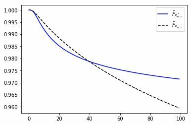
Example 3.12.

Let $X_{1},X_{2},X_{3}$ and $X^{*}_{1},X^{*}_{2},X^{*}_{3}$ be two sets of non-negative independent random variables such that $X_{i}\sim EG_{2}(5,\phi_{i},2),$ and $X^{*}_{i}\sim EG_{2}(5,\phi_{i}^{*},2)$,
$i=1,2,3.$ Let us choose $\phi_{1}=0.1,\phi_{2}=1.14,\phi_{3}=0.3$ and $\phi^{*}_{1}=0.6,\phi^{*}_{2}=0.9,\phi^{*}_{3}=0.04.$ It is clear that $(\phi_{1},\cdotp\cdotp\cdotp\cdotp\cdotp\phi_{n})\succeq^{m}(\phi^{*}_{1},\cdotp\cdotp\cdotp\cdotp\cdotp\phi^{*}_{n}).$ Now, from the Figure 1, in the next page, we observe that the reliability functions cross each other. This implies that $X_{n:n}\ngeq_{st}X^{*}_{n:n}.$

(a)

Figure 1: Presents plot of $\bar{F}_{X^{*}_{n:n}}$ and $\bar{F}_{X_{n:n}}.$

Disclosure statement

There is no potential conflict of interest. Both the authors have equally contributed towards the paper.

References

- [1] Okorie IE, Akpanta AC, Ohakwe J. The Exponentiated Gumbel Type-2 Distribution: Properties and Application: Hindawi Publishing Corporation, International Journal of Mathematics and Mathematical Sciences Volume 2016, Article ID 5898356.
- [2] Shaked M, Shanthikumar JG. Stochastic orders. New York: Springer; 2007.
- [3] Balakrishnan N, Haidari A, Masoumifard A. Stochastic Comparisons of Series and Parallel Systems With Generalized Exponential Components: IEEE Transactions on Reliability, Vol. 64, No. 1(333-348), March, 2015.
- [4] Fang L, Balakrishnan N. Ordering results for the smallest and largest order statistics from independent heterogeneous exponential–Weibull random variable: Statistics, 50:6, 1195-1205, DOI: 10.1080/02331888.2016.1142545.
- [5] Bashkar E, Torabi H, Roozegar R. Stochastic Comparisions Of Extreme Order Statistics in the Heterogeneous Exponentiated Scale Model: Journal of Theoretical and Applied Statistics, Vol. 16, No. 2 (June 2017)219-238.
- [6] Gupta N, Patra LK, Kumar S. Stochastic comparisons in systems with Frèchet distributed components Operations Research Letters(2015), DOI: 10.1016/j.orl.2015.09.009
- [7] Misra N, Misra AK. New results on stochastic comparisons of two-component series and parallel systems: Statist. Probab. Lett., vol. 82, pp. 283–290, 2012.
- [8] Torrado N, Kochar SC. Stochastic order relations among parallel systems from Weibull distributions: J Appl Probab. 2015;51:102–116.
- [9] Fang L, Zhang X. New results on stochastic comparison of order statistics from heterogeneous Weibull populations: J Korean Statist Soc. 2012;41:13–16.
- [10] Kundu A, Chowdhury S. Ordering properties of order statistics from heterogeneous exponentiated Weibull models: Statistics and Probability Letters 114 (2016) 119–127.
- [11] Nadarajah S, Kotz S. The exponentiated type distributions: Acta Applicandae Mathematica, vol. 92, no. 2, pp. 97–111, 2006.
- [12] Marshall AW, Olkin I, Arnold BC. Inequalities: theory of majorization and its applications, New York: Springer; 2011.