Effective Estimation of Deep Generative Language Models

Abstract

Advances in variational inference enable parameterisation of probabilistic models by deep neural networks. This combines the statistical transparency of the probabilistic modelling framework with the representational power of deep learning. Yet, due to a problem known as posterior collapse, it is difficult to estimate such models in the context of language modelling effectively. We concentrate on one such model, the variational auto-encoder, which we argue is an important building block in hierarchical probabilistic models of language. This paper contributes a sober view of the problem, a survey of techniques to address it, novel techniques, and extensions to the model. To establish a ranking of techniques, we perform a systematic comparison using Bayesian optimisation and find that many techniques perform reasonably similar, given enough resources. Still, a favourite can be named based on convenience. We also make several empirical observations and recommendations of best practices that should help researchers interested in this exciting field.

1 Introduction

Deep generative models (DGMs) are probabilistic latent variable models parameterised by neural networks (NNs). Specifically, DGMs optimised with amortised variational inference and reparameterised gradient estimates (Kingma and Welling, 2014; Rezende et al., 2014), better known as variational auto-encoders (VAEs), have spurred much interest in various domains, including computer vision and natural language processing (NLP).

In NLP, VAEs have been developed for word representation (Rios et al., 2018), morphological analysis (Zhou and Neubig, 2017), syntactic and semantic parsing (Corro and Titov, 2018; Lyu and Titov, 2018), document modelling (Miao et al., 2016), summarisation (Miao and Blunsom, 2016), machine translation (Zhang et al., 2016; Schulz et al., 2018; Eikema and Aziz, 2019), language and vision (Pu et al., 2016; Wang et al., 2017), dialogue modelling (Wen et al., 2017; Serban et al., 2017), speech modelling (Fraccaro et al., 2016), and, of course, language modelling (Bowman et al., 2016; Goyal et al., 2017). One problem remains common to the majority of these models, VAEs often learn to ignore the latent variables.

We investigate this problem, dubbed posterior collapse, in the context of language models (LMs). In a deep generative LM (Bowman et al., 2016), sentences are generated conditioned on samples from a continuous latent space, an idea with various practical applications. For example, one can constrain this latent space to promote generalisations that are in line with linguistic knowledge and intuition (Xu and Durrett, 2018). This also allows for greater flexibility in how the model is used, for example, to generate sentences that live—in latent space—in a neighbourhood of a given observation (Bowman et al., 2016). Despite this potential, VAEs that employ strong generators (e.g. recurrent NNs) tend to ignore the latent variable. Figure 1 illustrates this point: neighbourhood in latent space does not correlate to patterns in data space, and the model behaves just like a standard LM.

Recently, many techniques have been proposed to address this problem (§3 and §7) and they range from modifications to the objective to changes to the actual model. Some of these techniques have only been tested under different conditions and under different evaluation criteria, and some of them have only been tested outside NLP. This paper contributes: (1) a novel strategy based on constrained optimisation towards a pre-specified upper-bound on mutual information; (2) multimodal priors that by design promote increased mutual information between data and latent code; last and, arguably most importantly, (3) a systematic comparison—in terms of resources dedicated to hyperparameter search and sensitivity to initial conditions—of strategies to counter posterior collapse, including some never tested for language models (e.g. InfoVAE, LagVAE, soft free-bits, and multimodal priors).

Decoding	Generated sentence
Greedy	The company said it expects to report net income of $UNK-NUM million
Sample	They are getting out of my own things ?
	IBM also said it will expect to take next year .

(a) Greedy generation from prior samples (top) yields the same sentence every time, showing that the latent code is ignored. Yet, ancestral sampling (bottom) produces good sentences, showing that the recurrent decoder learns about the structure of English sentences.

The two sides hadn’t met since Oct. 18.

I don’t know how much money will be involved.

The specific reason for gold is too painful.

The New Jersey Stock Exchange Composite Index gained 1 to 16.

And some of these concerns aren’t known.

Prices of high-yield corporate securities ended unchanged.

(b) Homotopy: ancestral samples mapped from points along a linear interpolation of two given sentences as represented in latent space. The sentences do not seem to exhibit any coherent relation, showing that the model does not exploit neighbourhood in latent space to capture regularities in data space.

Figure 1: Sentences generated from Bowman et al. (2016)’s VAE trained without special treatment.

2 Density Estimation for Text

Density estimation for written text has a long history (Jelinek, 1980; Goodman, 2001), but in this work we concentrate on neural network models (Bengio et al., 2003), in particular, autoregressive ones (Mikolov et al., 2010). Following common practice, we model sentences independently, each a sequence $x=\langle x_{1},\ldots,x_{n}\rangle$ of $n=\absolutevalue{x}$ tokens.

2.1 Language models

A language model (LM) prescribes the generation of a sentence as a sequence of categorical draws parameterised in context, i.e. $P(x|\theta)=$

$$\prod_{i=1}^{\absolutevalue{x}}P(x_{i}|x_{<i},\theta)=\prod_{i=1}^{\absolutevalue{x}}\operatorname*{Cat}(x_{i}|f(x_{<i};\theta))~{}.$$ (1)

To condition on all of the available context, a fixed NN $f(\cdot)$ maps from a prefix sequence (denoted $x_{<i}$) to the parameters of a categorical distribution over the vocabulary. We estimate the parameters $\theta$ of the model by searching for a local optimum of the log-likelihood function $\mathcal{L}(\theta)\!=\!\mathbb{E}_{X}[\log P(x|\theta)]$ via stochastic gradient-based optimisation (Robbins and Monro, 1951; Bottou and Cun, 2004), where the expectation is taken w.r.t. the true data distribution and approximated with samples $x\sim\mathcal{D}$ from a data set of i.i.d. observations. Throughout, we refer to this model as RnnLM alluding to a particular choice of $f(\cdot;\phi)$ that employs a recurrent neural network (Mikolov et al., 2010).

2.2 Deep generative language models

Bowman et al. (2016) model observations as draws from the marginal of a DGM. An NN maps from a latent sentence embedding $z\in\mathbb{R}^{\operatorname*{\textit{d}}_{z}}$ to a distribution $P(x|z,\theta)$ over sentences,

$$P(x|\theta)=\int p(z)P(x|z,\theta)\differential z$$ (2)

$$=\int\!\mathcal{N}(z|0,I)\prod_{i=1}^{\absolutevalue{x}}\operatorname*{Cat}(x_{i}|f(z,x_{<i};\theta))\differential z~{},$$

where $z$ follows a standard Gaussian prior. Generation still happens one word at a time without Markov assumptions, but $f(\cdot)$ now conditions on $z$ in addition to the observed prefix. The conditional $P(x|z,\theta)$ is commonly referred to as generator or decoder. The quantity $P(x|\theta)$ is the marginal likelihood, essential for parameter estimation.

This model is trained to assign a high (marginal) probability to observations, much like standard LMs. Unlike standard LMs, it employs a latent space which can accommodate a low-dimensional manifold where discrete sentences are mapped to, via posterior inference $p(z|x,\theta)$, and from, via generation $P(x|z,\theta)$. This gives the model an explicit mechanism to exploit neighbourhood and smoothness in latent space to capture regularities in data space. For example, it may group sentences according to latent factors (e.g. lexical choices, syntactic complexity, etc.). It also gives users a mechanism to steer generation towards a specific purpose. For example, one may be interested in generating sentences that are mapped from the neighbourhood of another in latent space. To the extent this embedding space captures appreciable regularities, interest in this property is heightened.

Approximate inference

Marginal inference for this model is intractable and calls for variational inference (VI; Jordan et al., 1999), whereby an auxiliary and independently parameterised model $q(z|x,\lambda)$ approximates the true posterior $p(z|x,\theta)$. When this inference model is itself parameterised by a neural network, we have a case of amortised inference (Kingma and Welling, 2014; Rezende et al., 2014) and an instance of what is known as a VAE. Bowman et al. (2016) approach posterior inference with a Gaussian model

$$Z|\lambda,x \sim\mathcal{N}(\mathbf{u},\operatorname*{diag}(\mathbf{s}\odot\mathbf{s}))$$ (3)

$$[\mathbf{u},\mathbf{s}] =g(x;\lambda)$$

whose parameters, i.e. a location vector $\mathbf{u}\in\mathbb{R}^{D}$ and a scale vector $\mathbf{s}\in\mathbb{R}^{D}_{>0}$, are predicted by a neural network architecture $g(\cdot;\lambda)$ from an encoding of the complete observation $x$. In this work, we use a bidirectional recurrent encoder. Throughout the text we will refer to this model as SenVAE.

Parameter estimation

We can jointly estimate the parameters of both models (i.e. generative and inference) by locally maximising a lower-bound on the log-likelihood function (ELBO)

$$\mathcal{E}(\theta,\lambda)=\mathbb{E}_{X}\big{[}\mathbb{E}_{q(z|x,\lambda)}\left[\log P(x|z,\theta)\right]$$ (4)

$$-\operatorname*{KL}(q(z|x,\lambda)||p(z))\big{]}~{}.$$

For as long as we can reparameterise samples from $q(z|x,\lambda)$ using a fixed random source, automatic differentiation (Baydin et al., 2018) can be used to obtain unbiased gradient estimates of the ELBO (Kingma and Welling, 2014; Rezende et al., 2014).

3 Posterior Collapse

In VI, we make inferences using an approximation $q(z|x,\lambda)$ to the true posterior $p(z|x,\theta)$ and choose $\lambda$ as to minimise the KL divergence $\mathbb{E}_{X}[\operatorname*{KL}(q(z|x,\lambda)||p(z|x,\theta))]$. The same principle yields a lower-bound on log-likelihood used to estimate $\theta$ jointly with $\lambda$, thus making the true posterior $p(z|x,\theta)$ a moving target. If the estimated conditional $P(x|z,\theta)$ can be made independent of $z$, which in our case means relying exclusively on $x_{<i}$ to predict the distribution of $X_{i}$, the true posterior will be independent of the data and equal to the prior. Based on such observation, Chen et al. (2017) argue that information that can be modelled by the generator without using latent variables will be modelled that way—precisely because when no information is encoded in the latent variable the true posterior equals the prior and it is then trivial to reduce $\mathbb{E}_{X}[\operatorname*{KL}(q(z|x,\lambda)||p(z|x,\theta))]$ to $0$. This is typically diagnosed by noting that after training $\mathbb{\operatorname*{KL}}(q(z|x,\lambda)||p(z))\!\to\!0$ for most $x$: we say that the true posterior collapses to the prior. Alemi et al. (2018) show that the rate, $R=\mathbb{E}_{X}[\operatorname*{KL}(q(z|x,\lambda)||p(z))]$, is an upperbound to $I(X;Z|\lambda)$, the mutual information (MI) between $X$ and $Z$. Thus, if $\operatorname*{KL}(q(z|x,\lambda)||p(z))$ is close to zero for most training instances, MI is either $0$ or negligible. They also show that the distortion, $D=-\mathbb{E}_{X}[\mathbb{E}_{q(z|x,\lambda)}[\log P(x|z,\theta)]]$, relates to a lower-bound on MI (the lower-bound being $H-D$, where $H$ is the unknown data entropy).

A generator that makes no Markov assumptions, such as a recurrent LM, can potentially achieve $X_{i}\perp Z\mid x_{<i},\theta$, and indeed many have noticed that VAEs whose observation models are parameterised by such strong generators (or strong decoders) tend to ignore the latent representation (Bowman et al., 2016; Higgins et al., 2017; Sønderby et al., 2016; Zhao et al., 2018b). For this reason, a strategy to prevent posterior collapse is to weaken the decoder (Yang et al., 2017; Semeniuta et al., 2017; Park et al., 2018). In this work, we are interested in employing strong generators, thus we do not investigate weaker decoders. Other strategies involve changes to the optimisation procedure and manipulations to the objective that target local optima of the ELBO with non-negligible MI.

Annealing

Bowman et al. (2016) propose “KL annealing”, whereby the $\operatorname*{KL}$ term in the $\operatorname*{ELBO}$ is incorporated into the objective in gradual steps. This way the optimiser can focus on reducing distortion early on in training, potentially by increasing MI. They also propose to drop words from $x_{<i}$ at random to weaken the decoder—intuitively the model would have to rely on $z$ to compensate for missing history. We experiment with a slight modification of word dropout whereby we slowly vary the dropout rate from $1\to 0$. In a sense, we “anneal” from a weak to a strong generator.

Targeting rates

Another idea is to target a pre-specified rate (Alemi et al., 2018). Kingma et al. (2016) replace the $\operatorname*{KL}$ term in the ELBO with $\max(r,\operatorname*{KL}(q(z|x,\lambda)||p(z)))$, dubbed free bits (FB) because it allows encoding the first $r$ nats of information “for free”. As long as $\operatorname*{KL}(q(z|x,\lambda)||p(z))<r$, this does not optimise a proper ELBO (it misses the $\operatorname*{KL}$ term), and the $\max$ introduces a discontinuity. Chen et al. (2017) propose soft free bits (SFB), that instead multiplies the $\operatorname*{KL}$ term in the ELBO with a weighing factor $0<\beta\leq 1$ that is dynamically adjusted based on the target rate $r$: $\beta$ is incremented (or reduced) by $\omega$ if $R>\gamma r$ (or $R<\varepsilon r$). Note that this technique requires hyperparameters (i.e. $\gamma,\varepsilon,\omega$) besides $r$ to be tuned in order to determine how $\beta$ is updated.

Change of objective

We may also seek alternatives to the $\operatorname*{ELBO}$ as an objective and relate them to quantities of interest such as MI. A simple adaptation of the ELBO weighs its KL-term by a constant factor ($\beta$-VAE; Higgins et al., 2017). Setting $\beta<1$ promotes increased MI. Whilst being a useful counter to posterior collapse, low $\beta$ might lead to variational posteriors becoming point estimates. InfoVAE (Zhao et al., 2018b) mitigates this with a term aimed at minimising the divergence from the aggregated posterior $q(z|\lambda)=\mathbb{E}_{X}[q(z|x,\lambda)]$ to the prior. Following Zhao et al. (2018b), we approximate this with an estimate of maximum mean discrepancy (MMD; Gretton et al., 2012) in our experiments. Lagrangian VAE (LagVAE; Zhao et al., 2018a) casts VAE optimisation as a dual problem; it targets either maximisation or minimisation of (bounds on) $I(X;Z|\lambda)$ under constraints on the InfoVAE objective. In MI-maximisation mode, LagVAE maximises a weighted lower-bound on MI, $-\alpha D$, under two constraints, a maximum -ELBO and a maximum MMD, that prevent $p(z|x,\theta)$ from degenerating to a point mass. Reasonable values for these constraints have to be found empirically.

4 Minimum Desired Rate

We propose minimum desired rate (MDR), a technique to attain ELBO values at a pre-specified rate $r$ that does not suffer from the gradient discontinuities of FB, and does not introduce the additional hyperparameters of SFB. The idea is to optimise the ELBO subject to a minimum rate constraint $r$:

$$\max_{\theta,\lambda}~{}\mathcal{E}(\theta,\lambda),$$ (5)

$$~{}\text{s.t. }\mathbb{E}_{X}\left[\operatorname*{KL}(q(z|x,\lambda)||p(z))\right]>r~{}.$$

Because constrained optimisation is generally intractable, we optimise the Lagrangian (Boyd and Vandenberghe, 2004) $\Phi(\theta,\lambda,u)=$

$$\mathcal{E}(\theta,\lambda)-u(r-\mathbb{E}_{X}[\operatorname*{KL}(q(z|x,\lambda)||p(z))])$$ (6)

where $u\in\mathbb{R}_{\geq 0}$ is a positive Lagrangian multiplier. We define the dual function $\phi(u)=\max_{\theta,\lambda}~{}\Phi(\theta,\lambda,u)$ and solve the dual problem $\min_{u\in\mathbb{R}_{\geq 0}}~{}\phi(u)$. Local minima of the resulting min-max objective can be found by performing stochastic gradient descent with respect to $u$ and stochastic gradient ascent with respect to $\theta,\lambda$.

4.1 Relation to other techniques

It is insightful to compare MDR to the various techniques we surveyed in terms of the gradients involved in their optimisation. The losses minimised by $\operatorname*{KL}$ annealing, $\beta$-VAE, and SFB have the form $\ell_{\beta}(\theta,\lambda)=D+\beta R$, where $\beta\geq 0$. FB minimises the loss $\ell_{\text{FB}}(\theta,\lambda)=D+\max(r,R)$, where $r>0$ is the target rate. Last, with respect to $\theta$ and $\lambda$, MDR minimises the loss $\ell_{\text{MDR}}(\theta,\lambda)=D+R+u(r-R)$, where $u\in\mathbb{R}_{\geq 0}$ is the Lagrangian multiplier. And with respect to $u$, MDR minimises $\phi(u)=-D-R-u(R-r)$.

Let us inspect gradients with respect to the parameters of the VAE, namely, $$\theta \lambda \gradient_{\theta,\lambda}\ell_{\text{FB}}(\theta,\lambda)=$$ and . FB’s gradient

$$\gradient_{\theta,\lambda}D+\begin{cases}0&\text{if }R\leq r\\ \gradient_{\theta,\lambda}R&\text{otherwise}\end{cases}$$ (7a)

is discontinuous, that is, there is a sudden ‘jump’ from zero to a (possibly) large gradient w.r.t. $$R r \beta$$ when the rate dips above . KL annealing, -VAE, and SFB do not present such discontinuity

$$\gradient_{\theta,\lambda}\ell_{\beta}(\theta,\lambda)=\gradient_{\theta,\lambda}D+\beta\gradient_{\theta,\lambda}R~{},$$ (7b)

for $$\beta R$$ scales the gradient w.r.t. . The gradient of the MDR objective is

$$\gradient_{\theta,\lambda}\ell_{\text{MDR}}(\theta,\lambda)=\gradient_{\theta,\lambda}D+(1-u)\gradient_{\theta,\lambda}R$$ (7c)

which can be thought of as $$\gradient_{\theta,\lambda}\ell_{\beta}(\theta,\lambda) \beta 1-u$$ with dynamically set to at every gradient step.

Hence, MDR is another form of KL weighing, albeit one that targets a specific rate. Compared to $$\beta \beta \operatorname*{KL} \beta \beta \beta$$-VAE, MDR has the advantage that is not fixed but estimated to meet the requirements on rate. Compared to -annealing, MDR dispenses with a fixed schedule for updating , not only annealing schedules are fixed, they require multiple decisions (e.g. number of steps, linear or exponential increments) whose impact on the objective are not directly obvious. Most similar then, seems SFB. Like MDR, it flexibly updates by targeting a rate. However, differences between the two techniques become apparent when we observe how is updated. In case of SFB:

$$\beta^{(t+1)}=\beta^{(t)}+\begin{cases}\omega&\text{if }R>\gamma r\\ -\omega&\text{if }R<\varepsilon r\end{cases}$$ (8a)

where $$\omega \gamma \varepsilon$$, and are hyperparameters. In case of MDR (not taking optimiser-specific dynamics into account):

$$u^{(t+1)}=u^{(t)}-\rho\partialderivative{\phi(u)}{u}=u^{(t)}+\rho(R-r)$$ (8b)

where $$\rho$$ is a learning rate. From this, we conclude that MDR is akin to SFB, but MDR’s update rule is a direct consequence of Lagrangian relaxation and thus dispenses with the additional hyperparameters in SFB’s handcrafted update rule.

5 Expressive Priors

Suppose we employ a multimodal prior $p(z|\theta)$, e.g. a mixture of Gaussians, and suppose we employ a unimodal posterior approximation, e.g. the typical diagonal Gaussian. This creates a mismatch between the prior and the posterior approximation families that makes it impossible for $\operatorname*{KL}(q(z|x,\lambda)||p(z|\theta))$ to be precisely $0$. For the aggregated posterior $q(z|\lambda)$ to match the prior, the inference model would have to—on average—cover all of the prior’s modes. Since the inference network is deterministic, it can only do so as a function of the conditioning input $x$, thus increasing $I(X;Z|\lambda)$. Admittedly, this conditioning might still only capture shallow features of $x$, and the generator may still choose to ignore the latent code, keeping $I(X;Z|\theta)$ low, but the potential seems to justify an attempt. This view builds upon Alemi et al. (2018)’s information-theoretic view which suggests that the prior regularises the inference model capping $I(X;Z|\lambda)$. Thus, we modify SenVAE to employ a more complex, ideally multimodal, parametric prior $p(z|\theta)$ and fit its parameters.

MoG

Our first option is a uniform mixture of Gaussians (MoG), i.e. $p(z|\theta)=$

$$\frac{1}{C}\sum_{c=1}^{C}\mathcal{N}(z|\boldsymbol{\mu}^{(c)},\operatorname*{diag}(\boldsymbol{\sigma}^{(c)}\odot\boldsymbol{\sigma}^{(c)}))$$ (9)

where the Gaussian parameters are optimised along with other generative parameters. Note that though we give this prior up to $C$ modes, the optimiser might merge some of them (by learning approximately the same location and scale).

VampPrior

Motivated by the fact that, for a fixed posterior approximation, the prior that optimises the $\operatorname*{ELBO}$ equals $\mathbb{E}_{X}[q(z|x,\lambda)]$, Tomczak and Welling (2018) propose the VampPrior, a variational mixture of posteriors:

$$p(z|\theta)=\frac{1}{C}\sum_{c=1}^{C}q(z|v^{(c)},\lambda)$$ (10)

where $v^{(c)}$ is a learned pseudo input—in their case a continuous vector. Again the parameters of the prior, i.e. $\{v^{(c)}\}_{c=1}^{C}$, are optimised in the ELBO. In our case, the input to the inference network is a discrete sentence, which is incompatible with the design of the VampPrior. Thus, we propose to bypass the inference network’s embedding layer and estimate a sequence of word embeddings, which makes up a pseudo input. That is, $v^{(c)}$ is a sequence $\langle\mathbf{v}^{(c)}_{1},\ldots,\mathbf{v}^{(c)}_{l_{c}}\rangle$ where $\mathbf{v}^{(c)}_{i}$ has the dimensionality of our embeddings, and $l_{c}$ is the length of the sequence (fixed at the beginning of training). Note, however, that for this prior to be multimodal, the inference model must already encode information in $Z$, thus there is some gambling in its design.

6 Experiments

Our goal is to identify which techniques are effective in training VAEs for language modelling. Our evaluation concentrates on intrinsic metrics: negative log-likelihood (NLL), perplexity per token (PPL), rate ($R$), distortion ($D$), the number of active units (AU; Burda et al., 2015)) and gap in the accuracy of next word prediction (given gold prefixes) when decoding from a posterior sample versus decoding from a prior sample (Acc${}_{\text{gap}}$).

For VAE models, NLL (and thus PPL) can only be estimated. We use importance sampling (IS)

$$\!\!\!\!\!\!P(x|\theta)=\int p(z,x|\theta)\differential z\overset{\text{IS}}{=}\int q(z|x)\frac{p(z,x|\theta)}{q(z|x)}\differential z\\ \!\!\overset{\text{MC}}{\approx}\frac{1}{S}\sum_{s=1}^{S}\frac{p(z^{(s)},x|\theta)}{q(z^{(s)}|x)}~{}\text{ where }z^{(s)}\!\sim q(z|x)$$ (11)

with our trained approximate posterior as importance distribution (we use $S=1000$ samples).

We first report on experiments using the English Penn Treebank (PTB; Marcus et al., 1993).

RnnLM

The baseline RnnLM generator is a building block for all of our SenVAEs, thus we validate its performance as a strong standalone generator. We highlight that it outperforms an external baseline that employs a comparable number of parameters (Dyer et al., 2016) and that this performance boost is mostly due to tying embeddings with the output layer. Appendix A.1 presents the complete architecture and a comparison.

Bayesian optimisation

The techniques we compare are sensitive to one or more hyperparameters (see Table 1), which we tune using Bayesian optimisation (BO) towards minimising estimated NLL of the validation data. For each technique, we ran 25 iterations of BO, each iteration encompassing training a model to full convergence. This was sufficient for the hyperparameters of each technique to converge. See Appendix A.2 for details.

On optimisation strategies

Technique	Hyperparameters
KL annealing	increment $\gamma$ ($2\times 10^{-5}$)
Word dropout (WD)	decrement $\gamma$ ($2\times 10^{-5}$)
FB and MDR	target rate $r$ ($5$)
SFB	$r$ ($6.46$), $\gamma$ ($1.05$), $\varepsilon$ ($1$), $\omega$ ($0.01$)
$\beta$-VAE	KL weight $\beta$ ($0.66$)
InfoVAE	$\beta$ ($0.7$), $\lambda$ ($31.62$)
LagVAE	$\alpha$ ($-21.7$), target MMD ($0.0017$)
	target -ELBO ($100.8$)

Table 1: Techniques and their hyperparameters.

Mode		$D$	$R$		PPL$\downarrow$	AU$\uparrow$	Acc${}_{\text{gap}}$
RnnLM		-	-		107.1$\pm$0.5	-	-
Vanilla		118.4	0.0		105.7$\pm$0.4	0	0.0
Annealing		115.3	3.3		103.7$\pm$0.3	17	6.0
WD		117.6	0.0		102.5$\pm$0.6	0	0.0
FB		113.3	5.0		101.9$\pm$0.8	14	5.8
SFB		112.0	6.4		101.0$\pm$0.5	18	7.0
MDR		113.5	5.0		102.1$\pm$0.5	13	6.2
$\beta$-VAE		113.0	5.3		101.7$\pm$0.5	11	6.1
InfoVAE		113.5	4.3		100.8$\pm$0.4	10	5.2
LagVAE		112.1	6.5		101.6$\pm$0.7	24	6.9

Table 2: Performance (avg$\pm\text{std}$ across $5$ independent runs) of SenVAE on the PTB validation set. Standard deviations for $D$ and $R$ are at most $0.2$.

First, we assess the effectiveness of techniques that aim at promoting local optima of SenVAE with better MI tradeoff. As for the architecture, the approximate posterior $q(z|x,\lambda)$ employs a bidirectional recurrent encoder, and the generator $P(x|z,\theta)$ is essentially our RnnLM initialised with a learned projection of $z$ (complete specification in A.1). We train with Adam (Kingma and Ba, 2014) with default parameters and a learning rate of $10^{-3}$ until convergence five times for each technique.

Results can be found in Table 2. First, note how the vanilla VAE (no special treatment) encodes no information in latent space ($R=0$). Then note that all techniques converged to VAEs that attain better PPL than the RnnLM and vanilla VAE, and all but annealed word dropout did so at non-negligible rate. Notably, the two most popular techniques, word dropout and $\operatorname*{KL}$ annealing, perform sub-par to the other techniques. The techniques that work well at non-negligible rates can be separated into two groups: one based on a change of objective (i.e., $\beta$-VAE, InfoVAE and LagVAE), another based on targeting a specific rate (i.e., FB, SFB, and MDR). InfoVAE, LagVAE and SFB all require tuning of multiple hyperparameters. InfoVAE and LagVAE, in particular, showed poor performance without this careful tuning. In the first group, consider LagVAE, for example. Though Zhao et al. (2018a) argue that the magnitude of $\alpha$ is not particularly important (in MI-maximisation mode, they fixed it to $-1$), we could not learn a useful SenVAE with LagVAE until we allowed BO to also estimate the magnitude of $\alpha$. Once BO converges to the values in Table 1, the method does perform quite well.

Generally, it is hard to believe that hyperparameters transfer across data sets, thus it is fair to expect that this exercise will have to be repeated every time. We argue that the rate hyperparameter common to the techniques in the second group is more interpretable and practical in most cases. For example, it is easy to grid-search against a handful of values. Hence, we further investigate FB and MDR by varying the target rate further (from $5$ to $50$). SFB is left out, for MDR generalises SFB’s handcrafted update rule. We observe that FB and MDR attain essentially the same PPL across rates, though MDR attains the desired rate earlier on in training, especially for higher targets (where FB fails at reaching the specified rate). Importantly, at the end of training, the validation rate is closer to the target for MDR. Appendix B supports these claims. Though Acc${}_{\text{gap}}$ already suggests it, Figure 2 shows more visibly that MDR leads to output Categorical distributions that are more sensitive to the latent encoding. We measure this sensitivity in terms of symmetrised KL between output distributions obtained from a posterior sample and output distributions obtained from a prior sample for the same time step given an observed prefix.

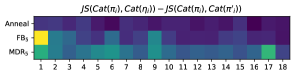
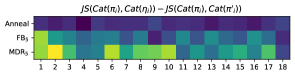
Figure 2: Sensitivity of output distributions to posterior samples measured in terms of symmetrised KL (JS). We obtain $51$ (top) validation and $84$ (bottom) test instances of length $20$ and report on their output distributions per time step. To account for expected variability, we report $\operatorname*{JS}(\operatorname*{Cat}(\pi_{i})||\operatorname*{Cat}(\eta_{i}))-\operatorname*{JS}(\operatorname*{Cat}(\pi_{i})||\operatorname*{Cat}(\pi^{\prime}_{i}))$, where $\eta_{i}$ conditions on a prior sample, and $\pi_{i}$ and $\pi^{\prime}_{i}$ condition on different posterior samples, averaged over $10$ experiments.

On expressive priors

Model		$D$	$R$	PPL$\downarrow$	AU$\uparrow$	Acc${}_{\text{gap}}$
RnnLM		-	-	84.5$\pm$ 0.5	-	-
$\mathcal{N}$/$\mathcal{N}$		103.5	5.0	81.5$\pm$ 0.5	13	5.4
MoG/$\mathcal{N}$		103.3	5.0	81.4$\pm$ 0.5	32	5.8
Vamp/$\mathcal{N}$		103.1	5.0	81.2$\pm$ 0.4	22	5.8

Table 3: Performance on the PTB test set for different priors ($\mathcal{N}$, MoG, Vamp). Standard deviations of $D$, $R$, and Acc${}_{\text{gap}}$ are at most $0.1$.

Second, we compare the impact of expressive priors. This time, prior hyperparameters were selected via grid search and can be found in Appendix A.1. All models are trained with a target rate of $5$ using MDR, with settings otherwise the same as the previous experiment. In Table 3 it can be seen that more expressive priors do not improve perplexity further, though they seem to encode more information in the latent variable—note the increased number of active units and the increased gap in accuracy. One may wonder whether stronger priors allow us to target higher rates without hurting PPL. This does not seem to be the case: as we increase rate to $50$, all models perform roughly the same, and beyond $20$ performance degrades quickly. The models did, however, show a further increase in active units (VampPrior) and accuracy gap (both priors). Again, Appendix B contains plots supporting these claims.

	Yahoo					Yelp
Model	$R$	NLL$\downarrow$	PPL$\downarrow$	AU$\uparrow$		$R$	NLL$\downarrow$	PPL$\downarrow$	AU$\uparrow$
RnnLM	-	$328.0$$\pm 0.3$	-	-		-	$358.1$$\pm 0.6$	-	-
Lagging	$5.7$$\pm 0.7$	$326.7$$\pm 0.1$	-	$15.0$$\pm 3.5$		$3.8$$\pm 0.2$	$355.9$$\pm 0.1$	-	$11.3$$\pm 1.0$
$\beta$-VAE ($\beta=0.4$)	$6.3$$\pm 1.7$	$328.7$$\pm 0.1$	-	$8.0$$\pm 5.2$		$4.2$$\pm 0.4$	$358.2$$\pm 0.3$	-	$4.2$$\pm 3.8$
Annealing	$0.0$$\pm 0.0$	$328.6$$\pm 0.0$	-	$0.0$$\pm 0.0$		$0.0$$\pm 0.0$	$357.9$$\pm 0.1$	-	$0.0$$\pm 0.0$
Vanilla	$0.0$$\pm 0.0$	$328.9$$\pm 0.1$	$61.4$$\pm 0.1$	$0.0$$\pm 0.0$		$0.0$$\pm 0.0$	$358.3$$\pm 0.2$	$40.8$$\pm 0.1$	$0.0$$\pm 0.0$
$\mathcal{N}$/$\mathcal{N}$	$5.0$$\pm 0.0$	$328.1$$\pm 0.1$	$60.8$$\pm 0.1$	$4.0$$\pm 0.7$		$5.0$$\pm 0.0$	$357.5$$\pm 0.2$	$40.4$$\pm 0.1$	$4.2$$\pm 0.4$
MoG/$\mathcal{N}$	$5.0$$\pm 0.1$	$327.5$$\pm 0.2$	$60.5$$\pm 0.1$	$5.0$$\pm 0.7$		$5.0$$\pm 0.0$	$359.5$$\pm 0.5$	$41.2$$\pm 0.3$	$2.2$$\pm 0.4$

Table 4: Performance on the Yahoo/Yelp corpora. Top rows taken from (He et al., 2019)

Generated samples

Sample	Closest training instance	TER
For example, the Dow Jones Industrial Average fell almost 80 points to close at 2643.65.	By futures-related program buying, the Dow Jones Industrial Average gained 4.92 points to close at 2643.65.	$0.38$
The department store concern said it expects to report profit from continuing operations in 1990.	Rolls-Royce Motor Cars Inc. said it expects its U.S. sales to remain steady at about 1,200 cars in 1990.	$0.59$
The new U.S. auto makers say the accord would require banks to focus on their core businesses of their own account.	International Minerals said the sale will allow Mallinckrodt to focus its resources on its core businesses of medical products, specialty chemicals and flavors.	$0.78$

Figure 3: Samples from SenVAE (MoG prior) trained via MDR: we sample from the prior and decode greedily. We also show the closest training instance in terms of a string edit distance (TER).

The inquiry soon focused on the judge.

The judge declined to comment on the floor.

The judge was dismissed as part of the settlement.

The judge was sentenced to death in prison.

The announcement was filed against the SEC.

The offer was misstated in late September.

The offer was filed against bankruptcy court in New York.

The letter was dated Oct. 6.

Figure 4: Latent space homotopy from a properly trained SenVAE. Note the smooth transition of topic and grammatically of the samples.

Figure 3 shows samples from a well-trained SenVAE, where we decode greedily from a prior sample—this way, all variability is due to the generator’s reliance on the latent sample. Recall that a vanilla VAE ignores $z$ and thus greedy generation from a prior sample is essentially deterministic in that case (see Figure 1(a)). Next to the samples we show the closest training instance, which we measure in terms of an edit distance (TER; Snover et al., 2006). This “nearest neighbour” helps us assess whether the generator is producing novel text or simply reproducing something it memorised from training. In Figure 4 we show a homotopy: here we decode greedily from points lying between a posterior sample conditioned on the first sentence and a posterior sample conditioned on the last sentence. In contrast to the vanilla VAE (Figure 1(b)), neighbourhood in latent space is now used to capture some regularities in data space. These samples add support to the quantitative evidence that our DGMs have been trained not to neglect the latent space. In Appendix B we provide more samples.

Other datasets

To address the generalisability of our claims to other, larger, datasets, we report results on the Yahoo and Yelp corpora Yang et al. (2017) in Table 4. We compare to the work of He et al. (2019), who proposed to mitigate posterior collapse with aggressive training of the inference network, optimising the inference network multiple steps for each step of the generative network.. We report on models trained with the standard prior as well as an MoG prior both optimised with MDR, and a model trained without optimisation techniques. It can be seen that MDR compares favourably to other optimisation techniques reported in He et al. (2019). Whilst aggressive training of the inference network performs slightly better in terms of NLL and leads to more active units, it slows down training by a factor of 4. The MoG prior improves results on Yahoo but not on Yelp. This may indicate that a multimodal prior does offer useful extra capacity to the latent space, at the cost of more instability in optimisation. This confirms that targeting a pre-specified rate leads to VAEs that are not collapsed without hurting NLL.

Recommendations

We recommend targeting a specific rate via MDR instead of annealing (or word dropout). Besides being simple to implement, it is fast and straightforward to use: pick a rate by plotting validation performance against a handful of values. Stronger priors, on the other hand, while showing indicators of higher mutual information (e.g. AU and Acc${}_{\text{gap}}$), seem less effective than MDR. Use IS estimates of NLL, rather than single-sample ELBO estimates, for model selection, for the latter can be too loose of a bound and too heavily influenced by noisy estimates of KL. Use many samples for a tight bound. Inspect sentences greedily decoded from a prior (or posterior) sample as this shows whether the generator is at all sensitive to the latent code. Retrieve nearest neighbours to spot copying behaviour.

7 Related Work

In NLP, posterior collapse was probably first noticed by Bowman et al. (2016), who addressed it via word dropout and KL scaling. Further investigation revealed that in the presence of strong generators, the ELBO itself becomes the culprit (Chen et al., 2017; Alemi et al., 2018), as it lacks a preference regarding MI. Posterior collapse has also been ascribed to approximate inference (Kim et al., 2018; Dieng and Paisley, 2019). Beyond the techniques compared and developed in this work, other solutions have been proposed, including modifications to the generator (Semeniuta et al., 2017; Yang et al., 2017; Park et al., 2018; Dieng et al., 2019), side losses based on weak generators (Zhao et al., 2017), factorised likelihoods (Ziegler and Rush, 2019; Ma et al., 2019), cyclical annealing (Liu et al., 2019) and changes to the ELBO (Tolstikhin et al., 2018; Goyal et al., 2017).

Exploiting a mismatch in correlation between the prior and the approximate posterior, and thus forcing a lower-bound on the rate, is the principle behind $\delta$-VAEs (Razavi et al., 2019) and hyperspherical VAEs (Xu and Durrett, 2018). The generative model of $\delta$-VAEs has one latent variable per step of the sequence, i.e. $z=\langle z_{1},\ldots,z_{|x|}\rangle$, making it quite different from that of the SenVAEs considered here. Their mean-field inference model is a product of independent Gaussians, one per step, but they construct a correlated Gaussian prior by making the prior distribution over the next step depend linearly on the previous step, i.e. $Z_{i}|z_{i-1}\sim\mathcal{N}(\alpha z_{i-1},\sigma)$ with hyperparameters $\alpha$ and $\sigma$. Hyperspherical VAEs work on the unit hypersphere with a uniform prior and a non-uniform VonMises-Fisher posterior approximation (Davidson et al., 2018). Note that, though in this paper we focused on Gaussian (and mixture of Gaussians, e.g. MoG and VampPrior) priors, MDR is applicable for whatever choice of prescribed prior. Whether its benefits stack with the effects due to different priors remains an empirical question.

GECO (Rezende and Viola, 2018) casts VAE optimisation as a dual problem, and in that it is closely related to our MDR and the LagVAE. GECO targets minimisation of $\mathbb{E}_{X}[\operatorname*{KL}(q(z|x,\lambda)||p(z))]$ under constraints on distortion, whereas LagVAE targets either maximisation or minimisation of (bounds on) $I(X;Z|\lambda)$ under constraints on the InfoVAE objective. Contrary to MDR, GECO focuses on latent space regularisation and offers no explicit mechanism to mitigate posterior collapse.

Recently Li et al. (2019) proposed to combine FB, KL scaling, and pre-training of the inference network’s encoder on an auto-encoding objective. Their techniques are complementary to ours in so far as their main finding—the mutual benefits of annealing, pre-training, and lower-bounding KL—is perfectly compatible with ours (MDR and multimodal priors).

8 Discussion

SenVAE is a deep generative model whose generative story is rather shallow, yet, due to its strong generator component, it is hard to make effective use of the extra knob it offers. In this paper, we have introduced and compared techniques for effective estimation of such a model. We show that many techniques in the literature perform reasonably similarly (i.e. FB, SFB, $\beta$-VAE, InfoVAE), though they may require a considerable hyperparameter search (e.g. SFB and InfoVAE). Amongst these, our proposed optimisation subject to a minimum rate constraint is simple enough to tune (as FB it only takes a pre-specified rate and unlike FB it does not suffer from gradient discontinuities), superior to annealing and word dropout, and require less resources than strategies based on multiple annealing schedules and/or aggressive optimisation of the inference model. Other ways to lower-bound rate, such as by imposing a multimodal prior, though promising, still require a minimum desired rate.

The typical RnnLM is built upon an exact factorisation of the joint distribution, thus a well-trained architecture is hard to improve upon in terms of log-likelihood of gold-standard data. Our interest in latent variable models stems from the desire to obtain generative stories that are less opaque than that of an RnnLM, for example, in that they may expose knobs that we can use to control generation and a hierarchy of steps that may award a degree of interpretability to the model. The SenVAE is not that model, but it is a crucial building block in the pursue for hierarchical probabilistic models of language. We hope this work, i.e. the organised review it contributes and the techniques it introduces, will pave the way to deeper—in statistical hierarchy—generative models of language.

Appendix A Architectures and Hyperparameters

In order to ensure that all our experiments are fully reproducible, this section provides an extensive overview of the model architectures, as well as model and optimisation hyperparameters.

Some hyperparameters are common to all experiments, e.g. optimiser and dropout, they can be found in Table 5. All models were optimised with Adam using default settings (Kingma and Ba, 2014). To regularise the models, we use dropout with a shared mask across time-steps (Zaremba et al., 2014) and weight decay proportional to the dropout rate (Gal and Ghahramani, 2015) on the input and output layers of the generative networks (i.e. RnnLM and the recurrent decoder in SenVAE). No dropout is applied to layers of the inference network as this does not lead to consistent empirical benefits and lacks a good theoretical basis. Gradient norms are clipped to prevent exploding gradients, and long sentences are truncated to three standard deviations above the average sentence length in the training data.

Parameter	Value
Optimizer	Adam
Optimizer Parameters	$\beta_{1}=0.9,\beta_{2}=0.999$
Learning Rate	0.001
Batch Size	64
Decoder Dropout Rate ($\rho$)	0.4
Weight Decay	$\frac{1-\rho}{|\mathcal{D}|}$
Maximum Sentence Length	59
Maximum Gradient Norm	1.5

Table 5: Experimental settings.

A.1 Architectures

Model	Parameter	Value
A	embedding units ($\operatorname*{\textit{d}}_{e}$)	256
A	vocabulary size ($\operatorname*{\textit{d}}_{v}$)	25643
R and S	decoder layers ($L^{\theta}$)	2
R and S	decoder hidden units ($\operatorname*{\textit{d}}_{h}^{\theta}$)	256
S	encoder hidden units ($\operatorname*{\textit{d}}_{h}^{\lambda}$)	256
S	encoder layers ($L^{\lambda}$)	1
S	latent units ($\operatorname*{\textit{d}}_{z}$)	32
MoG	mixture components ($C$)	100
VampPrior	pseudo inputs ($C$)	100

Table 6: Architecture parameters: all (A), RnnLM (R), SenVAE (S).

This section describes the components that parameterise our models. We use mnemonic blocks $\operatorname*{layer}(\text{inputs};\text{parameters})$ to describe architectures. Table 6 lists hyperparameters for the models discussed in what follows.

RnnLM

At each step, an RnnLM parameterises a categorical distribution over the vocabulary, i.e. $X_{i}|x_{<i}\sim\operatorname*{Cat}(f(x_{<i};\theta))$, where $f(x_{<i};\theta)=\operatorname*{softmax}(\mathbf{o}_{i})$ and

$$\mathbf{e}_{i} =\operatorname*{emb}(x_{i};\theta_{\text{emb}})$$ (12a)

$$\mathbf{h}_{i} =\operatorname*{GRU}(\mathbf{h}_{i-1},\mathbf{e}_{i-1};\theta_{\text{gru}})$$ (12b)

$$\mathbf{o}_{i} =\operatorname*{affine}(\mathbf{h}_{i};\theta_{\text{out}})~{}.$$ (12c)

We employ an embedding layer ($\operatorname*{emb}$), one (or more) $\operatorname*{GRU}$ cell(s) ($\mathbf{h}_{0}\in\theta$ is a parameter of the model), and an $\operatorname*{affine}$ layer to map from the dimensionality of the GRU to the vocabulary size. Table 7 compares our RnnLM to an external baseline with a comparable number of parameters.

Model	PPL$\downarrow$	PPL${}^{\text{Dyer}}\downarrow$
Dyer et al. (2016)	$93.5$	$113.4$
RnnLM	84.5$\pm$ 0.52	$102.1$

Table 7: Baseline LMs on the PTB test set: $\text{avg}\pm\text{std}$ over $5$ independent runs. Unlike us, Dyer et al. (2016) removed the end of sentence token for evaluation, thus the last column reports perplexity computed that way.

Gaussian SenVAE

A Gaussian SenVAE also parameterises a categorical distribution over the vocabulary for each given prefix, but, in addition, it conditions on a latent embedding $Z\sim\mathcal{N}(0,I)$, i.e. $X_{i}|z,x_{<i}\sim\operatorname*{Cat}(f(z,x_{<i};\theta))$ where $f(z,x_{<i};\theta)=\operatorname*{softmax}(\mathbf{o}_{i})$ and

$$\mathbf{e}_{i} =\operatorname*{emb}(x_{i};\theta_{\text{emb}})$$ (13a)

$$\mathbf{h}_{0} =\tanh(\operatorname*{affine}(z;\theta_{\text{init}}))$$ (13b)

$$\mathbf{h}_{i} =\operatorname*{GRU}(\mathbf{h}_{i-1},\mathbf{e}_{i-1};\theta_{\text{gru}})$$ (13c)

$$\mathbf{o}_{i} =\operatorname*{affine}(\mathbf{h}_{i};\theta_{\text{out}})~{}.$$ (13d)

Compared to RnnLM, we modify $f$ only slightly by initialising GRU cell(s) with $\mathbf{h}_{0}$ computed as a learnt transformation of $z$. Because the marginal of the Gaussian SenVAE is intractable, we train it via variational inference using an inference model $q(z|x,\lambda)=\mathcal{N}(z|\mathbf{u},\operatorname*{diag}(\mathbf{s}\odot\mathbf{s}))$ where

$$\mathbf{e}_{i} =\operatorname*{emb}(x_{i};\theta_{\text{emb}})$$ (14a)

$$\mathbf{h}_{1}^{n} =\operatorname*{BiGRU}(\mathbf{e}_{1}^{n},\mathbf{h}_{0};\lambda_{\text{enc}})$$ (14b)

$$\mathbf{u} =\operatorname*{affine}(\mathbf{h}_{n};\lambda_{\text{loc}})$$ (14c)

$$\mathbf{s} =\operatorname*{softplus}(\operatorname*{affine}(\mathbf{h}_{n};\lambda_{\text{scale}}))~{}.$$ (14d)

Note that we reuse the embedding layer from the generative model. Finally, a sample is obtained via $z=\mathbf{u}+\mathbf{s}\odot\epsilon$ where $\epsilon\sim\mathcal{N}(0,I_{\operatorname*{\textit{d}}_{z}})$.

MoG prior

We parameterise $C$ diagonal Gaussians, which are mixed uniformly. To do so we need $C$ location vectors, each in $\mathbb{R}^{\operatorname*{\textit{d}}_{z}}$, and $C$ scale vectors, each in $\mathbb{R}^{\operatorname*{\textit{d}}_{z}}_{>0}$. To ensure strict positivity for scales we make $\boldsymbol{\sigma}^{(c)}=\operatorname*{softplus}(\hat{\boldsymbol{\sigma}}^{(c)})$. The set of generative parameters $\theta$ is therefore extended with $\{\boldsymbol{\mu}^{(c)}\}_{c=1}^{C}$ and $\{\hat{\boldsymbol{\sigma}}^{(c)}\}_{c=1}^{C}$, each in $\mathbb{R}^{\operatorname*{\textit{d}}_{z}}$.

VampPrior

For this we estimate $C$ sequences $\{v^{(c)}\}_{c=1}^{C}$ of input vectors, each sequence $v^{(c)}=\langle\mathbf{v}_{1}^{(c)},\ldots,\mathbf{v}_{l_{k}}^{(c)}\rangle$ corresponds to a pseudo-input. This means we extend the set of generative parameters $\theta$ with $\{\mathbf{v}_{i}^{(c)}\}_{i=1}^{l_{c}}$, each in $\mathbb{R}^{\operatorname*{\textit{d}}_{e}}$, for $c=1,\ldots,C$. For each $c$, we sample $l_{c}$ at the beginning of training and keep it fixed. Specifically, we drew $C$ samples from a normal, $l_{c}\sim\mathcal{N}(\cdot|\mu_{l},\sigma_{l})$, which we rounded to the nearest integer. $\mu_{l}$ and $\sigma_{l}$ are the dataset sentence length mean and variance respectively.

A.2 Bayesian optimisation

Parameter	Value
Objective Function	Validation NLL
Kernel	Matern52
Acquisition Function	Expected Improvement
Parameter Inference	MCMC
MCMC Samples	10
Leapfrog Steps	20
Burn-in Samples	100

Table 8: Bayesian optimisation settings.

Bayesian optimisation (BO) is an efficient method to approximately search for global optima of a (typically expensive to compute) objective function $y=f(\mathbf{x})$, where $\mathbf{x}\in\operatorname{\mathbb{R}}^{M}$ is a vector containing the values of $M$ hyperparameters that may influence the outcome of the function (Snoek et al., 2012). Hence, it forms an alternative to grid search or random search (Bergstra and Bengio, 2012) for tuning the hyperparameters of a machine learning algorithm. BO works by assuming that our observations $y_{n}|\mathbf{x}_{n}$ (for $n=1,\ldots,N$) are drawn from a Gaussian process (GP; Rasmussen and Williams, 2005). Then based on the GP posterior, we can design and infer an acquisition function. This acquisition function can be used to determine where to “look next” in parameter-space, i.e. it can be used to draw $\mathbf{x}_{N+1}$ for which we then evaluate the objective function $f(x_{N+1})$. This procedure iterates until a set of optimal parameters is found with some level of confidence.

In practice, the efficiency of BO hinges on multiple choices, such as the specific form of the acquisition function, the covariance matrix (or kernel) of the GP and how the parameters of the acquisition function are estimated. Our objective function is the (importance-sampled) validation NLL, which can only be computed after a model convergences (via gradient-based optimisation of the ELBO). We follow the advice of Snoek et al. (2012) and use MCMC for estimating the parameters of the acquisition function. This reduced the amount of objective function evaluations, speeding up the overall search. Other settings were also based on results by Snoek et al. (2012), and we refer the interested reader to that paper for more information about BO in general. A summary of all relevant settings of BO can be found in Table 8. We used the GPyOpt library (authors, 2016) to implement this procedure.

Appendix B Additional Empirical Evidence

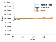
(a) Rate over time for $r=10$.

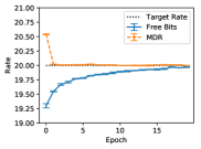
(b) Rate over time for $r=20$.

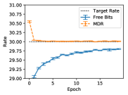
(c) Rate over time for $r=30$.

Figure 5: Rate progression on the training set in the first $20$ epochs of training for SenVAE trained with free bits (FB) or minimum desired rate (MDR). One can observe that at higher rates, FB struggles to achieve the target rate, whereas MDR achieves the target rate after a few epochs.

In Figure 5 we inspect how MDR and FB approach different target rates (namely, $10$, $20$, and $30$). Note how MDR does so more quickly, especially at higher rates. Figure 6(a) shows that in terms of validation perplexity, MDR and FB perform very similarly across target rates. However, Figure 6(b) shows that at the end of training the difference between the target rate and the validation rate is smaller for MDR.

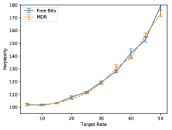
(a) PPL ($\downarrow$) for various target rates.

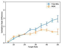
(b) Target rate minus validation rate at the end of training for various targets (lower means better).

Figure 6: Validation results for SenVAE trained with free bits (FB) or minimum desired rate (MDR).

Figure 7 compares variants of SenVAE trained with MDR for various rates: a Gaussian-posterior and Gaussian-prior (blue-solid) to a Gaussian-posterior and Vamp-prior (orange-dashed). They perform essentially the same in terms of perplexity (Figure 7(a)), but the variant with the stronger prior relies more on posterior samples for reconstruction (Figure 7(b)).

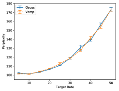
(a) Perplexity on validation set: models perform similarly well and perplexity degrades considerably for $r>20$.

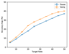
(b) Accuracy gap: VAEs with stronger latent components rely more on posterior samples for reconstruction.

Figure 7: Comparison of SenVAEs trained with standard prior and Gaussian posterior (Gauss) and Vamp prior and Gaussian posterior (Vamp) to attain pre-specified rates.

Finally, we list additional samples: Figure 8 lists samples from RnnLM, vanilla SenVAE and effectively trained variants (via MDR with target rate $r=10$); Figure 9 lists homotopies from SenVAE models.

Model	Sample	Closest training instance	TER
RnnLM	The Dow Jones Industrial Average jumped 26.23 points to 2662.91 on 2643.65.	The Dow Jones Industrial Average fell 26.23 points to 2662.91.	$0.23$
	The companies said they are investigating their own minds with several carriers, including the National Institutes of Health and Human Services Department of Health,,	The Health and Human Services Department currently forbids the National Institutes of Health from funding abortion research as part of its $8 million contraceptive program.	$0.69$
	And you’ll have no longer sure whether you would do anything not – if you want to get you don’t know what you’re,	Reaching for that extra bit of yield can be a big mistake – especially if you don’t understand what you’re investing.	$0.81$
SenVAE	The company said it expects to report net income of $UNK-NUM million, or $1.04 a share, from $UNK-NUM million, or,	Nine-month net climbed 19% to $UNK-NUM million, or $2.21 a primary share, from $UNK-NUM million, or $1.94 a share.	$0.50$
	The company said it expects to report net income of $UNK-NUM million, or $1.04 a share, from $UNK-NUM million, or,	Nine-month net climbed 19% to $UNK-NUM million, or $2.21 a primary share, from $UNK-NUM million, or $1.94 a share.	$0.50$
	The company said it expects to report net income of $UNK-NUM million, or $1.04 a share, from $UNK-NUM million, or,	Nine-month net climbed 19% to $UNK-NUM million, or $2.21 a primary share, from $UNK-NUM million, or $1.94 a share.	$0.50$
+ MDR training	They have been growing wary of institutional investors.	People have been very respectful of each other.	$0.46$
	The Palo Alto retailer adds that it expects to post a third-quarter loss of about $1.8 million, or 68 cents a share, compared	Not counting the extraordinary charge, the company said it would have had a net loss of $3.1 million, or seven cents a share.	$0.62$
	But Mr. Chan didn’t expect to be the first time in a series of cases of rape and incest, including a claim of two,	For the year, electronics emerged as Rockwell’s largest sector in terms of sales and earnings.	$0.80$
+ Vamp prior	But despite the fact that they’re losing.	As for the women, they’re UNK-LC.	$0.45$
	Other companies are also trying to protect their holdings from smaller companies.	And ship lines carrying containers are also trying to raise their rates.	$0.60$
	Dr. Novello said he has been able to unveil a new proposal for Warner Communications Inc., which has been trying to participate in the U.S.	President Bush says he will name Donald E. UNK-INITC to the new Treasury post of inspector general, which has responsibilities for the IRS…	$0.78$
+ MoG Prior	At American Stock Exchange composite trading Friday, Bear Stearns closed at $25.25 an ounce, down 75 cents.	In American Stock Exchange composite trading yesterday , Westamerica closed at $22.25 a share, down 75 cents.	$0.32$
	Mr. Patel, yes, says the music was “extremely effective.”	Mr. Giuliani’s campaign chairman, Peter Powers, says the Dinkins ad is “deceptive.”	$0.57$
	The pilots will be able to sell the entire insurance contract on Nov. 13.	The proposed acquisition will be subject to approval by the Interstate Commerce Commission, Soo Line said.	$0.60$

Figure 8: Sentences sampled from various models considered in this paper. For the RnnLM, we ancestral-sample directly from the softmax layer. For SenVAE, we sample from the prior and decode greedily. The vanilla SenVAE consistently produces the same sample in this setting, that is because it makes no use of the latent space and all source of variability is encoded in the dynamics of its strong generator. Other SenVAE models were trained with MDR targeting a rate of $10$. Next to each sample we show in italics the closest training instance in terms of an edit distance (i.e. TER). The higher this distance (it varies from $0$ to $1$), the more novel the sentence is. This gives us an idea of whether the model is generating novel outputs or copying from the training data.

Revenue rose 12% to $UNK-NUM billion from $UNK-NUM billion.

It is no way to get a lot of ways to get away from its books.

At one point after Congress sent Congress to ask the Senate Democrats to extend the bill.

So far.

But the number of people who want to predict that they can be used to keep their own portfolios,

The U.S. government has been announced in 1986, but it was introduced in December 1986

The company said it plans to sell its C$400 million million shares outstanding

Revenue slipped 4.6% to $UNK-NUM million from $UNK-NUM million.

(a) Vanilla SenVAE with ancestral sampling.

Mr. Vinson estimates the industry’s total revenues approach $200 million.

The company said it expects to report net income of $UNK-NUM million, or $1.04 a share,

The company said it expects to report net income of $UNK-NUM million, or $1.04 a share,

The company said it expects to report net income of $UNK-NUM million, or $1.04 a share,

The company said it expects to report net income of $UNK-NUM million, or $1.04 a share,

The company said it expects to report net income of $UNK-NUM million, or $1.04 a share,

The company said it expects to report net income of $UNK-NUM million, or $1.04 a share,

“That’s not what our fathers had in mind.”

(b) Vanilla SenVAE with greedy decoding.

He could grasp an issue with the blink of an eye.”

He could be called for a few months before the Senate Judiciary Committee Committee.

He would be able to accept a clue as the president’s argument.

But there is no longer reason to see whether the Soviet Union is interested.

But it doesn’t mean any formal comment on the basis.

However, there is no longer reason for the Hart-Scott-Rodino Act.

However, Genentech isn’t predicting any significant slowdown in the future.

However, StatesWest isn’t abandoning its pursuit of the much-larger Mesa.

(c) SenVAE trained with MDR ($r=10$).

Sony was down 130 to UNK-NUM.

The price was down from $UNK-NUM.

The price was down from $ UNK-NUM a barrel to $UNK-NUM.

The price was down about $ 130 million.

The yield on six-month CDs rose to 7.93% from 8.61%.

Friday’s sell-off was down about 60% from a year ago.

Friday’s Market Activity

Friday’s edition misstated the date

(d) SenVAE with MoG prior trained with MDR ($r=10$).

Lawyers for the Garcias said they plan to appeal.

Lawyers for the agency said they can’t afford to settle.

Lawyers for the rest of the venture won’t be reached.

This would be made for the past few weeks.

This has been losing the money for their own.

This has been a few weeks ago.

This has been a very disturbing problem.

This market has been very badly damaged.”

(e) SenVAE with Vamp prior trained with MDR ($r=10$).

Figure 9: Latent space homotopies for various SenVAE models. Note the smooth transition of topic and grammatically of the samples in properly trained SenVAE models. Also note the absence of such a smooth transition in the softmax samples from the vanilla SenVAE model.

References

- Alemi et al. (2018) Alexander Alemi, Ben Poole, Ian Fischer, Joshua Dillon, Rif A Saurous, and Kevin Murphy. 2018. Fixing a broken elbo. In International Conference on Machine Learning, pages 159–168.
- authors (2016) The GPyOpt authors. 2016. GPyOpt: A bayesian optimization framework in python. http://github.com/SheffieldML/GPyOpt.
- Baydin et al. (2018) Atilim Gunes Baydin, Barak A Pearlmutter, Alexey Andreyevich Radul, and Jeffrey Mark Siskind. 2018. Automatic differentiation in machine learning: a survey. Journal of Marchine Learning Research, 18:1–43.
- Bengio et al. (2003) Yoshua Bengio, Réjean Ducharme, Pascal Vincent, and Christian Jauvin. 2003. A neural probabilistic language model. Journal of machine learning research, 3(Feb):1137–1155.
- Bergstra and Bengio (2012) James Bergstra and Yoshua Bengio. 2012. Random search for hyper-parameter optimization. Journal of Machine Learning Research, 13(Feb):281–305.
- Bottou and Cun (2004) Léon Bottou and Yann L. Cun. 2004. Large scale online learning. In S. Thrun, L. K. Saul, and B. Schölkopf, editors, Advances in Neural Information Processing Systems 16, pages 217–224. MIT Press.
- Bowman et al. (2016) Samuel R Bowman, Luke Vilnis, Oriol Vinyals, Andrew Dai, Rafal Jozefowicz, and Samy Bengio. 2016. Generating sentences from a continuous space. In Proceedings of The 20th SIGNLL Conference on Computational Natural Language Learning, pages 10–21.
- Boyd and Vandenberghe (2004) Stephen Boyd and Lieven Vandenberghe. 2004. Convex optimization. Cambridge university press.
- Burda et al. (2015) Yuri Burda, Roger Grosse, and Ruslan Salakhutdinov. 2015. Importance weighted autoencoders. arXiv preprint arXiv:1509.00519.
- Chen et al. (2017) Xi Chen, Diederik P Kingma, Tim Salimans, Yan Duan, Prafulla Dhariwal, John Schulman, Ilya Sutskever, and Pieter Abbeel. 2017. Variational lossy autoencoder. In International Conference on Machine Learning.
- Corro and Titov (2018) Caio Corro and Ivan Titov. 2018. Differentiable perturb-and-parse: Semi-supervised parsing with a structured variational autoencoder. In ICLR.
- Davidson et al. (2018) Tim R Davidson, Luca Falorsi, Nicola De Cao, Thomas Kipf, and Jakub M Tomczak. 2018. Hyperspherical variational auto-encoders. arXiv preprint arXiv:1804.00891.
- Dieng and Paisley (2019) Adji Dieng and John Paisley. 2019. Reweighted expectation maximization. Technical report.
- Dieng et al. (2019) Adji B. Dieng, Yoon Kim, Alexander M. Rush, and David M. Blei. 2019. Avoiding latent variable collapse with generative skip models. In Proceedings of Machine Learning Research, volume 89 of Proceedings of Machine Learning Research, pages 2397–2405. PMLR.
- Dyer et al. (2016) Chris Dyer, Adhiguna Kuncoro, Miguel Ballesteros, and Noah A. Smith. 2016. Recurrent neural network grammars. In Proceedings of the 2016 Conference of the North American Chapter of the Association for Computational Linguistics: Human Language Technologies, pages 199–209. Association for Computational Linguistics.
- Eikema and Aziz (2019) Bryan Eikema and Wilker Aziz. 2019. Auto-encoding variational neural machine translation. In Proceedings of the 4th Workshop on Representation Learning for NLP (RepL4NLP-2019), pages 124–141, Florence, Italy. Association for Computational Linguistics.
- Fraccaro et al. (2016) Marco Fraccaro, Søren Kaae Sønderby, Ulrich Paquet, and Ole Winther. 2016. Sequential neural models with stochastic layers. In Advances in neural information processing systems, pages 2199–2207.
- Gal and Ghahramani (2015) Yarin Gal and Zoubin Ghahramani. 2015. Dropout as a Bayesian approximation: Insights and applications. In Deep Learning Workshop, ICML.
- Goodman (2001) Joshua T. Goodman. 2001. A bit of progress in language modeling. Comput. Speech Lang., 15(4):403–434.
- Goyal et al. (2017) Anirudh Goyal Alias Parth Goyal, Alessandro Sordoni, Marc-Alexandre Côté, Nan Rosemary Ke, and Yoshua Bengio. 2017. Z-forcing: Training stochastic recurrent networks. In Advances in neural information processing systems, pages 6713–6723.
- Gretton et al. (2012) Arthur Gretton, Karsten M Borgwardt, Malte J Rasch, Bernhard Schölkopf, and Alexander Smola. 2012. A kernel two-sample test. Journal of Machine Learning Research, 13(Mar):723–773.
- He et al. (2019) Junxian He, Daniel Spokoyny, Graham Neubig, and Taylor Berg-Kirkpatrick. 2019. Lagging inference networks and posterior collapse in variational autoencoders. In Proceedings of ICLR.
- Higgins et al. (2017) Irina Higgins, Loic Matthey, Arka Pal, Christopher Burgess, Xavier Glorot, Matthew Botvinick, Shakir Mohamed, and Alexander Lerchner. 2017. beta-VAE: Learning basic visual concepts with a constrained variational framework. In International Conference on Learning Representations.
- Jelinek (1980) Frederick Jelinek. 1980. Interpolated estimation of markov source parameters from sparse data. In Proc. Workshop on Pattern Recognition in Practice, 1980.
- Jordan et al. (1999) MichaelI. Jordan, Zoubin Ghahramani, TommiS. Jaakkola, and LawrenceK. Saul. 1999. An introduction to variational methods for graphical models. Machine Learning, 37(2):183–233.
- Kim et al. (2018) Yoon Kim, Sam Wiseman, Andrew Miller, David Sontag, and Alexander Rush. 2018. Semi-amortized variational autoencoders. In International Conference on Machine Learning, pages 2683–2692.
- Kingma and Ba (2014) Diederik P Kingma and Jimmy Ba. 2014. Adam: A method for stochastic optimization. arXiv preprint arXiv:1412.6980.
- Kingma et al. (2016) Diederik P Kingma, Tim Salimans, Rafal Jozefowicz, Xi Chen, Ilya Sutskever, and Max Welling. 2016. Improved variational inference with inverse autoregressive flow. In Advances in Neural Information Processing Systems, pages 4743–4751.
- Kingma and Welling (2014) Diederik P. Kingma and Max Welling. 2014. Auto-encoding variational bayes. In International Conference on Learning Representations.
- Li et al. (2019) Bohan Li, Junxian He, Graham Neubig, Taylor Berg-Kirkpatrick, and Yiming Yang. 2019. A surprisingly effective fix for deep latent variable modeling of text. In Proceedings of the 2019 Conference on Empirical Methods in Natural Language Processing and the 9th International Joint Conference on Natural Language Processing (EMNLP-IJCNLP), pages 3601–3612, Hong Kong, China. Association for Computational Linguistics.
- Liu et al. (2019) Xiaodong Liu, Jianfeng Gao, Asli Celikyilmaz, Lawrence Carin, et al. 2019. Cyclical annealing schedule: A simple approach to mitigating KL vanishing. In NAACL.
- Lyu and Titov (2018) Chunchuan Lyu and Ivan Titov. 2018. AMR parsing as graph prediction with latent alignment. In Proceedings of the 56th Annual Meeting of the Association for Computational Linguistics (Volume 1: Long Papers), pages 397–407, Melbourne, Australia. Association for Computational Linguistics.
- Ma et al. (2019) Xuezhe Ma, Chunting Zhou, Xian Li, Graham Neubig, and Eduard Hovy. 2019. FlowSeq: Non-autoregressive conditional sequence generation with generative flow. In Proceedings of the 2019 Conference on Empirical Methods in Natural Language Processing and the 9th International Joint Conference on Natural Language Processing (EMNLP-IJCNLP), pages 4281–4291, Hong Kong, China. Association for Computational Linguistics.
- Marcus et al. (1993) Mitchell P Marcus, Mary Ann Marcinkiewicz, and Beatrice Santorini. 1993. Building a large annotated corpus of english: The penn treebank. Computational linguistics, 19(2):313–330.
- Melis et al. (2018) Gábor Melis, Chris Dyer, and Phil Blunsom. 2018. On the state of the art of evaluation in neural language models. In ICLR.
- Miao and Blunsom (2016) Yishu Miao and Phil Blunsom. 2016. Language as a latent variable: Discrete generative models for sentence compression. In Proceedings of the 2016 Conference on Empirical Methods in Natural Language Processing, pages 319–328. Association for Computational Linguistics.
- Miao et al. (2016) Yishu Miao, Lei Yu, and Phil Blunsom. 2016. Neural variational inference for text processing. In International conference on machine learning, pages 1727–1736.
- Mikolov et al. (2010) Tomáš Mikolov, Martin Karafiát, Lukáš Burget, Jan Černockỳ, and Sanjeev Khudanpur. 2010. Recurrent neural network based language model. In Eleventh Annual Conference of the International Speech Communication Association.
- Park et al. (2018) Yookoon Park, Jaemin Cho, and Gunhee Kim. 2018. A hierarchical latent structure for variational conversation modeling. In Proceedings of the 2018 Conference of the North American Chapter of the Association for Computational Linguistics: Human Language Technologies, Volume 1 (Long Papers), pages 1792–1801. Association for Computational Linguistics.
- Paszke et al. (2017) Adam Paszke, Sam Gross, Soumith Chintala, Gregory Chanan, Edward Yang, Zachary DeVito, Zeming Lin, Alban Desmaison, Luca Antiga, and Adam Lerer. 2017. Automatic differentiation in pytorch. In NIPS-W.
- Pu et al. (2016) Yunchen Pu, Zhe Gan, Ricardo Henao, Xin Yuan, Chunyuan Li, Andrew Stevens, and Lawrence Carin. 2016. Variational autoencoder for deep learning of images, labels and captions. In D. D. Lee, M. Sugiyama, U. V. Luxburg, I. Guyon, and R. Garnett, editors, Advances in Neural Information Processing Systems 29, pages 2352–2360. Curran Associates, Inc.
- Rasmussen and Williams (2005) Carl Edward Rasmussen and Christopher K. I. Williams. 2005. Gaussian Processes for Machine Learning (Adaptive Computation and Machine Learning). The MIT Press.
- Razavi et al. (2019) Ali Razavi, Aäron van den Oord, Ben Poole, and Oriol Vinyals. 2019. Preventing posterior collapse with delta-VAEs. In ICLR.
- Rezende et al. (2014) Danilo Jimenez Rezende, Shakir Mohamed, and Daan Wierstra. 2014. Stochastic backpropagation and approximate inference in deep generative models. In Proceedings of the 31st International Conference on Machine Learning, volume 32 of Proceedings of Machine Learning Research, pages 1278–1286, Bejing, China. PMLR.
- Rezende and Viola (2018) Danilo Jimenez Rezende and Fabio Viola. 2018. Taming vaes. arXiv preprint arXiv:1810.00597.
- Rios et al. (2018) Miguel Rios, Wilker Aziz, and Khalil Simaan. 2018. Deep generative model for joint alignment and word representation. In Proceedings of the 2018 Conference of the North American Chapter of the Association for Computational Linguistics: Human Language Technologies, Volume 1 (Long Papers), pages 1011–1023. Association for Computational Linguistics.
- Robbins and Monro (1951) Herbert Robbins and Sutton Monro. 1951. A stochastic approximation method. The Annals of Mathematical Statistics, 22(3):400–407.
- Schulz et al. (2018) Philip Schulz, Wilker Aziz, and Trevor Cohn. 2018. A stochastic decoder for neural machine translation. In Proceedings of the 56th Annual Meeting of the Association for Computational Linguistics (Volume 1: Long Papers), pages 1243–1252. Association for Computational Linguistics.
- Semeniuta et al. (2017) Stanislau Semeniuta, Aliaksei Severyn, and Erhardt Barth. 2017. A hybrid convolutional variational autoencoder for text generation. In Proceedings of the 2017 Conference on Empirical Methods in Natural Language Processing, pages 627–637, Copenhagen, Denmark. Association for Computational Linguistics.
- Serban et al. (2017) Iulian Vlad Serban, Alessandro Sordoni, Ryan Lowe, Laurent Charlin, Joelle Pineau, Aaron Courville, and Yoshua Bengio. 2017. A hierarchical latent variable encoder-decoder model for generating dialogues. In Thirty-First AAAI Conference on Artificial Intelligence.
- Snoek et al. (2012) Jasper Snoek, Hugo Larochelle, and Ryan P Adams. 2012. Practical bayesian optimization of machine learning algorithms. In Advances in neural information processing systems, pages 2951–2959.
- Snover et al. (2006) Matthew Snover, Bonnie Dorr, Richard Schwartz, Linnea Micciulla, and John Makhoul. 2006. A study of translation edit rate with targeted human annotation. In Proceedings of association for machine translation in the Americas, volume 200.
- Sønderby et al. (2016) Casper Kaae Sønderby, Tapani Raiko, Lars Maaløe, Søren Kaae Sønderby, and Ole Winther. 2016. Ladder variational autoencoders. In Advances in neural information processing systems, pages 3738–3746.
- Tolstikhin et al. (2018) Ilya Tolstikhin, Olivier Bousquet, Sylvain Gelly, and Bernhard Schoelkopf. 2018. Wasserstein auto-encoders. In ICLR.
- Tomczak and Welling (2018) Jakub M Tomczak and Max Welling. 2018. VAE with a VampPrior. In AISTATS.
- Wang et al. (2017) Liwei Wang, Alexander Schwing, and Svetlana Lazebnik. 2017. Diverse and accurate image description using a variational auto-encoder with an additive gaussian encoding space. In I. Guyon, U. V. Luxburg, S. Bengio, H. Wallach, R. Fergus, S. Vishwanathan, and R. Garnett, editors, Advances in Neural Information Processing Systems 30, pages 5756–5766. Curran Associates, Inc.
- Wen et al. (2017) Tsung-Hsien Wen, Yishu Miao, Phil Blunsom, and Steve Young. 2017. Latent intention dialogue models. In Proceedings of the 34th International Conference on Machine Learning-Volume 70, pages 3732–3741. JMLR. org.
- Xu and Durrett (2018) Jiacheng Xu and Greg Durrett. 2018. Spherical latent spaces for stable variational autoencoders. In Proceedings of the 2018 Conference on Empirical Methods in Natural Language Processing, pages 4503–4513, Brussels, Belgium. Association for Computational Linguistics.
- Yang et al. (2017) Zichao Yang, Zhiting Hu, Ruslan Salakhutdinov, and Taylor Berg-Kirkpatrick. 2017. Improved variational autoencoders for text modeling using dilated convolutions. In Proceedings of the 34th International Conference on Machine Learning, volume 70 of Proceedings of Machine Learning Research, pages 3881–3890, International Convention Centre, Sydney, Australia. PMLR.
- Zaremba et al. (2014) Wojciech Zaremba, Ilya Sutskever, and Oriol Vinyals. 2014. Recurrent neural network regularization. arXiv preprint arXiv:1409.2329.
- Zhang et al. (2016) Biao Zhang, Deyi Xiong, jinsong su, Hong Duan, and Min Zhang. 2016. Variational neural machine translation. In Proceedings of the 2016 Conference on Empirical Methods in Natural Language Processing, pages 521–530, Austin, Texas. Association for Computational Linguistics.
- Zhao et al. (2018a) Shengjia Zhao, Jiaming Song, and Stefano Ermon. 2018a. The information autoencoding family: A lagrangian perspective on latent variable generative models. In Conference on Uncertainty in Artificial Intelligence, Monterey, California.
- Zhao et al. (2018b) Shengjia Zhao, Jiaming Song, and Stefano Ermon. 2018b. InfoVAE: Information maximizing variational autoencoders. In Theoretical Foundations and Applications of Deep Generative Models, ICML18.
- Zhao et al. (2017) Tiancheng Zhao, Ran Zhao, and Maxine Eskenazi. 2017. Learning discourse-level diversity for neural dialog models using conditional variational autoencoders. In Proceedings of the 55th Annual Meeting of the Association for Computational Linguistics (Volume 1: Long Papers), pages 654–664, Vancouver, Canada. Association for Computational Linguistics.
- Zhou and Neubig (2017) Chunting Zhou and Graham Neubig. 2017. Multi-space variational encoder-decoders for semi-supervised labeled sequence transduction. In Proceedings of the 55th Annual Meeting of the Association for Computational Linguistics (Volume 1: Long Papers), pages 310–320. Association for Computational Linguistics.
- Ziegler and Rush (2019) Zachary M Ziegler and Alexander M Rush. 2019. Latent normalizing flows for discrete sequences. arXiv preprint arXiv:1901.10548.