A cotunneling mechanism for all-electrical Electron Spin Resonance of single adsorbed atoms

Abstract

The recent development of all-electrical electron spin resonance (ESR) in a scanning tunneling microscope (STM) setup has opened the door to vast applications. Despite the fast growing number of experimental works on STM-ESR, the fundamental principles remains unclear. By using a cotunneling picture, we show that the spin resonance signal can be explained as a time-dependent variation of the tunnel barrier induced by the alternating electric driving field. We demonstrate how this variation translates into the resonant frequency response of the direct current. Our cotunneling theory explains the main experimental findings. Namely, the linear dependence of the Rabi flop rate with the alternating bias amplitude, the absence of resonant response for spin-unpolarized currents, and the weak dependence on the actual atomic species.

I Introduction

The demonstration of reproducible single-atom Baumann et al. (2015) and single-molecule Müllegger et al. (2014, 2015) electron spin resonance (ESR) has opened new avenues in the analysis of surface science at the atomic scale. Conserving the atomic spatial resolution of the scanning tunneling microscopy (STM), STM-ESR provides unprecedented energy resolution, in the neV energy scale. Willke et al. (2018a) Moreover, it can be combined with high time resolution pump-and-probe techniques. Loth et al. (2010a); Paul et al. (2017) This has allowed access to the dipolar interaction between close magnetic adatoms, GPS-like localization of magnetic impurities on a surface, Choi et al. (2017) single-atom magnetic resonance imaging, Willke et al. (2018b) and spectroscopy, Natterer et al. (2017) probing an adatom quantum coherence, Willke et al. (2018a) tailoring the spin interactions between $S=1/2$ spins, Yang et al. (2017) measuring and manipulating the hyperfine interaction of individual atoms Willke et al. (2018c) and molecules Müllegger et al. (2014, 2015) or controlling the nuclear polarization of individual atoms. Yang et al. (2018)

Despite the success of this new experimental technique, there are still many open questions about the mechanism leading to the all-electric ESR signal. The most prominent question is, how can a magnetic moment respond resonantly to an AC electric field. Several theoretical proposals have been formulated. Baumann et al. (2015); Berggren and Fransson (2016); Lado et al. (2017); Shakirov et al. (2018) Baumann et al. conjecture Baumann et al. (2015) that the AC electric field induces an adiabatic mechanical oscillation of the adatom, leading to a modulation of the crystal field which, together with the spin-orbit, originates spin transitions under very particular symmetry constrains. A different mechanism could be the phonon excitations induced by the electric field, which efficiently couples to the magnetic moments as described by Chudnovsky and collaborators. Chudnovsky et al. (2005); Calero and Chudnovsky (2007) This model has been successfully applied to explaining the ESR signal in molecular magnets Müllegger et al. (2015). Unfortunately, the excitation of unperturbed phonons in MgO/Ag(100) by a driving AC electric field leads to zero spin-phonon coupling. Reina et al.

Berggren et al. Berggren and Fransson (2016) proposed that the spin polarization of the electrodes generates a finite time dependence of the uniaxial and transverse anisotropy with the AC signal. They showed that this change leads to a finite ESR signal in integer spins systems, and they predicted a dependence of the ESR frequency on the tip-sample distance, a shift that has not been observed in recent experiments Willke et al. (2018a) when changing the current by a factor 30. Lado et al. Lado et al. (2017) suggested a combination of the distance-dependent exchange with the magnetic tip and the adiabatically driven mechanical oscillation of the surface spins. However, the amplitude of these oscillations and the derived driving strength were too small to account for the observation. In addition, this current-related mechanism also seems to be in contradiction with the observation of a current-independent Rabi flop-rate. Willke et al. (2018a) An alternative scenario that does not rely on the coupling to the orbital (and symmetry dependent) degrees of freedom was introduced by Shakirov et al., Shakirov et al. (2018) who defended that the ESR signal appears as a consequence of the non-linearity of the coupling between the magnetic moment and the spin-polarized current, which should yield a strong current dependence, again, contrary to the experimental observations. Willke et al. (2018a)

Making things more puzzling, not only does a detailed study of the ESR signal demonstrate a current-independent Rabi induced flop rate, Willke et al. (2018a) but the ESR signal is observed with virtually all the atomic species employed with Rabi flop-rates surprisingly constant: Fe, Ti, Mn, Cu, and Co. Baumann et al. (2015); Natterer et al. (2017); Choi et al. (2017); Willke et al. (2018a, c); Yang et al. (2017); Willke et al. (2018b); Yang et al. (2018)

Using a cotunneling picture of the tunneling current, here we show that a frequency dependent DC current can appear as a modulation of the tunnel barrier in the STM setup, in the spirit of the Bardeen theory for the tunneling current. Bardeen (1961) The resulting spin-electron coupling is similar to the mechanism behind the excitation of molecular vibrations in the inelastic electron tunneling spectroscopy conducted with STM. Lorente and Persson (2000); Lorente (2004) As explained in Ref. [Baumann et al., 2015], the ESR signal is proportional to the square of the Rabi flop-rate, and thus, a non-zero Rabi flop-rate is a necessary condition to find ESR-active systems. Besides, since the detection mechanism is based on a magnetoresistive effect, Baumann et al. (2015); Natterer et al. (2017); Choi et al. (2017); Willke et al. (2018a, c); Yang et al. (2017); Willke et al. (2018b); Yang et al. (2018) a strong Rabi flop-rate is not a sufficient condition to observe STM-ESR, and maximum ESR contrast is achieved for a half-metal electrode. By taking the example of the Fe adatom on MgO, we demonstrate that the magnitude of this effect is in quantitative agreement with the experiments Baumann et al. (2015); Willke et al. (2018a). In addition, the proposed cotunneling picture reproduces the observed voltage and current dependences. We further demonstrate that the mechanism can be applied to explain the ESR signal of different spins.

The paper is organized as follows. We initially expound the theoretical model based on time-dependent cotunneling. Next, we show the results of the theory applied to a simple single-orbital system, which allows us to explore the physics of the exciting process and the main ingredients needed to obtain an ESR-active system. We study a realistic system by computing the ESR signal of a single Fe adsorbate on a layer of MgO grown on Ag (100), reproducing the main experimental findings of Refs. [Baumann et al., 2015] and [Willke et al., 2018a]. In the Discussion section we analyze the main ingredients of the theory and their implication on the physics of the ESR excitation and finally, the Conclusions summarize the main findings of this work.

II ESR theoretical modeling

We model the STM-ESR experimental setup with a time dependent electronic Hamiltonian, ${\cal H}(t)={\cal H}_{\rm r}+{\cal H}_{\rm C}(t)+{\cal H}_{\rm tun}(t)$, where ${\cal H}_{\rm r}$ correspond to the Hamiltonian of the reservoirs, considered as free electron gasses, ${\cal H}_{\rm C}(t)$ models the magnetic adatom and ${\cal H}_{\rm tun}(t)$ corresponds to the tunneling Hamiltonian that adds or removes an electron from the magnetic adatom. Notice that we have assumed a time-independent reservoir Hamiltonian, which ensures a constant occupation of each electrode’s single-particle states $|\alpha\rangle$, Jauho et al. (1994) where the single particle quantum number $\alpha\equiv(\vec{k},\sigma,\eta)$ labels the electrons in the $\eta$ electrode with $\vec{k}$ wavevector and spin $\sigma$. In other words, the difference in chemical potentials $\mu_{L}-\mu_{R}=eV$ appearing in the distribution functions $f(\epsilon)$ is time independent.

In the STM-ESR experiment, Baumann et al. (2015); Natterer et al. (2017); Choi et al. (2017); Willke et al. (2018a, c); Yang et al. (2017); Willke et al. (2018b); Yang et al. (2018) the magnetic atoms are deposited on a few MgO layers (from 1 to 4 atomic monolayers) on top of an Ag(100) substrate. Bulk MgO constitutes a very good insulator with an energy bandgap of 7.2 eV. Taurian and Springborg (1985) Hence, the coupling between the itinerant electrons on both, the Ag substrate and the tip can be treated within perturbation theory. Ternes (2015); Delgado and Fernández-Rossier (2017) The dissipative dynamics of quantum systems weakly coupled to the environment in the absence of a driving field is well described by the perturbative Bloch-Redfield (BRF) master equation. Breuer and Petruccione (2002) A non-formal approximate evolution of the reduced density matrix $\hat{\rho}(t)$ describing the quantum system in the presence of an AC driving field can be given in the form of a Bloch equation. Cohen-Tannoudji et al. (1998); Delgado and Fernández-Rossier (2017) Thus, $\hat{\rho}(t)$ satisfies the following Liouville’s equation,

$$\frac{d\hat{\rho}(t)}{dt}=-\frac{i}{\hbar}\left[{\cal H}_{C}(t),\hat{\rho}(t)\right]+{\cal L}\hat{\rho}(t),$$ (1)

where ${\cal L}$ will take the form of a linear Lindblad super-operator. Breuer and Petruccione (2002) ${\cal L}\hat{\rho}(t)$ is responsible for dissipation and thus, decoherence and relaxation. In our approach, it will be given by the Bloch-Redfield tensor in the absence of the driving field. Cohen-Tannoudji et al. (1998); Delgado and Fernández-Rossier (2017) This method will be adequate to describe weak fast-oscillating driving fields. Hofer et al. (2017); González et al. (2017) We remark that Eq. (1) leads to the Bloch equations for a driven two level system (TLS) where the effective Hamiltonian takes the form

$${\cal H}_{C}^{\rm TLS}(t)=\begin{pmatrix}\epsilon_{a}&\hbar\Omega\cos(\omega t)\\ \hbar\Omega\cos(\omega t)&\epsilon_{b}\end{pmatrix}.$$ (2)

The diagonal terms are the energy levels of the two states, $|a\rangle$ and $|b\rangle$, and the off-diagonal term is the coupling between them. The coupling in a static two-level system is given by the Rabi flop-rate $\Omega$, see for example Ref. [Cohen-Tannoudji et al., 1998]. In the present case, the AC driving field leads to a modulation of the coupling with the same frequency as the external field, $\omega/2\pi$. A more accurate treatment of the driving term can be obtained using the Floquet theory, as implemented for instance in the photon-assisted tunneling. Stano et al. (2015)

Equation (1) assumes that the interaction ${\cal H}_{\rm tun}$ with the reservoirs, included in ${\cal L}\hat{\rho}(t)$, only induces fluctuations around a zero-average, Cohen-Tannoudji et al. (1998); Breuer and Petruccione (2002) i.e., ${\rm tr}_{R}[\hat{\rho}_{R}{\cal H}_{\rm tun}]=0$, where $\hat{\rho}_{R}$ is the thermal equilibrium density matrix of the reservoirs and the trace is over the reservoirs degrees of freedom. Hence, without changing the total Hamiltonian, we can add and substract the same quantity, ${\rm Tr}_{R}[\hat{\rho}_{R}{\cal H}_{\rm tun}]$, and we redefine the tunneling Hamiltonian as ${\cal H}_{\rm tun}^{\prime}={\cal H}_{\rm tun}-{\rm Tr}_{R}[\hat{\rho}_{R}{\cal H}_{\rm tun}]$ and the system Hamiltonian

$${\cal H}_{C}^{\prime}={\cal H}_{C}+{\rm Tr}_{R}[\hat{\rho}_{R}{\cal H}_{\rm tun}].$$ (3)

For notation clarity, we omit the primes and, unless otherwise stated, we will refer to the renormalized Hamiltonians.

Multilevel adatom.- To explore the origin of the ESR signal in a realistic multilevel system, we concentrate on the Rabi frequency, $\Omega$. In particular, we focus on the situation where the driving frequency $\omega$ is close to the Bohr frequency of the transition between the first excited state, $|b\rangle$, and the ground state, $|a\rangle$, $\omega_{ba}=(E_{b}-E_{a})/\hbar$, while all other transitions are far away. We follow the same procedure leading to the Bloch equations, but now we consider that the system Hamiltonian ${\cal H}_{C}$ has an arbitrary number of states. Hence, we define static and driving parts, ${\cal H}_{C}(t)={\cal H}_{C}^{0}+\delta{\cal H}_{C}\cos(\omega t)$ following the two-level scheme, Eq. (2). Using a similar notation, we write the time-dependent interaction as ${\cal H}_{\rm tun}(t)\equiv{\cal H}_{\rm tun}^{0}+\delta{\cal H}_{\rm tun}\cos(\omega t).$

The transition rates $\Gamma_{nn^{\prime}}$ between any two states $n$ and $n^{\prime}$ of ${\cal H}_{C}^{0}$ can be calculated with the standard expressions, reproducing the Fermi’s Golden rule results, Breuer and Petruccione (2002); Cohen-Tannoudji et al. (1998) and similarly for the decoherence rates $\gamma_{nm}$ between any two pair of states $n$ and $m$. Delgado and Fernández-Rossier (2017) The Rabi flop-rate is defined by the off-diagonal matrix elements of ${\cal H}_{\rm C}(t)$. Then, following Eqs. (2) and (3), we can write

$$\hbar\Omega\approx\langle a|\delta{\cal H}_{\rm C}|b\rangle+\langle a|{\rm Tr}_{R}\left[\hat{\rho}_{R}\delta{\cal H}_{\rm tun}\right]|b\rangle.$$ (4)

Coupling of a quantum system with a reservoir also induces a renormalization of the system’s energy levels proportional to the square of the interaction. Breuer and Petruccione (2002); Anderson (1966) This also yields a time-dependent contributions quadratic in the tunneling term and linear in $\delta{\cal H}_{\rm tun}$, being effectively a third order correction to the decoupled system. Thus, we will neglect it for consistency.

II.1 Description of the STM junction as a tunnel barrier

The driving electric field can in principle translate into two effects. First, a modulation of the tunneling amplitudes $V_{\alpha,{\bf i}}(t)$ describing the (spin-conserving) hopping between the adatom state, given by ${\bf i}\equiv(\ell,\sigma)$ (with $\ell$ the orbital and $\sigma$ the spin degrees of freedom of the atomic levels) and the reservoir state $|\alpha\rangle$. Second, a time dependence of the adatom’s energy levels, similar to a Stark energy shift of the d-shell. For a single level Anderson model, by using a Schrieffer and Wolff transformation, Schrieffer and Wolff (1966) one can demonstrate that both time-dependences can be treated as a time-dependent exchange coupling between the adatom spin and the reservoirs spin density, in the spirit of Ref. [Lado et al., 2017]. Density functional theory calculations for the Fe/MgO/Ag(100) system show that the adatom’s level shifts are negligible under an external electric field. Wolf et al. This implies the prevalence of the modulation of the tunnel barrier, similar to the case of inelastic tunneling spectroscopy (IETS). Lorente and Persson (2000); Lorente (2004) Then, we assume that the adatom Hamiltonian is not affected by the AC driving field, i.e., $\delta{\cal H}_{C}=0$.

We model the effect of the AC driving field on the tunneling amplitudes as follows. We assume that the STM junction can be treated as a square vacuum barrier of length $L$ and height $U$, and that the tip and sample have the same work functions.  The AC applied voltage leads to a time-dependent change of the transmission amplitude. For small-enough bias, we approximate

$$V_{\alpha,{\bf i}}(t)\approx V_{\alpha,{\bf i}}^{0}\left(1+eV_{ac}\cos(\omega t)|\delta_{ac}|^{-1}\right).$$ (5)

Following a WKB description, and introducing the wavenumbers $k=\sqrt{2m^{*}\epsilon}/\hbar$ and $\kappa=\sqrt{2m^{*}(U-\epsilon)}/\hbar$ we have that Messiah (1999)

$$\delta_{ac}^{-1}\approx\frac{m^{*}\left(k_{F}(1-L\kappa_{F})-iL\kappa_{F}^{2}\right)}{\hbar^{2}\kappa_{F}^{2}(k_{F}+i\kappa_{F})}.$$ (6)

Here we have assumed that $k$ and $\kappa$ can be approximated by their values at the Fermi level. This is adequate to describe the tunneling current under the experimental low bias conditions. Delgado and Fernández-Rossier (2017)

The Rabi flop-rate can be evaluated using Eqs. (4) and (5). Then we have that

$$\hbar\Omega\approx\left|\frac{eV_{ac}}{\delta_{ab}}\langle a|{\rm Tr}_{R}\left[\hat{\rho}_{R}H_{\rm cot.}^{0}\right]|b\rangle\right|.$$ (7)

II.2 Cotunneling transition amplitudes

We now use a description based on second order cotunneling transport Wegewijs and Nazarov ; Delgado and Fernández-Rossier (2011) adapted to the time-dependent Hamiltonian ${\cal H}(t)$. The central idea is that, as the adatom can be considered within the Coulomb blockade regime, where charging is energetically costly, we restrict the atomic configurations to the ones with $N_{0}$ and $N_{0}\pm 1$ electrons. This will allow us to substitute the tunneling Hamiltonian ${\cal H}_{\rm tun}(t)$, where the adatom charge fluctuates, by an effective cotunneling Hamiltonian $H_{\rm cot.}(t)$ acting only on the $N_{0}$ charge-space. The approximation will be valid as long as the system is far from resonance, i.e., $|E_{\pm}-E_{0}\pm E_{F}|\gg k_{B}T,|eV|$, where $E_{\pm}$ ($E_{0}$) are the ground state energies of the system with $N_{0}\pm 1$ ($N_{0}$) electrons, while $V$ is the applied bias voltage and $T$ the temperature.

The effective cotunneling Hamiltonian in the absence of driving field can be found in Ref. [Delgado and Fernández-Rossier, 2011]. The details of the derivation for a time-dependent tunneling are given in Appendix A. Thus, one can write it as

$$H_{cot.}(t)\approx\sum_{\alpha\alpha^{\prime}}\left[\hat{T}_{+}(\alpha\alpha^{\prime};t)f_{\alpha}^{\dagger}f_{\alpha^{\prime}}+\hat{T}_{-}(\alpha\alpha^{\prime};t)f_{\alpha}f_{\alpha^{\prime}}^{\dagger}\right]$$ (8)

where $\hat{T}_{\pm}(\alpha\alpha^{\prime};t)$, given by Eqs. (LABEL:Tminus-LABEL:Tplus), denote (time-dependent) transition amplitude matrix elements.

The evaluation of the Rabi frequency, transition rates and decoherence rates, requires to calculate the transition amplitudes $\hat{T}_{\pm}(\alpha,\alpha^{\prime},t)$ introduced in Eq. (8).

In the following, we denote by $|m^{\pm}\rangle$ and $E_{m^{\pm}}$ the eigenvectors and eigenvalues of the adatom Hamiltonian ${\cal H}_{C}$ with $N_{0}\pm 1$ electrons, while $|m\rangle$ and $E_{m}$ will be used for the the eigenvectors and eigenvalues of the $N_{0}$-electron configuration. Thus, using Eq. (4) and Eqs. (LABEL:Tminus-LABEL:Tplus), we have that

$$\Omega=\frac{-eV_{ac}}{\hbar|\delta_{ab}|}\sum_{\alpha}\left[\sum_{m_{-}}\frac{f^{-}_{\eta_{\alpha}}(\epsilon_{\alpha})\Lambda_{m^{-},\alpha}}{\left(\Delta E_{m_{-}}-\mu_{-}+\epsilon_{\alpha}\right)}+\sum_{m_{+}}\frac{f^{+}_{\eta}(\epsilon)\Lambda_{m^{+},\alpha}}{\left(\Delta E_{m_{+}}+\mu_{+}-\epsilon_{\alpha}\right)}\right],$$ (9)

where we have introduced the excitation energies $\Delta E_{m^{\pm}}=E_{m^{\pm}}-E_{0^{\pm}}$ and the charging energies of the adatom $\mu_{+}=E_{0^{+}}-E_{0}$ and $\mu_{-}=E_{0}-E_{0^{-}}$. Here $f^{+}_{\eta}(\epsilon)=f(\epsilon-\mu_{\eta})$ and $f^{-}_{\eta}(\epsilon)=1-f(\epsilon-\mu_{\eta})$, with $f(\epsilon)$ the Fermi-Dirac distribution and $\mu_{\eta}$ the chemical potential of the $\eta$-electrode. In addition, we have defined

$$\Lambda_{m^{\pm},\alpha}=\sum_{\ell\ell^{\prime}}V_{\alpha,\ell^{\prime}}V_{\alpha,\ell}^{*}\gamma_{ab}^{m^{\pm}}(\alpha\ell^{\prime},\alpha\ell),$$ (10)

where $\gamma_{ab}^{m^{-}}(\alpha\ell^{\prime},\alpha\ell)=\langle a|d_{\ell\sigma}^{\dagger}|m_{-}\rangle\langle m_{-}|d_{\ell^{\prime}\sigma}|b\rangle$ and $\gamma_{ab}^{m^{+}}(\alpha\ell^{\prime},\alpha\ell)=\langle a|d_{\ell\sigma}|m_{+}\rangle\langle m_{+}|d_{\ell^{\prime}\sigma}^{\dagger}|b\rangle$. Equation (9) is the central result of this work. Notice that contrary to what happens in the calculation of transition and decoherence rates, Delgado and Fernández-Rossier (2011, 2017) here the energies $\epsilon_{\alpha}$ are not limited to a small energy window around the Fermi level. Thus, the evaluation of Eq. (9) requires a precise knowledge of the hybridization functions $V_{\alpha,\ell^{\prime}}$.

For convenience, we introduce the density of states, $\rho_{\eta}(\epsilon)=\sum_{k\sigma}\delta(\epsilon-\epsilon_{k\sigma})$ and the spin polarization of the electrode, ${\cal P}_{\eta}(\epsilon)=(\rho_{\eta}^{\rm Max}(\epsilon)-\rho_{\eta}^{\rm Min}(\epsilon))/\rho_{\eta}(\epsilon)$, with $\rho_{\eta}^{\rm Max}$ ($\rho_{\eta}^{\rm Min}$) the majority-spin (minority-spin) density of states.

II.3 Current detection of the STM-ESR

In all the experiments realizing STM-ESR, Baumann et al. (2015); Natterer et al. (2017); Choi et al. (2017); Willke et al. (2018a, c); Yang et al. (2017); Willke et al. (2018b); Yang et al. (2018) the detection frequency bandwidth is around 1 kHz, so the driving AC voltage, modulated on the GHz frequency range, is averaged out. Thus, the resonant signal is detected only by the magnetoresistive static current. The resulting DC current can be evaluated in terms of the transition rates $\Gamma_{mm^{\prime}}^{\eta\eta^{\prime}}$ ($\eta\neq\eta^{\prime}$) between the $\eta$ and $\eta^{\prime}$ electrodes and the non-equilibrium occupations $P_{m}(V,\omega)$:

$$I(V,\omega)=e\sum_{mm^{\prime}}P_{m}(V,\omega)\left(\Gamma_{m,m^{\prime}}^{T,S}-\Gamma_{m,m^{\prime}}^{S,T}\right).$$ (11)

Here, the non-equilibrium occupations $P_{m}(V,\omega)$ will be the result of a stationary condition $d\hat{\rho}(t)/dt=0$ that defines the steady state, and it accounts for the coherence between the $|a\rangle$ and $|b\rangle$ states connected by the ESR signal.

Equation (11) makes explicit the working mechanism of the STM-ESR: the occupations $P_{m}(V,\omega)$ respond to the driving frequency and the changes are reflected in the DC current $I(V,\omega)$. The consequences on the current and occupations can be seen in Fig. 1. This figure illustrates the magnetoresistive detection mechanism. Here we have used a two-level description where the steady-state density matrix is given by the analytical solutions of the Bloch equations, Delgado and Fernández-Rossier (2017) which is determined by the relaxation time $T_{1}=1/\Gamma_{ab}$, the decoherence time $T_{2}=1/\gamma_{ab}$ and the Rabi flop rate $\Omega$. We have used the parameters extracted from Baumann et al.: Baumann et al. (2015) $T_{1}\approx 88\;\mu$s, $T_{2}\approx 200$ ns, $\Omega\approx 2.6$ rad/$\mu$s. In addition, we take a set-point current of $I=0.56$ pA at $V=5$ mV, while we assume a tip polarization ${\cal P}_{T}=+0.33$. The finite tip polarization leads to a magnetoresistive response: the electrons’ tunneling rates depend on the relative orientation between the local spin and the tip magnetization, together with the sign of the applied bias.Delgado et al. (2010); Loth et al. (2010b) Furthermore, close to the resonant frequency, the occupations of the two low-energy states tends to equilibrate, as observed in the inset. This change of $P_{m}(V,\omega)$ is then reflected as a change in the DC current detected by the STM.

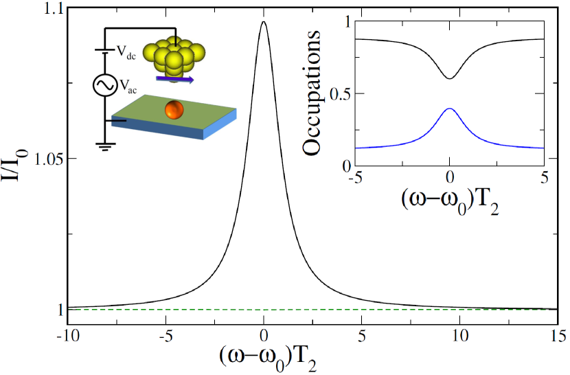
Figure 1: Current detection of STM-ESR. Variation of the DC current as a function of the detuning $\omega-\omega_{0}$ in units of $1/T_{2}$, with $\omega_{0}=(E_{b}-E_{a})/\hbar$ for ${\cal P}_{T}=0.33$ (black) and ${\cal P}_{T}=0$ (green dashed line). The current is given in terms $I_{0}$, the DC current far from resonance. (Left inset) Scheme of the STM-ESR setup: a radiofrequency bias voltage is applied in addition to the DC voltage between the spin-polarized tip and the surface. (Right inset) Variation of the occupation of the ground state, $|a\rangle$, (black) and first excited state, $|b\rangle$, (blue) with detuning. The different parameters are chosen to match the conditions of Fig.3(C) in Baumann et al. Baumann et al. (2015) with $V_{ac}=8$ mV.

III Results

In Sec. II we have sketched the cotunneling mechanism leading to the STM-ESR. In our description, the consequence of the ac driving voltage is summarized in the non-equilibrium occupations $P_{m}(V,\omega)$ and, more explicitly, on the Rabi flop rate $\Omega$, given by Eq.(9). In order to illustrate the results, we make a quite strong simplification: we assume an energy-independent hybridization $V_{\alpha\ell}\equiv V_{\eta,\ell}$ and density of states $\rho_{\eta}(\epsilon)\approx\rho_{\eta}$ and, consequently, we introduce an energy cut-off $E_{c}$. This raw approximation will enable us to estimate the Rabi flop-rate and the ESR current response. By comparing the results with the experimental ones, we show that despite the approximations, the predicted behavior is in qualitative agreement. On the down side, our approach overestimate the Rabi frequency by one order of magnitude.

Below we work out the explicit expressions of the Rabi frequency and we illustrate the main results for two cases, a single orbital Anderson Hamiltonian and the multiorbital case describing the Fe/MgO/Ag(100) system. In the former, the only ingredients are he charging energy of the adatom and the induced Zeeman splitting. In the second case, we describe the magnetic adatom by a multiorbital Hubbard model that includes the Coulomb repulsion between the impurity d-electrons, the crystal field calculated by a point-charge model, Dagotto (2003) the spin-orbit coupling and the Zeeman term. Delgado and Fernández-Rossier (2011); Ferrón et al. (2015) In doing so, we assume hydrogenic-like wavefunctions for the Fe orbitals. The Coulomb interaction is parametrized by a single parameter, the average on-site repulsion $U$. The resulting crystal field depends on two parameters, the expectation values $\langle r^{2}\rangle$ and $\langle r^{4}\rangle$, Dagotto (2003) while the spin-orbit coupling will be defined by its strength $\xi_{SO}$. Despite the quantitative limitations of the point-charge models, they provide a good description of the symmetry of the system and they are very often used to describe ESR spectra. (Abragam and Bleaney, 1970)

III.1 Single-orbital Anderson model

We start discussing the simplest model for a magnetic impurity: the single-orbital Anderson model. This model, which was introduced to describe magnetic impurities on a non-magnetic metal host, Anderson (1966) is equivalent to a single $S=1/2$ spin exchange coupled to conduction electrons. Schrieffer and Wolff (1966) Then, it may be used as an idealization of the STM-ESR experiments on hydrogenated Ti atoms on MgO. Yang et al. (2017); Willke et al. (2018c) The $S=1/2$ spin is isotropic, and the matrix elements $\gamma_{ab}^{m^{\pm}}(\sigma\sigma)$ can be evaluated analytically.

Let us consider that the system is under the influence of a static magnetic field $B_{x}$, so that $|a\rangle$ and $|b\rangle$ are eigenvectors of the spin operator $\hat{S}_{x}$ and $g\mu_{B}B_{x}=\hbar\omega_{0}$ is the Zeeman splitting. Then, assuming that only the tip is spin polarized and using the same notation as in Eq. (9), one gets after some straightforward algebra that $\sum_{\sigma}(1+\sigma{\cal P}_{\eta})\Lambda_{m^{\pm},\eta\sigma}\equiv\mp V_{T}^{2}{\cal P}_{T}\delta_{\eta,T}$, where $V_{T}$ is the hopping between the single level and the tip. In other words, only coupling with a spin-polarized electrode gives a finite contribution to $\Omega$. When the extension of the hybridization function $\Gamma_{T}(E)=2\pi\rho_{T}(E)V_{T}^{2}$, given by the cuttof $E_{c}$, is much larger than the thermal energy $1/\beta$, one gets

$$\Omega\approx\frac{e\Gamma_{T}\left|V_{ac}{\cal P}_{T}\right|}{h|\delta_{ab}|}\left|{\cal I}^{-}(\mu_{-},E_{c},eV)-{\cal I}^{+}(\mu_{+},E_{c},eV)\right|,$$ (12)

where we have approximated the hybridization function $\Gamma_{T}$ by its value at the tip Fermi level, $e$ is the elementary charge and the functions ${\cal I}^{\pm}(\mu_{\pm},E_{c},eV)$ are defined in Appendix B.

Crucially, the result above relies on the fact that the tip polarization is normal to the magnetic field producing the Zeeman splitting, leading to a finite mixing between the eigenvectors $|a\rangle$ and $|b\rangle$. This should not be surprising since in the standard ESR protocols, Abragam and Bleaney (1970) the AC magnetic field is applied perpendicular to a large static field. In our case, the AC electric field yields an effective oscillating magnetic field along the tip polarization direction $z$, which is on resonance with the Zeeman splitting produced by the applied static magnetic field $B_{x}$.

The result (12) has a different reading: the proposed mechanism does not need any particular anisotropy. The key ingredient is thus the effective magnetic field created by the spin-polarized tip, $B^{\rm eff}=2\hbar\Omega/g\mu_{B}$, which is oriented along the tip-polarization direction. In order to have an active ESR signal, this effective field must have a component perpendicular to the the field inducing the Zeeman splitting.

III.1.1 A single-orbital multispin model

In general, transition metal adatoms entails $S\geq 1/2$ spins, and thus, are also subjected to magnetic anisotropy. The dominant interaction with their surroundings takes the form of an exchange coupling,Lorente and Gauyacq (2009); Fernández-Rossier (2009) which determines the IETS, the spin relaxation and decoherence. Delgado and Fernández-Rossier (2017) Hence, the total spin, given by the sum of the local spin and scattering electrons spin, is conserved. Thus, we can model this interaction in the cotunneling context by considering the scattering of the itinerant electrons with a localized magnetic impurity described by a single-orbital state, with a spin $S>1/2$ [multiplicity $(2S+1)$] in its $N_{0}$ electrons state, and spin $S_{\pm}=S-1/2$.  We assume that the states with $N_{0}\pm 1$ electrons are degenerate, which translates into $\Delta E_{m_{\mp}}\mp\mu_{\pm}=\pm\mu_{\pm}$. This description has already been used to describe dynamics and IETS of magnetic adatoms adsorbed on thin insulating layers. Lorente and Gauyacq (2009); Gauyacq et al. (2010) For simplicity, we consider that the $(2S+1)$ states of the system with $N_{0}$ electrons will be equally coupled to the tip and surface states.

The model sketched above allows us us to describe the effective exchange interaction $J_{\alpha\alpha^{\prime}}$ in terms of the transition amplitude operators $\hat{T}_{\pm}(\alpha\alpha^{\prime})$. In addition, it permits relating the Rabi flop rate, Eq. (9), with the local spin $S$. While the energy dependency is the same that appears in the single Anderson model, the crucial differences are associated to $\sum_{m_{\pm},\sigma}(1+\sigma P_{T})\Lambda_{m_{\pm},\alpha}$, see Eq. (10). Using the properties of the Clebsch-Gordan coefficients, one can arrive to Sakurai and Commins (1995)

$$\sum_{m_{\pm},\sigma}(1+\sigma P_{T})\Lambda_{m_{\pm},\alpha}=\frac{P_{T}}{2S(2S+1)}\langle a|\hat{S}_{z}|b\rangle.$$ (13)

Thus, our model predicts a linear dependence with the atomic spin, in good agreement with the observation of STM-ESR weak dependence on the atomic species. Baumann et al. (2015); Natterer et al. (2017); Choi et al. (2017); Willke et al. (2018a, c); Yang et al. (2017); Willke et al. (2018b); Yang et al. (2018)

An important detail of our results is that the Rabi flop rate is proportional to the tip polarization and the hybridization ${\cal P}_{T}\Gamma_{T}$. Hence, it leads to $\Omega\propto I$, which is in apparent contradiction with the experimental observation of a Rabi flop independent of the DC current for the Fe/MgO. Willke et al. (2018a) With this in mind, we examine below the corresponding results based on a multiorbital Hubbard model.

III.2 The Fe/MgO/Ag(100) system

Although STM-ESR has been demonstrated on a variety of magnetic adatoms, Baumann et al. (2015); Natterer et al. (2017); Choi et al. (2017); Willke et al. (2018a, c); Yang et al. (2017); Willke et al. (2018b); Yang et al. (2018) the most studied system is Fe/MgO/Ag(100). Baumann et al. (2015) In a recent work, we have demonstrated that this system can be correctly described by a multiorbital Hubbard model where the crystal and ligand field was estimated from a DFT calculation. Wolf et al. Yet, the results were in qualitative agreement with those obtained with a simpler point-charge model. Wolf et al. ; Baumann (2015) Thus here we use the point charge model results of Ref. [Wolf et al., ].

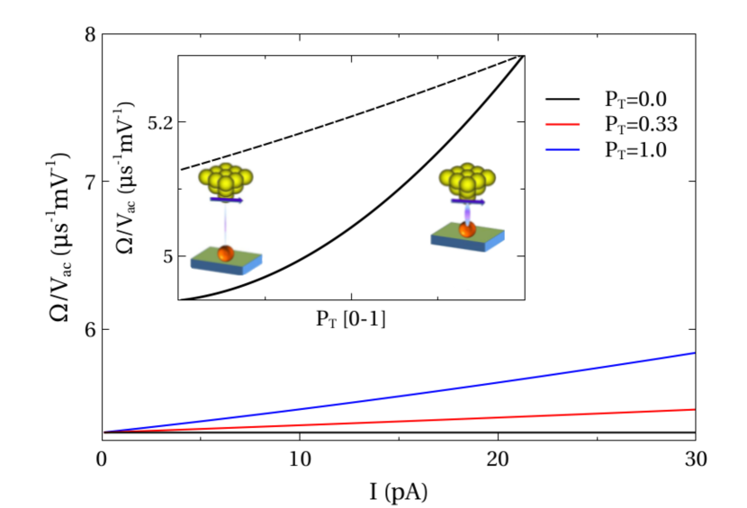
Figure 2: Estimation of $\Omega/V_{ac}$ for the Fe/MgO/Ag(100) system versus the DC current for a constant applied bias voltage $V_{dc}=60$ mV. Each curve corresponds to a different tip polarization ${\cal P}_{T}$. The inset shows the dependence with the tip polarization for the high (thick solid line) and low (thin dashed-line) DC voltages.

For the Ag(100) surface we have Ashcroft and D.Mermin (1976) that $m^{*}=0.99m_{e}$ and $k_{F}\approx\kappa_{F}\approx 1.1$ Å^-1. Typical tunneling current measurements are given in a range where $\kappa L\sim 3-20$, which translates into $|\delta_{ab}^{-1}|\sim(0.3-2.1)\times 10^{-3}$ meV^-1. For simplicity, we assume that all Fe-d orbitals are equally coupled to the substrate, with an energy broadening $\Gamma_{S}\equiv 2\pi\rho_{S}|V_{s}|^{2}$. In the case of coupling to the tip, we assume that only the $d_{z^{2}}$ is actually coupled, as expected from the symmetry of the orbitals, with an induced energy broadening $\Gamma_{T}\propto I$.

In order to check our model, we first take $\Gamma_{S}=2.314$ eV to fit the decoherence time, obtaining $T_{2}=210$ ns for the conditions of Fig. 3C of Ref. [Baumann et al., 2015] at a driving voltage of $8$ mV. Our cotunneling description then predicts a relaxation time $T_{1}$ of the Zeeman-excited state of $T_{1}=8.72$ ms, to be compared with the experimentally determined $T_{1}^{\rm Exp}=88\;\mu$s. The disagreement between both values can have two origins. On one side, we have the limitations due to the oversimplified point-charge model, together with the critical and different dependences of $T_{1}$ and $T_{2}$ on the magnetic anisotropy parameters. On the other side, this transition may also be mediated by the spin-phonon coupling. Paul et al. (2017) Fortunately, our STM-ESR mechanism does not strongly depend on $T_{1}$.

We now turn our attention to the Rabi flop-rate, evaluated according to Eq. (9). The energy integration is done as in Eq. (12), and the only difference comes from the matrix elements $\Lambda_{m^{\pm},\eta\sigma}$. In this case, the sums over $m^{\pm}$ are extended over all states needed to guarantee the convergence. Figure 2 shows the DC current dependence at $V_{dc}=60$ mV of the Rabi flop-rate for three different tip-polarizations: ${\cal P}_{T}=0,\;0.33$ (close to the one estimated experimentally Willke et al. (2018a)) and $1$, the ideal half-metal case. As observed, especially for intermediate polarizations, $\Omega$ is barely affected by the current. This striking result is in agreement with the experimental findings that shows a current-independent Rabi flop rate for currents between 10 pA and 30 pA, Willke et al. (2018a) where authors found that $\Omega/V_{ac}\approx 0.375$ rad.$\mu$s^-1.

The result above points to a crucial ingredient that is not accounted for in the single-orbital Anderson model: the complex orbital structure of the adatom. According to Eq. (10), electrons tunneling into different orbitals $\ell$ of the adatom will lead to unequal contributions to the Rabi flop-rate. The direct consequence is that, contrary to the single-orbital case, the spin averages $\sum_{m_{\pm},\sigma}\Lambda_{m^{\pm},\eta\sigma}$ remains finite, which translates into a finite Rabi flop rate at zero current polarization, see inset of Fig. 3. The weak current dependence appears then as a direct consequence: $\Omega$ contains a fix contribution associated to hybridization with the surface, proportional to $\Gamma_{S}$, and another one of the tip, proportional to $\Gamma_{T}$ ($\propto I$). Since $\Gamma_{S}\gg\Gamma_{T}$ except for very high conductances,Paul et al. (2017) the current independent contribution generally dominates. Comparing the polarization dependence for low voltage, with a current set-point of 0.56 pA at $V_{dc}=5$ mV, and high voltage, with a current of 30 pA at $V_{dc}=60$ mV, we notice that the Rabi frequency is not strongly affected by the dynamics of the excited spin states.

A key issue is the apparent contradiction of our finite Rabi flop-rate for zero-polarization with the observation of the STM-ESR signal only when a spin-polarized tip is used. The solution to this apparent discrepancy is in the detection mechanism of the ESR: current magnetoresistance. This is illustrated in Fig. 1, where we have added the frequency response when a spin-averaging tip is used, assuming exactly the same Rabi flop rate. The resulting steady state current is independent of the frequency and thus, there is not STM-ESR signal.

Willke et al. analyzed in detail the role of the different parameters that controls the STM-ESR. Willke et al. (2018a) In particular, they observed that the resonant peak current saturates with the radio frequency voltage $V_{ac}$, both for small and large set-point currents. In fact, they found that the ratio $I_{\rm peak}/I_{\rm sat}=\psi(V_{ac})$, which they called drive function, was given by $\zeta^{2}/(1+\zeta^{2})$ with $\zeta=V_{ac}/V_{1/2}$, where $V_{1/2}=(T_{1}T_{2})^{-1/2}V_{ac}/\Omega$ is defined as the half-saturation voltage. The relevance of this drive function is that, the larger the drive function, the larger the ESR signal, making the detection more efficient. Thus, we show in Fig. 3a) the drive function obtained from our model, which should be compared with Fig. S2C of Ref. [Willke et al., 2018a]. Our theory correctly reproduce the general trend with the tunnel current. However, due to the overestimation of $T_{1}$ and $\Omega$, our estimated driving function saturates at lower AC bias voltages.

Finally, we would like to call the attention on one point. The experimental observation of the STM-ESR signal requires a finite in-plane magnetic field $B_{x}$. Baumann et al. (2015); Natterer et al. (2017); Choi et al. (2017); Willke et al. (2018a, c); Yang et al. (2017); Willke et al. (2018b); Yang et al. (2018) In Ref. [Baumann et al., 2015], authors argue that this field introduces a mixing between the states $a$ and $b$, the same argument that we exploited in our $S=1/2$ spin model of Sec. III.1. From our expression of the Rabi flop-rate, Eq. (4), we see that its effect is the same as the one produced by a transversal AC magnetic field $B_{\perp}^{\rm eff}=2\hbar\Omega/g\mu_{B}$ on a $S=1/2$ spin system under the action of an static field $B_{\parallel}^{\rm eff}=\hbar\omega_{ba}/g\mu_{B}$.

Hence, the application of a static field that mixes the zero-field states $|a^{0}\rangle$ and $|b^{0}\rangle$, as it is the case of the Fe/MgO, Baumann et al. (2015) and the driving term $\cos(\omega t)\delta H_{\rm cot.}$, leads to the same consequence: a mixing of the low energy states $|a\rangle$ and $|b\rangle$, and thus, to a larger Rabi flop-rate. This is illustrated in Fig. 3b) where we show how $\Omega$ changes with a transversal magnetic field. From the experimental point of view, Baumann et al. (2015); Natterer et al. (2017); Choi et al. (2017); Willke et al. (2018a, c); Yang et al. (2017); Willke et al. (2018b); Yang et al. (2018) the static transversal field $B_{x}$ is also required in order to have a finite tip polarization.

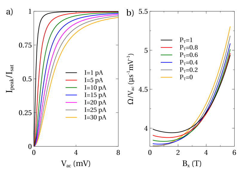
Figure 3: a) Predicted driving function $I_{peak}/I_{sat}$ for the Fe/MgO/Ag(100) system for different currents, to be compared with Ref. [Willke et al., 2018a]. b) Variation of the Rabi flop-rate, $\Omega$, with the external in-plane field $B_{x}$ for different values of tip polarization. The field is applied forming an angle $\theta=3.51\times 10^{-2}$ with the surface plane, with $B_{z}=0.2$ T, while $I=30$ pA and $V_{DC}=60$ mV.

IV Discussion

We have analyzed the effect of an applied radiofrequency bias voltage on the DC tunneling current through a magnetic adatom. Our basic assumption is that this driving voltage leads to a modulation of the tunnel junction transmission with the time-dependent external electric field. In other words, the hopping tunneling amplitudes are modulated, giving place to an off-diagonal time-dependent term in the adatom’s Hamiltonian, which takes the form of the Rabi flop rate.

The amplitude of the modulation was estimated using Bardeen transfer Hamiltonian theory to describe the tunneling current. Bardeen (1961) Thus, we have approximated the potential barrier between the two electrodes, tip and metallic surface, by a square potential. Although the potential in a real STM junction clearly differs from this simple picture, it still can provide results in quantitative agreement. Lounis (2014) A clear improvement over this simple description would be in the form of the Tersoff-Hamann description of tunnel between a surface and a probe tip. Tersoff and Hamann (1985) We should remark that the square-potential approximation only affects the hopping tunnel amplitudes from the tip (or surface) to the magnetic adatom and vice versa. This analysis already reveals an interesting consequence: the more opaque the tunnel junction is, the larger the ESR signal is. This observation is in consonance with the measurement of STM-ESR signals on Ag (100) coated with a thin insulating layer of MgO, Baumann et al. (2015); Natterer et al. (2017); Choi et al. (2017); Willke et al. (2018a, c); Yang et al. (2017); Willke et al. (2018b); Yang et al. (2018) and it opens the possibility of observing ESR signal on similar surfaces, such as Cu₂N/Cu(100). Notice that, since the resonant signal is observed in the tunneling current, a right balance between detectable tunnel currents and opaque character must be reached.

Our description of the tunneling process is based on second-order perturbation theory, which is adequate to describe the behavior of magnetic adsorbates deposited on a thin decoupling layer on top of the metallic substrate, such as MgO on Ag(100),Baumann et al. (2015); Natterer et al. (2017); Choi et al. (2017); Willke et al. (2018a, c); Yang et al. (2017); Willke et al. (2018b); Yang et al. (2018) or Cu₂N. Hirjibehedin et al. (2006); Ternes (2017); Delgado and Fernández-Rossier (2017) The effect of the driving field is summarized in a single parameter: the Rabi flop-rate $\Omega$. Thus, all our efforts have been oriented to estimate $\Omega$. In doing so, we keep a second-order description of the interaction of the quantum system (the adatom) with the electronic baths (surface and tip electrons), using the Bloch-Redfield approach to treat open quantum system. Breuer and Petruccione (2002) In addition, we assume that the small and fast-oscillating driving field does not modified the dissipative dynamics. Cohen-Tannoudji et al. (1998) In this description, the variation of the tunneling amplitudes induced by the radiofrequency potential leads to an oscillating perturbation of the adatom Hamiltonian. This time-dependent contribution mixes the stationary states of the adatom, giving place to a finite Rabi flop-rate.

We have applied our theory on three different models to simulate the STM-ESR mechanism. In first place, to a single-orbital Anderson model, which reveals that isotropic $S=1/2$ systems can be ESR active with a Rabi flop rate proportional to the tip polarization $P_{T}$. A generalization of this model corresponds to a single-orbital multispin system with $S>1/2$, which can also include magnetic anisotropy. Our analysis showed that the resulting Rabi frequency is proportional to the matrix elements $\langle a|\hat{S}_{z}|b\rangle$ of the spin operator between the two states connected by the resonant signal. This finding is in agreement with the observation of similar Rabi flop-rates for different atomic species. Baumann et al. (2015); Natterer et al. (2017); Choi et al. (2017); Willke et al. (2018a, c); Yang et al. (2017); Willke et al. (2018b); Yang et al. (2018) Thus, the proposed mechanism does not rely on a particular symmetry of the adsorbed adatom, neither on the adatom magnetic anisotropy or total spin. This ubiquity is in agreement with the experimental observation of STM-ESR for a variety of adatoms adsorbed on MgO, Baumann et al. (2015); Natterer et al. (2017); Choi et al. (2017); Willke et al. (2018a, c); Yang et al. (2017); Willke et al. (2018b); Yang et al. (2018) including the Ti-H complex behaving as a $S=1/2$ spin. Willke et al. (2018c, b); Yang et al. (2017) This should work also with other spin-$1/2$ systems, including molecules with $S=1/2$ spin centers like the Cu phthalocyanine. A similar analysis should also work for half-integer spins with strong hard-axis anisotropy, for which the ground state doublet satisfy $|\langle S_{z}\rangle|\approx 1/2$.

The resulting Rabi flop-rate depends on off-diagonal matrix elements mixing the two states connected by the ESR, and thus, it can be described as an effective AC magnetic field $B^{\rm eff}_{\perp}=2\hbar\Omega/g\mu_{B}$, whose orientation is parallel to the tip-polarization. This is similar to the usual ESR where the AC field is perpendicular to the field creating the Zeeman splitting, and explains the need of an in-plane magnetic field in the experiments of Baumann et al. Baumann et al. (2015)

One prediction of the single-orbital models is that $\Omega$ is directly proportional to the tip polarization. This leads to a null contribution of the spin-unpolarized surface to the Rabi flop rate, which in turn leads to a linear dependence on current. Although current dependences for $S=1/2$ systems have not been reported to the best of our knowledge, this result is in contrast with the observation of a current-independent Rabi flop rate for Fe/MgO. Willke et al. (2018a) Hence, we employed a more sophisticated description of the adatom in terms of a multiorbital Anderson Hamiltonian derived from a multiplet calculation. Using the well known Fe/MgO system as example, this model already pointed to an important result: when the orbital degrees of freedom of the adatom are accounted for, the modulation of the tunnel barrier by the AC electric field generates a finite Rabi flop rate even in the absence of current polarization. Due to the usually dominant contribution of scattering with surface electrons, the contribution associated to the surface overshadow the (current-dependent) tip part. This result is thus in agreement with the observed weak current dependence. Willke et al. (2018a)

Finally, although we have provided a way to calculate the intensity of the driving term $\Omega$, a quantitative description is challenging: it involves a precise knowledge of the hybridization functions with the surface and tip, together with the density of states. Here we have used a rough estimation based on a flat-band model. Despite the limitations, it allows us to get Rabi flop-rates high enough to explain the observation of ESR signals, but the values are off the experimental ones by a factor 10-20. Willke et al. (2018a) Here two alternative improvements can be envisaged. On one hand, to use the hybridization functions $V_{k;\ell}$ from a Wannier representation of the DFT results, together with the PDOS $\rho(\epsilon)$ on the whole energy interval. This approach is still problematic due to both, slow convergence of the hybridization in the Wannier bases, and the already poor DFT representation of the surface hybridization. Korytár and Lorente (2011) On the other, one could use the flat band approach with constant hybridizations using the cut-off as a fitting parameter. In both cases one finds an additional problem: the most notable contribution is associated to the spin-polarized tip, whose microscopic structure is basically unknown.

Our theory also predicts a finite Rabi flop-rate for spin-unpolarized tunneling currents but, since the detection mechanism is based on magnetoresistance, the DC current is in this case immune to the radiofrequency, in accordance with the experimental observation.

V Conclusions

In this work, we have demonstrated that the all-electrical spin resonance phenomenon can be understood by the modulation of the tunnel junction transmission with the time-dependent external electric field. This, in turns, originates an oscillating driving term on the adatom energy, which can be understood as an effective magnetic field connecting the two states involved in the ESR transition.

Our description is based on a perturbative treatment of the interaction between the adatom and surface and probe tip. In particular, the electric driving field leads to a perturbation of the adatom Hamiltonian, which can be interpreted as an effective transversal magnetic field coupling the eigenstates of the adatom.

The proposed mechanism leads to a Rabi flop-rate barely dependent on the tunneling current, in agreement with the experimental observations for Fe/MgO. Willke et al. (2018a) Likewise, it predicts a linear dependence with the atomic spin component $\hat{S}_{z}$, in good agreement with the observation of STM-ESR weakly dependent on the atomic species. Baumann et al. (2015); Natterer et al. (2017); Choi et al. (2017); Willke et al. (2018a, c); Yang et al. (2017); Willke et al. (2018b); Yang et al. (2018) In addition, it permits us to understand the interplay between the tip-polarization, the magnetic anisotropy and the transversal magnetic field.

Future work involves improving the determination of the hybridizations in order to yield quantitative predictions. Albeit the mentioned problems to calculate the Rabi flop-rate, an accurate description of the ESR-lineshape also involves the relaxation $T_{1}$ and decoherence $T_{2}$ times of the atomic spin. From a theory point of view, a parameter-free description of the ratio $T_{1}/T_{2}$ is really demanding. Both quantities have in general a completely different dependence on the adatom magnetic anisotropy, longitudinal and transverse magnetic fields. Delgado and Fernández-Rossier (2017) Thus, even if we were able to reproduce the excitation spectrum with an uncertainty smaller than $k_{B}T$, the uncertainty in $T_{1}/T_{2}$ would be of several orders of magnitude. As a matter of fact, the extreme energy resolution of STM-ESR together with the time resolution of STM pump-probe techniques can be used to test the different theoretical methods.

Appendix A Review of the cotunneling theory

The tunneling Hamiltonian that changes the number of electrons in the correlated quantum system by one unit can be written as

$${\cal H}_{tun}=\sum_{\alpha,\mathbf{i}}\left[V_{\alpha,\mathbf{i}}(t)f_{\alpha}^{\dagger}d_{\mathbf{i}}+V^{*}_{\alpha,\mathbf{i}}(t)d^{\dagger}_{\mathbf{i}}f_{\alpha}\right]\equiv{\cal V}^{-}(t)+{\cal V}^{+}(t)$$ (14)

where $d^{\dagger}_{\mathbf{i}}$ creates an electron with quantum numbers $\mathbf{i}=(\ell,\sigma)$ with $\ell$ the orbital number and $\sigma=\sigma_{\alpha}$ the spin. Using second-order perturbation theory we can write an effective Hamiltonian acting only on the $N_{0}$-charge space, which hereafter we shall refer as neutral charge state. If we denote by $|M_{\pm}\rangle$ the eigenstates of the decoupled electrode+central region with $N_{0}\pm 1$ electron, we can write the matrix elements between states $|N\rangle$ and $|N^{\prime}\rangle$ as

$$\sum_{M_{-}}\frac{{\cal V}^{+}|M_{-}\rangle\langle M_{-}|{\cal V}^{-}}{E_{M_{-}}-E_{0}}+\sum_{M_{+}}\frac{{\cal V}^{-}|M_{+}\rangle\langle M_{+}|{\cal V}^{+}}{E_{M_{+}}-E_{0}},$$ (15)

where $E_{0}$ is the ground state energy of the (decoupled) system with $N_{0}$ electrons in the central region. Roughly speaking, the cotunneling approach will remain valid as long as

$$\left|\frac{\langle N|{\cal V}^{\pm}|M_{\mp}\rangle}{E_{M_{\mp}}-E_{N}}\right|\ll 1$$ (16)

Now we have to evaluate the corresponding matrix elements. First, let us consider the $|N\rangle$ states can be written as $|N\rangle=|n\rangle\otimes|\Psi\rangle$ where $|\Psi\rangle$ is a multi electronic Slater determinant that describes independent Fermi seas of left and right electrodes. They describe an arbitrary state of the central island and states with an electron-hole pair in the electrodes. For the $N_{0}\pm 1$ electron states, we write $|M_{\pm}\rangle=|m_{\pm}\rangle\otimes|\Psi_{\mp}\rangle$, where now $|\Psi_{\mp}\rangle$ is a Slater state for the electrodes with one electron more (+) or less (-) than the $N_{0}$ manifold.

If we denote by $|0\rangle$ the ground state of the electrodes in the Fermi sea with no excitations in the neutral charge state, we can write $|\Psi\rangle\equiv f_{\alpha}^{\dagger}f_{\alpha}|0\rangle$, where we are creating an electron-hole pair with quantum number $\alpha$. For the states with one electron excess (defect) we will have $|\Psi_{-}\rangle=f_{\beta}f_{\alpha}^{\dagger}f_{\alpha}|0\rangle$ and $|\Psi_{+}\rangle=f_{\beta^{\prime}}^{\dagger}f_{\alpha}^{\dagger}f_{\alpha}|0\rangle$. The zero-temperature occupation of an electrode state $\alpha$ is then given by $n_{\alpha}=\langle\Psi|f_{\alpha}^{\dagger}f_{\alpha}|\Psi\rangle$, which can only take the values 0 or 1 for electrons.

The matrix element of the electrode operator in Eq. (15) selects only one term in the electrode part of the sums $\sum_{M_{\pm}}=\sum_{m_{\pm}}\sum_{\Psi_{\mp}}$. Then one can write

$$\sum_{\Psi_{+}}\langle\Psi|f_{\gamma}|\Psi_{+}\rangle=(1-n_{\gamma})\delta_{\beta\gamma},$$ (17)

$$\sum_{\Psi_{-}}\langle\Psi|f_{\gamma}^{\dagger}|\Psi_{-}\rangle=n_{\gamma}\delta_{\beta\gamma}.$$ (18)

Making the corresponding substitution into Eq. (14) we get

$$\sum_{M_{-}}\frac{\langle N|{\cal V}^{+}|M_{-}\rangle\langle M_{-}|{\cal V}^{-}|N^{\prime}\rangle}{E_{M_{-}}-E_{0}} = \sum_{\alpha\alpha^{\prime}}\left(1-n_{\alpha}\right)$$ (20)

$$\times\langle n|\hat{T}_{-}(\alpha\alpha^{\prime};t)|n^{\prime}\rangle\langle\Psi|f_{\alpha}f_{\alpha^{\prime}}^{\dagger}|\Psi\rangle,$$

and

$$\sum_{M_{+}}\frac{\langle N|{\cal V}^{-}|M_{+}\rangle\langle M_{+}|{\cal V}^{+}|N^{\prime}\rangle}{E_{M_{+}}-E_{0}} = \sum_{\alpha\alpha^{\prime}}n_{\alpha}$$ (22)

$$\langle n|\hat{T}_{+}(\alpha\alpha^{\prime};t)|n^{\prime}\rangle\langle\Psi|f_{\alpha}^{\dagger}f_{\alpha^{\prime}}|\Psi\rangle,$$

where we have introduced the transition amplitude operators $\hat{T}_{\pm}(\alpha\alpha^{\prime};t)$, whose matrix elements are given by

$$\langle n|\hat{T}_{-}(\alpha\alpha^{\prime};t)|n^{\prime}\rangle = \sum_{m_{-},\ell\ell^{\prime}}\frac{V^{*}_{\alpha,\ell}(t)V_{\alpha^{\prime},\ell^{\prime}}(t)}{E_{m_{-}}-E_{0}+\epsilon_{\alpha}}\gamma_{nn^{\prime}}^{m_{-}}(\alpha\ell,\alpha^{\prime}\ell^{\prime})$$ (23)

$$\langle n|\hat{T}_{+}(\alpha\alpha^{\prime};t)|n^{\prime}\rangle = \sum_{m_{+},\ell\ell^{\prime}}\frac{V_{\alpha,\ell}(t)V^{*}_{\alpha^{\prime},\ell^{\prime}}(t)}{E_{m_{+}}-E_{0}-\epsilon_{\alpha}}\gamma_{nn^{\prime}}^{m_{+}}(\alpha\ell,\alpha^{\prime}\ell^{\prime}).$$ (25)

Equations (20)-(22) can be simplified by taking into account that $\sum_{\alpha,\alpha^{\prime}}n_{\alpha}\langle\Psi|f_{\alpha}f_{\alpha^{\prime}}^{\dagger}|\Psi\rangle=\langle\Psi|\sum_{\alpha\alpha^{\prime}}f_{\alpha}f_{\alpha^{\prime}}^{\dagger}|\Psi\rangle$. Hence, when we restrict the reservoir states to single electron-hole pairs $|\Psi\rangle$, we recover Eq. (8) of the main text.

Notice that here, the central region is described by a time-independent Hamiltonian ${\cal H}_{C}$ and thus, stationary eigenvalues and eigenvectors can be introduced without loss of generality. If, on the other hand, the time dependence is contained in ${\cal H}_{C}$, the stationary description becomes ill defined. Despite this issue, a similar analysis can be carried out provided the driving field is small enough. For instance, if the central region is under the effect of a time-dependent electric potential $|V_{ac}|\ll|E_{m_{\pm}}-E_{0}|$, we can still work in the pseudo-stationary states $|N\rangle$ and $|M_{\pm}\rangle$, while the energy differences becomes

$$E_{m_{\pm}}(t)-E_{0}(t)\approx E_{m_{\pm}}-E_{0}\mp V_{ac}\cos(\omega t).$$ (27)

Appendix B Energy integrals ${\cal I}^{\pm}(z_{1},Ec,z_{2})$

The following energy integrals can be done analytically by deformation in the complex energy plane

$${\cal I}^{\pm}(\epsilon_{0},E_{c},\mu)={\cal P}\int_{-E_{c}}^{E_{c}}d\epsilon\frac{f^{\pm}_{\mu}(\epsilon)}{\epsilon_{0}-\epsilon}.$$ (28)

The results are given by

$${\cal I}^{+}(\epsilon_{0},E_{c},\mu)\approx \ln(2\pi)-\ln(E_{c}-\mu+\epsilon_{0})$$ (30)

$$+{\rm Re}\left[\psi^{(0)}\left(\frac{1}{2}-\frac{i(\epsilon_{0}-\mu)}{2\pi}\right)\right],$$

and

$${\cal I}^{-}(\epsilon_{0},E_{c},\mu)\approx\ln\left|\frac{\epsilon_{0}-E_{c}}{\epsilon_{0}+E_{c}}\right|-{\cal I}^{+}(\epsilon_{0},E_{c},\mu).$$ (31)

where $\psi^{(0)}(x)$ is the digamma function and the arguments satisfy $-\epsilon_{0}+\mu<E_{c}<\epsilon_{0}-\mu$. The above approximations correspond to asymptotic expansions for $E_{c}\gg 1$. Notice that here we have used a description in terms of dimensionless variables, which is equivalent to measure all energies in units of $k_{B}T$. In the case of interest, $E_{c}\gg 1$ and $E_{c}/\epsilon_{0}\sim 1$. In this limit, to lowest order in $1/E_{c}$, we have that

$${\cal I}^{\pm}(\epsilon_{0},E_{c},\mu)\sim\mp\ln\left(\frac{1}{1+\epsilon_{0}/E_{c}}\right).$$ (32)

References

- Baumann et al. (2015) S. Baumann, W. Paul, T. Choi, C. P. Lutz, A. Ardavan, and A. J. Heinrich, Science 350, 417 (2015).
- Müllegger et al. (2014) S. Müllegger, S. Tebi, A. K. Das, W. Schöfberger, F. Faschinger, and R. Koch, Phys. Rev. Lett. 113, 133001 (2014), URL https://link.aps.org/doi/10.1103/PhysRevLett.113.133001.
- Müllegger et al. (2015) S. Müllegger, E. Rauls, U. Gerstmann, S. Tebi, G. Serrano, S. Wiespointner-Baumgarthuber, W. G. Schmidt, and R. Koch, Phys. Rev. B 92, 220418 (2015), URL https://link.aps.org/doi/10.1103/PhysRevB.92.220418.
- Willke et al. (2018a) P. Willke, W. Paul, F. D. Natterer, K. Yang, Y. Bae, T. Choi, J. Fernández-Rossier, A. J. Heinrich, and C. P. Lutz, Science Advances 4 (2018a), eprint http://advances.sciencemag.org/content/4/2/eaaq1543.full.pdf.
- Loth et al. (2010a) S. Loth, M. Etzkorn, C. P. Lutz, D. M. Eigler, and A. J. Heinrich, Science 329, 1628 (2010a).
- Paul et al. (2017) W. Paul, K. Yang, S. Baumann, N. Romming, T. Choi, C. P. Lutz, and A. J. Heinrich, Nature Physics 13, 403 (2017).
- Choi et al. (2017) T. Choi, W. Paul, S. Rolf-Pissarczyk, A. J. Macdonald, F. D. Natterer, K. Yang, P. Willke, C. P. Lutz, and A. J. Heinrich, Nature nanotechnology 12, 420 (2017).
- Willke et al. (2018b) P. Willke, K. Yang, Y. Bae, A. Heinrich, and C. P. Lutz (2018b), arXiv:1807.08944.
- Natterer et al. (2017) F. D. Natterer, K. Yang, W. Paul, P. Willke, T. Choi, T. Greber, A. J. Heinrich, and C. P. Lutz, Nature 543, 226 (2017).
- Yang et al. (2017) K. Yang, Y. Bae, W. Paul, F. D. Natterer, P. Willke, J. L. Lado, A. Ferrón, T. Choi, J. Fernández-Rossier, A. J. Heinrich, et al., Phys. Rev. Lett. 119, 227206 (2017), URL https://link.aps.org/doi/10.1103/PhysRevLett.119.227206.
- Willke et al. (2018c) P. Willke, Y. Bae, K. Yang, J. L. Lado, A. Ferrón, T. Choi, A. Ardavan, J. Fernández-Rossier, A. J. Heinrich, and C. P. Lutz, Science 362, 336 (2018c), ISSN 0036-8075, eprint http://science.sciencemag.org/content/362/6412/336.full.pdf, URL http://science.sciencemag.org/content/362/6412/336.
- Yang et al. (2018) K. Yang, P. Willke, Y. Bae, A. Ferrón, J. L. Lado, A. Ardavan, J. Fernández-Rossier, A. J. Heinrich, and C. P. Lutz, Nature nanotechnology 13, 1120 (2018).
- Berggren and Fransson (2016) P. Berggren and J. Fransson, Scientific reports 6, 25584 (2016).
- Lado et al. (2017) J. L. Lado, A. Ferrón, and J. Fernández-Rossier, Phys. Rev. B 96, 205420 (2017), URL https://link.aps.org/doi/10.1103/PhysRevB.96.205420.
- Shakirov et al. (2018) A. M. Shakirov, A. N. Rubtsov, and P. Ribeiro (2018), arXiv:1806.08260.
- Chudnovsky et al. (2005) E. M. Chudnovsky, D. A. Garanin, and R. Schilling, Phys. Rev. B 72, 094426 (2005), URL https://link.aps.org/doi/10.1103/PhysRevB.72.094426.
- Calero and Chudnovsky (2007) C. Calero and E. M. Chudnovsky, Physical Review Letters 99 (2007), ISSN 0031-9007, 1079-7114, URL https://link.aps.org/doi/10.1103/PhysRevLett.99.047201.
- (18) J. Reina, C. Wolf, F. Delgado, and N. Lorente, unpublished. A homogeneous electric field leads to a zero rotational of the phonon deformation field and thus to a zero spin-phonon coupling.
- Note (1) Note1, although in the first work on ESR, Baumann et al. (2015) there was not resonant signal on Co, authors have confirmed us that it can also be detected.
- Bardeen (1961) J. Bardeen, Phys. Rev. Lett. 6, 57 (1961).
- Lorente and Persson (2000) N. Lorente and M. Persson, Physical Review Letters 85, 2997 (2000), URL http://link.aps.org/doi/10.1103/PhysRevLett.85.2997.
- Lorente (2004) N. Lorente, Applied Physics A 78, 799 (2004), ISSN 0947-8396, 1432-0630, URL http://link.springer.com/10.1007/s00339-003-2434-8.
- Jauho et al. (1994) A. P. Jauho, N. S. Wingreen, and Y. Meir, Phys. Rev. B. 50, 5528 (1994).
- Note (2) Note2, if the occupations are assumed to change with time, the total number of electrons in the contact is no longer conserved, leading to a charge pileup in the contacts. In addition, it also originates an instantaneous loss of phase coherence in the contacts Jauho et al. (1994).
- Taurian and Springborg (1985) O. Taurian and N. Springborg, M.and Christensen, Solid State Communications 55, 351 (1985).
- Ternes (2015) M. Ternes, New Journal of Physics 17, 063016 (2015).
- Delgado and Fernández-Rossier (2017) F. Delgado and J. Fernández-Rossier, Progress in Surface Science 92, 40 (2017).
- Breuer and Petruccione (2002) H.-P. Breuer and F. Petruccione, The theory of open quantum systems (Oxford University Press, 2002).
- Cohen-Tannoudji et al. (1998) C. Cohen-Tannoudji, G. Grynberg, and J. Dupont-Roc, Atom-Photon Interactions (Wiley and Sons, INC., New York, 1998).
- Hofer et al. (2017) P. P. Hofer, M. Perarnau-Llobet, L. D. M. Miranda, G. Haack, R. Silva, J. B. Brask, and N. Brunner, New Journal of Physics 19, 123037 (2017).
- González et al. (2017) J. O. González, L. A. Correa, G. Nocerino, J. P. Palao, D. Alonso, and G. Adesso, Open Systems & Information Dynamics 24, 1740010 (2017).
- Stano et al. (2015) P. Stano, J. Klinovaja, F. R. Braakman, L. M. K. Vandersypen, and D. Loss, Phys. Rev. B 92, 075302 (2015), URL https://link.aps.org/doi/10.1103/PhysRevB.92.075302.
- Anderson (1966) P. W. Anderson, Phys. Rev. Lett. 17, 95 (1966).
- Schrieffer and Wolff (1966) J. R. Schrieffer and P. A. Wolff, Phys. Rev. 149, 491 (1966).
- (35) C. Wolf, J. Reina, F. Delgado, and N. Lorente, Spin hamiltonian of Fe on MgO, in preparation.
- Note (3) Note3, tip is usually made of W, but indentation may lead to different apex atoms, while metallic substrate is Ag(100).
- Messiah (1999) A. Messiah, Quantum Mechanics (Dover, New York, 1999).
- (38) M. R. Wegewijs and Y. V. Nazarov, arXiv:cond-mat/0103579.
- Delgado and Fernández-Rossier (2011) F. Delgado and J. Fernández-Rossier, Phys. Rev. B 84, 045439 (2011).
- Note (4) Note4, in the Bloch-Redfield theory, there are other terms of the Redfield tensor proportional to the coherences that may also contribute to the current. Breuer and Petruccione (2002) However, they involve rates coupling coherences with occupations, which are usually quite small and will be discarded here.
- Delgado et al. (2010) F. Delgado, J. J. Palacios, and J. Fernández-Rossier, Phys. Rev. Lett. 104, 026601 (2010).
- Loth et al. (2010b) S. Loth, K. von Bergmann, M. Ternes, A. F. Otte, C. P. Lutz, and A. J. Heinrich, Nature Physics 6, 340 (2010b).
- Dagotto (2003) E. Dagotto, Nanoscale Phase Separation and Colossal Magnetoresistance (Springer-Verlag, Berlin, 2003).
- Ferrón et al. (2015) A. Ferrón, F. Delgado, and J. Fernández-Rossier, New J. Phys. 17, 033020 (2015).
- Abragam and Bleaney (1970) A. Abragam and B. Bleaney, Electron Paramagnetic Resonance of Transition Ions (Oxford University Press, Oxford, 1970).
- Note (5) Note5, notice that the spin-dependent excitation energy in the denominators of Eq. (9) can be neglected when the addition energy is very large.
- Lorente and Gauyacq (2009) N. Lorente and J.-P. Gauyacq, Phys. Rev. Lett. 103, 176601 (2009).
- Fernández-Rossier (2009) J. Fernández-Rossier, Phys. Rev. Lett. 102, 256802 (2009).
- Note (6) Note6, the spin of the electrons state could be either or . However, the conclusions are not affect by this change.
- Gauyacq et al. (2010) J.-P. Gauyacq, F. D. Novaes, and N. Lorente, Phys. Rev. B 81, 165423 (2010), URL https://link.aps.org/doi/10.1103/PhysRevB.81.165423.
- Sakurai and Commins (1995) J. J. Sakurai and E. D. Commins, Modern quantum mechanics, revised edition (Addison Wesley, Massachusetts, 1995), pp. 214–216.
- Baumann (2015) S. Baumann, Ph.D. thesis, University_of_Basel (2015), URL http://edoc.unibas.ch/diss/DissB_11597.
- Ashcroft and D.Mermin (1976) N. W. Ashcroft and N. D.Mermin, Solid State Physics (Thomson Learning, 1976).
- Lounis (2014) S. Lounis, ArXiv:1404.0961 (2014).
- Tersoff and Hamann (1985) J. Tersoff and D. R. Hamann, Phys. Rev. B 31, 805 (1985).
- Hirjibehedin et al. (2006) C. F. Hirjibehedin, C. P. Lutz, and A. J. Heinrich, Science 312, 1021 (2006).
- Ternes (2017) M. Ternes, Progress in Surface Science 92, 83 (2017), ISSN 0079-6816, URL http://www.sciencedirect.com/science/article/pii/S0079681617300011.
- Korytár and Lorente (2011) R. Korytár and N. Lorente, Journal of Physics: Condensed Matter 23, 355009 (2011), ISSN 0953-8984, 1361-648X, URL http://iopscience.iop.org/0953-8984/23/35/355009.