Quasi-normal modes in a symmetric triangular barrier

Abstract

Quasi-normal modes (QNMs) of the massless scalar wave in $1+1$ dimensions are obtained for a symmetric, finite, triangular barrier potential. This problem is exactly solvable, with Airy functions involved in the solutions. Before obtaining the QNMs, we demonstrate how such a triangular barrier may arise in the context of scalar wave propagation in a tailor-made wormhole geometry. Thereafter, the Ferrari-Mashhoon idea is used to show how bound states in a well potential may be used to find the QNMs in a corresponding barrier potential. The bound state condition in the exactly solvable triangular well and the transformed condition for finding the QNMs are written down. Real bound state energies and complex QNMs are found by solving the respective transcendental equations. Numerical integration of the wave equation yields the time domain profiles for scalar waves propagating in this wormhole geometry which illustrate the quasinormal ringing. Estimates relating the size of the wormhole throat (in units of solar mass) with the QNM frequencies are stated and discussed. Finally, we show how the effective potential and the QNMs for scalar perturbations of the Ellis–Bronnikov wormhole spacetime can be reasonably well–approximated using a properly parametrised triangular barrier.

I INTRODUCTION

An oft-quoted example of the quasinormal mode is the ringing sound we hear when we strike a metal glass with a metallic rod. The ringing decays in time–thus the mode is quasi-normal and not a usual normal mode. The decay of the ringing obviously means that energy is lost in the environment –the system is open and hence dissipative. In many ways, such systems are interesting and also realistic.

The earliest mention and discussion on such modes appear in the paper in 1900 by Horace Lamb lamb who calls them peculiar vibrations, while analysing the wave system arising in the free vibrations of a nucleus in an extended medium. Much of the early work on these modes (and also quite a bit of the later work as well) are thus in nuclear physics.

In the late fifties, the main governing equations for gravitational perturbations of black holes (eg. the Schwarzschild) were derived in the context of the stability of the Schwarzschild spacetime in the seminal paper by Regge and Wheeler regge . Much later, Zerilli zerilli obtained the effective potential for even-parity perturbations. However, it was in 1970, in an article published in the journal Nature Vishveshwara , Vishveshwara first noted the quasi-normal mode in gravitational physics, while working on perturbations of black holes Vishveshwara1 . Following soon, came the work of Chandrasekhar and Detweiler in 1975 Chandrasekhar , wherein, among other issues concerning the Schwarzschild black hole, the exact quasinormal modes in a toy model of the rectangular barrier potential was discussed. Several other potentials also exhibit exact quasinormal modes (eg. Poschl-Teller PT ,PT1 ), which have been found and analysed in detail, over the years. A fairly comprehensive list of such potentials and their quasi-normal spectra can be found in visser .

In the current wake of detection of gravitational waves Ligo1 the study of quasi-normal modes has received renewed interest. Such modes arise in the context of black hole stability and are discussed extensively in black hole perturbation theory. Since there is loss of energy involved, the quasi-normal frequency must be complex with the real part giving the actual energy carried by the wave and the imaginary part giving an idea about the damping time. One must have the right sign for the imaginary part in order to have a decay in the time domain profile. In astrophysics, the QNMs are important because they depend only on the source/system parameters (eg. mass, angular momentum etc.) and not on the cause producing them. This can help us in obtaining information about the parameters of a black hole or even a wormhole aneesh . Through the nature of the solutions for the scalar or tensor QNMs, one can differentiate various theories of gravity f(R) .

The central problem lies in calculating the modes. In most cases, the wave equation is not exactly solvable due to the complexity of the effective potential. Numerical methods are the only way out. Though various semi-analytical techniques, like the WKB method WKB are there to provide a physical intuition on the behavior of these modes, to get precise values, one has to use different numerical techniques. The handful of scenarios where exact solutions are possible are limited and therefore important. Such exact solutions, if not of any real value (in the sense of observations), do have great utility in a pedagogic sense, to say the very least. As mentioned before, apart from the square barrier, there are several other potentials for which exact expressions for the modes are available visser . In our work here, we study another simple example–the case of a symmetric, finite, triangular barrier.

The triangular barrier potential and its inverse (the triangular well) are exactly solvable potentials whose solutions are found in terms of the Airy functions ghatak . The knowledge of the bound states of the potential (in terms of Airy functions) shows the way towards finding the QNMs, using an interesting correspondence first found by Ferrari and Mashhoon mashhoon1 ; mashhoon2 ; ferrari ; blome . The Ferrari-Mashhoon method shows how a given barrier potential, via a change of variables and parameters, can be inverted into a well potential, in which bound states can be found. Using the inverse transformation, one can extract the QNMs too, including the spatial wave functions. The QNMs which are obtained from inverse transformation of the bound state eigenvalues are termed as the proper quasi-normal modes. However, the QNMs can also be found by directly using the appropriate boundary conditions and without referring to the corresponding bound-state problem in an inverted (well) potential. Despite being an interesting idea, the Ferrari-Mashhoon correspondence has limited applicability in finding QNMs, largely because of its reliance on the knowledge of the solution of the associated bound state problem.

Our work here is organised as follows. In Section II we briefly introduce the potential well and also the barrier on which our work is based. Also, in this section we construct a wormhole solution morris whose effective potential for scalar wave propagation is a triangular barrier. In Section III, we discuss the idea of quasi-normal modes and explain the Ferrari-Mashhoon correspondence. Section IV deals with the bound states of the symmetric, finite triangular well and the corresponding energy eigenvalues. Section V is devoted to QNMs of the triangular barrier. Here we first find the QNMs using the Ferrari-Mashhoon idea and then mention how the QNMs can also be obtained independently. Thereafter, we numerically solve the wave equation and obtain the time-domain profiles at a fixed value of the spatial coordinate. In order to get some idea about numbers, we calculate the frequency and corresponding damping time for different throat radii of the wormhole. Finally, we show how the effective potential of the well-known Ellis–Bronnikov spacetime ellis can be well-approximated by a triangular barrier. Section VI is a summary with some comments on the results obtained and possible implications and extensions. A short conclusion appears in Section VII.

II TRIANGULAR WELL AND BARRIER POTENTIALS

The symmetric, finite triangular potential well is given as,

$$\mathrm{V(x)}=\begin{cases}\mathrm{\frac{V_{0}|x|}{a}-V_{0}}&;\,\,\mathrm{-a\leq x\leq a}\\ 0&;\,\,\mathrm{x>a,x<-a\,},\end{cases}$$ (1)

where $2a$ is width of the well and $V_{0}$ is the depth of the well. In order to get the corresponding potential barrier we invert the above potential,

$$\mathrm{V(x)}=\begin{cases}\mathrm{V_{0}-\frac{V_{0}|x|}{a}}&;\,\,\mathrm{-a\leq x\leq a}\\ 0&;\,\,\mathrm{x>a,x<-a\,}.\end{cases}$$ (2)

Figures 1(a) and 1(b) show the triangular well and the triangular barrier, respectively.

Let us now see where, and in which context, a triangular barrier potential may arise. It is a known fact that the effective potentials for scalar wave propagation in wormhole geometries morris have single or double barrier features. For example, in Ellis-Bronnikov geometry ellis the effective potential is a single barrier. Can we have a wormhole geometry for which the effective potential is a triangular barrier? To address and answer this question, we do some reverse engineering. We write down the scalar wave equation in a spacetime with one unknown function $r(x)$. Thereafter we obtain the $r(x)$ for which we have a wormhole.

To begin, let us assume the line element to be of the form:

$$\mathrm{ds^{2}=-dt^{2}+dx^{2}+r^{2}(x)(d\theta^{2}+sin^{2}\theta d\phi^{2}),}$$ (3)

where the coordinate $x$ ($-\infty\leq x\leq\infty$) is like the ‘tortoise’ coordinate commonly used in black hole physics and the radial coordinate $r$ is written in terms of $x$ through the relation

$$\mathrm{dx^{2}=g_{rr}{dr^{2}}\,}.$$ (4)

The only unknown function in the line element is $r(x)$ which, for a wormhole, is symmetric, $r(x)=r(-x)$. Also, $r(x=0)$ is finite, positive and non-zero. In addition, for asymptotic flatness, we usually assume that $r\rightarrow\pm x$ as $x$ becomes large. However, in our example below, we will see that $r(x)$ will tend to $\pm x$ at a finite $x$, exactly where the triangular barrier will end and the potential will become zero. In other words, we have a wormhole ‘sandwiched’ between two flat regions.

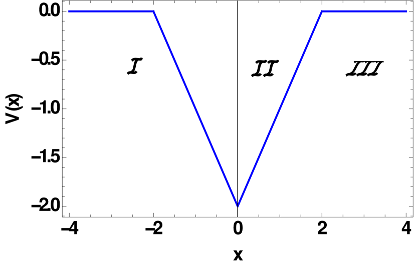
(a) Potential well

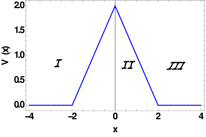
(b) Potential barrier

Figure 1: $V_{0}=a=2$

If we intend to study the propagation of a massless scalar wave in such a spacetime we need to solve the Klein-Gordon equation, given as:

$$\Box\Phi=0\,.$$ (5)

After separation of variables using the ansatz

$$\mathrm{\Phi(x,t,\theta,\phi)=u(x)\,e^{-i\omega t}\,Y(\theta\,,\phi)}$$ (6)

and writing the radial equation, we get

$$\mathrm{\frac{d^{2}u}{dx^{2}}+\frac{2r^{\prime}}{r}\frac{du}{dx}+\Big{(}\omega^{2}-\frac{m(m+1)}{r^{2}}\Big{)}u=0\,},$$ (7)

where the prime denotes a derivative w.r.t. $x$. $m$ is related to the angular momentum. To find the effective potential, we rewrite equation (7) in the form of the time-independent Schrödinger equation, by eliminating the first order derivative term with a change of the dependent variable. Thus, assuming $u(x)=A(x)B(x)$ and considering the differential equation for $A(x)$, we note that for the first derivative in $A(x)$ term to vanish, we need $B(x)$ to satisfy

$$\mathrm{\frac{B^{\prime}}{B}=-\frac{r^{\prime}}{r}}.$$ (8)

Substituting this in equation $(7)$ we find the equation for $A(x)$ to be

$$\mathrm{\frac{A^{\prime\prime}}{A}+\Big{(}\omega^{2}-\frac{m(m+1)}{r^{2}}-\frac{r^{\prime\prime}}{r}\Big{)}=0\,}.$$ (9)

Hence the effective potential is given as,

$$\mathrm{V(x)=\frac{m(m+1)}{r(x)^{2}}+\frac{r^{\prime\prime}(x)}{r(x)}\,}.$$ (10)

If we want the effective potential for the $m=0$ mode to be a symmetric triangular barrier as shown in Figure $1(b)$ then,

$$\mathrm{\frac{r^{\prime\prime}}{r}}=\begin{cases}\mathrm{V_{0}-\frac{V_{0}|x|}{a}}&\mathrm{,-a\leq x\leq a}\\ 0&\mathrm{,x>a,x<-a\,}.\end{cases}$$ (11)

On solving the above equation we get $r(x)$ given as,

$$\mathrm{r(x)}=\begin{cases}\mathrm{-x}&\mathrm{,x<-a}\\ \mathrm{C\,Ai\Big{[}\frac{V_{0}\,+\frac{V_{0}x}{a}}{(\frac{V_{0}}{a})^{\frac{2}{3}}}\Big{]}+D\,Bi\Big{[}\frac{V_{0}\,+\frac{V_{0}x}{a}}{(\frac{V_{0}}{a})^{\frac{2}{3}}}\Big{]}}&\mathrm{,-a\leq x\leq 0}\\ \\ \mathrm{C\,Ai\Big{[}\frac{V_{0}\,-\frac{V_{0}x}{a}}{(\frac{V_{0}}{a})^{\frac{2}{3}}}\Big{]}+D\,Bi\Big{[}\frac{V_{0}\,-\frac{V_{0}x}{a}}{(\frac{V_{0}}{a})^{\frac{2}{3}}}\Big{]}}&\mathrm{,0\leq x\leq a}\\ \mathrm{x}&\mathrm{,x>a}\end{cases}$$ (12)

where Ai and Bi are the Airy functions of first and second kind respectively and $C$ and $D$ are constants. For the regions $x>a$ and $x<-a$ the spacetime is flat and $V(x)=0$. The metric in these two regions is Minkowskian. One may note that the differential equation for region $0\leq x\leq a$ will have a general solution with the argument of the Airy function being $\frac{V_{0}-\frac{V_{0}x}{a}}{(\frac{-V_{0}}{a})^{\frac{2}{3}}}$. Since we require $r(x)$ to be a continuous function over the entire region, we take only one root of $(-1)^{\frac{1}{3}}$ i.e. -1, which, when squared becomes 1. The other two roots of $(-1)^{\frac{1}{3}}$, which we do not use, correspond to Airy functions having factors $e^{\frac{\pm 2i\pi}{3}}$ in the argument.
We need to ensure that the function $r(x)$ thus constructed, is continuous and so is its first derivative across the boundary. This requirement will lead to the following two matching conditions:

$$\mathrm{C\,Ai[0]+D\,Bi[0]=a}$$ (13)

$$\mathrm{C\,Ai^{\prime}[0]+D\,Bi^{\prime}[0]=-\Big{(}\frac{V_{0}}{a}\Big{)}^{\frac{-1}{3}}\,}.$$ (14)

Taking the ratio of the above equations we obtain,

$$\mathrm{\frac{C}{D}=-\frac{zBi^{\prime}[0]+Bi[0]}{zAi^{\prime}[0]+Ai[0]}}$$ (15)

where $z=(V_{0}a^{2})^{\frac{1}{3}}$.

Since we wish to construct a wormhole geometry, $r(x=0)$ cannot be zero. Hence we must consider the even set of solutions for which $r^{\prime}(x=0)=0$. Imposing this condition we find,

$$\mathrm{\frac{C}{D}=-\frac{Bi^{\prime}[z]}{Ai^{\prime}[z]}\,}.$$ (16)

Thereafter, combining equations $(15)$ and $(16)$, we arrive at a transcendental equation of the form-

$$\mathrm{\frac{Bi^{\prime}[z]}{Ai^{\prime}[z]}=\frac{zBi^{\prime}[0]+Bi[0]}{zAi^{\prime}[0]+Ai[0]}}.$$ (17)

Solving the above equation, gives the value of $z=1.58377$.
This value imposes a condition on $V_{0}$ and $a$ given as,

$$\mathrm{z=(V_{0}a^{2})^{\frac{1}{3}}=1.58377}$$ (18)

which, in turn implies that the $m=0$ mode effective potential of the scalar wave (spatial part) is a symmetric triangular barrier.
The constants $C$ and $D$ have the dimension of length due to the overall factor ‘$a$’ present in their expressions. Solving equations $(13)$ and $(14)$ we obtain,

$$\mathrm{C\,=a\,{\frac{Bi^{\prime}[0]+\frac{1}{z}Bi[0]}{Ai[0]Bi^{\prime}[0]-Ai^{\prime}[0]Bi[0]}}\,=a{\frac{0.44+\frac{1}{z}0.61}{0.318}}}$$ (19)

$$\mathrm{D\,=a\,{\frac{Ai^{\prime}[0]+\frac{1}{z}Ai[0]}{Ai^{\prime}[0]Bi[0]-Ai[0]Bi^{\prime}[0]}}\,=a{\frac{-0.26+\frac{1}{z}0.35}{-0.318}}\,}.$$ (20)

Finally, we arrive at the expression of $r(x)$ given as,

$$\mathrm{r(x)}=\begin{cases}\mathrm{-x}&\mathrm{,x<-a}\\ \mathrm{a{\frac{0.44+\frac{1}{z}0.61}{0.318}}\,Ai\Big{[}\frac{V_{0}\,+\frac{V_{0}x}{a}}{(\frac{V_{0}}{a})^{\frac{2}{3}}}\Big{]}+a{\frac{-0.26+\frac{1}{z}0.35}{-0.318}}\,Bi\Big{[}\frac{V_{0}\,+\frac{V_{0}x}{a}}{(\frac{V_{0}}{a})^{\frac{2}{3}}}\Big{]}}&\mathrm{,-a\leq x\leq 0}\\ \\ \mathrm{a{\frac{0.44+\frac{1}{z}0.61}{0.318}}\,Ai\Big{[}\frac{V_{0}\,-\frac{V_{0}x}{a}}{(\frac{V_{0}}{a})^{\frac{2}{3}}}\Big{]}+a{\frac{-0.26+\frac{1}{z}0.35}{-0.318}}\,Bi\Big{[}\frac{V_{0}\,-\frac{V_{0}x}{a}}{(\frac{V_{0}}{a})^{\frac{2}{3}}}\Big{]}}&\mathrm{,0\leq x\leq a}\\ \mathrm{x}&\mathrm{,x>a.}\end{cases}$$ (21)

In order to visualise the wormhole geometry, let us consider $V_{0}=a$. Thus, $V_{0}=a=z=1.58377$, which gives the values of the constants as $C=4.16233$ and $D=0.172416$. The throat radius $(b_{0})$ of the wormhole thus constructed, is given as:

$$\mathrm{b_{0}\,=r(x=0)=a\Big{(}{\frac{0.44+\frac{1}{z}0.61}{0.318}}Ai[z]+{\frac{-0.26+\frac{1}{z}0.35}{-0.318}}Bi[z]\Big{)}=a(0.39098)\,=0.619222\,.}$$ (22)

Note that the throat radius depends only on $a$ since $z$ is already fixed. Hence one can choose a $b_{0}$ which will lead to fixed values of $a$ and $V_{0}$.

The plot below (Figure 2) shows the behavior of $r(x)$ with respect to $x$ for the above values of $V_{0}$ and $a$. It should be noted that the second derivative of $r(x)$ is discontinuous which is reflected in the fact that the wormhole we constructed has matter only in the region $-a\leq x\leq a$. Beyond $x=a,-a$, the metric is that of flat spacetime. At the boundaries, the curvature tensors have a discontinuity reminiscent of the construction of a ‘sandwich’ spacetime.

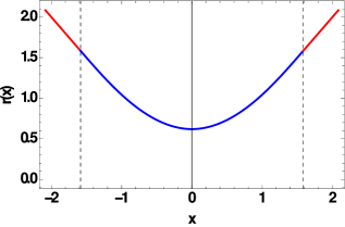
Figure 2: Variation of $r(x)$

We can obtain the energy– momentum tensor corresponding to this wormhole and try to understand the nature of matter contained in the region $-a\leq x\leq a$. From the Einstein equations of General Relativity (using $8\pi G=c=1$) and the Einstein tensor for the above-stated line element, we get (equating $T_{00}=\rho(x)$, $T_{11}=\tau(x)$, $T_{22}=T_{33}=p(x)$, as defined in the frame basis),

$$\mathrm{\rho(x)=-\frac{2r(x)r^{\prime\prime}(x)+r^{\prime}(x)^{2}-1}{r(x)^{2}}}$$ (23)

$$\mathrm{\tau(x)=\frac{r^{\prime}(x)^{2}-1}{r(x)^{2}}}$$ (24)

$$\mathrm{p(x)=\frac{r^{\prime\prime}(x)}{r(x)}.}$$ (25)

In the above, one needs to use the expression for $r(x)$ obtained in equation (21) for the region $-a\leq x\leq a$. For any possible value of $a$ and $V_{0}$ the energy density will be a negative quantity. If we take the case $a=V_{0}=1.58377$, then at the throat, $\rho(x=0)=-0.559$ in appropriate units. Therefore, as expected morris , exotic matter, violating the Weak Energy Condition (WEC), is required to support this wormhole too.

III QUASINORMAL MODES AND BOUND STATES

III.1 Quasi-normal modes

Quasi-normal modes are a discrete set of complex frequencies which satisfy the boundary conditions of purely outgoing waves at $x\rightarrow\mp\infty$, for an open system Vishveshwara ; cardoso . To find the QNMs in a given problem we begin with the standard $1+1$ dimensional wave equation in the presence of a potential $V(x)$, i.e. we have

$$\mathrm{\frac{\partial^{2}\phi}{\partial t^{2}}-\frac{\partial^{2}\phi}{\partial x^{2}}+V(x)\phi=0\,.}$$ (26)

Using $\mathrm{\phi(t,x)=e^{-i\omega t}\psi(x)}$, the spatial wave function $\psi(x)$ obeys a time-independent Schrödinger equation:

$$\mathrm{\frac{d^{2}\psi(x)}{dx^{2}}+(E-V(x))\psi(x)=0\hskip 14.45377pt\longrightarrow\hskip 14.45377pt\frac{d^{2}\psi(x)}{dx^{2}}+(\omega^{2}-V(x))\psi(x)=0\,.}$$ (27)

The coordinate $x$ is a spatial coordinate ranging from $-\infty$ to $+\infty$ and $E=\omega^{2}$. Time $t$ runs from $0$ to infinity. The equation for $\psi(x)$ needs to be solved with proper outgoing boundary conditions at the spatial infinities, if $\omega$ is to represent a complex quasi-normal frequency. The corresponding $\phi(x,t)$ is the quasi-normal mode with $\mathrm{\phi(x,t)=e^{-i\omega t}\psi(x)}$. For an asymptotically flat, static spacetime, the potential is positive and satisfies,

$$\mathrm{V(x)\rightarrow 0\hskip 21.68121ptas\hskip 21.68121ptx\rightarrow\pm\infty}$$ (28)

with the boundary conditions being:

$$\mathrm{\psi\rightarrow e^{-i\omega x}\hskip 14.45377ptas\hskip 14.45377ptx\rightarrow-\infty\hskip 21.68121ptand\hskip 21.68121pt\psi\rightarrow e^{i\omega x}\hskip 14.45377ptas\hskip 14.45377ptx\rightarrow\infty\,.}$$ (29)

For a black hole spacetime this is physically motivated and makes sense as at the horizon $x\rightarrow-\infty$, there shall only be an ingoing wave, while at spatial infinity $x\rightarrow\infty$ there will only be the outgoing wave carrying the energy away from the system to infinity. Note that for $\omega$ with a negative imaginary part, the time part $e^{-i\omega t}$ behaves like a damped oscillation and the spatial part diverges to infinity. Thus, the meaningful use of the QNMs appears to be through the nature of the temporal part. The spatial part is evaluated at fixed $x$ (finite) and its equation, when solved, yields the QNMs.

III.2 Ferrari-Mashhoon method: a bound state–quasinormal mode correspondence

In their 1984 paper, Ferrari and Mashhoonmashhoon2 ; ferrari devised a new analytical technique for finding the QNMs of black hole spacetimes. The method was based on the fact that there is a connection between the QNMs and the bound states of the inverted potentials mashhoon1 ; mashhoon2 ; ferrari ; blome . Let us begin with the time independent Schrödinger equation for finding the bound states ($E<0$) of a potential well defined by $-V(x,p)$, where $p$ is some parameter appearing in the potential.

$$\mathrm{-\frac{d^{2}\psi}{dx^{2}}-V(x,p)\psi=-E\psi\hskip 14.45377pt\longrightarrow\hskip 14.45377pt\frac{d^{2}\psi}{dx^{2}}+V(x,p)\psi=E\psi}$$ (30)

The bound state wavefunction and the corresponding frequency also depends on the parameter $p$, $\psi=\psi(x,p)$ and $\omega=\omega(p)$.
Consider the transformation

$$\mathrm{x\longrightarrow-ix\hskip 14.45377ptand\hskip 14.45377ptp\longrightarrow p^{\prime}}$$ (31)

such that the potential remains invariant

$$\mathrm{V(x,p)=V(-ix,p^{\prime}).}$$ (32)

The equation $(30)$ under this transformation becomes-

$$\mathrm{\frac{d^{2}\psi}{dx^{2}}\,\longrightarrow\,-\frac{d^{2}\psi}{dx^{2}}\hskip 7.22743pt;\,\frac{d^{2}\psi}{dx^{2}}-V(-ix,p^{\prime})\psi=-E\psi\hskip 7.22743pt=>-\frac{d^{2}\psi}{dx^{2}}+V(x,p)\psi=E\psi}$$ (33)

which is nothing but a time-independent Schrödinger equation for scattering states from a potential barrier $V(x,p)$. Thus, the method says that if we can find a formula for bound state energy, then the QNMs can be obtained from the bound states just by using the transformation in (31). We will later see that for the triangular potential $p^{\prime}=-ip$, which is a special case.

The QNMs found using the correspondence must satisfy the proper boundary conditions. To see this, let us take a look at the Schrödinger equation for the potential well when $V=0$ (i.e. outside the well) given as,

$$\mathrm{\frac{d^{2}\psi}{dx^{2}}-E\psi=0\,.}$$ (34)

The solution is,

$$\mathrm{\psi(x,p)\propto e^{\pm\omega x}\hskip 14.45377pt;x\longrightarrow\mp\infty\,.}$$ (35)

If we use the transformation $x\longrightarrow-ix$ then this solution becomes

$$\mathrm{\psi\propto e^{\mp i\omega x}\hskip 14.45377ptas\hskip 14.45377ptx\longrightarrow\mp\infty}$$ (36)

which is the boundary condition for QNMs. One can also check this by including the time part and writing the full wave function $\phi(t,x)$.

IV BOUND STATES OF THE TRIANGULAR WELL

In order to find the bound states ($E<0$), let us consider, as shown in Figure $1(a)$, three regions: region I for $-\infty<x<-a$, region II for $-a\leq x\leq a$ and region III for $a<x<\infty$.

IV.1 Solving the Schrödinger equation

Region I:

The Schrödinger equation is given as,

$$\mathrm{\frac{d^{2}\psi}{dx^{2}}-E\psi=0\hskip 7.22743pt=>\hskip 7.22743pt\frac{d^{2}\psi}{dx^{2}}-\omega^{2}\psi=0}$$ (37)

where we have taken $\frac{2m}{\hbar^{2}}=1$ and $\omega=\sqrt{E}$. The solution is given by,

$$\mathrm{\psi(x)=Ae^{\omega x}}$$ (38)

with A being a constant. $\psi$ remains finite and tends to zero as $x\,\rightarrow\,-\infty$.

Region III:

The Schrödinger equation remains the same as in Region I with the solution being,

$$\mathrm{\psi(x)=Be^{-\omega x}\,,}$$ (39)

B being some arbitrary constant which has to be equal to the constant A for $\psi$ to be symmetric or anti-symmetric. $\psi$ remains finite and tends to zero as $x\,\rightarrow\,\infty$.

Region II:

The equation in this region is given as

$$\mathrm{\frac{d^{2}\psi}{dx^{2}}}=\begin{cases}\mathrm{\Big{(}\frac{V_{0}x}{a}+E-V_{0}\Big{)}\psi}&;\mathrm{\,\,0\leq x\leq a}\\ \\ \mathrm{\Big{(}-\frac{V_{0}x}{a}+E-V_{0}\Big{)}\psi}&;\,\,\mathrm{-a\leq x\leq 0.}\end{cases}$$ (40)

The above equation is the Airy differential equation with its general solution given as,

$$\mathrm{\psi(x)}=\begin{cases}\mathrm{C\,Ai\Big{[}\frac{\frac{V_{0}x}{a}+E-V_{0}}{(\frac{V_{0}}{a})^{\frac{2}{3}}}\Big{]}+D\,Bi\Big{[}\frac{\frac{V_{0}x}{a}+E-V_{0}}{(\frac{V_{0}}{a})^{\frac{2}{3}}}\Big{]}}&;\,\,\mathrm{0\leq x\leq a}\\ \\ \mathrm{CAi\Big{[}\frac{\frac{-V_{0}x}{a}+E-V_{0}}{(\frac{V_{0}}{a})^{\frac{2}{3}}}\Big{]}+D\,Bi\Big{[}\frac{\frac{-V_{0}x}{a}+E-V_{0}}{(\frac{V_{0}}{a})^{\frac{2}{3}}}\Big{]}}&;\,\,\mathrm{-a\leq x\leq 0}\\ \end{cases}$$ (41)

where $C$ and $D$ are constants and $Ai$, $Bi$ are the Airy functions of first and second kind respectively. Following the argument mentioned in Section II for equation (12) here also we take only one root of $(-1)^{1/3}$ i.e. -1 and squaring it gives 1 in the denominator of the argument of the Airy functions for the solution of $-a\leq x\leq 0$.

IV.2 Constructing even states and matching at boundary

The even states are constructed from the above solution as follows:

$$\mathrm{\psi(x)}=\begin{cases}\mathrm{Ae^{\omega x}}&;\,\,\mathrm{x<-a}\\ \mathrm{C\,Ai\Big{[}\frac{\frac{-V_{0}x}{a}+E-V_{0}}{(\frac{V_{0}}{a})^{\frac{2}{3}}}\Big{]}+D\,Bi\Big{[}\frac{\frac{-V_{0}x}{a}+E-V_{0}}{(\frac{V_{0}}{a})^{\frac{2}{3}}}\Big{]}}&;\,\,\mathrm{-a\leq x\leq 0}\\ \\ \mathrm{C\,Ai\Big{[}\frac{\frac{V_{0}x}{a}+E-V_{0}}{(\frac{V_{0}}{a})^{\frac{2}{3}}}\Big{]}+D\,Bi\Big{[}\frac{\frac{V_{0}x}{a}+E-V_{0}}{(\frac{V_{0}}{a})^{\frac{2}{3}}}\Big{]}}&;\,\,\mathrm{0\leq x\leq a}\\ \mathrm{Ae^{-\omega x}}&;\,\,\mathrm{x>a}\,.\end{cases}$$ (42)

Since the wavefunction and its derivative are continuous over the entire region, we match $\psi$ and $\psi^{\prime}$ across $x=a$,

$$\mathrm{Ae^{-\omega a}=\,C\,Ai\Big{[}\frac{E}{(\frac{V_{0}}{a})^{\frac{2}{3}}}\Big{]}\,+\,D\,Bi\Big{[}\frac{E}{(\frac{V_{0}}{a})^{\frac{2}{3}}}\Big{]}}$$ (43)

$$\mathrm{-\omega Ae^{-\omega a}=\,\Big{(}\frac{V_{0}}{a}\Big{)}^{\frac{1}{3}}\,\Big{(}C\,Ai^{\prime}\Big{[}\frac{E}{(\frac{V_{0}}{a})^{\frac{2}{3}}}\Big{]}\,+\,D\,Bi^{\prime}\Big{[}\frac{E}{(\frac{V_{0}}{a})^{\frac{2}{3}}}\Big{]}\Big{)}\,}.$$ (44)

Hence, by taking the ratio of equations $(43)$ and $(44)$ we get

$$\mathrm{\frac{C}{D}}=\mathrm{-\frac{Bi\Big{[}\frac{E}{(\frac{V_{0}}{a})^{\frac{2}{3}}}\Big{]}+(\frac{1}{\sqrt{E}})\,(\frac{V_{0}}{a})^{\frac{1}{3}}\,Bi^{\prime}\Big{[}\frac{E}{(\frac{V_{0}}{a})^{\frac{2}{3}}}\Big{]}}{Ai\Big{[}\frac{E}{(\frac{V_{0}}{a})^{\frac{2}{3}}}\Big{]}+(\frac{1}{\sqrt{E}})\,(\frac{V_{0}}{a})^{\frac{1}{3}}\,Ai^{\prime}\Big{[}\frac{E}{(\frac{V_{0}}{a})^{\frac{2}{3}}}\Big{]}}\,.}$$ (45)

Since the coefficients $C$ and $D$ are undetermined, we use another condition. For an even wavefunction, $\psi^{\prime}(0)=0$. We have to explicitly apply this condition as our wavefunctions are not inherently symmetric or anti-symmetric. Applying this we get the ratio $\frac{C}{D}$ as

$$\mathrm{\frac{C}{D}=-\frac{Bi^{\prime}\Big{[}\frac{E-V_{0}}{(\frac{V_{0}}{a})^{\frac{2}{3}}}\Big{]}}{Ai^{\prime}\Big{[}\frac{E-V_{0}}{(\frac{V_{0}}{a})^{\frac{2}{3}}}\Big{]}}\,.}$$ (46)

Hence the final transcendental equation, the roots of which are the even bound state energies, is given as,

$$\mathrm{\frac{Bi\Big{[}\frac{E}{(\frac{V_{0}}{a})^{\frac{2}{3}}}\Big{]}+(\frac{1}{\sqrt{E}})\,(\frac{V_{0}}{a})^{\frac{1}{3}}\,Bi^{\prime}\Big{[}\frac{E}{(\frac{V_{0}}{a})^{\frac{2}{3}}}\Big{]}}{Ai\Big{[}\frac{E}{(\frac{V_{0}}{a})^{\frac{2}{3}}}\Big{]}+(\frac{1}{\sqrt{E}})\,(\frac{V_{0}}{a})^{\frac{1}{3}}\,Ai^{\prime}\Big{[}\frac{E}{(\frac{V_{0}}{a})^{\frac{2}{3}}}\Big{]}}=\frac{Bi^{\prime}\Big{[}\frac{E-V_{0}}{(\frac{V_{0}}{a})^{\frac{2}{3}}}\Big{]}}{Ai^{\prime}\Big{[}\frac{E-V_{0}}{(\frac{V_{0}}{a})^{\frac{2}{3}}}\Big{]}}\,.}$$ (47)

IV.3 Constructing odd states and matching at boundary

The odd states are constructed as follows

$$\mathrm{\psi(x)}=\begin{cases}\mathrm{-Ae^{\omega x}}&\mathrm{,x<-a}\\ \mathrm{-C\,Ai\Big{[}\frac{\frac{-V_{0}x}{a}+E-V_{0}}{(\frac{V_{0}}{a})^{\frac{2}{3}}}\Big{]}-D\,Bi\Big{[}\frac{\frac{-V_{0}x}{a}+E-V_{0}}{(\frac{V_{0}}{a})^{\frac{2}{3}}}\Big{]}}&\mathrm{,-a\leq x\leq 0}\\ \\ \mathrm{C\,Ai\Big{[}\frac{\frac{V_{0}x}{a}+E-V_{0}}{(\frac{V_{0}}{a})^{\frac{2}{3}}}\Big{]}+D\,Bi\Big{[}\frac{\frac{V_{0}x}{a}+E-V_{0}}{(\frac{V_{0}}{a})^{\frac{2}{3}}}\Big{]}}&\mathrm{,0\leq x\leq a}\\ \mathrm{Ae^{-\omega x}}&\mathrm{,x>a\,.}\end{cases}$$ (48)

Proceeding in a way similar to the case for even states, we match the wavefunction and its derivative at the boundary to get,

$$\mathrm{\frac{C}{D}=-\frac{Bi\Big{[}\frac{E}{(\frac{V_{0}}{a})^{\frac{2}{3}}}\Big{]}+(\frac{1}{\sqrt{E}})\,(\frac{V_{0}}{a})^{\frac{1}{3}}\,Bi^{\prime}\Big{[}\frac{E}{(\frac{V_{0}}{a})^{\frac{2}{3}}}\Big{]}}{Ai\Big{[}\frac{E}{(\frac{V_{0}}{a})^{\frac{2}{3}}}\Big{]}+(\frac{1}{\sqrt{E}})\,(\frac{V_{0}}{a})^{\frac{1}{3}}\,Ai^{\prime}\Big{[}\frac{E}{(\frac{V_{0}}{a})^{\frac{2}{3}}}\Big{]}}\,.}$$ (49)

Here, since we have odd states, to determine the ratio $\frac{C}{D}$ we evaluate $\psi(0)=0$ which gives,

$$\mathrm{\frac{C}{D}=-\frac{Bi\Big{[}\frac{E-V_{0}}{(\frac{V_{0}}{a})^{\frac{2}{3}}}\Big{]}}{Ai\Big{[}\frac{E-V_{0}}{(\frac{V_{0}}{a})^{\frac{2}{3}}}\Big{]}}\,.}$$ (50)

Hence the final transcendental equation for odd bound state energies becomes,

$$\mathrm{\frac{Bi\Big{[}\frac{E}{(\frac{V_{0}}{a})^{\frac{2}{3}}}\Big{]}+(\frac{1}{\sqrt{E}})\,(\frac{V_{0}}{a})^{\frac{1}{3}}\,Bi^{\prime}\Big{[}\frac{E}{(\frac{V_{0}}{a})^{\frac{2}{3}}}\Big{]}}{Ai\Big{[}\frac{E}{(\frac{V_{0}}{a})^{\frac{2}{3}}}\Big{]}+(\frac{1}{\sqrt{E}})\,(\frac{V_{0}}{a})^{\frac{1}{3}}\,Ai^{\prime}\Big{[}\frac{E}{(\frac{V_{0}}{a})^{\frac{2}{3}}}\Big{]}}=\frac{Bi\Big{[}\frac{E-V_{0}}{(\frac{V_{0}}{a})^{\frac{2}{3}}}\Big{]}}{Ai\Big{[}\frac{E-V_{0}}{(\frac{V_{0}}{a})^{\frac{2}{3}}}\Big{]}}\,.}$$ (51)

IV.4 Finding even and odd eigenvalues and eigenfunctions

In order to obtain representative values for the energies and show their respective wave functions, we consider the following special cases: $\frac{V_{0}}{a}>1$, $\frac{V_{0}}{a}<1$ and $\frac{V_{0}}{a}=1$. The energy eigenvalues are listed below in Table I with the normalised wavefunctions shown in Figure 3 for $V_{0}=5\,,a=2$.

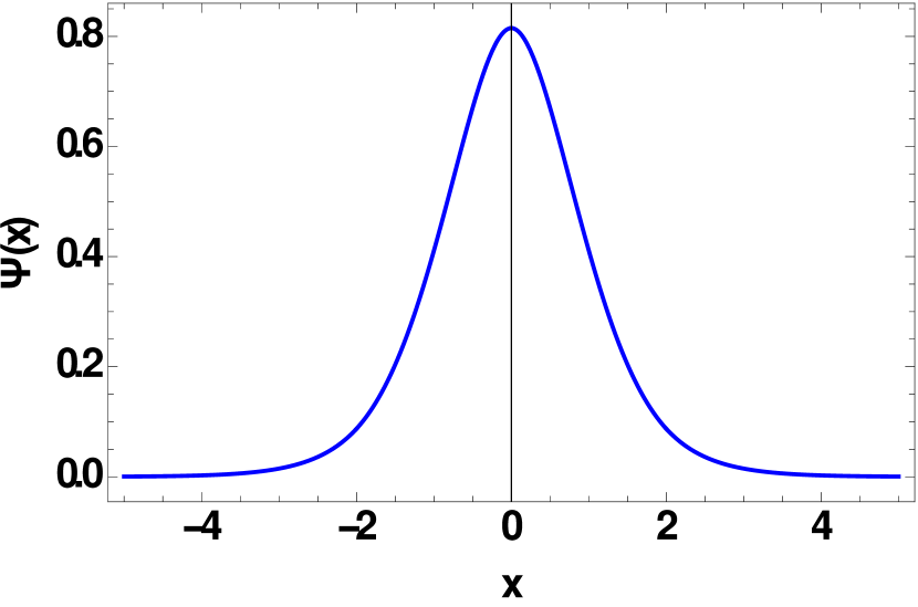
(a) Even state of $V_{0}=5,a=2$

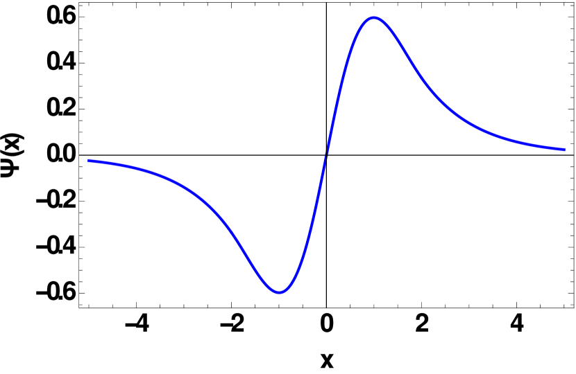
(b) Odd state of $V_{0}=5,a=2$

Figure 3: Normalised wavefunction for $V_{0}=5,a=2$.

	Even state	Odd state
$V_{0}=a=2$	0.99364	0.000266614
$V_{0}=5,a=2$	3.12575	0.775377
$V_{0}=2,a=5$	0.254455	0.731984
$V_{0}=a=1$	0.173819	No odd state

Table 1: Energy eigenvalues for even and odd states.

V FINDING THE QUASI-NORMAL MODES

Let us now move on towards finding the QNMs in the barrier potential. Using the Ferrari-Mashhoon idea we define a transformation which will keep the potential unchanged. This transformation is given as,

$$\mathrm{x\,\longrightarrow\,-ix\,.}$$ (52)

which changes the sign of the second derivative term in the time-indepenedent Schrodinger equation. This results in the well becoming a barrier. In our case, the potential remains invariant since $a\longrightarrow-ia$. The solutions for the different regions can be obtained from the bound states by simply imposing the transformation mentioned above. One may find the QNMs directly by solving the Schrödinger equation for a barrier with proper QNM boundary conditions. However, since our potential is invariant under the transformation $(52)$ one can also get the QNMs by making use of the Ferrari-Mashhoon method. It is important to note that while doing so, one must keep in mind that we need to consider only $(i)^{\frac{1}{3}}=-i$ as the other roots of $(i)^{1/3}$ can be absorbed by considering $e^{\frac{\pm 2i\pi}{3}}$ in the argument of the Airy function and remembering that they do not give any new solution DLMF . Thus the even set of solutions in the three regions of the barrier (Fig. 1b) become

$$\mathrm{\psi(x)}=\begin{cases}\mathrm{Ae^{-i\omega x}}&;\,\,\mathrm{x<-a}\\ \mathrm{C\,Ai\Big{[}\frac{\frac{V_{0}x}{a}-E+V_{0}}{(\frac{V_{0}}{a})^{\frac{2}{3}}}\Big{]}+D\,Bi\Big{[}\frac{\frac{V_{0}x}{a}-E+V_{0}}{(\frac{V_{0}}{a})^{\frac{2}{3}}}\Big{]}}&;\,\,\mathrm{-a\leq x\leq 0}\\ \\ \mathrm{C\,Ai\Big{[}\frac{\frac{-V_{0}x}{a}-E+V_{0}}{(\frac{V_{0}}{a})^{\frac{2}{3}}}\Big{]}+D\,Bi\Big{[}\frac{\frac{-V_{0}x}{a}-E+V_{0}}{(\frac{V_{0}}{a})^{\frac{2}{3}}}\Big{]}}&;\,\,\mathrm{0\leq x\leq a}\\ \mathrm{Ae^{i\omega x}}&;\,\,\mathrm{x>a}\,.\end{cases}$$ (53)

For the odd set of wavefunctions there will be a negative sign in the amplitude of $\psi(x)$ in the region $-\infty<x<0$. The quasi-normal modes for the even and odd states are obtained by solving the transcendental equations $(55)$ and $(56)$ (see below) respectively which have been obtained by imposing the transformation on equations $(47)$ and $(51)$. In the argument of the Airy functions of equations (47) and (51) we impose $a\rightarrow-ia$ which gives $(i)^{2/3}$. As mentioned earlier we take $(i)^{1/3}=-i$ and squaring it gives $-1$. Thus, we have,

$$\mathrm{\frac{E}{(\frac{V_{0}}{a})^{\frac{2}{3}}}\xrightarrow{a\rightarrow-ia}\frac{-E}{(\frac{V_{0}}{a})^{\frac{2}{3}}}.}$$ (54)

Also the factor of $(\frac{V_{0}}{a})^{1/3}$ provides the additional factor of $i$ multiplied with $\sqrt{E}$. Hence we get the following transcendental equations as

$$\mathrm{\frac{Bi\Big{[}\frac{-E}{(\frac{V_{0}}{a})^{\frac{2}{3}}}\Big{]}+(\frac{1}{i\sqrt{E}})\,(\frac{V_{0}}{a})^{\frac{1}{3}}\,Bi^{\prime}\Big{[}\frac{-E}{(\frac{V_{0}}{a})^{\frac{2}{3}}}\Big{]}}{Ai\Big{[}\frac{-E}{(\frac{V_{0}}{a})^{\frac{2}{3}}}\Big{]}+(\frac{1}{i\sqrt{E}})\,(\frac{V_{0}}{a})^{\frac{1}{3}}\,Ai^{\prime}\Big{[}\frac{-E}{(\frac{V_{0}}{a})^{\frac{2}{3}}}\Big{]}}=\frac{Bi^{\prime}\Big{[}\frac{V_{0}-E}{(\frac{V_{0}}{a})^{\frac{2}{3}}}\Big{]}}{Ai^{\prime}\Big{[}\frac{V_{0}-E}{(\frac{V_{0}}{a})^{\frac{2}{3}}}\Big{]}}}$$ (55)

$$\mathrm{\frac{Bi\Big{[}\frac{-E}{(\frac{V_{0}}{a})^{\frac{2}{3}}}\Big{]}+(\frac{1}{i\sqrt{E}})\,(\frac{V_{0}}{a})^{\frac{1}{3}}\,Bi^{\prime}\Big{[}\frac{-E}{(\frac{V_{0}}{a})^{\frac{2}{3}}}\Big{]}}{Ai\Big{[}\frac{-E}{(\frac{V_{0}}{a})^{\frac{2}{3}}}\Big{]}+(\frac{1}{i\sqrt{E}})\,(\frac{V_{0}}{a})^{\frac{1}{3}}\,Ai^{\prime}\Big{[}\frac{-E}{(\frac{V_{0}}{a})^{\frac{2}{3}}}\Big{]}}=\frac{Bi\Big{[}\frac{V_{0}-E}{(\frac{V_{0}}{a})^{\frac{2}{3}}}\Big{]}}{Ai\Big{[}\frac{V_{0}-E}{(\frac{V_{0}}{a})^{\frac{2}{3}}}\Big{]}}}$$ (56)

for even and odd QNMs, respectively.

V.1 Solving the transcendental equations

In order to find the roots of the transcendental equations (55) and (56) we do a contour plot in Mathematica 10.0 mathematica by equating the real and imaginary parts of LHS and RHS so that the intersection points will give us the initial guess for the quasinormal frequencies. Next we use the FindRoot command in Mathematica 10.0 to explicitly find the numerical value of the root using an initial guess obtained from the contour plot. In the table below (Table II) some of the QNM frequencies are mentioned for different values of the parameters in the potential. The plot in Figure 4 shows the even and odd QNM wavefunctions for the $V_{0}=a=1.58377$ which we had obtained in Section II. Thus the QNMs shown in Figure 4 will also be the QNMs for a wormhole geometry under scalar perturbation for the $m=0$ mode.

	Even states	Odd states
$V_{0}=a=2$	$1.37818-i\,0.377625$	$1.84536-i\,0.916893$
$V_{0}=5,a=2$	$2.08866-i\,0.323045$	$2.32235-i\,0.723801$
	$2.92932-i\,0.947045$	$3.62696-i\,1.17254$
$V_{0}=2,a=5$	$1.2607-i\,0.184607$	$1.2408-i\,0.263773$
	$1.43577-i\,0.252766$	$1.66907-i\,0.367693$
$V_{0}=a=1.58377$	$1.21957-i\,0.58865$	$2.03544-i\,1.40477$

Table 2: Values of $\omega_{QNM}$ for different potentials.

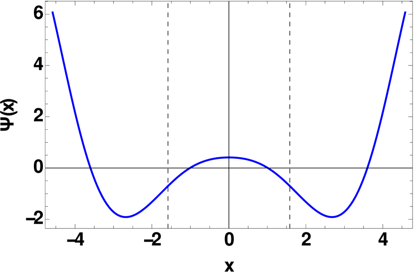
(a) Even QNM

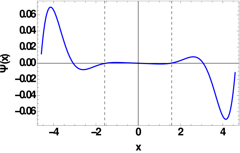
(b) Odd QNM

Figure 4: QNMs for $V_{0}=a=1.58377$.

V.2 The time domain profile

The time domain profile of a wave function satisfying a given wave equation, shows its evolution with time at a particular value of spatial position. The time domain profile can also be used to obtain the QNM frequencies as described in price and konoplya . It is found by directly integrating the wave-like equation (26) and observing the behavior of the field, at a particular spatial coordinate, with time. The entire time domain profile comprises of the initial transient phase, followed by the QNM ringing (during the ringdown phase) and, finally, the late time behavior. In order to generate such a profile we first write equation (26) in light cone coordinates $du=dt-dx$ and $dv=dt+dx$. This gives,

$$\mathrm{\Big{(}4\frac{\partial^{2}}{\partial u\partial v}+V(u,v)\Big{)}\phi=0.}$$ (57)

The time evolution operator in light cone coordinates can be written as,

$$\begin{split}\mathrm{exp\Big{(}h\frac{\partial}{\partial t}\Big{)}=exp\Big{(}h\frac{\partial}{\partial u}+h\frac{\partial}{\partial v}\Big{)}=exp\Big{(}h\frac{\partial}{\partial u}\Big{)}+exp\Big{(}h\frac{\partial}{\partial v}\Big{)}-1}\\ \mathrm{+\frac{h^{2}}{2}\Big{(}exp\Big{(}h\frac{\partial}{\partial u}\Big{)}+exp\Big{(}h\frac{\partial}{\partial v}\Big{)}\Big{)}\frac{\partial^{2}}{\partial u\partial v}+....}\end{split}$$ (58)

When this operates on $\phi$ and incorporating (57), we get the discretised form of the differential equation with step size $h$ given as:

$$\mathrm{\phi(u+h,v+h)=\phi(u+h,v)+\phi(u,v+h)-\phi(u,v)-\frac{h^{2}}{8}V(u,v)(\phi(u,v+h)+\phi(u+h,v))+.....}$$ (59)

We integrate along each cell of a $uv$ grid bounded by two null surfaces $u=u_{0}$ and $v=v_{0}$ with $h=0.1$. The initial conditions on the $v=0$ line is a Gaussian profile centered at $u=10$, i.e. $\psi(u,0)=e^{\frac{-(u-10)^{2}}{100}}$. On the $u=0$ line $\psi$ is taken as a constant, $\psi(0,v)=constant$, the value of which is determined by the value of $\psi(0,0)$. The field is obtained in the region $0<u<150$ and $0<v<150$. We then obtain $\phi(t)$ for a particular value of the spatial coordinate. This is plotted in a logarithmic scale as a function of time. The scheme is elegantly described in konoplya .

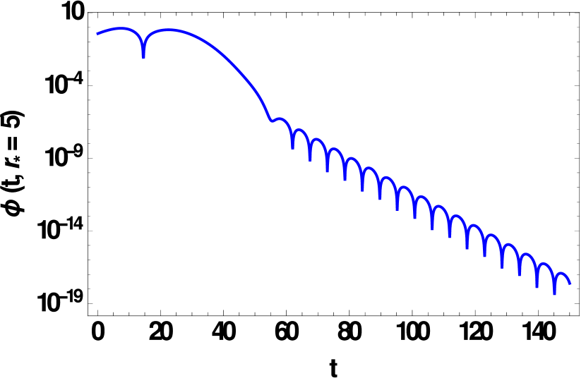
(a) $V_{0}=0.3412$ and $a=3.412$

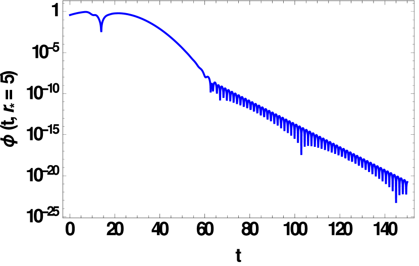
(b) $V_{0}=5$ and $a=2$

Figure 5: Time domain profiles showing quasi-normal ringing.

$V_{0}$	a	$\omega$ (analytical)	$\omega$ (Prony)
$0.3412$	$3.412$	0.56607 -i 0.27322	0.566933 -i 0.272709
$1.5837$	$1.5837$	1.21957 -i 0.58865	1.22222 -i 0.587214
$7.3512$	$0.73512$	2.62748 -i 1.2682	2.62767 -i 1.26129
$1$	$10$	0.95141 -i 0.081617	0.951777 -i 0.0831705
$2$	$5$	1.2607 -i 0.184607	1.266 -i 0.187367
$2$	$2$	1.37818 -i 0.377625	1.37844 -i 0.377593
$4$	$4$	1.9608 -i 0.247561	1.96429 -i 0.249405
$5$	$2$	2.08866 -i 0.323045	2.08925 -i 0.325319

Table 3: Values of QNM frequencies for different $V_{0}$ and $a$.

Figure 5 shows the time-domain profiles obtained by integrating the wave equation with a triangular barrier potential using the method mentioned above. We observe that the QNM ringing is quite prominent and the amplitude decays with time during this phase. The values of the dominant frequency extracted from the time domain profile matches quite well with the fundamental QNM frequency obtained analytically for different $V_{0}$ and $a$, as is indicated in Table III. The extraction of frequencies from the time domain profile is done by applying the Prony fitting technique where the QNM spectrum is written as a superposition of damped exponentials konoplya . Even though our potential has a derivative discontinuity, we still found the fundamental QNM frequency dominating the time evolution of the field nollert . For the first three values in Table III, we have taken values of $V_{0}$ and $a$ such that relation (18) is satisfied, giving us the time domain profile for scalar wave propagation in the ‘sandwich’ wormhole constructed in section II and the corresponding QNM frequencies. The plot of Fig. 5(a) clearly shows the decaying nature of the scalar field during the QNM ringing phase. Fig 5(b) shows the time domain profile for other values of the $V_{0}$ and $a$ (not obeying (18)). The plot in Figure 5(a) demonstrates that the wormhole we have constructed is stable w.r.t. scalar perturbations. We can also generalize our comment and state that any spacetime having a perturbation potential in the form of a triangular barrier is likely to be be stable under scalar perturbations.

V.3 Variation of the QNMs with the wormhole throat radius

The QNM frequencies have the special characteristic that they depend only on the parameters of the source, like for a black hole the only parameters are its mass, charge and spin. In our wormhole scenario, the parameters are the potential height $V_{0}$ and the width of the potential barrier $2a$ which in turn control the throat radius $b_{0}$ of the wormhole constructed by us as given in equation (22). Thus, in order to observe how the QNM frequencies change for a real physical wormhole (assuming wormholes exist in nature) we need to observe the dependence of the frequency and damping time of the signal on the throat radius. For simplicity, let us consider only the fundamental modes of the even states. If we take the throat radius in units of solar mass $(M_{\odot})$, we get the $\omega_{QNM}$ in units of $(M_{\odot}^{-1})$. In order to convert this into Hz, we need to multiply a factor of $c^{3}/GM_{\odot}$ where $G$ is the gravitational constant, $c$ being the speed of light in vacuum and $M_{\odot}$ being the mass of Sun. The following table (Table IV) lists some of the values of the frequency $\nu=\omega_{re}/2\pi$ and damping time $\tau/2\pi=1/\mid\omega_{im}\mid$ with the corresponding $b_{0}$.

$b_{0}$ $(M_{\odot})$	a$(M_{\odot})$	$V_{0}$ $(M_{\odot}^{-2})$	$\nu$(KHz)	$\tau/(2\pi)$ ($1\times 10^{-5}$ sec)
$0.5$	1.2788	2.4290	$48.92$	$0.674$
$0.8$	2.0461	0.9488	$30.57$	$1.078$
$1$	2.5576	0.6072	$24.46$	$1.348$
$1.2$	3.0692	0.4217	$20.38$	$1.617$
$1.5$	3.8365	0.2698	$16.31$	$2.022$
$1.8$	4.6038	0.1874	$13.59$	$2.426$
$2$	5.1153	0.1518	$12.23$	$2.696$
$2.5$	6.3941	0.0971	$9.78$	$3.37$

Table 4: Variation of frequency and damping time with throat radius.

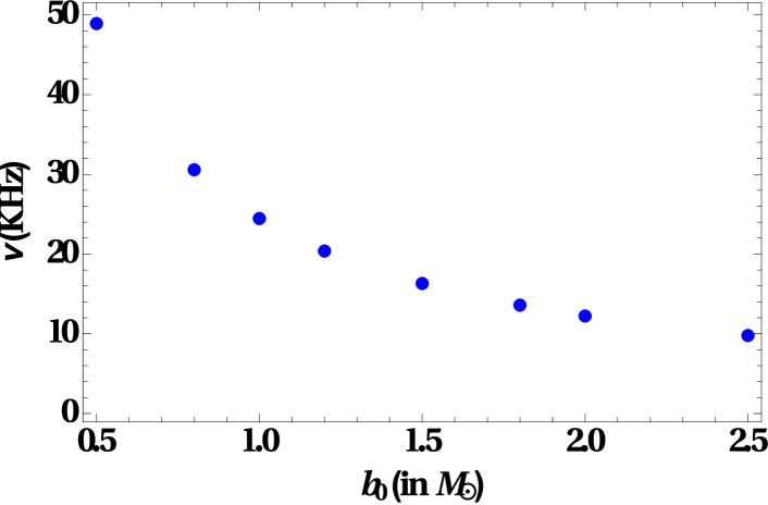
(a) Variation of frequency with throat radius.

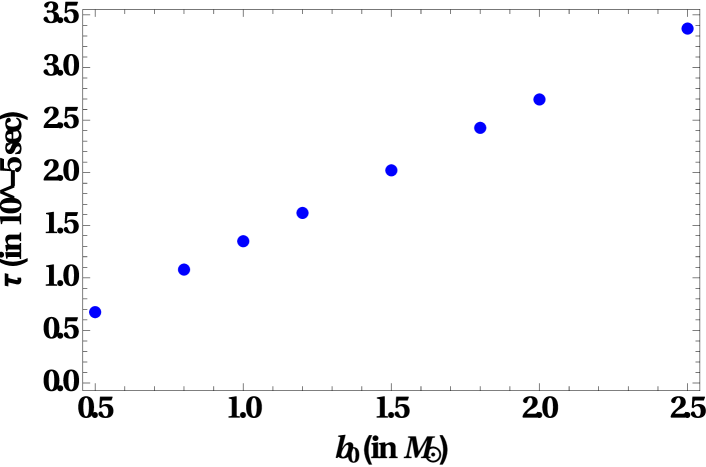
(b) Variation of damping time (scaled by a factor of $1/(2\pi)$) with throat radius.

Figure 6: QNMs corresponding to even state

We observe that as the throat radius increases, the frequency of the wave decreases and the damping time increases (Figure 6 (a, b)). This can be interpreted in the following way: if we assume that the wormhole is produced as a result of the merger of two compact bodies (merger of exotic compact objects has been studied in cardoso1 , krishnendu ) then, as the throat radius of the remnant wormhole increases, the frequency of the emitted wave decreases. As and when LIGO sensitivity is enhanced it may be possible to detect QNM signals, in future detections, from macroscopic wormholes with large throat radius Ligo , enhanced ligo .

V.4 Approximating known potentials with triangular barriers

Most of the perturbation potentials that arise in astrophysical scenarios are complicated and cannot be solved analytically. They can be solved only using numerical techniques. In order to get better analytic insight on characteristic features such as QNMs, the perturbation potentials may be approximated by known exactly solvable potentials like the rectangular barrier rectangular barrier , step barrier or the Poschl- Teller ferrari . In a similar way, since the triangular barrier is also an exactly solvable model, it may be used to approximate other potentials with which it has a resemblance in profile (barrier features). Perturbation potentials for wormholes are usually of the single or double barrier types. A prominent example is the Ellis–Bronnikov spacetime ellis . In the approach just mentioned, we can find the scalar QNMs of the Ellis–Bronnikov wormhole kim ; konoplya1 ; kunz by approximating it with a triangular barrier.
The line element and the effective potential for massless, scalar wave propagation in the Ellis–Bronnikov geometry are given by,

$$\mathrm{ds^{2}=-dt^{2}+\frac{dr^{2}}{1-\frac{b_{0}^{2}}{r^{2}}}+r^{2}(d\theta^{2}+sin^{2}\theta d\phi^{2})}$$ (60)

$$\mathrm{V_{eff}=\frac{\ell(\ell+1)}{(r_{*}^{2}+b_{0}^{2})}+\frac{b_{0}^{2}}{(r_{*}^{2}+b_{0}^{2})^{2}}}$$ (61)

with $\ell$ being related to angular momentum, $r^{2}=r_{*}^{2}+b_{0}^{2}$, where ‘r’ is the radial coordinate, ‘$r_{*}$’ is the tortoise coordinate and $b_{0}$ is the throat radius of the wormhole. In order to approximate the Ellis–Bronnikov perturbation potential with the triangular barrier we need to define the parameters $a$ and $V_{0}$ (for the triangular barrier) appropriately. The $V_{0}$ is set equal to the peak of the Ellis–Bronnikov perturbation potential at $r_{*}=0$ and the value of $a$ is set equal to the full width at half maximum of the curve representing the Ellis–Bronnikov potential (see Figure 7). A similar matching technique for a rectangular potential can be found in the appendix of kerr WH . The spatial coordinate $`x$’ in the case of triangular barrier acts as the tortoise coordinate and is similar to $r_{*}$. The following table (Table V) shows the fundamental QNM (least damped) frequencies obtained both by a numerical technique and by the approximation with the triangular barrier. It also mentions the values of $V_{0}$ and $a$ used in the calculations. The value of throat radius is taken as unity.

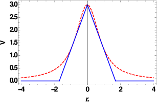
Figure 7: Fitting the Ellis-Bronnikov scalar perturbation potential (dashed line) with the triangular barrier (blue line) for $\ell=1$ mode.

To find the numerical results we have used the direct integration approach of Chandrasekhar and Detweiler Chandrasekhar . The differential equation (27) is directly integrated with the proper boundary conditions to obtain the QNMs paolo . For Ellis–Bronnikov geometry, the potential is symmetric about $r_{*}=0$ so the solutions can be divided into symmetric and anti-symmetric types. A similar treatment can be found in aneesh . Hence the initial conditions for the two classes of QNMs will be: $\psi(0)=0$ for antisymmetric solutions and $\psi^{\prime}(0)=0$ for symmetric solutions. We will only consider the symmetric case which has smaller damping. We have followed the procedure for direct integration as given in aneesh . The wave function is suitably expanded upto finite but arbitrary orders both near the throat and at spatial infinity. It is then substituted in the differential equation and evolved from both the throat and spatial infinity towards an in-between arbitrary point. Matching the wave function and its derivatives gives the QNMs.

$\ell$	$V_{0}$	$a$	$\omega$ (numerical)	$\omega$ (approximation)
1	3	1.69795	1.57234 -i 0.529818	1.68343 -i 0.435517
2	7	1.86257	2.54627 -i 0.512869	2.44744 -i 0.350497
3	13	1.92461	3.53387 -i 0.507184	3.22302 -i 0.462328
4	21	1.95296	4.5266 -i 0.504649	4.42191 -i 0.436661
5	31	1.96801	5.52182 -i 0.503319	5.23639 -i 0.43561
6	43	1.97688	6.51846 -i 0.502545	6.45926 -i 0.554812
7	57	1.98253	7.51595 -i 0.502061	7.26488 -i 0.463475
8	73	1.98635	8.51401 -i 0.501743	8.05989 -i 0.537328
9	91	1.98904	9.51247 -i 0.501526	9.309 -i 0.517387
10	111	1.99101	10.5112 -i 0.501373	10.1153 -i 0.517864

Table 5: Values of QNM frequencies for the Ellis-Bronnikov wormhole obtained by approximating with a triangular barrier.

It can be seen from Table V that the values obtained using the triangular barrier approximation are quite close to the values obtained by the above-stated numerical method. Thus, the triangular barrier can indeed be used to approximate similar smooth potentials which may arise as perturbation potentials in different spacetimes.

VI SUMMARY AND DISCUSSION

Let us now briefly summarise our results. A primary goal of our work as reported in this article was to find the scalar quasi-normal modes of a finite, symmetric triangular barrier potential. This problem, though exotic, has not been dealt with before in the literature. The solutions involve the Airy functions and the QNMs are hidden in a transcendental equation involving the Airy functions and their derivatives. A correspondence known due to early work by Ferrari and Mashhoon may be used to find the transcendental equation for the QNMs from those in the bound state problem (triangular well). We first find the condition for bound states (and the bound state energies and wave-functions) of the triangular well and use it to find the QNMs using a transformation. It is useful to note that one can also find the QNMs completely independently, without referring to the bound state problem at all. The complete time domain profiles are then obtained by numerically integrating the scalar wave equation. We extract the QNMs from the time domain profiles and compare with the analytically obtained values. The agreement is quite good.

Further, to provide a context for the triangular barrier, we have constructed a ‘sandwich’ wormhole geometry whose effective potential under scalar wave propagation will be a finite, symmetric triangular barrier, for the $m=0$ mode. The wormhole, thus constructed, has matter, with negative energy density, sandwiched over a finite region between two flat spacetimes. We find the QNMs for this geometry and also show, through the time-domain profiles, that this wormhole has a decaying late-time tail following the quasi-normal ringdown and is thus stable.

Since wormholes necessarily have perturbation potentials which are single or double barriers, we try to approximate one such case using the triangular barrier. We take the scalar perturbations of the Ellis-Bronnikov wormhole and model the barrier potential with a properly parametrised triangular barrier. A comparison of the QNMs for the smooth potential with those for the triangular barrier seems to be reasonably good.

In most realistic cases in gravitational wave or black hole physics the effective potentials are far more complicated. In order to find QNMs for such scenarios, numerical approaches are extensively employed. There are various numerical techniques available for finding QNMs. These include the direct integration method Chandrasekhar ,paolo due to Chandrasekhar-Detweiler, the Prony fit method ( a frequency extraction technique based on the fact that the time domain profile is dominated, in most cases, by the fundamental QNM ) konoplya ,prony1 , prony2 , prony3 , the continued fraction method by Leaver CF , to list a few. Generically, many of these potentials are barrier type (particularly those for wormholes) and may be modeled using rectangular rectangular barrier or triangular barriers, in appropriate limits. Further, double triangular barriers (similar to the double rectangular ones) may be used to model the interesting phenomenon of echoes which has generated quite some interest and activity in recent times kerr WH .

VII CONCLUSION

In conclusion, we have succeeded in adding a new exactly solvable problem to the list of analytic results (for QNMs) mentioned in visser . We have also shown that the triangular barrier can arise (i) as a scalar perturbation potential for a specially constructed wormhole geometry or (ii) as an approximation to the scalar perturbation potential in the Ellis-Bronnikov wormhole spacetime. In principle, our results may be used to model any scenario (gravitational or otherwise) where we have a symmetric, single barrier potential in a wave equation.

References

- (1) H. Lamb, On a Peculiarity of the wave‐system due to the free vibrations of a nucleus in an extended medium, Proc. Lond. Math. Soc.,s1-32 (1) (1900), pp. 208-213, .
- (2) T. Regge and J. A. Wheeler, Stability of a Schwarzschild singularity, Phys. Rev. 108, 1063 (1957).
- (3) F. J. Zerilli, Effective potential for even-parity Regge-Wheeler gravitational perturbation equations, Phys. Rev. Lett. 24, 737 (1970).
- (4) C. V. Vishveshwara, Scattering of gravitational radiation by a Schwarzschild black hole, Nature 227, 936 (1970).
- (5) C. V. Vishveshwara, Stability of the Schwarzschild metric, Phys. Rev. D 1, 2870 (1970).
- (6) S. Chandrasekhar and S. Detweiler, The quasi-normal modes of the Schwarzschild black hole, Proc. R. Soc. Lond. A 344,441 (1975).
- (7) G. Pöschl and E. Teller, Bemerkungen zur Quantenmechanik des anharmonischen Oszillators, Z. Physik 83, 143 (1933).
- (8) A. F. Cardona and C. Molina,Quasinormal modes of generalized Pöschl-Teller potentials, Class. Quant. Grav. 34 245002 (2017).
- (9) P. Boonserm and M. Visser, Quasi-normal frequencies: key analytic results, arXiv:1005.4483v3 [math-ph], JHEP, 1103:073 (2011).
- (10) B. P. Abbott et. al, Observation of gravitational waves from a binary black hole merger, Phys. Rev. Letts. 116, 061102 (2016).
- (11) S. Aneesh, S. Bose and S. Kar, Gravitational waves from quasinormal modes of a class of Lorentzian wormholes, Phys. Rev. D 97, 124004 (2018).
- (12) S. Bhattacharyya and S. Shankaranarayanan, Quasinormal modes as a distinguisher between general relativity and f(R) gravity: charged black holes, arXiv:1803.07576v3 [gr-qc] (2018).
- (13) B. F. Schutz and C. M. Will, Black hole normal modes - a semi-analytic approach, Astrophys. J., L291, 33 (1985).
- (14) A. K. Ghatak, E. G. Sauter and I. C. Goyal, Validity of the JWKB formula for a triangular potential barrier , Eur. Jr. Phys., Vol.18, 199 (1997).
- (15) B. Mashhoon, Quasi-normal modes of a black hole, Proceedings of the third Marcel Grossmann meeting on General Relativity, edited by H. Ning (1983) pp. 599–608.
- (16) V. Ferrari and B. Mashhoon, Oscillations of a black hole, Phys. Rev. Lett. 52, 1361 (1984).
- (17) V. Ferrari and B. Mashhoon, New approach to the quasinormal modes of a black hole, Phys. Rev. D 30, 295 (1984).
- (18) H.J. Blome and B. Mashhoon, Quasi-normal oscillations of a Schwarzschild black hole, Phys. Lett. A, Vol.100 , 231 (1984).
- (19) M. Morris and K. S. Thorne, Wormholes in spacetime and their use for interstellar travel: A tool for teaching general relativity, Am. J. Phys., 56, 395 (1988).
- (20) H. J. Ellis, Ether flow through a drainhole: a particle model in general relativity, J. Math. Phys. 14, 104 (1973); K. A. Bronnikov, Scalar tensor theory and scalar charge, Acta Phys. Polon. B4, 250 (1973)
- (21) V.Cardoso, Quasinormal modes and gravitational radiation in black hole spacetimes, arXiv:0404093v1 [gr-qc], Section: 1.1.2 (2004).
- (22) Digital Library of Mathematical Functions: Section 9.2 (v); https://dlmf.nist.gov/9.2.
- (23) Wolfram Research, Inc., Mathematica, Version 10.0, Champaign, IL (2014).
- (24) C. Gundlach, R. Price and J. Pullin, Late-time behavior of stellar collapse and explosions.I. Linearized perturbations, Phys. Rev. D 49 ,883 (1994).
- (25) R.A. Konoplya and A. Zhidenko, Quasinormal modes of black holes: from astrophysics to string theory, Rev. Mod. Phys. 83, 793 (2011).
- (26) H. P. Nollert, About the significance of quasi-normal Modes of Black Holes, Phys. Rev. D 53, 4397-4402 (1996).
- (27) V. Cardoso, S. Hopper, C. F. B. Macedo, C. Palenzuela and Paolo Pani, Echoes of ECOs: gravitational-wave signatures of exotic compact objects and of quantum corrections at the horizon scale, Phys. Rev. D 94, 084031 (2016).
- (28) N. V. Krishnendu, K. G. Arun, C. K. Mishra, Testing the binary black hole nature of a compact binary coalescence, Phys. Rev. Lett. 119, 091101 (2017).
- (29) D. V. Martynov, E. D. Hall, B. P. Abbott et. al., The sensitivity of the Advanced LIGO detectors at the beginning of gravitational wave astronomy, arXiv:1604.00439v3 [astro-ph.IM] (2016).
- (30) M. Page, J. Quin, J. L. Fontaine, C. Zhao, L. Ju and D. Blair, Enhanced detection of high frequency gravitational waves using optically diluted optomechanical filters, arXiv:1711.04469v2 [astro-ph.IM] (2017).
- (31) F. A. Handler and R. A. Matzner, Gravitational wave scattering, Phys. Rev. D 10, Vol. 22 (1980).
- (32) S. Kim, Wormhole perturbation and its quasi-normal modes, Prog. Theo. Phys. Suppl., No. 172, 21 (2008).
- (33) R. A. Konoplya, A. Zhidenko, Wormholes versus black holes: quasinormal ringing at early and late times, JCAP 12, 043 (2016).
- (34) J. L. Blázquez-Salcedo, X. Y. Chew and J. Kunz, Scalar and axial quasinormal modes of massive static phantom wormholes, Phys. Rev. D 98, 044035 (2018).
- (35) P. Bueno, P. A. Cano, F. Goelen, T. Hertog and B. Vercnocke, Echoes of Kerr-like wormholes, Phys. Rev. D 97, 024040 (2018).
- (36) P. Pani, Advanced methods in black-hole perturbation theory, arXiv:1305.6759v2 [gr-qc] (2013).
- (37) L. London, J. Healy and D. Shoemaker, Modeling ringdown: beyond the fundamental quasinormal modes, Phys. Rev. D 90, 124032 (2014).
- (38) E. Berti, V. Cardoso, J. A. González and U. Sperhake, Mining information from binary black hole mergers: a comparison of estimation methods for complex exponentials in noise, Phys. Rev. D 75, 124017 (2007).
- (39) O. P. F. Piedra, Gravitino perturbations in Schwarzschild black holes, Int. J. Mod. Phys. D 20:93–109 (2011).
- (40) E.W. Leaver, An analytic representation for the quasi-normal modes of Kerr black Holes, Proc. R. Soc. Lond., A 402, 285 (1985).