Abstract

In many high-throughput experimental design settings, such as those common in biochemical engineering, batched queries are more cost effective than one-by-one sequential queries. Furthermore, it is often not possible to directly choose items to query. Instead, the experimenter specifies a set of constraints that generates a library of possible items, which are then selected stochastically. Motivated by these considerations, we investigate Batched Stochastic Bayesian Optimization (BSBO), a novel Bayesian optimization scheme for choosing the constraints in order to guide exploration towards items with greater utility. We focus on site-saturation mutagenesis, a prototypical setting of BSBO in biochemical engineering, and propose a natural objective function for this problem. Importantly, we show that our objective function can be efficiently decomposed as a difference of submodular functions (DS), which allows us to employ DS optimization tools to greedily identify sets of constraints that increase the likelihood of finding items with high utility. Our experimental results show that our algorithm outperforms common heuristics on both synthetic and two real protein datasets.

1 Introduction

Bayesian optimization is a popular technique for optimizing black-box objective functions, with applications in (sequential) experimental design, parameter tuning, recommender systems and more. In the classical setting, Bayesian optimization techniques assume that items can be directly queried at each iteration. However, in many real-world applications such as those in biochemical engineering, direct querying is not possible: instead, a (constrained) library of items is specified, and then batches of items from the library are stochastically queried.

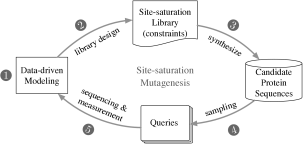
Figure 1: Data-driven site-saturation mutagenesis. (1) Machine learning model for predicting certain protein properties; (2) site-saturation library design; (3) synthesize protein sequences according to the site-saturation libraries; (4) randomly sample proteins for sequencing; (5) sequence and measure the properties of the sampled proteins.

As a prototypical example in biochemical engineering, let us consider site-saturation mutagenesis (SSM) (Voigt et al., 2001), a protein-engineering strategy that mutates a small number of critical sites in a protein sequence (cf. Fig. 1). At each round, a combinatorial library is designed by specifying which amino acids are allowed at the specified sites (step (1-3)), and then a batch of amino acid sequences from the library is sampled with replacement (step 4). The sampled sequences are evaluated for their ability to perform a desired function (step 5), such as a chemical reaction.

Ideally, at each iteration, the amino acids to be considered at each site should be chosen to maximize the number of improved sequences expected in the stochastic batch sample from the resulting library. Finding such libraries is highly non-trivial: it requires solving a combinatorial optimization problem over an exponential number of items. Libraries are designed by choosing the allowed amino acids at each site (‘constraints’) from the set of all amino acids at all sites. Adding allowed constraints results in an exponential number of items in the library. As mentioned above, these challenges are exacerbated due to the uncertainty from sampling batches of queries. Thus, new optimization schemes and algorithmic tools are needed for addressing such problems.

Our contribution

In this paper, we investigate Batched Stochastic Bayesian Optimization (BSBO), a novel Bayesian optimization scheme for choosing a library design in order to guide exploration towards items with greater utility. This scheme is unique in that we choose a library design instead of directly querying items, and the items are queried in stochastic batches (e.g. 10-1000 items per batch). In particular, we focus on library design for site-saturation mutagenesis, and identify a natural objective function that evaluates the quality of a library design given the current information about the system. We propose Online-DSOpt, an efficient online algorithm for optimization over stochastic batches. In a nutshell, Online-DSOpt assembles each batch by decomposing the objective function into the difference of two submodular functions (DS). This allows us to employ DS optimization tools (e.g., Narasimhan & Bilmes (2005)) to greedily identify sets of constraints that increase the likelihood of finding items with high utility. We demonstrate the performance of Online-DSOpt on both synthetic and two experimentally-generated protein datasets, and show that our algorithm in general outperforms conventional greedy heuristics and efficiently finds rare, highly-improved, sequences.

2 Related Work

Bayesian optimization with Gaussian processes

Our work addresses a specific setting for Gaussian process (GP) optimization. GPs are infinite collections of random variables such that every finite subset of random variables has a multivariate Gaussian distribution. A key advantage of GPs is that inference is very efficient, which makes them one of the most popular theoretical tools for Bayesian optimization (Rasmussen & Williams, 2006; Srinivas et al., 2010; Wang et al., 2016). Notably, Srinivas et al. (2010) introduce the Gaussian Process Upper Confidence Bound (GP-UCB) algorithm for Bayesian Bandit optimization, which provides bounds on the cumulative regret when sequentially querying items. Desautels et al. (2014) generalize this to batch queries. In contrast to our setting, these algorithms require the ability to directly query items, either sequentially or in batches.

GP optimization for protein engineering

GP-UCB has been used to find improved protein sequences when sequences can be queried directly (Romero et al., 2013; Bedbrook et al., 2017). GPs (Saito et al., 2018) and other machine-learning methods (Wu et al., 2019) have been used to select constraints for SSM libraries. However, previous work relied on ad-hoc heuristics and do not provide a general procedure for selecting constraints in a model-driven way.

Information-parallel learning

In addition to the bandit setting (Desautels et al., 2014), there is a large body of literature on various machine learning settings that exploit information-parallelism. For example, in large-scale optimization, mini-batch/parallel training has been extensively explored to reduce the training time of stochastic gradient descent (Li et al., 2014; Zinkevich et al., 2010). In batch-mode active learning (Hoi et al., 2006; Guillory & Bilmes, 2010; Chen & Krause, 2013), an active learner selects a set of examples to be labeled simultaneously. The motivation behind batch active learning is that in some cases it is more cost-effective to request labels in large batches, rather than one-at-a-time. This setting is also referred to as buy-in-bulk learning (Yang & Carbonell, 2013). In addition to the simpler modeling assumption of being able to directly issue queries, these approaches also differ from our setting in terms of the objective: the batch-mode active learning algorithms aim to find a set of items that are maximally informative about some target hypothesis (hence to maximally explore), whereas we want to identify the best item (i.e., to both explore and exploit).

Submodularity and DS optimization

Submodularity (Nemhauser et al., 1978) is a key tool for solving many discrete optimization problems, and has been widely recognized in recent years in theoretical computer science and machine learning. While a growing number of previously studied problems can be expressed as submodular minimization (Jegelka & Bilmes, 2011) or maximization (Kempe et al., 2003; Krause & Guestrin, 2007) problems, standard maximization and minimization formulations only capture a small subset of discrete optimization problems. Narasimhan & Bilmes (2005) show that any set function $q$ can be decomposed as the difference of two submodular functions $h$ and $g$. Replacing $h$ with its modular upper bound, $g$ with its modular lower bound, or both reduces the problem of minimizing $q$ to a series of submodular minimizations, submodular maximizations, or modular minimizations, respectively, that are guaranteed to reduce $q$ at every iteration and to arrive at a local minimum of $q$ (Iyer & Bilmes, 2012). In general, computing a DS decomposition requires exponential time. We present two polynomial-time decompositions of our objective function.

3 Problem Statement

3.1 Problem Setup

We aim to optimize a black box utility function, $f:{\mathcal{X}}\rightarrow\mathbb{R}$. In contrast to classical Bayesian optimization, which sequentially queries the function value $f(x_{t})$ for an selected item $x_{t}\in{\mathcal{X}}$, we assume that the experimenter can only choose a subset of constraints (i.e., rules for generating items) from a ground set ${\mathcal{C}}$, based on which a stochastic batch of items are generated and measured. More concretely, we consider the following interactive protocol, as illustrated in Fig. 2. At each round the following happens:

• The algorithm chooses a set of constraints ${\mathcal{S}}\subseteq{\mathcal{C}}$ based on current knowledge of $f$ (Fig. 2, step (2)).

• The chosen constraints are used to construct a library of candidate queries: $Q({\mathcal{S}})\subseteq{\mathcal{X}}$, where $Q:2^{\mathcal{C}}\rightarrow 2^{\mathcal{X}}$ denotes the physical process that produces items under these constraints (Fig. 2, step (3)).

• A batch of $n$ queries ${\mathcal{B}}_{Q}({\mathcal{S}},\phi)\subseteq{\mathcal{X}}$ is randomly selected from the library $Q({\mathcal{S}})$ via a stochastic sampling procedure (Fig. 2, step (4)). Here, $\phi$ represents the random state of the sampling procedure ${\mathcal{B}}_{Q}$.

• When querying each item $x\in{\mathcal{B}}_{Q}({\mathcal{S}},\phi)$, we observe the function value there, perturbed by noise: $y=f(x)+\varepsilon(x)$. Here, the noise $\varepsilon(x)\sim\mathcal{N}(0,\sigma^{2})$ represents i.i.d. Gaussian white noise. We further assume that querying each item $x$ achieves reward $f(x)$ and incurs some cost $c(\{x\})$, where $c:2^{\mathcal{X}}\rightarrow\mathbb{R}$ denotes the cost function of a set of items (Fig. 2, step (5)).

• The results of the queries are used to update $f$.

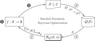
Figure 2: The batched stochastic Bayesian optimization setting. (1) Bayesian modeling (2) combinatorial constraints design; (3) candidate query generation; (4) random sampling; (5) batched queries.

We model $f$ as a sample from a Gaussian process, denoted by $f\sim\text{GP}\left({\mu(x),k(x,x^{\prime})}\right)$. Suppose that we have queried ${\mathcal{A}}\subseteq{\mathcal{X}}$ and received ${\mathbf{y}}_{\mathcal{A}}=[f(x_{i})+\varepsilon(x_{i})]_{x_{i}\in{\mathcal{A}}}$ observations. We can obtain the posterior mean $\mu_{\mathcal{A}}(x)$ and covariance $k_{\mathcal{A}}{(x,x^{\prime})}$ of the function through the covariance matrix $K_{\mathcal{A}}=[k(x_{i},x_{j})+\sigma^{2}\mathds{1}]_{x_{i},x_{j}\in{\mathcal{A}}}$ and ${\mathbf{k}}_{\mathcal{A}}(x)=[k(x_{i},x)]_{x_{i}\in{\mathcal{A}}}$:

$$\mu_{\mathcal{A}}(x) =\mu(x)+{\mathbf{k}}_{\mathcal{A}}(x)^{\intercal}K_{\mathcal{A}}^{-1}{\mathbf{y}}_{\mathcal{A}},$$

$$k_{\mathcal{A}}{(x,x^{\prime})} =k(x,x^{\prime})-{\mathbf{k}}_{\mathcal{A}}(x)^{\intercal}K_{\mathcal{A}}^{-1}{\mathbf{k}}_{\mathcal{A}}(x^{\prime}).$$

3.2 The Objective

Simple regret

Our overall goal is to minimize the (expected) simple regret, defined as $R_{t}(x)=f(x^{*})-f(x_{t})$ over $T$ rounds, where $x^{*}=\operatorname*{arg\,max}_{x\in{\mathcal{X}}}f(x)$ is the item of the maximum utility. In other words, we aim to maximize the reward in order to converge to performing as well as $x^{*}$ as efficiently as possible. We refer to this problem as the batched stochastic Bayesian optimization (BSBO) problem.

Acquisition function

Assume that we have a budget of querying $n$ items for each batch of experiments and that each batch ${\mathcal{B}}_{Q}$ is selected by sampling uniformly from the library. At each iteration, we wish to select the constraints ${\mathcal{S}}$ that will maximize the (expected) number of improved items observed in the next stochastic batched query. If the current best item has a value $\tau$, then we seek a set of constraints ${\mathcal{S}}^{*}\in\operatorname*{arg\,max}F({\mathcal{S}})$, where:

$$F({\mathcal{S}})=\mathbb{E}_{\phi}\!\left[\sum_{x\in{\mathcal{B}}_{Q}({\mathcal{S}})}\mathbbm{1}(f(x)>\tau)\right].$$ (3.1)

Here, $\mathbbm{1}$ is the indicator function. This objective is intractable under the GP posterior, as the dependencies between $f(x)$ preclude a closed form. We ignore the dependencies between the utilities to arrive at the following surrogate function;

$$\hat{F}({\mathcal{S}})=\sum_{x\in Q({\mathcal{S}})}\rho(x)\left[1-\left({1-\frac{1}{|Q({\mathcal{S}})|}}\right)^{n}\right].$$ (3.2)

The rewards $\rho(x)=P(f(x)>\tau)$ can be computed for all $x\in Q({\mathcal{C}})$ from the GP posterior for each item using the Gaussian survival function by ignoring off-diagonal entries in the predictive posterior covariance. Note that this surrogate acquisition function $\hat{F}$ captures the expected reward under an independence assumption. As we will demonstrate later in §LABEL:sec:exp:real, despite such an assumption, we observe a strong correlation between $\hat{F}$ and $F$ on the experimental datasets we study, which are known to have high dependencies between the rewards $\rho(x)$ of different items.

3.3 Site-Saturation Library Design

We now consider the site-saturation library design problem as a special case of BSBO. In site-saturation mutagenesis, the utility function $f(x)$ specifies the utility of a protein sequence $x$, and the constraint set ${\mathcal{C}}=\bigcup_{\ell=1}^{L}{\mathcal{C}}^{\left({\ell}\right)}$ specifies the set of amino acids allowed at each site of the protein sequence. $L$ denotes the number of sites, and ${\mathcal{C}}^{\left({\ell}\right)}$ denotes the set of all possible amino acids at site $\ell$. We denote the set of amino acids selected for site $\ell$ by ${\mathcal{S}}^{\left({\ell}\right)}$; hence ${\mathcal{S}}=\bigcup_{\ell=1}^{L}{\mathcal{S}}^{\left({\ell}\right)}$. The candidate query pool (library) $Q$ consists of all possible protein sequences that can be generated w.r.t. the constraints: ${\mathcal{S}}$:

$$Q\left({{\mathcal{S}}}\right)=\prod_{\ell=1}^{L}{\mathcal{S}}^{\left({\ell}\right)}.$$ (3.3)

Note that adding constraints generally increases the number of allowed items.

1 Input: Constraints set ${\mathcal{C}}=\bigcup_{\ell=1}^{L}{\mathcal{C}}^{\left({\ell}\right)}$; number of rounds $T$; budget on each batch $n$; GP prior on $f$

begin

      2 ${\mathcal{A}}\leftarrow\emptyset$

       /* iteratively select the next batch */

       for $t$ in ${1,\dots,T}$ do

             /* compute the reward matrix $M=\{f(x)\}$ */

            3 $M\leftarrow\textsf{ComputeReward}(\text{posterior on~{}}f,{\mathcal{A}})$

            4 ${\mathcal{S}}\leftarrow\textsf{DSOpt}({\mathcal{C}},M,n)$

             /* posterior update */

            5 ${\mathcal{A}}\leftarrow{\mathcal{A}}\cup{\mathcal{B}}_{Q}({\mathcal{S}},\phi)$

      6Output: Optimizer of $f$

      

Algorithm 1 Online Batched Constraints Design via DS Optimization (Online-DSOpt)

4 Algorithms

1 Input: Constraints set ${\mathcal{C}}=\bigcup_{\ell=1}^{L}{\mathcal{C}}^{\left({\ell}\right)}$; reward matrix $M=\{f(x)\}$; budget on each batch $n$

begin

      2 Set up $\hat{F}$ from the inputs $(M,n)$

       /* Decompose $\hat{F}$ into diff of submod funcs. */

      3 $h,g\leftarrow\textsf{DSConstruct-SA}(\hat{F},{\mathcal{C}})$

       (or $h,g\leftarrow\textsf{DSConstruct-DC}(\hat{F},{\mathcal{C}})$)

       /* Initiliaze the starting position */

      4 ${\mathcal{S}}_{\text{cand}}\leftarrow\emptyset$

      5 ${\mathcal{S}}\leftarrow\textsf{Init}({\mathcal{C}})$

       /* Optimize $h-g$ using ModMod or SupSub. */

       while ${\mathcal{S}}$ not converged do

             /* Keep track of local search solutions */

            6 ${\mathcal{S}}_{\text{cand}}\leftarrow{\mathcal{S}}_{\text{cand}}\cup\textsf{LocalSearch}(\hat{F},{\mathcal{S}},{\mathcal{C}})$

             /* Make a greedy move from ${\mathcal{S}}$ */

            7 ${\mathcal{S}}\leftarrow\textsf{ModMod}(h-g,{\mathcal{S}},{\mathcal{C}})$

             (or ${\mathcal{S}}\leftarrow\textsf{SupSub}(h-g,{\mathcal{S}},{\mathcal{C}})$)

            

      8${\mathcal{S}}_{\text{cand}}\leftarrow{\mathcal{S}}_{\text{cand}}\cup\{{\mathcal{S}}\}$

       /* pick the best among candidate solutions */

      9 ${\mathcal{S}}^{*}\leftarrow\operatorname*{arg\,min}_{{\mathcal{S}}\in{\mathcal{S}}_{\text{cand}}}{\left\{\hat{F}({\mathcal{S}})\right\}}$

      10 Output: Set of selected constraints ${\mathcal{S}}^{*}$

      

Algorithm 2 DS Optimization (DSOpt)

We now present Online-DSOpt (Algorithm 1), an online learning framework for (online) batched stochastic Bayesian optimization. Our framework relies on a novel discrete optimization subroutine, DSOpt, which aims to maximize the expected reward for each batched experiment. At each iteration, Online-DSOpt uses a GP trained on previously-observed items to compute the reward for each item $x\in Q({\mathcal{C}})$ (cf., Line 1) and then invokes DSOpt to select constraints. Pseudocode for DSOpt is presented in Algorithm 2. A batch of items is then sampled stochastically from the resulting library and used to update the GP.

A key component of the DS optimization subroutine DSOpt is a DS decomposition of the objective. Note that in general, finding a DS decomposition of an arbitrary set function requires searching through a combinatorial space and can be computationally prohibitive. As one of our main contributions, we present two polynomial time algorithms, DSConstruct-SA (Algorithm 3) and DSConstruct-DC (Algorithm 4), for decomposing our surrogate objective. Both algorithms exploit the structure of the objective function: DSConstruct-SA decomposes the objective via submodular augmentation (Narasimhan & Bilmes, 2005); DSConstruct-DC decomposes the objective via a difference of convex functions (DC) decomposition.

4.1 DS Optimization

After obtaining the submodular decomposition $\hat{F}=-(h-g)$, DSOpt (Algorithm 2) proceeds to greedily optimize the DS function. For example, let us consider running the Modular-modular procedure (ModMod) (Iyer & Bilmes, 2012) for making a greedy move at Line 2 of Algorithm 2. Since our goal is to maximize $-(h-g)$ (i.e., to minimize $h-g$), we will seek to minimize the upper bound on $h-g$. The ModMod procedure constructs a modular upper bound on the first submodular component, denoted by $\textsf{ub}^{h}\geq h$, and a modular lower bound on the second submodular component, denoted by $\textsf{lb}^{g}\leq g$. Both modular bounds are tight at the current solution ${\mathcal{S}}$: $\textsf{ub}^{h}({\mathcal{S}})=h({\mathcal{S}})$, $\textsf{lb}^{g}({\mathcal{S}})=g({\mathcal{S}})$. ModMod then tries to solve the following optimization problem, starting from ${\mathcal{S}}$:

$${\mathcal{S}}^{*}\in\operatorname*{arg\,min}_{{\mathcal{S}}}\left({\textsf{ub}^{h}({\mathcal{S}})-\textsf{lb}^{g}({\mathcal{S}})}\right).$$

To ensure that we find a better solution, we augment the ModMod procedure with a sequence of additional local search solutions, and in the end pick the best among all. The local search procedure, LocalSearch (cf. Line 2 of Algorithm 2), sequentially makes greedy steps (by adding or removing a constraint from the current solution) until no further action is improving the current solution. The following theorem states that our DS optimization subroutine DSOpt is guaranteed to find a “good” solution:

Theorem 1 (Adapted from Iyer & Bilmes (2012)).

Algorithm 2 is guaranteed to find a set of constraints that achieves a local maximum of $\hat{F}$.

1 Input: Constraints set ${\mathcal{C}}=\bigcup_{\ell=1}^{L}{\mathcal{C}}^{\left({\ell}\right)}$; surrogate objective function $\hat{F}$, budget on each batch $n$; selected constraints ${\mathcal{S}}$

begin

      2 $v(x)\leftarrow\sqrt{x}$ for $x\in\{1,\dots,|{\mathcal{C}}|\}$

      3 $\alpha\leftarrow v(n-2)+v(n)-2v(n-1)$

       /* compute $\beta^{\prime}$ of Eq.(4.2) */

       foreach $x\in\{1,\dots,|Q({\mathcal{C}})|\}$ do

            4 $r_{1}(x)\leftarrow\left({1-\frac{1}{s}}\right)^{n}-\left({1-\frac{1}{2s}}\right)^{n}$

            5 $r_{2}(x)\leftarrow\max_{\mathcal{T}:|\mathcal{T}|\leq s}\sum_{x\in\mathcal{T}}f(x)$

      6$\beta^{\prime}\leftarrow-\max_{x}{r_{1}(x)r_{2}(x)}$

      7 $h_{1}({\mathcal{S}})\leftarrow\frac{|\beta^{\prime}|}{\alpha}v(|{\mathcal{S}}|)$

      8 $g_{1}({\mathcal{S}})\leftarrow\hat{F}({\mathcal{S}})+\frac{|\beta^{\prime}|}{\alpha}v(|{\mathcal{S}}|)$

      9 Output: DS decomposition $\hat{F}=-(h_{1}-g_{1})$

      

Algorithm 3 DS Construction via Submodular Augmentation (DSConstruct-SA)

4.2 DS Construction via Submodular Augmentation

It is well-established that every set function can be expressed as the sum of a submodular and a supermodular function (Narasimhan & Bilmes, 2005). In particular, Iyer & Bilmes (2012) provide the following constructive procedure for decomposing a set function into the DS form: Given a set function $q$, one can define $\beta=\min_{{\mathcal{S}}\subseteq{\mathcal{S}}^{\prime}\subseteq{\mathcal{C}}\setminus j}\Delta_{q}(j\mid{\mathcal{S}})-\Delta_{q}(j\mid{\mathcal{S}}^{\prime})$, where $\Delta_{q}(j\mid{\mathcal{S}}):=q({\mathcal{S}}\cup\{j\})-q({\mathcal{S}})$ denotes the gain of adding $j$ to ${\mathcal{S}}$. When $q$ is not submodular, we know that $\beta<0$. Now consider any strictly submodular function $p$, with $\alpha=\min_{{\mathcal{S}}\subseteq{\mathcal{S}}^{\prime}\subseteq{\mathcal{C}}\setminus j}\Delta_{p}(j\mid{\mathcal{S}})-\Delta_{p}(j\mid{\mathcal{S}}^{\prime})>0$. Define $h({\mathcal{S}})=q({\mathcal{S}})+\frac{|\beta^{\prime}|}{\alpha}p({\mathcal{S}})$ for any $\beta^{\prime}<\beta$. It is easy to verify that $h$ is submodular since $\min_{{\mathcal{S}}\subseteq{\mathcal{S}}^{\prime}\subseteq{\mathcal{C}}\setminus j}\Delta_{h}(j\mid{\mathcal{S}})-\Delta_{h}(j\mid{\mathcal{S}}^{\prime})\geq\beta+|\beta^{\prime}|\geq 0$. Hence $q({\mathcal{S}})=h({\mathcal{S}})-\frac{|\beta|}{\alpha}p({\mathcal{S}})$ is a difference between two submodular functions.

We refer to the above decomposition strategy as DSConstruct-SA (where SA stands for “submodular augmentation”), and present the pseudo code in Algorithm 3. As suggested in (Iyer & Bilmes, 2012), we choose the submodular augmentation function $p({\mathcal{S}})=v(|{\mathcal{S}}|)$, where $v(x)$ is a concave function, and therefore $\alpha=\min_{x\leq x^{\prime};x,x^{\prime}\subseteq\mathbb{Z}}v(x+1)-v(x)-v(x^{\prime}+1)-v(x^{\prime})$. This leads to the following decomposition of our surrogate objective $\hat{F}$:

$$\hat{F}({\mathcal{S}})=\underbrace{\left({\hat{F}({\mathcal{S}})+\frac{|\beta^{\prime}|}{\alpha}v(|{\mathcal{S}}|)}\right)}_{g_{1}({\mathcal{S}})}-\underbrace{\frac{|\beta^{\prime}|}{\alpha}v(|{\mathcal{S}}|)}_{h_{1}({\mathcal{S}})},$$ (4.1)

where $h_{1}$, $g_{1}$ by construction are submodular functions, and $\beta^{\prime}$ is a lower bound on $\beta$:

$$\beta^{\prime}\leq\beta=\min_{{\mathcal{S}}\subseteq{\mathcal{S}}^{\prime}\subseteq{\mathcal{C}}\setminus j}\Delta_{\hat{F}}(j\mid{\mathcal{S}})-\Delta_{\hat{F}}(j\mid{\mathcal{S}}^{\prime}).$$ (4.2)

The key step of the DSConstruct-SA algorithm is to construct such a lower bound $\beta^{\prime}$. The following lemma, which is proved in the Appendix, shows that one can compute $\beta^{\prime}$ in polynomial time, and hence can efficiently express $\hat{F}$ as a DS as defined in Eq. (4.1).

Lemma 2.

Algorithm 3 returns a DS-decomposition of $\hat{F}$ in polynomial time.

1 Input: Constraints set $\prod_{\ell=1}^{L}{\mathcal{C}}_{\ell}$; budget on each batch $n$; selected constraints ${\mathcal{S}}$

begin

      2 $u(x)\leftarrow\frac{x^{2}}{2}$, $\alpha\leftarrow 1$

      3 $r(x)\leftarrow\left({1-\frac{1}{x}}\right)^{n}$,

      4 $\beta\leftarrow\left|\min_{x}r^{\prime\prime}(x)\right|$ for $x\in\{1,\dots,|Q({\mathcal{C}})|\}$.

      5 $h_{2}({\mathcal{S}})\leftarrow-\left({1+\frac{\beta}{\alpha}u(Q(|{\mathcal{S}}|))}\right){\sum_{x\in Q({\mathcal{S}})}{f(x)}}$

      6 $g_{2}({\mathcal{S}})\leftarrow-\left({r(|Q({\mathcal{S}})|)+\frac{\beta}{\alpha}u(Q(|{\mathcal{S}}|))}\right)\sum_{x\in Q({\mathcal{S}})}{f(x)}$

      7 Output: DS decomposition $\hat{F}=-(h_{2}-g_{2})$

      

Algorithm 4 DS Construction via DC Decomposition (DSConstruct-DC)

4.3 DS Construction via DC Decomposition

We now consider an alternative strategy for decomposing the surrogate function $\hat{F}$, based on a novel construction procedure that reduces to expressing a continuous function as the difference of convex (DC) functions. Concretely, we note that $\hat{F}({\mathcal{S}})$ consists of two (multiplicative) terms: (i) a supermodular set function $\sum_{x\in Q({\mathcal{S}})}f(x)$, and (ii) a set function that only depends on the cardinality of the input, i.e., $\sum_{x\in Q({\mathcal{S}})}f(x)\left({1-\left({1-\frac{1}{|Q({\mathcal{S}})|}}\right)^{n}}\right)$. As is further discussed in the Appendix, we show that one can exploit this structure, and focus on the DC decomposition of term (ii). We provide the detailed algorithm in Algorithm 4, and refer to it as DSConstruct-DC (where DC stands for “difference of convex decomposition”).

It is easy to check from Algorithm 3 that DSConstruct-SA runs in quadratic time w.r.t. $|Q({\mathcal{C}})|$. In contrast, DSConstruct-DC only requires finding the minimum of an array of size $|Q({\mathcal{C}})|$, which, in the best case, runs in linear time w.r.t. $|Q({\mathcal{C}})|$. At the end of the algorithm, DSConstruct-DC outputs the following DS function:

$$\hat{F}({\mathcal{S}}) =\underbrace{\sum_{x\in Q({\mathcal{S}})}\left({-\rho(x)}\right)\cdot\left({r(|Q({\mathcal{S}})|)+\frac{\beta}{\alpha}u(Q(|{\mathcal{S}}|))}\right)}_{g_{2}({\mathcal{S}})}$$

$$\quad-\underbrace{{\sum_{x\in Q({\mathcal{S}})}\left({-\rho(x)}\right)\left({1+\frac{\beta}{\alpha}u(Q(|{\mathcal{S}}|))}\right)}}_{h_{2}({\mathcal{S}})}.$$ (4.3)

where $u(x)$ is a non-negative, monotone convex function, $\alpha=\min_{x}u^{\prime\prime}(x)$, $r(x)=\left({1-\frac{1}{x}}\right)^{n}$, and $\beta=\left|\min_{x}r^{\prime\prime}(x)\right|$. We then prove the following results:

Lemma 3.

With the decomposition as defined in Eq. (4.3), both functions $h$, $g$ are submodular and hence we obtain a DS-decomposition of $\hat{F}$.

5 Experiments

In this section, we empirically evaluate our algorithm on three datasets. We first describe the datasets, then we provide empirical justification for our surrogate objective. Finally we provide quantitative evaluation of our algorithm against a few simple greedy heuristics.

5.1 Datasets

We test our algorithms on two experimental protein-engineering datasets and a synthetic dataset designed to have multiple local minima. The synthetic dataset has two sites with ${\mathcal{C}}^{\left({1}\right)}={\mathcal{C}}^{\left({2}\right)}=26$. Values for the items in the library are constructed such that there are disjoint blocks of items with non-zero $\rho(x)$ separated by regions where $\rho(x)=0$. This guarantees that there are multiple local optima in the constraint space. The experimental datasets consist of measured fitness values for every sequence in four-site SSM libraries for protein G domain B1 (GB1) (Wu et al., 2016), an immunoglobulin binding protein, and the protein kinase PhoQ (Podgornaia & Laub, 2015). These fitness landscapes are known to have high levels of multi-site epistasis. Having measurements for every fitness value in each library allows us to simulate engineering via multiple rounds of SSM.

5.2 Suitability of the surrogate objective

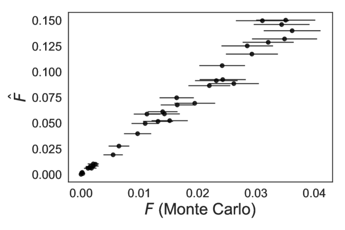
(a) $\hat{F}$ vs. $F$ for GB1

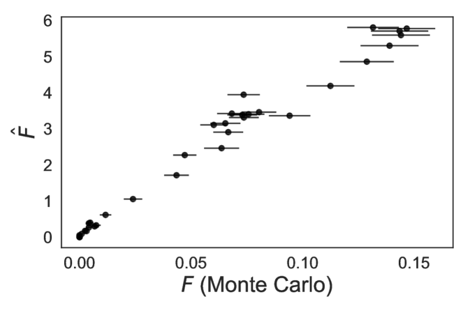
(b) $\hat{F}$ vs. $F$ for PhoQ

Figure S2: Comparing $\hat{F}$ (Eq. (3.2)) against the Monte Carlo estimates of $F$ (Eq. (3.1)). Error bars are standard errors for the Monte Carlo estimates. The approximate objective correlates well with Monte Carlo estimates of the exact objective.

Online-DSOpt uses a GP posterior to model the unobserved utilities. However, there is no closed form for the true batch constraint design objective, which is to choose constraints ${\mathcal{S}}$ that maximize the expected number of improved observations found by querying $Q({\mathcal{S}})$. The approximate objective function (Equation 3.2) ignores dependencies between items, and thus will overestimate the true objective. To test the suitability of the approximate objective function, we selected an initial batch of sequences from the PhoQ dataset consisting of all the single mutants plus 100 randomly-selected sequences, trained a GP regression model, and used the posterior to compute the rewards $\rho(x)$. Figure S2 shows that values for the approximate objective are well-correlated with the true objective estimated using Monte Carlo sampling. However, the independence assumption leads to overestimating the number of improved sequences that will be found.

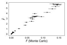
Figure 3: Comparing the full objective function approximated using Monte Carlo sampling and approximated with an independence assumption, as in Equation 3.2. Error bars are standard errors for the Monte Carlo estimates.

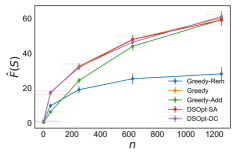
Figure 4: Performance of each algorithm on finding constraints for the synthetic dataset. Error bars are standard errors.

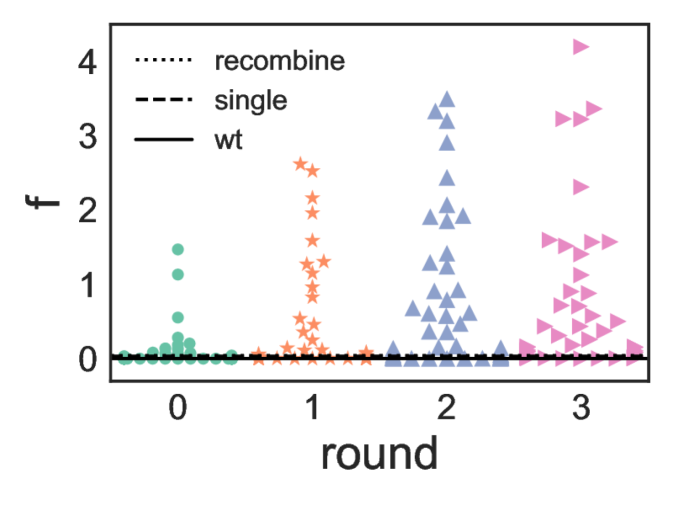
(a) Simulation for GB1

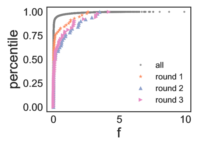
(b) e-CDFs for GB1

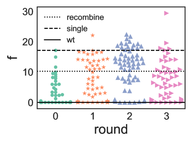
(c) Simulation for PhoQ

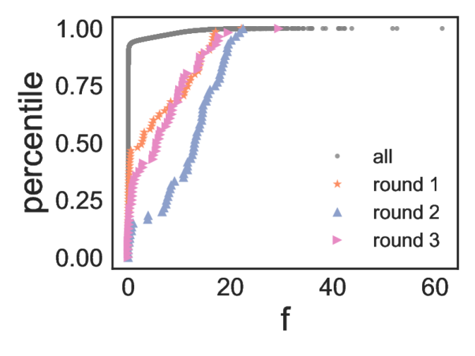
(d) e-CDFs for PhoQ

Figure 5: Experimental results. (a) and (c) show fitness values for the sequences sampled at each round for GB1 and PhoQ, respectively. The solid horizontal lines show the fitnesses for the wild-type sequences (wt). The dashed horizontal lines show the fitnesses for the best sequences with exactly one mutation from the wild type (single). The dotted horizontal lines show the fitnessees for the sequences that combine the best amino acid at each site determined in the wild-type background. (b) and (d) show empirical cumulative distribution functions (e-CDFs) for the entire library and for each sequence selected using Online-DSOpt in rounds 1 - 3 for GB1 and PhoQ, respectively.

5.3 Algorithm comparisons

Next, we compare the performance of Online-DSOpt using DSOpt-SA and DSOpt-DC against three greedy variants using the synthetic dataset. Greedy-Add greedily adds constraints, Greedy-Rem greedily removes constraints, and Greedy greedily adds or removes constraints until the objective stops improving. Because the empty set is a local optimum (adding any single constraint still results in no valid queries), it is necessary to begin the optimization at a set of constraints that yields a non-empty set of queries.

We compare the algorithms at a range of batchsizes $n$. At each $n$, we initialize each algorithm at ${\mathcal{C}}$, the constraints that result in the single best query, and 18 randomly selected sets of constraints. Figure 4 shows that DSOpt-SA, DSOpt-DC, and Greedy strongly outperform Greedy-Add and Greedy-Rem across all values of $n$. At small $n$, the optima tend to have few constraints, so Greedy-Add performs particularly poorly. As $n$ approaches infinity, the optimum approaches the ground set ${\mathcal{C}}$, and so Greedy-Rem performs particularly poorly. DSOpt-SA, DSOpt-DC, and Greedy perform very similarly across all values of $n$. In theory, DSOpt-SA and DSOpt-DC can escape local optima to find better solutions than Greedy, but this appears to be rare on this dataset. There is also no guarantee that DSOpt-SA or DSOpt-DC will converge to a better optimum instead of merely a different optimum.

5.4 Simulation on protein datasets

We use the PhoQ and GB1 datasets to simulate the ability of Online-DSOpt to select constraints that result in libraries enriched in improved sequences. For both PhoQ and GB1, we initiated the simulation by selecting an initial batch of sequences consisting of all the single mutants plus 100 randomly-selected sequences. We then ran three iterations of the algorithm with batchsize $n=100$, resulting in three more batched queries. This simulates an SSM experiment with 3 rounds of diversification, screening, and selection. The batchsize was chosen to approximate the number of samples that fit on a 96-well plate. At each iteration, we train a GP regression model using a Matérn kernel with $\nu=\frac{2}{2}$ in order to compute the rewards $\rho(x)$.

For both GB1 and PhoQ, Online-DSOpt finds improved sequences. Importantly, it finds much better sequences than combining the best mutation at each site in the wild-type background or the best sequence with a single mutation from the wild-type, as shown in Figure 5(a) and Figure 5(c). These are common experimental heuristics for dealing with multi-site SSM libraries where the library is too large to reasonably screen. Figure 5(b) and Figure 5(d) show that Online-DSOpt finds extremely-rare ($>99.8^{\text{th}}$ percentile) sequences that would be extremely difficult to find by randomly sampling $<500$ sequences from the entire library. In epistatic landscapes such as for GB1 and PhoQ, considering multiple sites simultaneously is necessary to escape local optima in the sequence-function landscape. In GB1, only looking at single mutations or recombining the best mutations at each site results in very poor fitnesses with no improvement over the wild-type. In PhoQ, the best single mutant has a higher fitness than recombining the best mutations at each site, demonstrating the importance of epistasis. Online-DSOpt reduces the library size for a multi-site SSM library in order to increase the probability of finding sequences with improved fitness values.

6 Conclusion

In this paper, we investigated a novel Bayesian optimization problem: batched stochastic Bayesian optimization. This problem setting poses two unique challenges: optimizing over the space of constraints instead of directly over items and stochastic sampling. We proposed an effective online optimization framework for searching through the combinatorial design space of constraints in order to maximize the expected number of improved items sampled at each iteration. In particular, we proposed a novel approximate objective function that links a model trained on the individual items to the constraint space and derived two efficient DS decompositions for this objective. Our method efficiently finds sequences with improved fitnesses in fully-characterized SSM libraries for the proteins GB1 and PhoQ, demonstrating its potential to enable engineering via simultaneous SSM even in cases where it is not feasible to measure more than a tiny fraction of the sequences in the library.

Appendix A Proofs

Lemma 4.

Let $g({\mathcal{S}})=\sum_{x\in Q({\mathcal{S}})}f(x)$, where $Q({\mathcal{S}})$ is defined in Eq. (3.3). If $\forall x,\ f(x)\geq 0$, then $g$ is monotone supermodular.

Proof.

Let $\ell\in[L]$, and $j\in{\mathcal{C}}^{\left({\ell}\right)}$ be any constraint at site $\ell$. For ${\mathcal{S}}\subseteq{\mathcal{C}}\setminus\{j\}$, define $\Delta_{g}(j\mid{\mathcal{S}})=\sum_{x\in Q({\mathcal{S}}\cup\{j\})}f(x)-\sum_{x\in Q({\mathcal{S}})}f(x)$ to be the gain of adding $j$ to the set ${\mathcal{S}}$.

By definition of $Q({\mathcal{S}})$, we have $Q({\mathcal{S}})={\prod_{k=1}^{L}{\mathcal{S}}^{\left({k}\right)}}$, and

$$Q({\mathcal{S}}\cup\{j\}) =\left({{\mathcal{S}}^{\left({\ell}\right)}\cup\{j\}}\right)\times\prod_{k\neq\ell}{\mathcal{S}}^{\left({k}\right)}$$

$$=\left({{\{j\}}\times\prod_{k\neq\ell}{\mathcal{S}}^{\left({k}\right)}}\right)\bigcup\left({{\mathcal{S}}^{\left({\ell}\right)}\times\prod_{k\neq\ell}{\mathcal{S}}^{\left({k}\right)}}\right)$$

$$=\left({{\{j\}}\times\prod_{k\neq\ell}{\mathcal{S}}^{\left({k}\right)}}\right)\bigcup\left({\prod_{k=1}^{L}{\mathcal{S}}^{\left({k}\right)}}\right)$$ (A.1)

Then,

$$\Delta_{g}(j\mid{\mathcal{S}})=\sum_{x\in Q({\mathcal{S}}\cup\{j\})}f(x)-\sum_{x\in Q({\mathcal{S}})}f(x)\stackrel{{\scriptstyle Eq.~{}\eqref{eq:querypool-plusj}}}{{=}}\sum_{x\in{\{j\}}\times\prod_{k\neq\ell}{\mathcal{S}}^{\left({k}\right)}}f(x)$$

Now let us consider ${\mathcal{S}}^{\prime}$ such that ${\mathcal{S}}\subseteq{\mathcal{S}}^{\prime}\subseteq{\mathcal{C}}\setminus\{j\}$. Clearly $\forall k\in[L],\ {\mathcal{S}}^{\left({k}\right)}\subseteq{\mathcal{S}}^{\prime\left({k}\right)}$. Therefore, $\Delta_{g}(j\mid{\mathcal{S}}^{\prime})-\Delta_{g}(j\mid{\mathcal{S}})=\sum_{x\in{\{j\}}\times\prod_{k\neq\ell}\left({{\mathcal{S}}^{\prime\left({k}\right)}\setminus{\mathcal{S}}^{\left({k}\right)}}\right)}f(x)\geq 0$ and hence $g$ is supermodular. ∎

A.1 Proof of Lemma 2

We now show that Algorithm 3 leads to a polynomial algorithm for constructing a lower bound on Eq. (4.2), and hence on constructing a DS-decomposition of the surrogate objective function $\hat{F}$ (Eq. (3.2)).

Proof of Lemma 2.

Let $g({\mathcal{S}})=\sum_{x\in Q({\mathcal{S}})}f(x)$. By definition we have

$$\hat{F}({\mathcal{S}})=g({\mathcal{S}})\left({1-\left({1-\frac{1}{|Q({\mathcal{S}})|}}\right)^{n}}\right)=\underbrace{g({\mathcal{S}})}_{\hat{F}_{1}({\mathcal{S}})}-\underbrace{g({\mathcal{S}}){\left({1-\frac{1}{|Q({\mathcal{S}})|}}\right)^{n}}}_{\hat{F}_{2}({\mathcal{S}})}=\hat{F}_{1}({\mathcal{S}})-\hat{F}_{2}({\mathcal{S}})$$

We know from Lemma 4 that $\hat{F}_{1}$ is supermodular. Let $j\in{\mathcal{C}}$ and ${\mathcal{S}}\subseteq{\mathcal{C}}\setminus\{j\}$. The gain of $j$ on $\hat{F}_{1}$, denote by $\Delta_{1}(j\mid{\mathcal{S}})$, is monotone decreasing.

Let $\Delta_{2}(j\mid{\mathcal{S}})=\hat{F}_{2}({\mathcal{S}}\cup\{j\})-\hat{F}_{2}({\mathcal{S}})$. Our goal is to find a lower bound on

$$\beta =\min_{{\mathcal{S}}\subseteq{\mathcal{S}}^{\prime}\subseteq{\mathcal{C}}\setminus j}\left({\Delta_{\hat{F}}(j\mid{\mathcal{S}})-\Delta_{\hat{F}}(j\mid{\mathcal{S}}^{\prime})}\right)$$

$$=\min_{{\mathcal{S}}\subseteq{\mathcal{S}}^{\prime}\subseteq{\mathcal{C}}\setminus j}\left({\underbrace{\Delta_{1}(j\mid{\mathcal{S}})-\Delta_{1}(j\mid{\mathcal{S}}^{\prime})}_{\geq 0}+\Delta_{2}(j\mid{\mathcal{S}})-\Delta_{2}(j\mid{\mathcal{S}}^{\prime})}\right)$$ (A.2)

Therefore, it suffices to find a lower bound $\Delta_{2}(j\mid{\mathcal{S}})-\Delta_{2}(j\mid{\mathcal{S}}^{\prime})$. The gain of $j$ on $\hat{F}_{2}$ is

$$\Delta_{2}(j\mid{\mathcal{S}}) =\hat{F}_{2}({\mathcal{S}}\cup\{j\})-\hat{F}_{2}({\mathcal{S}})$$

$$=\sum_{x\in Q({\mathcal{S}}\cup\{j\})}f(x){\left({1-\frac{1}{|Q({\mathcal{S}}\cup\{j\})|}}\right)^{n}}-\sum_{x\in Q({\mathcal{S}})}f(x){\left({1-\frac{1}{|Q({\mathcal{S}})|}}\right)^{n}}$$

$$=\sum_{x\in Q({\mathcal{S}}\cup\{j\})\setminus Q({\mathcal{S}})}f(x){\left({1-\frac{1}{|Q({\mathcal{S}}\cup\{j\})|}}\right)^{n}}+$$

$$\qquad\qquad\sum_{x\in Q({\mathcal{S}})}f(x)\left({{\left({1-\frac{1}{|Q({\mathcal{S}}\cup\{j\})|}}\right)^{n}}-{\left({1-\frac{1}{|Q({\mathcal{S}})|}}\right)^{n}}}\right)$$

Let $r({\mathcal{S}})=\left({1-\frac{1}{|Q({\mathcal{S}})|}}\right)^{n}$. Then, the above equation can be simplified as

$$\Delta_{2}(j\mid{\mathcal{S}}) =\hat{F}_{2}({\mathcal{S}}\cup\{j\})-\hat{F}_{2}({\mathcal{S}})$$

$$=\underbrace{\sum_{x\in Q({\mathcal{S}}\cup\{j\})\setminus Q({\mathcal{S}})}f(x)r({\mathcal{S}}\cup\{j\})}_{T_{1}({\mathcal{S}})}+\underbrace{\sum_{x\in Q({\mathcal{S}})}f(x)\left({r({\mathcal{S}}\cup\{j\})-r({\mathcal{S}})}\right)}_{T_{2}({\mathcal{S}})}$$

It is easy to verify that $T_{1}({\mathcal{S}})$ is monotone increasing function of ${\mathcal{S}}$. Let us consider ${\mathcal{S}}^{\prime}$ such that ${\mathcal{S}}\subseteq{\mathcal{S}}^{\prime}\subseteq{\mathcal{C}}\setminus\{j\}$. We have

$$\Delta_{2}(j\mid{\mathcal{S}}^{\prime})-\Delta_{2}(j\mid{\mathcal{S}}) \stackrel{{\scriptstyle}}{{\geq}}T_{2}({\mathcal{S}}^{\prime})-T_{2}({\mathcal{S}})$$

$$\stackrel{{\scriptstyle T_{2}\geq 0}}{{\geq}}-g({\mathcal{S}})(r({\mathcal{S}}\cup\{j\})-r({\mathcal{S}}))$$

Therefore, it suffices to find a lower bound on $-g({\mathcal{S}})(r({\mathcal{S}}\cup\{j\})-r({\mathcal{S}}))$. Further notice that

$$0\leq g({\mathcal{S}})\leq\max_{\mathcal{T}:|\mathcal{T}|\leq|Q({\mathcal{S}})|}\sum_{x\in\mathcal{T}}f(x)$$ (A.3)

and it is not hard to verify that

$$0\leq r({\mathcal{S}}\cup\{j\})-r({\mathcal{S}})\leq\left({1-\frac{1}{|Q({\mathcal{S}})|}}\right)^{n}-\left({1-\frac{1}{2|Q({\mathcal{S}})|}}\right)^{n}$$ (A.4)

Therefore, combining term (A.3) with (A.4), we get a lower bound on $\beta$:

$$\beta\geq-\max_{s\in\{1,\dots,|Q({\mathcal{C}})|\}}\left({\left({\left({1-\frac{1}{s}}\right)^{n}-\left({1-\frac{1}{2s}}\right)^{n}}\right)\underbrace{\max_{\mathcal{T}:|\mathcal{T}|\leq s}\sum_{x\in\mathcal{T}}f(x)}_{\text{Term 2}}}\right)$$ (A.5)

Note that term 2 is a modular function and can be optimized greedily. Therefore, computing the RHS of Eq. A.5 can be efficiently done in polynomial time w.r.t. $|Q({\mathcal{C}})|$. ∎

A.2 Proof of Lemma 3: Difference of Convex Construction of DS Decomposition

Lemma 5.

Let $g:2^{\mathcal{C}}\rightarrow\mathbb{R}_{\geq 0}$ be a non-negative, non-decreasing supermodular function, and $u:\mathbb{R}\rightarrow\mathbb{R}$ be a non-decreasing convex function. For ${\mathcal{S}}\subseteq{\mathcal{C}}$, define $h({\mathcal{S}})=g({\mathcal{S}})\cdot u(|{\mathcal{S}}|)$. Then $h$ is supermodular.

Proof.

Let $j\in{\mathcal{C}}$ and ${\mathcal{S}}\subseteq{\mathcal{C}}\setminus\{j\}$. The gain of $j$ is

$$\Delta_{h}(j\mid{\mathcal{S}}) =h({\mathcal{S}}\cup\{j\})-h({\mathcal{S}})$$

$$=g({\mathcal{S}}\cup\{j\})\cdot u(|{\mathcal{S}}\cup\{j\}|)-g({\mathcal{S}})\cdot u(|{\mathcal{S}}|)$$

$$=\left({g({\mathcal{S}}\cup\{j\})-g({\mathcal{S}})}\right)\cdot u(|{\mathcal{S}}\cup\{j\}|)+g({\mathcal{S}})\left({u(|{\mathcal{S}}\cup\{j\}|)-u(|{\mathcal{S}}|)}\right)$$

Let us consider ${\mathcal{S}}^{\prime}$ such that ${\mathcal{S}}\subseteq{\mathcal{S}}^{\prime}\subseteq{\mathcal{C}}\setminus\{j\}$. We have

$$\Delta_{h}(j\mid{\mathcal{S}}) =\left({g({\mathcal{S}}\cup\{j\})-g({\mathcal{S}})}\right)\cdot u(|{\mathcal{S}}\cup\{j\}|)+g({\mathcal{S}})\left({u(|{\mathcal{S}}\cup\{j\}|)-u(|{\mathcal{S}}|)}\right)$$

$$\stackrel{{\scriptstyle(a)}}{{\leq}}\left({g({\mathcal{S}}^{\prime}\cup\{j\})-g({\mathcal{S}}^{\prime})}\right)\cdot u(|{\mathcal{S}}^{\prime}\cup\{j\}|)+g({\mathcal{S}})\left({u(|{\mathcal{S}}\cup\{j\}|)-u(|{\mathcal{S}}|)}\right)$$

$$\stackrel{{\scriptstyle(b)}}{{\leq}}\left({g({\mathcal{S}}^{\prime}\cup\{j\})-g({\mathcal{S}}^{\prime})}\right)\cdot u(|{\mathcal{S}}^{\prime}\cup\{j\}|)+g({\mathcal{S}}^{\prime})\left({u(|{\mathcal{S}}^{\prime}\cup\{j\}|)-u(|{\mathcal{S}}^{\prime}|)}\right)$$

$$=\Delta_{h}(j\mid{\mathcal{S}}^{\prime})$$

where step (a) is due to $g$ being monotone supermodular (i.e., $g({\mathcal{S}}^{\prime}\cup\{j\})-g({\mathcal{S}}^{\prime})\geq g({\mathcal{S}}\cup\{j\})-g({\mathcal{S}})\geq 0$) and $u$ being monotone (i.e., $u(|{\mathcal{S}}^{\prime}\cup\{j\}|)\geq u(|{\mathcal{S}}\cup\{j\}|)$); step (b) is due to $g$ being non-negative monotone (i.e., $g({\mathcal{S}}^{\prime})\geq g({\mathcal{S}})\geq 0$) and $u$ being convex (i.e., $u(|{\mathcal{S}}^{\prime}\cup\{j\}|)-u(|{\mathcal{S}}^{\prime}|)\geq u(|{\mathcal{S}}\cup\{j\}|)-u(|{\mathcal{S}}|)$). Therefore $h$ is supermodular. ∎

Lemma 6.

Let $w:\mathbb{R}\rightarrow\mathbb{R}$ be a convex function and $u:\mathbb{R}\rightarrow\mathbb{R}$ a convex non-decreasing function, then $u\circ w$ is convex. Furthermore, if $w$ is non-decreasing, then the composition is also non-decreasing.

Proof.

By convexity of $w$:

$$w(\alpha x+(1-\alpha)y)\leq\alpha w(x)+(1-\alpha)w(y).$$

Therefore, we get

$$u(w(\alpha x+(1-\alpha)y)) \stackrel{{\scriptstyle(a)}}{{\leq}}u\left({\alpha w(x)+(1-\alpha)w(y)}\right)$$

$$\stackrel{{\scriptstyle(b)}}{{\leq}}\alpha u(w(x))+(1-\alpha)u(w(y)).$$

Here, step (a) is due to the fact that $u$ is non-decreasing, and step (b) is due to the convexity of $u$. Therefore $u\circ w$ is convex. If $w$ is non-decreasing, it is clear that $u\circ w$ is also non-decreasing, hence completes the proof. ∎

Lemma 7 (Horst & Thoai (1999)).

Let $r:\mathbb{R}\rightarrow\mathbb{R}$ be a non-decreasing, twice continuously differentiable function. Then $r$ can be represented as the difference between two non-decreasing convex functions.

Proof.

Let $u:\mathbb{R}\rightarrow\mathbb{R}$ be a non-decreasing, strictly convex function, and $\alpha=\min_{x}u^{\prime\prime}(x)$; clearly, $\alpha>0$.

Let $\beta=\left|\min_{x}r^{\prime\prime}(x)\right|$. Define

$$v(x)=r(x)+\frac{\beta}{\alpha}u(x)$$ (A.6)

It is easy to verify that

$$v^{\prime\prime}(x)=r^{\prime\prime}(x)+\frac{\beta}{\alpha}u^{\prime\prime}(x)\geq r^{\prime\prime}(x)+\beta\geq 0.$$

Hence, $v(x)$ is convex. Furthermore, since both $r$ and $u$ are non-decreasing, $v$ is also non-decreasing. Therefore, $r(x)=v(x)-\frac{\beta}{\alpha}u(x)$ is the difference between two non-decreasing convex functions. ∎

Lemma 8.

Let $r:\mathbb{R}\rightarrow\mathbb{R}$ be a non-decreasing, twice continuously differentiable function, and $w:\mathbb{R}\rightarrow\mathbb{R}$ a convex non-decreasing function, then $r\circ w$ can be represented as the difference between two non-decreasing convex functions.

Proof.

By Lemma 7, we can represent $r(x)=v(x)-\frac{\beta}{\alpha}u(x)$, where $u,v$ are non-decreasing convex functions, and $\alpha,\beta$ are as defined in Eq. (A.6). Therefore,

$$r\circ w(x)=v\circ w(x)-\frac{\beta}{\alpha}\cdot u\circ w(x)$$

By Lemma 6, $v\circ w$ and $u\circ w$ are both non-decreasing convex, which completes the proof. ∎

Now we are ready to prove Lemma 3.

Proof of Lemma 3.

Let $g({\mathcal{S}})=\sum_{x\in Q({\mathcal{S}})}f(x)$. By definition we have

$$\hat{F}({\mathcal{S}})=g({\mathcal{S}})\left({1-\left({1-\frac{1}{|Q({\mathcal{S}})|}}\right)^{n}}\right)=g({\mathcal{S}})-g({\mathcal{S}}){\left({1-\frac{1}{|Q({\mathcal{S}})|}}\right)^{n}}$$

Let $r(x)=\left({1-\frac{1}{x}}\right)^{n}$, and $w:\mathbb{R}\rightarrow\mathbb{R}$ be a convex function, such that $w(|{\mathcal{S}}|)=|Q({\mathcal{S}})|$. Note that such function $w$ exists, because the set function $h({\mathcal{S}}):=|Q({\mathcal{S}})|$ is supermodular. Therefore, we have

$$\hat{F}({\mathcal{S}})=g({\mathcal{S}})-g({\mathcal{S}})\cdot r\circ w(|{\mathcal{S}}|)$$

Furthermore, note that $r$ is non-decreasing, twice continuously differentiable at $[1,\infty)$. By Lemma 8, we get

$$\hat{F}({\mathcal{S}}) =g({\mathcal{S}})-g({\mathcal{S}})\cdot\left({v\circ w(|{\mathcal{S}}|)-\frac{\beta}{\alpha}\cdot u\circ w(|{\mathcal{S}}|)}\right)$$

$$=g({\mathcal{S}})\left({1+\frac{\beta}{\alpha}\cdot u\circ w(|{\mathcal{S}}|)}\right)-g({\mathcal{S}})\cdot\left({v\circ w(|{\mathcal{S}}|)}\right),$$ (A.7)

where $u:\mathbb{R}\rightarrow\mathbb{R}$ can be any non-decreasing, strictly convex function, $\alpha=\min_{x}u^{\prime\prime}(x)$, $\beta=\left|\min_{x\geq 1}r^{\prime\prime}(x)\right|$, and $v(x)=r(x)+\frac{\beta}{\alpha}u(x)$.

We know from Lemma 4 that $g$ is supermodular. Since both $1+\frac{\beta}{\alpha}\cdot u\circ w(x)$ and $v\circ w(x)$ are convex, then by Lemma 5, we know that both terms on the R.H.S. of Eq. (A.7) are supermodular, and hence we obtain a DS decomposition of function $\hat{F}$. ∎

Appendix B Supplemental Figures

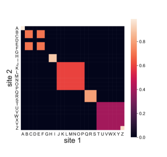
Figure S1: The cell values for the synthetic dataset with $L=2$ and $|{\mathcal{C}}^{\left({\ell}\right)}|=26\ \forall\ell\in\{1,2\}$.

References

- Bedbrook et al. (2017) Bedbrook, C. N., Yang, K. K., Rice, A. J., Gradinaru, V., and Arnold, F. H. Machine learning to design integral membrane channelrhodopsins for efficient eukaryotic expression and plasma membrane localization. PLoS computational biology, 13(10):e1005786, 2017.
- Chen & Krause (2013) Chen, Y. and Krause, A. Near-optimal batch mode active learning and adaptive submodular optimization. In International Conference on Machine Learning (ICML), June 2013.
- Desautels et al. (2014) Desautels, T., Krause, A., and Burdick, J. W. Parallelizing exploration-exploitation tradeoffs in gaussian process bandit optimization. The Journal of Machine Learning Research, 15(1):3873–3923, 2014.
- Guillory & Bilmes (2010) Guillory, A. and Bilmes, J. A. Interactive submodular set cover. In Proceedings of the 27th International Conference on Machine Learning (ICML-10), pp. 415–422, 2010.
- Hoi et al. (2006) Hoi, S. C. H., Jin, R., Zhu, J., and Lyu, M. R. Batch mode active learning and its application to medical image classification. In Proceedings of the 23rd international conference on Machine learning, ICML ’06, pp. 417–424, New York, NY, USA, 2006. ACM. ISBN 1-59593-383-2.
- Horst & Thoai (1999) Horst, R. and Thoai, N. V. Dc programming: overview. Journal of Optimization Theory and Applications, 103(1):1–43, 1999.
- Iyer & Bilmes (2012) Iyer, R. and Bilmes, J. Algorithms for approximate minimization of the difference between submodular functions, with applications. In Proceedings of the Twenty-Eighth Conference on Uncertainty in Artificial Intelligence, pp. 407–417. AUAI Press, 2012.
- Jegelka & Bilmes (2011) Jegelka, S. and Bilmes, J. Submodularity beyond submodular energies: coupling edges in graph cuts. In IEEE Conference on Computer Vision and Pattern Recognition (CVPR 2011), pp. 1897–1904. IEEE, 2011.
- Kauffman & Weinberger (1989) Kauffman, S. A. and Weinberger, E. D. The nk model of rugged fitness landscapes and its application to maturation of the immune response. Journal of theoretical biology, 141(2):211–245, 1989.
- Kempe et al. (2003) Kempe, D., Kleinberg, J., and Tardos, É. Maximizing the spread of influence through a social network. In Proceedings of the ninth ACM SIGKDD international conference on Knowledge discovery and data mining, pp. 137–146. ACM, 2003.
- Krause & Guestrin (2007) Krause, A. and Guestrin, C. Near-optimal observation selection using submodular functions. In AAAI, volume 7, pp. 1650–1654, 2007.
- Li et al. (2014) Li, M., Zhang, T., Chen, Y., and Smola, A. J. Efficient mini-batch training for stochastic optimization. In Proceedings of the 20th ACM SIGKDD international conference on Knowledge discovery and data mining, pp. 661–670. ACM, 2014.
- Narasimhan & Bilmes (2005) Narasimhan, M. and Bilmes, J. A submodular-supermodular procedure with applications to discriminative structure learning. In Proceedings of the Twenty-First Conference on Uncertainty in Artificial Intelligence, pp. 404–412. AUAI Press, 2005.
- Nemhauser et al. (1978) Nemhauser, G. L., Wolsey, L. A., and Fisher, M. L. An analysis of approximations for maximizing submodular set functions—i. Mathematical programming, 14(1):265–294, 1978.
- Podgornaia & Laub (2015) Podgornaia, A. I. and Laub, M. T. Pervasive degeneracy and epistasis in a protein-protein interface. Science, 347(6222):673–677, 2015.
- Rasmussen & Williams (2006) Rasmussen, C. E. and Williams, C. K. I. Gaussian Processes for Machine Learning. MIT Press, 2006.
- Romero et al. (2013) Romero, P. A., Krause, A., and Arnold, F. H. Navigating the protein fitness landscape with gaussian processes. Proceedings of the National Academy of Sciences, 110(3):E193–E201, 2013.
- Saito et al. (2018) Saito, Y., Oikawa, M., Nakazawa, H., Niide, T., Kameda, T., Tsuda, K., and Umetsu, M. Machine-learning-guided mutagenesis for directed evolution of fluorescent proteins. ACS synthetic biology, 2018. doi: 10.1021/acssynbio.8b00155.
- Srinivas et al. (2010) Srinivas, N., Krause, A., Kakade, S., and Seeger, M. Gaussian process optimization in the bandit setting: No regret and experimental design. In Proc. International Conference on Machine Learning (ICML), 2010.
- Voigt et al. (2001) Voigt, C. A., Mayo, S. L., Arnold, F. H., and Wang, Z.-G. Compuationally focusing the directed evolution of proteins. Journal of Cellular Biochemistry Supplement, 37:58–63, 2001.
- Wang et al. (2016) Wang, Z., Zhou, B., and Jegelka, S. Optimization as estimation with gaussian processes in bandit settings. In Artificial Intelligence and Statistics, pp. 1022–1031, 2016.
- Wu et al. (2016) Wu, N. C., Dai, L., Olson, C. A., Lloyd-Smith, J. O., and Sun, R. Adaptation in protein fitness landscapes is facilitated by indirect paths. Elife, 5:e16965, 2016.
- Wu et al. (2019) Wu, Z., Kan, S. B. J., Lewis, R. D., Wittmann, B. J., and Arnold, F. H. Machine-learning-assisted directed protein evolution with combinatorial libraries. arXiv preprint arXiv:1902.07231, 2019.
- Yang & Carbonell (2013) Yang, L. and Carbonell, J. Buy-in-bulk active learning. In Advances in Neural Information Processing Systems, pp. 2229–2237, 2013.
- Zinkevich et al. (2010) Zinkevich, M., Weimer, M., Li, L., and Smola, A. J. Parallelized stochastic gradient descent. In Advances in neural information processing systems, pp. 2595–2603, 2010.