The period–luminosity relation for $\delta$ Scuti stars using Gaia DR2 parallaxes

Abstract

We have examined the period–luminosity (P–L) relation for $\delta$ Scuti stars using Gaia DR2 parallaxes. We included 228 stars from the catalogue of Rodriguez et al. (2000), as well as 1124 stars observed in the four-year Kepler mission. For each star we considered the dominant pulsation period, and used DR2 parallaxes and extinction corrections to determine absolute $V$ magnitudes. Many stars fall along a sequence in the P–L relation coinciding with fundamental-mode pulsation, while others pulsate in shorter-period overtones. The latter stars tend to have higher effective temperatures, consistent with theoretical calculations. Surprisingly, we find an excess of stars lying on a ridge with periods half that of the fundamental. We suggest this may be due to a 2:1 resonance between the third or fourth overtone and the fundamental mode.

1 Introduction

Period–luminosity (P–L) relations of pulsating stars have a long and distinguished history (Leavitt & Pickering, 1912). They arise when a class of pulsating stars occupies a relatively narrow range of effective temperatures, in which case luminosity correlates quite strongly with stellar density, and hence with the pulsation periods of pressure modes (e.g., Eddington, 1926; Carroll & Ostlie, 2006). In this paper, we investigate the P–L relation for the $\delta$ Scuti class of pulsating stars using parallaxes from Gaia DR2 (Gaia Collaboration, 2018).

The $\delta$ Sct stars are intermediate-mass stars with spectral types A2V to F2V that pulsate in low-order pressure modes. They are located within an interesting region in the Hertzprung-Russell (HR) diagram, between low-mass stars having thick convective envelopes ($\leq 1M_{\sun}$) and high-mass stars with large convective cores and radiative envelopes ($\geq 2M_{\sun}$). They lie in the lower part of the classical instability strip, within or just above the main sequence in HR diagram, with effective temperatures between approximately 6400 K and 8600 K and pulsation frequencies above 5 d^-1, often with multiple periodicities (e.g., Breger, 2000; Michel et al., 2017; Balona, 2018; Bowman & Kurtz, 2018; Pamyatnykh, 2000; Qian et al., 2018).

In $\delta$ Sct stars, pulsations are excited by the well-known $\kappa$ mechanism, which operates in zones of partial ionization of hydrogen and helium. In cooler $\delta$ Sct stars with substantial outer convection zones, the selection mechanism of modes with observable amplitudes could be affected by induced fluctuations of the turbulent convection. A theoretical blue edge of the instability strip for radial and non-radial modes was determined by Pamyatnykh (2000). At the red edge, pulsation is damped by convection such that a non-adiabatic treatment of the interaction between convection and pulsation is required, in so-called time dependent convection (TDC) models. Houdek (2000) and Xiong & Deng (2001) used TDC to study the red edge of radial modes, while a red edge for non-radial modes was produced three years later by Dupret et al. (2004). TDC has an adjustable mixing length parameter, $\alpha_{\rm MLT}$, whose value influences the position of both the blue and red edges. Dupret et al. (2005) calculated instability strips of radial and non-radial modes for different values of $\alpha_{\rm MLT}$.

Like RR Lyraes and Cepheids, which also lie in the instability strip, the $\delta$ Sct stars are known to follow a P–L relation, at least for high-amplitude pulsators and admittedly with considerable scatter (e.g., Breger & Bregman, 1975; King, 1991; North et al., 1997; McNamara, 1997; Poretti et al., 2008; Garg et al., 2010; Poleski et al., 2010; McNamara, 2011; Cohen & Sarajedini, 2012). In particular, McNamara (2011) studied the P–L relation of high-amplitude $\delta$ Sct stars and used it to find the distance moduli of three galaxies and two globular clusters. In this paper we revisit the P–L relation for $\delta$ Sct stars using Gaia DR2 parallaxes, considering only the highest-amplitude mode in each star. It is important to keep in mind that $\delta$ Sct stars can pulsate in fundamental modes ($n=1$) and also in overtone modes ($n=2,3,4,\ldots$), and that these modes can be either radial ($l=0$) or nonradial ($l=1,2,\ldots$). In general, if the strongest oscillation mode in a star falls on the P–L relation, it is likely to be the radial fundamental mode ($n=1$, $l=0$) or possibly a low-order dipole mode ($l=1$), while other modes are expected to have shorter periods.

In Section 2 we describe our sample’s construction. In Section 3 the P–L diagrams are plotted, and possible explanations for the P–L relation are discussed in Section 4.

2 Construction of samples

2.1 Rodriguez et al. (2000) catalogue

Rodríguez et al. (2000) catalogued the dominant pulsation period for 636 $\delta$ Sct stars. Based on the list of rejected $\delta$ Sct stars in Table 5 of Liakos & Niarchos (2017), three stars from the catalogue (BQ Phe, DE Oct, V345 Gem) were identified as binaries with no pulsating components and removed from our sample. We also removed AK Men as a binary after light curve inspection. Fourteen stars from crowded parts of sky were removed because their coordinates were not precise enough to reliably query against dust maps (e.g. Green et al., 2015). A further six stars (HD 302013 = V753 Cen, HD 358431 = YZ Cap, TV Lyn, BP Peg, DH Peg, and UY Cam) were excluded for being RR Lyrae stars (e.g., Sneden et al., 2018; McNamara, 2011). We also dropped the B-type $\beta$ Cep variable, V1228 Cen (Pigulski & Pojmański, 2008). Two further stars without measured parallaxes were also discarded (HD 23567 = V534 Tau and 2MASS J13554648-291123).

We also included four bright $\delta$ Sct stars that were recently discovered, and are therefore not in the Rodríguez et al. (2000) catalogue (shown by cyan triangles in Figs. 1 and 3):

• Altair ($\alpha$ Aql) was found to be the brightest $\delta$ Sct star in the sky ($V=0.76$) by Buzasi et al. (2005) using WIRE photometry, with a dominant frequency of 15.77 d^-1. It is included in Fig. 1 of McNamara (2011).

• $\beta$ Pic has a dominant frequency of 47.4 d^-1, based on photometry from Antarctica (Mékarnia et al., 2017).

• 95 Vir has a dominant frequency of 9.537 d^-1, based on Kepler K2 photometry (Paunzen et al., 2017).

• $\eta$ Ind (HR 7920) has a dominant frequency of 26.5 d^-1, although this could be affected by daily aliases (Koen et al., 2017).

We calculated the absolute magnitudes for all these stars using

$$M_{V}=V+5\log\pi+5-A_{V},$$ (1)

where $M_{V}$ and $V$ denote the absolute and apparent magnitudes in the $V$ band, respectively, $\pi$ is the parallax in arcsec, and $A_{V}$ is the extinction due to interstellar dust. We used parallaxes from Gaia DR2 except for a few cases where the Hipparcos parallaxes were more precise. We calculated $A_{V}$ using the dust map by Green et al. (2015).

2.2 Kepler $\delta$ Sct stars

Many $\delta$ Sct stars were observed by Kepler during its four-year nominal mission (e.g., Balona & Dziembowski, 2011; Balona et al., 2015; Bradley et al., 2015; Moya et al., 2017; Balona, 2018; Barceló Forteza et al., 2018; Bowman & Kurtz, 2018). We have used the sample of about 2000 $\delta$ Sct stars identified by Murphy et al. (2019) from Kepler long-cadence data. To account for the averaging of pulsations during the 29.4-minute integrations ($f_{\rm Nyq}=24.5\,\mbox{d${}^{-1}$}$), we divided the observed amplitudes in the Fourier spectrum by the function $\operatorname{sinc}\left(\frac{\pi}{2}\frac{f}{f_{\rm Nyq}}\right)$ (e.g., Huber et al., 2010). We measured the dominant period in each star from the highest peak in the Fourier spectrum in the range of 0.0228 to 0.2 days (i.e., with frequencies from 5 to 43.9 d^-1).

We calculated the absolute magnitudes for the stars in the Kepler sample using

$$M_{V}=V-5\log d+5-A_{V},$$ (2)

where $M_{V}$ and $V$ denote the absolute and apparent magnitudes in the $V$ band, respectively, $d$ is the distance in pc, and $A_{V}$ is the extinction due to interstellar dust. Apparent magnitudes were obtained from Everett et al. (2012), accessed via MAST (V_UBV) and assigned an uncertainty of 0.05 mag. To obtain stellar distances from Gaia DR2 parallaxes, we used the normalised posterior distribution and adopted length scale model of Bailer-Jones et al. (2018). This approach is advantageous, as it allows for a Bayesian approach to distance estimation. This produces a distribution of distances from which Monte Carlo samples can be drawn. Extinctions and their uncertainties were obtained with the dustmaps Python package (Green, 2018), which provides access to the Bayestar 17 reddening map of Green et al. (2018). To convert to the appropriate photometric system (Johnson V), we used the extinction coefficient in Table A1 of Sanders & Das (2018). A small recommended grey offset of 0.063 was introduced into the extinctions. We determined the magnitude and its associated uncertainty for each star with a Monte-Carlo process, taking the mean value of 200 000 samples for the magnitude, and the 1-$\sigma$ standard deviation for the uncertainty.

3 Period–Luminosity Diagram

To study the P–L relation with high accuracy, we preferentially chose stars with good parallaxes and reasonably small extinction corrections. For the Rodríguez et al. (2000) catalogue, we used 228 stars with $V<14$ mag, fractional parallax uncertainties less than 5 percent (translating to uncertainties less than 0.11 mag in $M_{V}$) and $A_{V}<0.2$. For the Kepler sample, we used 1124 stars with fractional parallax uncertainties less than 5 percent and $A_{V}<0.5$.

It is known that some $\delta$ Sct stars show amplitude variability (see Bowman et al., 2016, and references therein), even to the extent that the dominant mode (that is, the mode having the highest amplitude) might vary with time. This would introduce some horizontal scatter in the P–L diagram. Meanwhile, the light variations in high-amplitude $\delta$ Sct stars (HADS) can reach a few tenths of a magnitude, which could lead to some additional scatter in the vertical direction.

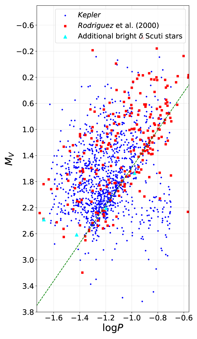
Figure 1: Period–luminosity diagram of $\delta$ Sct stars having fractional parallax uncertainties less than 5 percent. Blue dots are 1124 $\delta$ Sct stars in the Kepler field and red squares are 228 stars from the $\delta$ Sct catalogue of Rodríguez et al. (2000). The cyan triangles indicate the four additional bright $\delta$ Sct stars discussed in Sec. 2.1, which are (from left to right) $\beta$ Pic, $\eta$ Ind, Altair and 95 Vir. The diagonal dashed green line shows the relation from McNamara (2011, see Eq. 3).

Figure 2: The distance of data points to the McNamara line as a histogram. Red: 228 $\delta$ Sct stars from the Rodríguez et al. catalogue corrected for extinction by the Green et al. (2015) dust map. Blue: 1124 $\delta$ Sct stars from Kepler, corrected for extinction by the Green et al. (2018) dust map.

Figure 1 shows our resulting P–L relation. Red squares are stars from Rodríguez et al. (2000) catalogue, blue circles are Kepler stars and cyan triangles are the additional stars mentioned in 2.1. The diagonal green line is the P–L relation derived by McNamara (2011) for the high-amplitude $\delta$ Sct stars, which are thought to pulsate in their radial fundamental mode.

We see that many stars fall in a ridge close to the dashed line. Note that the group of Kepler stars in the lower right of Fig. 1, whose periods appear to be too long for $\delta$ Sct pulsations, are mostly $\gamma$ Dor stars with harmonics above 5 d^-1 in the Fourier spectrum (see Murphy et al., 2019).

Many stars in Fig. 1 lie to the left of the fundamental ridge, indicating that their dominant pulsation period corresponds to an overtone mode. Surprisingly, there appears to be an excess of stars in a second ridge that lies to the left of the main ridge. To make this clearer, we show in Fig. 2 the histogram of horizontal distances from the fundamental-mode ridge. That is, the red histogram shows the horizontal distances (in $\log P$) from the McNamara (2011) line of stars in the Rodríguez et al. (2000) sample, while the blue histogram shows the same for the Kepler stars. The main peak (at zero distance in $\log P$) corresponds to the fundamental-mode ridge. The second peak is clearly visible in both samples, and indicates that this ridge is displaced horizontally by 0.3 in $\log P$, corresponding to a period ratio of ($10^{-0.3}$ =) 0.50. Thus, it appears that a significant number of stars in both samples have a dominant pulsation period that is half that of the fundamental mode.

Our two samples are somewhat different, given that the Rodríguez et al. (2000) catalogue comprises ground-based data, often from relatively short observations, whereas Kepler observed from space for four years. To make the comparison more similar, we plotted the histogram after restricting the Kepler sample to stars with semi-amplitudes (measured in the Fourier transform) above 1 mmag. The result is shown in Fig. 3. The histograms for the two samples do indeed appear to be more similar, although there are still some differences. The main point is the two ridges separated by a factor of two in period appear in both samples.

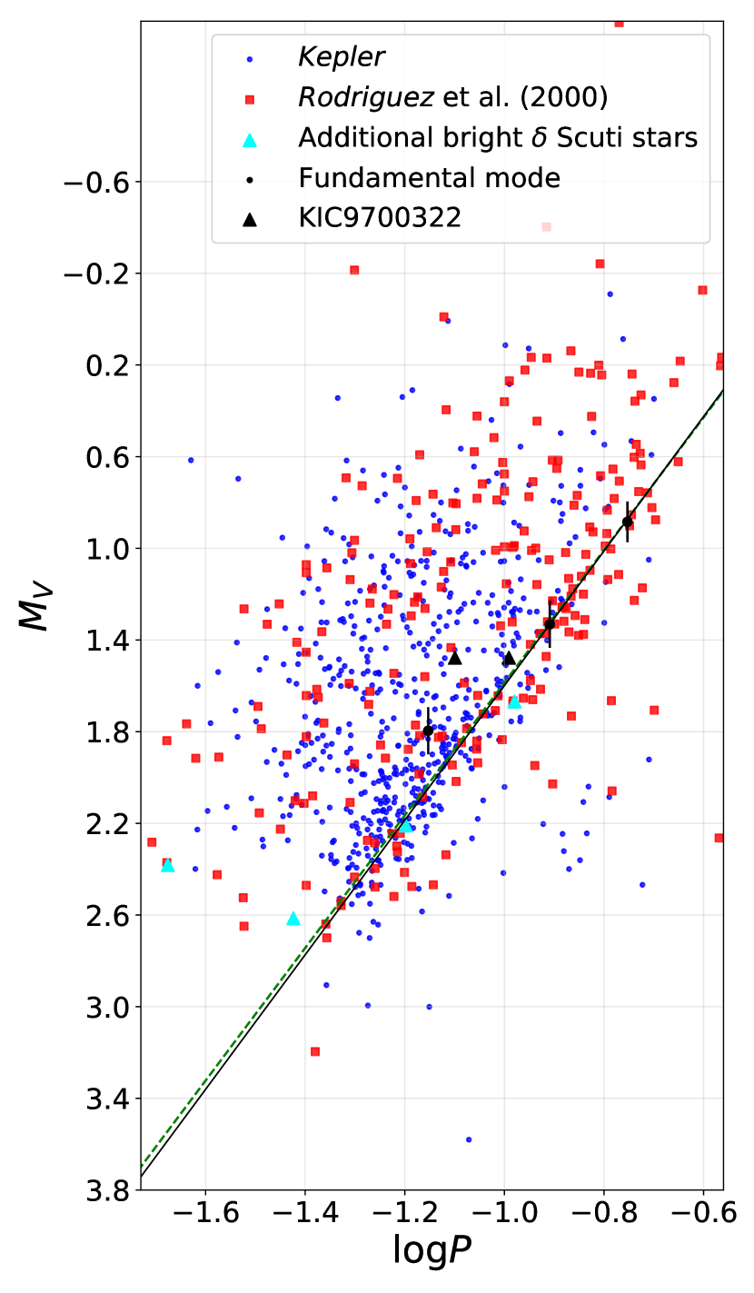
Figure 3: Same as Fig. 1, except that the Kepler sample (blue dots) is restricted to 601 stars having a pulsation semi-amplitude above 1 mmag, and an offset of 0.125 mag has been subtracted from $V$ magnitudes for the Kepler sample (see text). The diagonal lines show the McNamara relation (dashed green line; see Eq. 3) and our new fit (solid black line; see Eq. 4). Three Kepler stars for which the dominant mode has been identified as the radial fundamental are marked by black circles, with error bars. From left to right, they are KIC 5950759, KIC 2304168 and KIC 9408694 (V2367 Cyg). The black triangles show the two strongest modes in KIC 9700322, the left one corresponding to the first radial overtone (the dominant mode) and the right one being the fundamental radial mode (Breger et al., 2011)

.

Figure 4: Same as Fig. 2, except applied to the P–L diagram in Fig. 3.

A fit to the P–L relation for a small number of $\delta$ Sct stars was made by McNamara (2011), who found that

$$M_{V}=(-2.89\pm 0.13)\log P-(1.31\pm 0.10).$$ (3)

This is shown as the green dashed line in Figs. 1 and 3. In order to determine a revised equation for this P–L relation, we fitted to all stars in both samples that are located on the fundamental ridge. The fitted line is shown by the black solid line in Fig. 3 and has the following equation:

$$M_{V}=(-2.94\pm 0.06)\log P-(1.34\pm 0.06).$$ (4)

This is very similar to the line fitted by McNamara (2011).

4 Discussion

The results indicate that the dominant period in most $\delta$ Sct stars lies on the ridge that coincides with the fundamental mode. This does not necessarily mean that the dominant mode is the radial fundamental in every one of these stars, since it could also be a low-order nonradial mode. Nevertheless, the diagram should prove useful when trying to identify the other modes in multi-periodic pulsators. For example, three of the additional stars mentioned in Sec. 2.1 (cyan triangles in Figs. 1 and 3) appear to fall into this class (Altair, 95 Vir and $\eta$ Ind). In other stars (including the fourth additional star, $\beta$ Pic) the dominant mode has a period much shorter than the fundamental, corresponding to an overtone mode ($n>1$).

In Fig. 3 we indicate three Kepler $\delta$ Sct stars (black points with error bars) for which the dominant pulsation mode has been identified as the fundamental radial mode: KIC 5950759 (Bowman et al. 2016; $\log P=-1.15$), KIC 2304168 (Balona & Dziembowski 2011; $\log P=-0.91$), and V2367 Cyg (KIC 9408694; Balona et al. 2012; $\log P=-0.75$). These stars all lie close to the main ridge, as expected. Note that we have included error bars (see Sec. 2.2 for details) as an indication of the typical precision in $M_{V}$ for the Kepler sample.

In Fig. 3 we also show the two strongest modes in KIC 9700322, which were identified by Breger et al. (2011) as radial modes (black triangles). The shorter-period mode, which has a slightly higher amplitude and is therefore the dominant mode, corresponds to the first overtone. The longer-period mode (which should not really be plotted in the figure because it is not the dominant mode) is the radial fundamental and lies on the main ridge, as expected, while the period of the first overtone is a shorter by a factor of $0.78$ (shifted by $-0.11$ in $\log P$).

4.1 Stars in the lower-right of the P–L diagram

Some points in Fig. 3 lie well to the lower-right of the main ridge. As discussed above, those from the Kepler sample are explained as harmonics in the Fourier spectrum of gravity modes ($\gamma$ Dor pulsations). For the Rodríguez et al. (2000) catalogue (red squares), we have checked the seven stars that fall furthest to the lower-right in the diagram. For four of these stars, subsequent publications have shown that the period in the catalogue is not from $\delta$ Sct pulsations:

• AD Ari ($\log P=-0.57$, $M_{V}=2.26$) is an ellipsoidal variable (Handler & Shobbrook, 2002);

• $\epsilon$ UMa ($\log P=-0.90$, $M_{V}=2.03$) is a rotating magnetic Ap star (Shulyak et al., 2010);

• V1241 Tau ($\log P=-0.78$, $M_{V}=2.06$) is an eclipsing binary (Arentoft et al., 2004); and

• V831 Her ($\log P=-0.94$, $M_{V}=1.95$) is a constant star within the instability strip (Henry et al., 2011).

These examples demonstrate the usefulness of the P–L diagram for identifying misclassified stars. For the other three stars, the situation is less clear:

• BX Scl (CS 22966$-$0043; $\log P=-1.43$, $M_{V}=3.84$) is at the faint limit of our sample ($V=13.56$). It is an SX Phe pulsator and possibly an usual type of blue straggler (Preston & Landolt, 1998), which may explain its anomalous position.

• FP Ser (=40 Ser; $\log P=-0.70$, $M_{V}=1.71$) has a period of 0.20 d in the catalogue, which comes from Jackisch (1972). That paper actually suggests a period of 5–6 hours, based on observations over four nights in 1965, and it is clearly desirable to confirm this period.

• GS UMa ($\log P=-0.79$, $M_{V}=1.66$) has a period of 0.164 d from Hipparcos data, which was recently confirmed by Kahraman Alicavus et al. (2018). However, those authors noted that GS UMa is cooler than the red edge of the instability strip, and its position in Fig. 3 implies it may be a $\gamma$ Dor pulsator rather than a $\delta$ Sct star.

Data from the TESS Mission should help test these conclusions and clarify the classifications of these stars.

4.2 Interpretation of the P–L diagram

Theoretical models by Dziembowski (1997), Houdek et al. (1999) and Dupret et al. (2005) indicate that the fundamental mode is unstable (i.e. excited) in stars on the cooler side of the instability strip, but that excitation shifts to progressively higher overtones at higher effective temperatures (see also Xiong & Deng 2001; Xiong et al. 2016). To investigate this further, we show an HR diagram in Fig. 5 for the Kepler $\delta$ Sct stars, where the colour indicates the horizontal distance from the fundamental P–L relation. We clearly see that an increase in effective temperature correlates with the dominant period being shorter than the fundamental, which is consistent with a higher-order overtone being dominant. This is also consistent with findings that Kepler $\delta$ Sct stars with higher $T_{\rm eff}$ tend to have shorter dominant periods, i.e. a higher $\nu_{\rm max}$ (Balona & Dziembowski, 2011; Barceló Forteza et al., 2018).

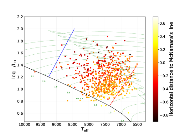
Figure 5: HR diagram for our sample of Kepler $\delta$ Sct stars having fractional parallax uncertainties less than 5 percent and pulsation semi-amplitudes above 1 mmag. Luminosities and temperatures are taken from Murphy et al. (2019). The colour indicates the horizontal distance from the fundamental-mode relation in the P–L diagram (Fig. 4), with redder colours corresponding to shorter periods (higher pulsation overtones). The evolutionary tracks (green) are from Murphy et al. (2019) and have X = 0.71 and Z = 0.014. The blue and red lines are the theoretical instability strip boundaries using TDC and $\alpha_{\rm MLT}=1.8$ from Dupret et al. (2005).

The puzzling finding from this work is the second ridge in the P–L diagram (Figs. 1 to 4). One possibility is that the second ridge is displaced vertically, in absolute magnitude, due to binarity. However, the vertical displacement is 0.9 mag, higher than the 0.75 mag expected for a binary sequence of equal-luminosity components. This difference is larger still, since $\delta$ Sct stars preferentially have low-mass (low-luminosity) companions (Murphy et al., 2018). Also, the 72 stars in the Rodríguez et al. (2000) sample that are listed as binary systems by Liakos & Niarchos (2017) do not preferentially lie on the second sequence. We consider it more likely that the second ridge is displaced horizontally, to shorter periods. The tendency of the shorter-period stars to have higher effective temperatures (Fig. 5) is consistent with this, as discussed above. However, the excess of stars having a dominant period that is half the fundamental needs an explanation.

Could the second ridge correspond to the second harmonic of the fundamental mode? It is common for $\delta$ Sct stars to show combination frequencies, and a strong peak at frequency $f$ in the Fourier transform is often accompanied by a peak at twice that frequency. However, in most cases the peak at $2f$ is much smaller in amplitude, and it would not appear in our P–L diagrams.

We are left to propose that the dominant period of the stars on the second ridge is an overtone that is excited to higher-than-expected amplitude due to a 2:1 resonance with the fundamental, even though the fundamental mode itself is not unstable. Resonances are well known in pulsating stars (e.g., Buchler et al., 1997; Kolláth et al., 2011; Breger & Montgomery, 2014; Barceló Forteza et al., 2015; Bowman et al., 2016), and so it seems at least plausible that such a mechanism may boost the third or fourth overtone so that it becomes the dominant mode in cases where its frequency is twice that of the fundamental. We encourage theoretical investigations of this possibility.

5 Conclusions

By using the Gaia DR2 parallaxes, we have examined the P–L relation for $\delta$ Sct stars. In the current work, two samples of $\delta$ Sct stars were constructed (see Sec. 2), the first containing 228 stars from ground-based observations catalogued by Rodríguez et al. (2000) and the second including 1124 stars observed by Kepler. The absolute magnitude of each star was calculated by using Gaia DR2 parallaxes, including a correction for extinction, and then was plotted against the dominant period of the star (see Sec. 3).

Figure 3 shows the P–L relation for both samples, where only those Kepler stars with semi-amplitudes above 1 mmag are included. In this figure, many stars fall in a ridge very close to the green dashed line, which corresponds to the published P–L relation of the radial fundamental mode in $\delta$ Sct stars. The general distribution is in agreement with theoretical models, which indicate the excited mode in a hotter $\delta$ Sct star would shift to higher overtones (see Fig. 5).

There is an excess of stars in a second ridge for both samples, to the left of the main ridge by a distance of 0.3 in $\log P$, that could also be distinguished in histograms (Figs. 2 and 4). This ridge corresponds to stars having a dominant period that is half that of the main ridge. We suggest that this may be an excited overtone that is boosted by a 2:1 resonance with the fundamental. In future work, detailed examination of the Fourier Transforms of Kepler light curves could give us more information about the pulsation modes of the stars in the second ridge.

References

- Arentoft et al. (2004) Arentoft T., Lampens P., Van Cauteren P., Duerbeck H. W., García-Melendo E., Sterken C., 2004, A&A, 418, 249
- Bailer-Jones et al. (2018) Bailer-Jones C. a. L., Rybizki J., Fouesneau M., Mantelet G., Andrae R., 2018, The Astronomical Journal, 156, 58
- Balona (2018) Balona L. A., 2018, MNRAS, 479, 183
- Balona & Dziembowski (2011) Balona L. A., Dziembowski W. A., 2011, MNRAS, 417, 591
- Balona et al. (2012) Balona L. A., et al., 2012, MNRAS, 419, 3028
- Balona et al. (2015) Balona L. A., Daszyńska-Daszkiewicz J., Pamyatnykh A. A., 2015, MNRAS, 452, 3073
- Barceló Forteza et al. (2015) Barceló Forteza S., Michel E., Roca Cortés T., García R. A., 2015, A&A, 579, A133
- Barceló Forteza et al. (2018) Barceló Forteza S., Roca Cortés T., García R. A., 2018, A&A, 614, A46
- Bowman & Kurtz (2018) Bowman D. M., Kurtz D. W., 2018, MNRAS, 476, 3169
- Bowman et al. (2016) Bowman D. M., Kurtz D. W., Breger M., Murphy S. J., Holdsworth D. L., 2016, MNRAS, 460, 1970
- Bradley et al. (2015) Bradley P. A., Guzik J. A., Miles L. F., Uytterhoeven K., Jackiewicz J., Kinemuchi K., 2015, AJ, 149, 68
- Breger (2000) Breger M., 2000, in ASP Conf. Series, Vol. 210. p. 3
- Breger & Bregman (1975) Breger M., Bregman J. N., 1975, ApJ, 200, 343
- Breger & Montgomery (2014) Breger M., Montgomery M. H., 2014, ApJ, 783, 89
- Breger et al. (2011) Breger M., et al., 2011, MNRAS, 414, 1721
- Buchler et al. (1997) Buchler J. R., Goupil M.-J., Hansen C. J., 1997, A&A, 321, 159
- Buzasi et al. (2005) Buzasi D. L., et al., 2005, ApJ, 619, 1072
- Carroll & Ostlie (2006) Carroll B. W., Ostlie D. A., 2006, An Introduction to Modern Astrophysics. San Francisco: Pearson, Addison-Wesley
- Cohen & Sarajedini (2012) Cohen R. E., Sarajedini A., 2012, MNRAS, 419, 342
- Dupret et al. (2004) Dupret M.-A., Grigahcène A., Garrido R., Gabriel M., Scuflaire R., 2004, A&A, 414, L17
- Dupret et al. (2005) Dupret M.-A., Grigahcène A., Garrido R., Gabriel M., Scuflaire R., 2005, A&A, 435, 927
- Dziembowski (1997) Dziembowski W., 1997, in Provost J., Schmider F.-X., eds, IAU Symposium Vol. 181, Sounding Solar and Stellar Interiors. p. 317
- Eddington (1926) Eddington A. S., 1926, The Internal Constitution of the Stars. Cambridge: Cambridge University Press
- Everett et al. (2012) Everett M. E., Howell S. B., Kinemuchi K., 2012, PASP, 124, 316
- Gaia Collaboration (2018) Gaia Collaboration 2018, A&A, 616, A1
- Garg et al. (2010) Garg A., et al., 2010, AJ, 140, 328
- Green (2018) Green G. M., 2018, The Journal of Open Source Software, 3, 695
- Green et al. (2015) Green G. M., et al., 2015, ApJ, 810, 25
- Green et al. (2018) Green G. M., et al., 2018, MNRAS, 478, 651
- Handler & Shobbrook (2002) Handler G., Shobbrook R. R., 2002, MNRAS, 333, 251
- Henry et al. (2011) Henry G. W., Fekel F. C., Henry S. M., 2011, AJ, 142, 39
- Houdek (2000) Houdek G., 2000, in Breger M., Montgomery M., eds, Astronomical Society of the Pacific Conference Series Vol. 210, Delta Scuti and Related Stars. p. 454
- Houdek et al. (1999) Houdek G., Balmforth N. J., Christensen-Dalsgaard J., Gough D. O., 1999, A&A, 351, 582
- Huber et al. (2010) Huber D., et al., 2010, ApJ, 723, 1607
- Jackisch (1972) Jackisch G., 1972, Astronomische Nachrichten, 294, 1
- Kahraman Alicavus et al. (2018) Kahraman Alicavus F., Raheem A., Coban G. C., Tambulut E. M., Gogulter U., BAS L., Cevirici B., 2018, Information Bulletin on Variable Stars, 6246, 1
- King (1991) King J. R., 1991, Information Bulletin on Variable Stars, 3562
- Koen et al. (2017) Koen C., van Wyk F., Laney C. D., Kilkenny D., 2017, MNRAS, 466, 122
- Kolláth et al. (2011) Kolláth Z., Molnár L., Szabó R., 2011, MNRAS, 414, 1111
- Leavitt & Pickering (1912) Leavitt H. S., Pickering E. C., 1912, Harvard College Observatory Circular, 173, 1
- Liakos & Niarchos (2017) Liakos A., Niarchos P., 2017, MNRAS, 465, 1181
- McNamara (1997) McNamara D., 1997, PASP, 109, 1221
- McNamara (2011) McNamara D. H., 2011, AJ, 142, 110
- Mékarnia et al. (2017) Mékarnia D., et al., 2017, A&A, 608, L6
- Michel et al. (2017) Michel E., et al., 2017, in EPJWC. p. 03001 (arXiv:1705.03721)
- Moya et al. (2017) Moya A., Suárez J. C., García Hernández A., Mendoza M. A., 2017, MNRAS, 471, 2491
- Murphy et al. (2018) Murphy S. J., Moe M., Kurtz D. W., Bedding T. R., Shibahashi H., Boffin H. M. J., 2018, MNRAS, 474, 4322
- Murphy et al. (2019) Murphy S. J., Hey D., Van Reeth T., Bedding T. R., 2019, MNRAS (submitted)
- North et al. (1997) North P., Jaschek C., Egret D., 1997, in Bonnet R. M., et al., eds, ESA Special Publication Vol. 402, Hipparcos – Venice ’97. p. 367
- Pamyatnykh (2000) Pamyatnykh A. A., 2000, in Breger M., Montgomery M., eds, Astronomical Society of the Pacific Conference Series Vol. 210, Delta Scuti and Related Stars. p. 215 (arXiv:astro-ph/0005276)
- Paunzen et al. (2017) Paunzen E., Hümmerich S., Bernhard K., Walczak P., 2017, MNRAS, 468, 2017
- Pigulski & Pojmański (2008) Pigulski A., Pojmański G., 2008, A&A, 477, 907
- Poleski et al. (2010) Poleski R., et al., 2010, Acta Astron., 60, 1
- Poretti et al. (2008) Poretti E., et al., 2008, ApJ, 685, 947
- Preston & Landolt (1998) Preston G. W., Landolt A. U., 1998, AJ, 115, 2515
- Qian et al. (2018) Qian S.-B., Li L.-J., He J.-J., Zhang J., Zhu L.-Y., Han Z.-T., 2018, MNRAS, 475, 478
- Rodríguez et al. (2000) Rodríguez E., López-González M. J., López de Coca P., 2000, A&AS, 144, 469
- Sanders & Das (2018) Sanders J. L., Das P., 2018, arXiv:1806.02324 [astro-ph]
- Shulyak et al. (2010) Shulyak D., Krtička J., Mikulášek Z., Kochukhov O., Lüftinger T., 2010, A&A, 524, A66
- Sneden et al. (2018) Sneden C., et al., 2018, AJ, 155, 45
- Xiong & Deng (2001) Xiong D. R., Deng L., 2001, MNRAS, 324, 243
- Xiong et al. (2016) Xiong D. R., Deng L., Zhang C., Wang K., 2016, MNRAS, 457, 3163