Probing Boson Stars with Extreme Mass Ratio Inspirals
Abstract
We propose to use gravitational waves from extreme mass ratio inspirals (EMRI), composed of a boson star and a supermassive black hole in the center of galaxies, as a new method to search for boson stars. Gravitational waves from EMRI have the advantage of being long-lasting within the frequency band of future space-based interferometer gravitational wave detectors and can accumulate large signal-to-noise ratio (SNR) for very sub-solar mass boson stars. Compared to gravitational waves from boson star binaries, which fall within the LIGO band, we find that much larger ranges of the mass and compactness of boson stars, as well as the underlying particle physics parameter space, can be probed by EMRI. We take tidal disruption of the boson stars into account and distinguish those which dissolve before the inner-most-stable-circular-orbit (ISCO) and those which dissolve after it. Due to the large number of cycles recorded, EMRIs can lead to a very precise mass determination of the boson star and distinguish it from standard astrophysical compact objects in the event of a signal. Tidal effects in inspiralling binary systems, as well as possible correlated electromagnetic signals, can also serve as potential discriminants.
1 Introduction
Light scalars with long de Broglie wavelengths and suppressed couplings to the Standard Model can form gravitationally bound Bose-Einstein condensates (BEC) leading to macroscopic objects called boson stars Colpi:1986ye ; Tkachev:1986tr ; vanderBij:1987gi . The study of such condensates has a rich history in the context of early Universe cosmology. Analytic and numerical investigations pertaining to the evolution, stability, and decay of boson stars have been undertaken by various groups (we refer to JetzerP ; Schunck:2003kk ; Liebling:2012fv for reviews). These questions are also of interest to particle physicists, given the central place that light fundamental scalars occupy in theories beyond the Standard Model. The hope is that astrophysical constraints on boson stars will translate into constraints on the scalar field itself, such as its mass and interactions.
Gravitational waves Abbott:2016blz can play a significant role in these questions. The general idea is that for macroscopic exotic compact objects (ECOs) formed of light bosons, with masses comparable to stellar black holes and compactness sufficiently large that a binary system can form, gravitational wave signals will be generated. Current and future gravitational wave detectors can constrain the mass and compactness of the ECOs. Since these attributes are in turn determined by the physics at the microscopic scale such as the mass and self-interaction of the field, the probed regions of the mass-compactness plane will shed light on the underlying particle physics parameters. Several cases have been pursued by different groups: mergers of mini-boson and solitonic boson stars 1989PhRvL..63.1199G ; Palenzuela:2006wp ; Palenzuela:2007dm ; Amin:2013eqa ; Bezares:2018qwa , oscillations Helfer:2018vtq , Proca stars Sanchis-Gual:2018oui , and repulsive boson stars Croon:2018ybs ; Croon:2018ftb . These studies focused on binary systems with comparable masses, similar to stellar black holes, which produce gravitational waves within the band of LIGO Giudice:2016zpa .
The purpose of this paper is to point out that extreme mass ratio inspirals (EMRI) are very effective in probing boson stars and future space-based interferometers which target EMRI can potentially constrain a large part of the mass versus compactness parameter space. The standard EMRI consists of a stellar black hole, neutron star or white dwarf circling around a supermassive black hole (SMBH) at the center of each galaxy. ECOs, if they exist, can also create EMRI systems and constitute an entirely new target species for space-based gravitational wave detectors. Compared to the binary system detected by LIGO, an ECO can linger around the inner-most-stable-circular-orbit (ISCO) of the SMBH for a very long time and accumulate a large signal-to-noise ratio (SNR) in the LISA band even it has very sub-solar mass. Another factor further enhances the SNR: since astrophysical observations suggest that the spins of SMBHs in galaxies tend to have a value very close to 1, this results in a decreased radius of the ISCO and allows the ECOs to be closer to the SMBH, leading to larger SNR.
An important aspect of our work is to stress that in the event of a discovery, EMRIs would naturally allow for an unambiguous identification of the participant as an ECO and not a standard astrophysical compact object. Due to the large number of cycles recorded, even for very sub-solar ECOs, EMRIs can lead to a very precise determination of the parameters in the system, such as the masses of the SMBH and the boson star, and the SMBH spin, with errors as small as Barack:2003fp ; Klein:2015hvg . Therefore if gravitational waves are observed from an EMRI system and it is determined that the smaller object has sub-solar mass, this would definitely rule out the possibility of impostors like stellar black holes, neutron stars or white dwarfs. In particular, for those ECOs that are disrupted before reaching ISCO, we can also estimate their radius (hence compactness) to break the degeneracy with primordial black holes. Moreover, tidal effects in inspiralling binary systems, as well as possible correlated electromagnetic signals, can also serve as a potential discriminant between ordinary compact objects and boson stars.
The typically large SNR for even very sub-solar mass ECOs thus provides an extensive probe of the ECO parameter space, extending the coverage of mass and compactness to much lower regions, and serves as a powerful probe of the underlying particle physics.
Before proceeding, we note that in our work we remain agnostic about the connection between dark matter and boson stars, an aspect that has been explored by several authors. In particular, we do not impose dark matter constraints on the particle physics model, except that we require the scalar to be complex so that it has conserved particle number, massive, and having repulsive quartic interaction. Our aim is to present a case for using EMRIs to probe boson stars, and we study this case using a phenomenological model. The drawback in such an approach is that it is then difficult to provide the predicted EMRI event rate, since abundances are free to vary. We briefly provide an event rate estimation in Section 4, assuming that ECOs constitute the entire dark matter halo at the center of the galaxy, although we do not further explore the consequences of such an assumption in our model, at the level of the particle physics.
The paper is organized as follows. We start with a description of boson stars in Section 2, where we discuss the phenomenological model and compute the profile of the boson star in the mass-compactness plane. We then discuss the EMRI system as well as gravitational waves from such systems in Section 3. In Section 4, we show the results of our analysis, including the region of boson star profile that LISA is sensitive to, the corresponding scalar theory parameter space, and an estimate of the event rate. We also briefly discuss possible connections to dark matter physics. In section 5, we conclude with a summary of the main results.
2 Boson Stars
Boson stars are macroscopic quantum states formed in the early Universe, protected against gravitational collapse by the Heisenberg Uncertainty Principle (for non-interacting or attractively self-interacting bosons Ruffini:1969qy ; Levkov:2016rkk ; Croon:2018ybs ) or by repulsive self-interactions Colpi:1986ye ; Gleiser:1988ih ; Croon:2018ybs . If the star is composed of real scalars, it can decay with lifetime shorter than the age of the Universe Gleiser:2009ys . In addition to the decay led by the intrinsic dispersion of the wave packet, nonlinear mode coupling that arises from self-interaction Eby:2015hyx ; Eby:2017teq ; Visinelli:2017ooc and particle decay due to coupling with other species Hertzberg:2018zte constitute extra decay channels of the boson star.111In Eby:2015hyx it is argued that very small and dilute axion stars may have lifetimes comparable to the age of the Universe. Nevertheless, we do not consider the case of real scalars any further in this work. In what follows, we assume a phenomenological model of complex scalars which are naturally long-lived since the particle number is protected by the underlying symmetry. We discuss the mass profile of the resulting boson star.
We first note that boson stars are unstable against gravitational collapse into black holes above a critical maximum mass against central density Hawley:2000dt ; Gleiser:1988ih . In addition to this critical bound, the mass is also constrained by requiring wave function stability against radial perturbations, which arise from the nonlinear dispersion. This stability bound is explicit when the bosons are attractively self-interacting Eby:2015hyx ; Braaten:2015eeu ; Schiappacasse:2017ham ; Eby:2017teq ; Visinelli:2017ooc ; Chavanis:2017loo . On the other hand, the bound is implicit in the case of non-interacting and repulsive theories and is revealed only when spacetime backreaction is taken into account Croon:2018ybs . For negligible self-interactions, boson stars have a maximal mass , where is the mass of the scalar. On the other hand, for bosons with a repulsive interaction, the maximal mass scales as . We refer to Schunck:2003kk for a review of boson stars resulting from different types of boson self-interactions, and Fan:2016rda for particle physics models that lead to repulsive interaction. In what follows we focus on boson stars that result from complex theory of repulsive interaction, whose strength ranges from being stronger than gravity to being negligible (essentially a theory.)
2.1 The Particle Physics Model
We first discuss the particle physics model and set our notation and conventions. Up to renormalizable terms, the complex scalar theory is given by
| (1) |
where has mass dimension one, and is of order one and positive. Higher dimensional operators are suppressed by powers of . This parametrization is motivated by identifying the scalar field as a pseudo Nambu-Goldstone boson (pNGB) whose mass is protected by an approximate shift symmetry. Interactions between and the Standard Model are assumed to be suppressed and do not change the wave function significantly. We use the signature, and assume spherical symmetry. The energy momentum tensor is given by
| (2) | |||||
| (3) |
2.2 The Einstein-Klein-Gordon System
Depending on the compactness of the boson star, the metric can deviate significantly from the flat limit. Assuming spherical symmetry, the metric can be parametrized as
| (5) |
The Einstein tensor is diagonal, with the following non-zero components:
| (6) | |||||
| (7) |
In the above, and are three scalar degrees of freedom. Two constraints are obtained from solving the and components of Einstein equation, while the third is obtained from the equations of motion of the scalar field. Together, they form the Einstein-Klein-Gordon system:
| (8) | ||||
| (9) | ||||
| (10) |
We assume the harmonic ansatz , and rescale the dimensionful variables as follows:
| (11) | |||||
| (12) |
The Einstein-Klein-Gordon system can then be written with dimensionless variables.
| (13) | ||||
| (14) | ||||
| (15) |
Note that all derivatives are taken with respect to the rescaled variables. From the above, we can solve the wave function and the background geometry simultaneously.
2.3 The Boson Star Mass Profile
After the wave function and the metric are solved, the ADM mass of the boson star is computed as
| (16) | ||||
| (17) |
The extended nature of the boson wave function implies that its surface has to be defined as a sphere which contains a given percentage of its total mass. We choose the radius that encloses of the total mass. The star mass is denoted as .
The boson stars parameters and are not independent for a given particle theory. For a given central density , the wave function can be solved uniquely, leading to a pair of solutions . Varying the central density yields a curve in the - plane, which is the boson star mass profile. The gravitational wave signals that we will be interested in are largely affected by the compactness of the inspiralling object. We define the compactness as in SI units, and show the star mass profile in the - plane in Fig. 1.
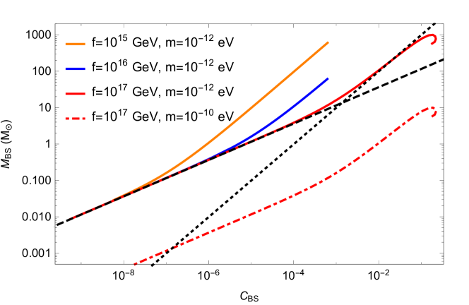
2.4 Linear vs Nonlinear Regime
We notice from Fig. 1 that the stable branch of the boson star admits two regimes where and scale differently. In the linear regime, the boson star mass scales as , while in the nonlinear regime, the scaling goes as . These scalings can be understood as follows. In the non-relativistic limit, the following two parameter ansatz can be taken
| (19) |
The boson star energy is approximated as
| (20) |
In the regime of linear scaling, the gradient (first term) balances with gravity (last term). This leads to , which is
| (21) |
For a fixed compactness, the mass of the boson star is inversely proportional to the scalar mass, ; for a fixed scalar mass, the compactness is proportional to the boson star mass squared, .
In the regime of nonlinear scaling, it is the repulsive term (second term) that balances with gravity (last term) in Eq. (20). This leads to , which indicates
| (22) |
For a given compactness, the star mass is affected by both and , with the relation ; for a given theory point , the mass of the boson star scales with compactness linearly, .
The above behavior in both linear and nonlinear regimes are observed in the numerical solutions, shown in Fig. 1.
3 Extreme Mass Ratio Inspiral and Gravitational Waves
Having obtained the profile of the boson star, we now turn to a calculation of the gravitational waves from EMRI.
3.1 Stellar Dynamics near the SMBH and EMRI
A SMBH resides in the center of most galaxies and its mass ranges from to . Compared with the mass of a typical galaxy hosting it (), the mass of the SMBH is negligibly small. It is only the innermost region of the galaxy, within several parsecs around the SMBH, where the SMBH can have a dominant effect. It is here that an EMRI system can be formed. This region is defined by the radius of influence of the SMBH:
| (23) |
where is the velocity dispersion in the galactic bulge and in the second equality above, the region is used Ferrarese:2000se ; Gebhardt:2000fk ; Tremaine:2002js .
Within the radius of influence, the potential of the SMBH dominates and the total mass of the stellar objects is roughly equal to the mass of the SMBH. Here, the stellar population consists of neutron stars, stellar black holes, white dwarfs(see e.g. Ref. Alexander:2005jz ) and possibly ECOs. This region is very crowded, hence the ECO being within the SMBH influence radius does not guarantee a slow inspiral to be successfully finished. The main physical mechanisms that affect the inspiral of the ECO include two-body relaxation and resonant relaxation. The studies of the dynamics of the stars rely on a phase space analysis (we refer the reader to Ref. alexander:review for a recent review on this subject). As the SMBH devours any compact objects that get sufficiently close to it, there is a loss cone in the phase space. The slow inspiral of EMRI requires that the ECO be sufficiently close to the SMBH so that the time scale for the EMRI to complete is smaller than the typical relaxation time scales and the EMRI can finish without being interrupted by the other stars. It is for this kind of ECO in the slow inspiral phase that an EMRI be formed with gravitational waves detectable by LISA.
3.2 Gravitational Waves
The standard EMRI system consists of a stellar black hole of typical mass and a SMBH of , resulting in a mass ratio that is an extremely small (or large) number. Calculating the waveforms of the EMRI system is a technically challenging and ongoing effort. In Ref. Babak:2017tow , three different waveforms have been used to tackle the data analysis issues for the EMRI systems. This includes the Kludge-family waveforms, which started with the early work of Ref. Barack:2003fp and is now called the Analytical Kludge (AK) model. This has subsequently grown into the numerical AK Babak:2006uv and augmented AK Chua:2017ujo models. Also considered in Ref. Babak:2017tow is the result presented in Ref. Finn:2000sy for circular orbits in the equatorial plane, which is calculated based on the Teukolsky formalism Teukolsky:1973ha ; Sasaki:1981sx . It was found that the results of Ref. Finn:2000sy show overall consistency with the other waveforms. 222The emission of gravitational waves tends to render the orbit of the compact object circular. However astrophysical studies still suggest that the compact object can have significant eccentricity such as through induction Randall:2017jop . We thus assume, for simplicity, that the compact object has a circular orbit in the equatorial plane.
The gravitational wave amplitude is described in terms of the dimensionless characteristic strain, which is decomposed into a set of harmonics labelled by :
| (24) | |||||
where is the mass ratio of boson star () and SMBH (); is the distance to the Earth; is a dimensionless orbital angular frequency where with the Boyer-Lindquist radial coordinates of the orbit; captures the relativistic corrections. 333We use geometrized units here, i.e. and .
Given the above gravitational strain, the detectability of the EMRI gravitational waves signal is quantified by the signal-to-noise ratio (SNR):
| (25) |
which is obtained with matched-filtering Moore:2014lga . We choose as the threshold for detection Babak:2017tow , though a lower value of has also been demonstrated to work Babak:2009cj .
In the above equation, the range of the frequency to be integrated over should be taken as the overlap between the band of the detector and of the signal during the time when the detector is operating. For simplicity, we choose the upper end of the frequency band as the one at the ISCO when the compact object remains intact as it enters the event horizon of the SMBH. Conversely, when tidal disruption happens outside the horizon (to be discussed in the following section) the upper end of the band is chosen to be the frequency at the tidal radius of the compact object. The radius at ISCO for a SMBH with mass and spin has been given in Ref. Bardeen:1972fi .
Another important quantity in our calculations is the time remaining to ISCO. For a given value of the gravitational wave frequency, it is given by Finn:2000sy
| (26) |
where is a general relativistic correction factor, which is a function of the frequency and the SMBH spin. This equation can be reversed to calculate the frequency, given the time remaining to ISCO. For example, setting to be years gives the lower end of the frequency band in the SNR for the fiducial detector of LISA in the case that the compact object enters the horizon intact.
Since the boson star lingers around the ISCO for a very long time, it can travel a large number of cycles around the SMBH. This number is given by Finn:2000sy
| (27) |
where captures the general relativistic correction, similar to the previous quantity . equals one as and vanishes as . A typical value for in LISA band is , much larger than the corresponding quantity in the LIGO case.
Since the SNR is proportional to the square root of Moore:2014lga , it is greatly enhanced for the EMRI system. To phrase this in an illuminating way, LISA will be able to see much further distances.
Moreover, due to the large circle time recorded over several years, the analysis of the gravitational wave waveforms from an EMRI system can lead to a very precise determination of the parameters in the system, such as the masses of the system and the SMBH spin. The uncertainties can be as small as Barack:2003fp . Therefore detection of gravitational waves from an EMRI system where the smaller object has sub-solar mass would definitely rule out the possibility of it being stellar black holes, neutron stars and white dwarfs.
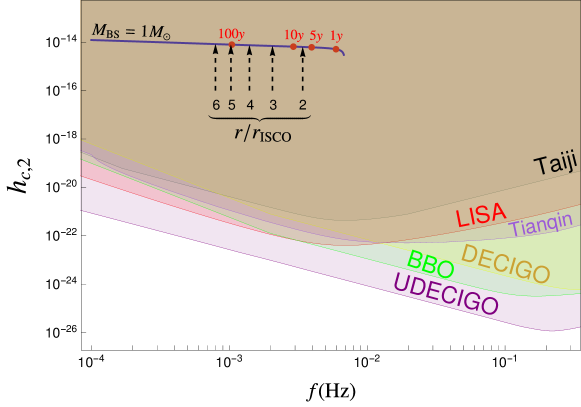
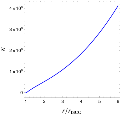
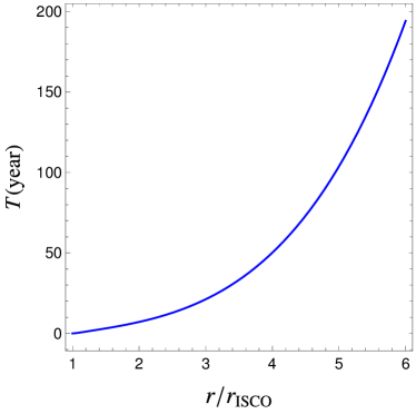
As an example, the solid blue line in Fig. 2 shows the gravitational wave characteristic strain as a function of the frequency for a boson star inspiralling into the SMBH of mass (see caption for more details). The dots on this line denote several time stamps before reaching the ISCO. Also plotted in Fig. 2 are experimental sensitive regions for several proposed detectors, including LISA with configuration C1 Klein:2015hvg , the Taiji Gong:2014mca and Tianqin projects Luo:2015ght , the Big Bang Observer (BBO), the DECi-hertz Interferometer Gravitational wave Observatory (DECIGO) Moore:2014lga , and Ultimate-DECIGO (UDECIGO) Kudoh:2005as . In addition, the number of circles remaining and the time remaining until the ISCO is shown in the left and right panels of Fig. 3 respectively, as a function of . We see that the typical size of the number of circles remaining in the LISA band is indeed very large.
4 Results
In this section, we present our results. We first show the results of our EMRI analysis on the mass versus compactness plane of boson stars. We then discuss the constraints in theory space. We finally comment on the event rate and the possibility of correlated electromagnetic signals.
4.1 Constraints on Mass versus Compactness
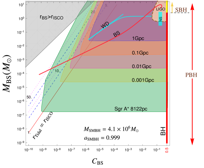
The EMRI analysis described in the previous section leads to strong constraints on the properties of boson stars, which we now describe. Our results are presented in Fig. 4, where we show the regions in the mass versus compactness plane of boson stars that can be probed by LISA and LIGO (see caption for details). Gravitational waves from a boson star binary that can be detected by LIGO are obtained in the upper-right corner, for large mass and compactness. For the LIGO bounds, a distance to Earth larger than Gpc is taken, and the detection threshold of the SNR is assumed to be 8 Dominik:2014yma .
The color-shaded regions in Fig. 4 correspond to an EMRI system emitting gravitational waves with SNR larger than 20 for the LISA detector assuming 5 years of mission time. The EMRI system is composed of a boson star with the corresponding compactness and mass, and a SMBH of mass and spin , the same as that used in Fig. 2. The different colors denote different distance ranges where such detection can be made. The red curve is a representative boson star solution for the parameter choice of and . Also plotted are the regions of white dwarfs (WD), neutron stars (NS) and black holes (BH) (stellar black holes (SBH) by vertical yellow line or primordial black holes (PBH) by vertical red line).
4.2 Tidal Radius
We now turn to a discussion of the tidal radius. For an EMRI system where the small object is a white dwarf, neutron star or primordial black hole, the object is compact enough so that it can generally pass the ISCO without being tidally disrupted, resulting in a gravitational wave signal that lasts until the ISCO. Boson stars, on the other hand, can have compactness well below yet still are detectable at LISA. For a boson star with a fixed mass, decreasing the compactness leads to an increase in the tidal radius. As the tidal radius reaches values greater than the ISCO, the boson star will be tidally disrupted outside the ISCO. The gravitational wave signal will then be cut off at the tidal radius and the maximal frequency recorded by the detector will be smaller than what can be achieved at the ISCO.
We therefore see that for boson stars, the frequency range in the SNR needs to take the tidal disruption into account. Thus for each choice of , we need to find the corresponding tidal radius and compare it with to determine the correct frequency band to be used in the SNR calculations.
For a non-spinning SMBH with mass , the tidal radius can be obtained simply by equating the force of the SMBH at with the self-gravitating force of the BS. This gives the well known result for 444We note that for a Kerr SMBH, a more precise definition of the tidal radius can be found by calculating the general relativistic tidal tensor (see Ref. stone:2015tidal for a review). We leave a more detailed investigation of EMRI with spinning SMBHs for a future publication.:
| (28) |
where in the second step we have traded for . Note that this radius is roughly the same as the Roche radius. Since and , the tidal radius will be inside the horizon for SMBH with mass larger than a threshold, known as the Hill mass stone:2015tidal .
In Fig. 4, several choices of the tidal radius are shown in units of . Since this is a log-log plot, each appears as a straight line. The straight lines show the tidal radius in units of , and the one where coincides with the ISCO is shown by the red line. The gray region in the top left corner gives a boson star radius that is larger than the radius of ISCO.
With determined above, the next step is to find the corresponding frequency at and the associated frequency 5 years before reaching , which is used as the lower limit of the frequency band. Therefore, for the boson stars that experience tidal disruption, the frequency band of the gravitational wave signal is instead of because .
For a Kerr SMBH, the ISCO radius decreases as its spin parameter increases from negative (retrograde motion) to positive values (prograde motion). Therefore, an ECO can in general get closer towards the SMBH for prograde orbits before it reaches the larger of and , compared with the retrograde case whose is larger. Conversely, as the SMBH spin decreases, expands and the condition will be reached for less compact BS when its mass is fixed, which means the boson stars are less likely to get tidally disrupted. This corresponds to that the straight lines in Fig. 4 will shift towards the left.
We need to ensure that the tidal radius is smaller than the radius of influence of the SMBH, so that an EMRI is formed in the first place. This condition is generally straightforward to satisfy for most cases. For example, for a SMBH with mass , the tidal radius needs to be as large as to become comparable to the radius of influence pc. Therefore boson stars that generate gravitational waves within the LISA band are certain to be within the radius of influence. This can be seen in Fig. 4, where the regions of parameter space probed by LISA can only be reached for tidal radius of .
Besides the tidal radius which affects less compact boson stars, other tidal interactions can show up, modifying boson star profiles as well as the resulting gravitational wave waveforms. A boson star can be tidally deformed before it reaches the tidal radius. The deformability can be characterized by the tidal love numbers and has been studied for neutron stars Damour:2009vw and boson stars Cardoso:2017cfl ; Binnington:2009bb . The resulting impact on the gravitational wave waveforms, however, is a secondary effect Barack:2003fp .
The same is true for the spin of the boson star, as well as the spin-orbital coupling effect. Astrophysical studies of the tidal interactions of the stars near the SMBH show that stars can accumulate spins through constantly squeezing at the pericenter. The same is expected to happen for boson stars and a rotating boson star may be formed. Rotating boson star solutions have been considered in Ref. Mielke:2016war 555 The rotating boson star may have a different mass-radius relation compared to the non-rotating case. The main effect is in changing the tidal radius.. However as far as gravitational waves are concerned, these effects tend to be negligible.
We point out that tidal effects in inspiralling binary systems have been studied as a potential discriminant between ordinary compact objects and boson stars Sennett:2017etc .
4.3 Probed Theory Space

Based on the EMRI analysis, the probed region on the mass versus compactness parameter space can now be translated into the theory space . Instead of translating all the probed region to the theory parameter space, we look at a subset where boson stars experience tidal disruption right before reaching . Because the early termination of the inspiral signal gives us extra information about the compactness of the infalling object, we refer such boson stars as distinguishable boson stars.
The distinguishable boson star compactness corresponding to the situation where tidal forces severely disrupt it right before ISCO is given by the line of in Fig. 4. On the other hand, the infalling star needs to be large enough to accumulate enough SNR at LISA. Therefore, for a given luminosity distance, we require the boson star mass profile to be above the intersection point of line and the sensitivity contour, which guarantees a segment of the mass curve falling into the sensitivity region of LISA yet still has an early termination feature. For the top three benchmark contours in Fig. 4, the intersection points correspond to
| (29) | |||||
| (30) | |||||
| (31) |
Requiring the boson star mass profile being above these points leads to the upper limit of the scalar mass in the theory space shown in Fig. 5. In addition, we require the boson star mass curve has a segment such that a) it has overlap with LISA sensitivity region; b) lighter than 1 . This results in the lower bound on the scalar mass that corresponds to the left edge of Fig. 5. We compute the region of transition between linear regime and nonlinear regime numerically to get the solid part of the curves, and invoke the argument in Section 2.4 to compute other regions analytically. The color shaded region show the parameter space that allow for such distinguishable stars.
4.4 Correlated Electromagnetic Signals
We sketch some general ideas about the possibility of obtaining correlated gravitational wave and electromagnetic signals coming from boson star-SMBH EMRIs. Tidal disruption flares coming from ordinary stars near SMBH are an important target in the astrophysics community. We refer to Komossa:2015qya for a review on current observations and Lodato:2015aoa for a review of the theory. Therefore such electromagnetic products coming from the tidal disruption of exotic compact objects is an important and relatively unexplored topic. The signals would depend on the coupling of the boson to Standard Model fields, and one would have to take into account the resulting effects on the boson star profile. While such modeling is outside the scope of our present work, we note that the possibility of unique tidal flares from boson stars would constitute a key piece of observational evidence about their existence.
4.5 Event Rate
The estimation of the event rate of the EMRI from the ECO depends on its population in the radius of influence of the SMBH, which in turn depends on its formation mechanism and how the ECOs sank into the galactic center. Without a prior knowledge of these, an upper limit of the event rate can be set by assuming that the ECOs formed from material that was part of the dark matter halo. While we do not give a solid connection between ECO and dark matter, there have already been many studies of this scenario in the literature Croon:2018ybs . If ECOs indeed form from the dark matter halo, then the event rate for the EMRI from the ECOs can be related to the halo profile.
Here we briefly sketch a few factors that may affect the EMRI event rate. Since EMRI is formed in the galactic center, the event rate of the EMRI depends on the halo density in the innermost parsec region of the galaxy. While collisionless dark matter simulations lead to cuspy NFW profile, dwarf galaxies usually turns out to be cored, due to baryonic feedback Navarro:1996bv ; Pontzen:2011ty , or new physics such as dark matter self-interaction Tulin:2017ara or fuzzy dark matter Schive:2014hza ; Hui:2016ltb . The accuracy in modeling the central density profile Navarro:1995iw ; Navarro:1996gj will affect the estimate of the EMRI event rate. On the other hand, without a good prior on the central density, the measured EMRI event rate could shed light on the environment in the very center of the galaxy. In addition, the presence of the SMBH may lead to a spike of the dark halo Gondolo:1999ef ; Sadeghian:2013laa ; Sandick:2016zeg , which might be further enhanced by the spinning of the SMBH Ferrer:2017xwm . Therefore variations can arise due to the different choices of the halo profiles.
For a given dark matter halo profile, the halo provides an initial ECO population near . Within the radius of influence, the ECOs will be redistributed due to collisions (gravitational encounters) with other stars within the potential well of the SMBH. For a relaxed ECO population, a density cusp can be formed, in analogy to the Bahcall-Wolf stellar cusp gahcall:1976aa . Furthermore, due to the effect of mass segregation Hopman:2006xn ; AmaroSeoane:2010bq ; Alexander:2008tq , heavier ECOs will sink deeper toward the SMBH while lighter ECOs will be pushed outward, leading to an additional enhancement (reduction) of the profile for heavy (light) ECOs at small , respectively. This introduces a dependence of the event rate on ECO mass. If we assume an NFW profile and that the ECO makes up the whole dark halo, then LISA, assuming 5 years of observation time, will be able to see EMRIs for ECOs heavier than (but lighter than so that there is a sufficient number of ECOs for a given halo profile). This estimate is based on a similar analysis for primordial black hole dark matter Guo:2017njn .
5 Summary
In this paper, we have proposed to use gravitational waves from EMRIs as a new method to search for boson stars. We first introduced the particle physics model and computed the profile of the boson star in the mass-compactness plane. The results of numerically solving the Einstein-Klein-Gordon system were displayed in Fig. 1, after which we discussed the linear and nonlinear regimes of the stable branch.
In Section 3, we provided the calculation of the gravitational waves from EMRI. The gravitational wave characteristic strain relevant for us is displayed in Fig. 2. One of the most important features of the EMRI system is that a boson star can linger around the ISCO for a very long time, implying that a large number of cycles around the SMBH are possible. Since the SNR is proportional to , it is greatly enhanced for an EMRI. The number of cycles remaining as a function of the distance from the SMBH, normalized by the ISCO radius, is shown in Fig. 3.
Our main results are presented in Fig. 4, where we show the regions in the mass versus compactness plane of boson stars that can be probed by EMRI at LISA. Clearly, our methods are able to probe boson stars down to very sub-solar mass and compactness. We are careful to incorporate the effect of tidal disruption before the boson star reaches the ISCO; in such cases the signal is cut off at the tidal radius and the maximal frequency recorded by the detector is smaller than what can be achieved at the ISCO.
Due to the large number of cycles recorded, EMRIs can lead to a very precise mass determination of the boson star and distinguish it from standard astrophysical compact objects. From Fig. 4, where standard astrophysical compact objects are also shown, it is clear that a precise determination of the mass of the participating body will distinguish between ECOs and usual compact objects. Tidal effects in inspiralling binary systems further break the mass degeneracy of boson stars with other ECOs candidates. Possible correlated electromagnetic signals, can also serve as potential discriminants.
On the particle physics side, our main results are shown in Fig. 5. We looked into the theory parameter region that admits boson stars in the LISA sensitivity contour yet experience tidal force disruption before reaching . At the same time, we require the boson stars to be lighter than 1 . The result shows a large parameter region where such boson stars are allowed.
There are several future directions to be considered. This work paves the way for future more detailed analysis including improvements on the following sides: consideration of more generic eccentric orbits and using more accurate waveforms, studying changes to the waveform due to tidal deformability of the ECO to distinguish different species of ECOs, dedicated analysis of the tidal disruption events, application to BS with more complicated structures and to other species of ECOs, etc. In addition, when the coupling to the Standard Model particles are taken into account, richer phenomenology is expected, such as electromagnetic signals that accompany the merger events. We leave this for future study.
6 Acknowledgments
We thank Djuna Croon for discussions and JiJi Fan for reading the manuscript. K. Sinha and H. Guo are supported by the U. S. Department of Energy grant DE-SC0009956. C. Sun is supported in part by the International Postdoctoral Fellowship funded by China Postdoctoral Science Foundation, and NASA grant 80NSSC18K1010.
References
- (1) M. Colpi, S. L. Shapiro, and I. Wasserman, “Boson Stars: Gravitational Equilibria of Selfinteracting Scalar Fields,” Phys. Rev. Lett. 57 (1986) 2485–2488.
- (2) I. I. Tkachev, “Coherent scalar field oscillations forming compact astrophysical objects,” Sov. Astron. Lett. 12 (1986) 305–308. [Pisma Astron. Zh.12,726(1986)].
- (3) J. J. van der Bij and M. Gleiser, “Stars of Bosons with Nonminimal Energy Momentum Tensor,” Phys. Lett. B194 (1987) 482–486.
- (4) P. Jetzer, “Boson stars,” Phys. Rept. 220 (Nov., 1992) 163–227.
- (5) F. E. Schunck and E. W. Mielke, “General relativistic boson stars,” Class. Quant. Grav. 20 (2003) R301–R356, arXiv:0801.0307 [astro-ph].
- (6) S. L. Liebling and C. Palenzuela, “Dynamical Boson Stars,” Living Rev. Rel. 15 (2012) 6, arXiv:1202.5809 [gr-qc]. [Living Rev. Rel.20,no.1,5(2017)].
- (7) Virgo, LIGO Scientific Collaboration, B. P. Abbott et al., “Observation of Gravitational Waves from a Binary Black Hole Merger,” Phys. Rev. Lett. 116 no. 6, (2016) 061102, arXiv:1602.03837 [gr-qc].
- (8) M. Gleiser, “Gravitational radiation from primordial solitons and soliton-star binaries,” Physical Review Letters 63 (Sept., 1989) 1199–1202.
- (9) C. Palenzuela, I. Olabarrieta, L. Lehner, and S. L. Liebling, “Head-on collisions of boson stars,” Phys. Rev. D75 (2007) 064005, arXiv:gr-qc/0612067 [gr-qc].
- (10) C. Palenzuela, L. Lehner, and S. L. Liebling, “Orbital Dynamics of Binary Boson Star Systems,” Phys. Rev. D77 (2008) 044036, arXiv:0706.2435 [gr-qc].
- (11) M. A. Amin, E. A. Lim, and I.-S. Yang, “A scattering theory of ultrarelativistic solitons,” Phys. Rev. D88 no. 10, (2013) 105024, arXiv:1308.0606 [hep-th].
- (12) M. Bezares and C. Palenzuela, “Gravitational Waves from Dark Boson Star binary mergers,” Class. Quant. Grav. 35 no. 23, (2018) 234002, arXiv:1808.10732 [gr-qc].
- (13) T. Helfer, E. A. Lim, M. A. G. Garcia, and M. A. Amin, “Gravitational Wave Emission from Collisions of Compact Scalar Solitons,” Phys. Rev. D99 no. 4, (2019) 044046, arXiv:1802.06733 [gr-qc].
- (14) N. Sanchis-Gual, C. Herdeiro, J. A. Font, E. Radu, and F. Di Giovanni, “Head-on collisions and orbital mergers of Proca stars,” Phys. Rev. D99 no. 2, (2019) 024017, arXiv:1806.07779 [gr-qc].
- (15) D. Croon, J. Fan, and C. Sun, “Boson Star from Repulsive Light Scalars and Gravitational Waves,” arXiv:1810.01420 [hep-ph].
- (16) D. Croon, M. Gleiser, S. Mohapatra, and C. Sun, “Gravitational Radiation Background from Boson Star Binaries,” Phys. Lett. B783 (2018) 158–162, arXiv:1802.08259 [hep-ph].
- (17) G. F. Giudice, M. McCullough, and A. Urbano, “Hunting for Dark Particles with Gravitational Waves,” JCAP 1610 no. 10, (2016) 001, arXiv:1605.01209 [hep-ph].
- (18) L. Barack and C. Cutler, “LISA capture sources: Approximate waveforms, signal-to-noise ratios, and parameter estimation accuracy,” Phys. Rev. D69 (2004) 082005, arXiv:gr-qc/0310125 [gr-qc].
- (19) A. Klein et al., “Science with the space-based interferometer eLISA: Supermassive black hole binaries,” Phys. Rev. D93 no. 2, (2016) 024003, arXiv:1511.05581 [gr-qc].
- (20) R. Ruffini and S. Bonazzola, “Systems of selfgravitating particles in general relativity and the concept of an equation of state,” Phys. Rev. 187 (1969) 1767–1783.
- (21) D. G. Levkov, A. G. Panin, and I. I. Tkachev, “Relativistic axions from collapsing Bose stars,” Phys. Rev. Lett. 118 no. 1, (2017) 011301, arXiv:1609.03611 [astro-ph.CO].
- (22) M. Gleiser and R. Watkins, “Gravitational Stability of Scalar Matter,” Nucl. Phys. B319 (1989) 733–746.
- (23) M. Gleiser and D. Sicilia, “A General Theory of Oscillon Dynamics,” Phys. Rev. D80 (2009) 125037, arXiv:0910.5922 [hep-th].
- (24) J. Eby, P. Suranyi, and L. C. R. Wijewardhana, “The Lifetime of Axion Stars,” Mod. Phys. Lett. A31 no. 15, (2016) 1650090, arXiv:1512.01709 [hep-ph].
- (25) J. Eby, P. Suranyi, and L. C. R. Wijewardhana, “Expansion in Higher Harmonics of Boson Stars using a Generalized Ruffini-Bonazzola Approach, Part 1: Bound States,” JCAP 1804 no. 04, (2018) 038, arXiv:1712.04941 [hep-ph].
- (26) L. Visinelli, S. Baum, J. Redondo, K. Freese, and F. Wilczek, “Dilute and dense axion stars,” Phys. Lett. B777 (2018) 64–72, arXiv:1710.08910 [astro-ph.CO].
- (27) M. P. Hertzberg and E. D. Schiappacasse, “Dark Matter Axion Clump Resonance of Photons,” JCAP 1811 no. 11, (2018) 004, arXiv:1805.00430 [hep-ph].
- (28) S. H. Hawley and M. W. Choptuik, “Boson stars driven to the brink of black hole formation,” Phys. Rev. D62 (2000) 104024, arXiv:gr-qc/0007039 [gr-qc].
- (29) E. Braaten, A. Mohapatra, and H. Zhang, “Dense Axion Stars,” Phys. Rev. Lett. 117 no. 12, (2016) 121801, arXiv:1512.00108 [hep-ph].
- (30) E. D. Schiappacasse and M. P. Hertzberg, “Analysis of Dark Matter Axion Clumps with Spherical Symmetry,” JCAP 1801 (2018) 037, arXiv:1710.04729 [hep-ph]. [Erratum: JCAP1803,no.03,E01(2018)].
- (31) P.-H. Chavanis, “Phase transitions between dilute and dense axion stars,” Phys. Rev. D98 no. 2, (2018) 023009, arXiv:1710.06268 [gr-qc].
- (32) J. Fan, “Ultralight Repulsive Dark Matter and BEC,” Phys. Dark Univ. 14 (2016) 84–94, arXiv:1603.06580 [hep-ph].
- (33) L. Ferrarese and D. Merritt, “A Fundamental relation between supermassive black holes and their host galaxies,” Astrophys. J. 539 (2000) L9, arXiv:astro-ph/0006053 [astro-ph].
- (34) K. Gebhardt et al., “A Relationship between nuclear black hole mass and galaxy velocity dispersion,” Astrophys. J. 539 (2000) L13, arXiv:astro-ph/0006289 [astro-ph].
- (35) S. Tremaine et al., “The slope of the black hole mass versus velocity dispersion correlation,” Astrophys. J. 574 (2002) 740–753, arXiv:astro-ph/0203468 [astro-ph].
- (36) T. Alexander, “Stellar processes near the massive black hole in the Galactic Center,” Phys. Rept. 419 (2005) 65–142, arXiv:astro-ph/0508106 [astro-ph].
- (37) T. Alexander, “Stellar dynamics and stellar phenomena near a massive black hole,” Annual Review of Astronomy and Astrophysics 55 no. 1, (2017) 17–57, https://doi.org/10.1146/annurev-astro-091916-055306. https://doi.org/10.1146/annurev-astro-091916-055306.
- (38) S. Babak, J. Gair, A. Sesana, E. Barausse, C. F. Sopuerta, C. P. L. Berry, E. Berti, P. Amaro-Seoane, A. Petiteau, and A. Klein, “Science with the space-based interferometer LISA. V: Extreme mass-ratio inspirals,” arXiv:1703.09722 [gr-qc].
- (39) S. Babak, H. Fang, J. R. Gair, K. Glampedakis, and S. A. Hughes, “’Kludge’ gravitational waveforms for a test-body orbiting a Kerr black hole,” Phys. Rev. D75 (2007) 024005, arXiv:gr-qc/0607007 [gr-qc]. [Erratum: Phys. Rev.D77,04990(2008)].
- (40) A. J. K. Chua, C. J. Moore, and J. R. Gair, “Augmented kludge waveforms for detecting extreme-mass-ratio inspirals,” Phys. Rev. D96 no. 4, (2017) 044005, arXiv:1705.04259 [gr-qc].
- (41) L. S. Finn and K. S. Thorne, “Gravitational waves from a compact star in a circular, inspiral orbit, in the equatorial plane of a massive, spinning black hole, as observed by LISA,” Phys. Rev. D62 (2000) 124021, arXiv:gr-qc/0007074 [gr-qc].
- (42) S. A. Teukolsky, “Perturbations of a rotating black hole. 1. Fundamental equations for gravitational electromagnetic and neutrino field perturbations,” Astrophys. J. 185 (1973) 635–647.
- (43) M. Sasaki and T. Nakamura, “Gravitational Radiation From a Kerr Black Hole. 1. Formulation and a Method for Numerical Analysis,” Prog. Theor. Phys. 67 (1982) 1788.
- (44) L. Randall and Z.-Z. Xianyu, “Induced Ellipticity for Inspiraling Binary Systems,” Astrophys. J. 853 no. 1, (2018) 93, arXiv:1708.08569 [gr-qc].
- (45) C. J. Moore, R. H. Cole, and C. P. L. Berry, “Gravitational-wave sensitivity curves,” Class. Quant. Grav. 32 no. 1, (2015) 015014, arXiv:1408.0740 [gr-qc].
- (46) Mock LISA Data Challenge Task Force Collaboration, S. Babak et al., “The Mock LISA Data Challenges: From Challenge 3 to Challenge 4,” Class. Quant. Grav. 27 (2010) 084009, arXiv:0912.0548 [gr-qc].
- (47) J. M. Bardeen, W. H. Press, and S. A. Teukolsky, “Rotating black holes: Locally nonrotating frames, energy extraction, and scalar synchrotron radiation,” Astrophys. J. 178 (1972) 347.
- (48) X. Gong et al., “Descope of the ALIA mission,” J. Phys. Conf. Ser. 610 no. 1, (2015) 012011, arXiv:1410.7296 [gr-qc].
- (49) TianQin Collaboration, J. Luo et al., “TianQin: a space-borne gravitational wave detector,” Class. Quant. Grav. 33 no. 3, (2016) 035010, arXiv:1512.02076 [astro-ph.IM].
- (50) H. Kudoh, A. Taruya, T. Hiramatsu, and Y. Himemoto, “Detecting a gravitational-wave background with next-generation space interferometers,” Phys. Rev. D73 (2006) 064006, arXiv:gr-qc/0511145 [gr-qc].
- (51) M. Dominik, E. Berti, R. O’Shaughnessy, I. Mandel, K. Belczynski, C. Fryer, D. E. Holz, T. Bulik, and F. Pannarale, “Double Compact Objects III: Gravitational Wave Detection Rates,” Astrophys. J. 806 no. 2, (2015) 263, arXiv:1405.7016 [astro-ph.HE].
- (52) N. C. Stone, “The Tidal Disruption of Stars by Supermassive Black Holes,” Springer Theses (2015) 1–162.
- (53) T. Damour and A. Nagar, “Relativistic tidal properties of neutron stars,” Phys. Rev. D80 (2009) 084035, arXiv:0906.0096 [gr-qc].
- (54) V. Cardoso, E. Franzin, A. Maselli, P. Pani, and G. Raposo, “Testing strong-field gravity with tidal Love numbers,” Phys. Rev. D95 no. 8, (2017) 084014, arXiv:1701.01116 [gr-qc]. [Addendum: Phys. Rev.D95,no.8,089901(2017)].
- (55) T. Binnington and E. Poisson, “Relativistic theory of tidal Love numbers,” Phys. Rev. D80 (2009) 084018, arXiv:0906.1366 [gr-qc].
- (56) E. W. Mielke, “Rotating Boson Stars,” Fundam. Theor. Phys. 183 (2016) 115–131.
- (57) N. Sennett, T. Hinderer, J. Steinhoff, A. Buonanno, and S. Ossokine, “Distinguishing Boson Stars from Black Holes and Neutron Stars from Tidal Interactions in Inspiraling Binary Systems,” Phys. Rev. D96 no. 2, (2017) 024002, arXiv:1704.08651 [gr-qc].
- (58) S. Komossa, “Tidal disruption of stars by supermassive black holes: Status of observations,” JHEAp 7 (2015) 148–157, arXiv:1505.01093 [astro-ph.HE].
- (59) G. Lodato, A. Franchini, C. Bonnerot, and E. M. Rossi, “Recent developments in the theory of tidal disruption events,” JHEAp 7 (2015) 158–162.
- (60) J. F. Navarro, V. R. Eke, and C. S. Frenk, “The cores of dwarf galaxy halos,” Mon. Not. Roy. Astron. Soc. 283 (1996) L72–L78, arXiv:astro-ph/9610187 [astro-ph].
- (61) A. Pontzen and F. Governato, “How supernova feedback turns dark matter cusps into cores,” Mon. Not. Roy. Astron. Soc. 421 (2012) 3464, arXiv:1106.0499 [astro-ph.CO].
- (62) S. Tulin and H.-B. Yu, “Dark Matter Self-interactions and Small Scale Structure,” arXiv:1705.02358 [hep-ph].
- (63) H.-Y. Schive, M.-H. Liao, T.-P. Woo, S.-K. Wong, T. Chiueh, T. Broadhurst, and W. Y. P. Hwang, “Understanding the Core-Halo Relation of Quantum Wave Dark Matter from 3D Simulations,” Phys. Rev. Lett. 113 no. 26, (2014) 261302, arXiv:1407.7762 [astro-ph.GA].
- (64) L. Hui, J. P. Ostriker, S. Tremaine, and E. Witten, “Ultralight scalars as cosmological dark matter,” Phys. Rev. D95 no. 4, (2017) 043541, arXiv:1610.08297 [astro-ph.CO].
- (65) J. F. Navarro, C. S. Frenk, and S. D. M. White, “The Structure of cold dark matter halos,” Astrophys. J. 462 (1996) 563–575, arXiv:astro-ph/9508025 [astro-ph].
- (66) J. F. Navarro, C. S. Frenk, and S. D. M. White, “A Universal density profile from hierarchical clustering,” Astrophys. J. 490 (1997) 493–508, arXiv:astro-ph/9611107 [astro-ph].
- (67) P. Gondolo and J. Silk, “Dark matter annihilation at the galactic center,” Phys. Rev. Lett. 83 (1999) 1719–1722, arXiv:astro-ph/9906391 [astro-ph].
- (68) L. Sadeghian, F. Ferrer, and C. M. Will, “Dark matter distributions around massive black holes: A general relativistic analysis,” Phys. Rev. D88 no. 6, (2013) 063522, arXiv:1305.2619 [astro-ph.GA].
- (69) P. Sandick, K. Sinha, and T. Yamamoto, “Black Holes, Dark Matter Spikes, and Constraints on Simplified Models with -Channel Mediators,” Phys. Rev. D98 no. 3, (2018) 035004, arXiv:1701.00067 [hep-ph].
- (70) F. Ferrer, A. M. da Rosa, and C. M. Will, “Dark matter spikes in the vicinity of Kerr black holes,” arXiv:1707.06302 [astro-ph.CO].
- (71) J. N. Bahcall and R. A. Wolf, “Star distribution around a massive black hole in a globular cluster,” Astrophys. J. 209 (1976) 214–232.
- (72) C. Hopman and T. Alexander, “The effect of mass-segregation on gravitational wave sources near massive black holes,” Astrophys. J. 645 (2006) L133–L136, arXiv:astro-ph/0603324 [astro-ph].
- (73) P. Amaro-Seoane and M. Preto, “The impact of realistic models of mass segregation on the event rate of extreme-mass ratio inspirals and cusp re-growth,” Class. Quant. Grav. 28 (2011) 094017, arXiv:1010.5781 [astro-ph.CO].
- (74) T. Alexander and C. Hopman, “Strong mass segregation around a massive black hole,” Astrophys. J. 697 (2009) 1861–1869, arXiv:0808.3150 [astro-ph].
- (75) H.-K. Guo, J. Shu, and Y. Zhao, “Using LISA-like Gravitational Wave Detectors to Search for Primordial Black Holes,” Phys. Rev. D99 no. 2, (2019) 023001, arXiv:1709.03500 [astro-ph.CO].