Imprint of a scalar era on the primordial spectrum of gravitational waves

Abstract

Upcoming searches for the stochastic background of inflationary gravitational waves (GWs) offer the exciting possibility to probe the evolution of our Universe prior to Big Bang nucleosynthesis. In this spirit, we explore the sensitivity of future GW observations to a broad class of beyond-the-Standard-Model scenarios that lead to a nonstandard expansion history. We consider a new scalar field whose coherent oscillations dominate the energy density of the Universe at very early times, resulting in a scalar era prior to the standard radiation-dominated era. The imprint of this scalar era on the primordial GW spectrum provides a means to probe well-motivated yet elusive models of particle physics. Our work highlights the complementarity of future GW observatories across the entire range of accessible frequencies.

Introduction. The detection of gravitational waves (GWs) Abbott:2016blz by LIGO Harry:2010zz ; TheLIGOScientific:2014jea and Virgo TheVirgo:2014hva has rung in the age of GW astronomy. While all signals observed thus far have been of astrophysical origin, i.e., the coalescence of compact binaries LIGOScientific:2018mvr , it is expected that GWs will also open a window on cosmology in the foreseeable future Maggiore:1999vm . Within the next decades, a multitude of GW observatories will go online, ranging from third-generation ground-based interferometers over satellite-borne interferometers in space to pulsar timing arrays monitored by new radio telescopes (see McWilliams:2019fng ; Caldwell:2019vru ; Kalogera:2019sui ; Cornish:2019fee ; LIGOScientific:2019vkc for an outlook on GW astronomy in the 2020’s). These experiments promise to be sensitive to a wealth of hypothetical cosmological GW signals — such as the stochastic GW background (SGWB) from inflation, GWs from phase transitions in the early Universe, or GWs emitted by topological defects (see Caprini:2018mtu ; Christensen:2018iqi for recent review articles) — and even to anisotropies in the GW signal Geller:2018mwu . The direct observation of any of these cosmological signals would allow one to chart unexplored territory that cannot be accessed by conventional cosmological probes such as the cosmic microwave background (CMB) or the primordial abundances of light elements generated during Big Bang nucleosynthesis (BBN).

In this paper, we will be concerned with the primordial SGWB from inflation Grishchuk:1974ny ; Starobinsky:1979ty ; Rubakov:1982df (see Guzzetti:2016mkm for a review). An intriguing feature of inflationary GWs is that they act as a logbook of the expansion history of our Universe throughout its evolution Seto:2003kc ; Boyle:2005se ; Boyle:2007zx ; Kuroyanagi:2008ye ; Nakayama:2009ce ; Kuroyanagi:2013ns ; Jinno:2013xqa ; Saikawa:2018rcs . Indeed, the detailed time evolution of the Hubble rate during the expansion determines the transfer function that describes how gravitational waves at different frequencies are redshifted to the present day. This property turns primordial GWs into a powerful tool that grants access to the thermal history of our Universe prior to BBN. Primordial GWs offer, e.g., an opportunity to measure the reheating temperature after inflation Nakayama:2008ip ; Nakayama:2008wy ; Kuroyanagi:2011fy ; Buchmuller:2013lra ; Buchmuller:2013dja ; Jinno:2014qka ; Kuroyanagi:2014qza . Similarly, they may be used to infer the equation of state (EOS) during the quark-hadron phase transition in quantum chromodynamics Schettler:2010dp ; Hajkarim:2019csy or constrain properties of hidden sectors beyond the Standard Model (BSM) Jinno:2012xb ; Caldwell:2018giq . The same may also be true for GWs emitted by cosmic strings Cui:2017ufi ; Cui:2018rwi , whose detailed properties are currently under discussion (see Matsui:2019obe and references therein).

The main goal of this paper is to demonstrate how future observations of the primordial SGWB from inflation across a large range of frequencies will be instrumental in constraining BSM physics. To this end, we shall consider a broad class of new physics models in which the presence of a scalar field $\phi$ in the early Universe leads to a modified expansion history. Such a situation can occur in a variety of BSM scenarios. Possible BSM scalar fields that $\phi$ may be identified as include, but are not limited to: the Polonyi field in models of gravity-mediated supersymmetry breaking Coughlan:1983ci ; Ellis:1986zt , a modulus field in four-dimensional compactifications of string theory deCarlos:1993wie ; Moroi:1999zb ; Durrer:2011bi ; Kane:2015jia , a flavon field in extensions of the Standard Model (SM) that aim at explaining the flavor structure of quark and leptons (such as, e.g., the Froggatt-Nielsen flavor model Froggatt:1978nt ), and the saxion field in supersymmetric axion models Kugo:1983ma ; Banks:2002sd ; Kawasaki:2008jc ; Harigaya:2013vja ; Harigaya:2015soa ; Co:2016vsi ; Co:2017orl .

At some point prior to BBN, the energy density stored in the coherent oscillations of the scalar field begins to dominate over radiation. The ensuing era of scalar-field domination (SD), or scalar era for short, leads to a characteristic feature in the transfer function for primordial GWs, which may be detected by future GW experiments. In a detailed numerical analysis, we calculate the transfer function for primordial GWs that captures the modified expansion during the scalar era. This allows us to determine the final GW spectrum across the entire relevant parameter space of our scalar-field model. For each parameter point, we compute the signal-to-noise ratios (SNRs) at which the GW spectrum as well as individual features in this spectrum are expected to be observed by various future GW experiments. The outcome of our analysis is a global picture of the GW signature of the scalar era and the experimental prospects of detecting it. Our study highlights the complementarity of future GW experiments across the entire range of accessible frequencies and defines an important benchmark scenario for the experimental GW community in the coming decades.

Primordial gravitational waves. GWs correspond to spatial tensor perturbations $h_{ij}$ of the spacetime metric,

$$ds^{2}=-dt^{2}+a^{2}\left(t\right)\left[\delta_{ij}+h_{ij}\left(t,\mathbf{x}\right)\right]dx^{i}dx^{j}\,,$$ (1)

where $a$ denotes the cosmic scale factor and the symmetric tensor $h_{ij}$ is evaluated in transverse-traceless gauge, $h_{ii}=\partial_{i}\,h_{ij}=0$. The free propagation of GWs is governed by the linearized Einstein equation with a vanishing source term. In Fourier space, one thus obtains the following equations of motion for the tensor modes $h_{\mathbf{k}}^{p}$,

$$\left[\frac{d^{2}}{du^{2}}+\frac{2}{a\left(u\right)}\frac{da\left(u\right)}{du}\frac{d}{du}+1\right]h_{\mathbf{k}}^{p}\left(u\right)=0\,.$$ (2)

Here, $\mathbf{k}$ denotes the comoving 3-momentum with absolute value $k=\left\lVert\mathbf{k}\right\rVert$, $p=+,\times$ distinguishes the two possible polarization states of a GW, and the variable $u=k\tau$ (with $\tau$ denoting conformal time, $dt=a\,d\tau$) is a measure for the spatial extent of a GW. For $u\ll 1$ ($u\gg 1$), a mode is located far outside (inside) the Hubble horizon.

An important property of inflationary GWs is that they are stretched to super-horizon size during inflation. Outside the horizon, GWs remain frozen, until they re-enter the horizon during the decelerating expansion after inflation. This enables one to factorize the amplitude of a GW mode at the present time $\tau_{0}$, $h_{\mathbf{k}}^{p}\left(\tau_{0}\right)=\bar{h}_{\mathbf{k}}^{p}\,\chi_{k}\left(\bar{\tau},\tau_{0}\right)$, into an initial value at $\bar{\tau}$ determined by inflation, $\bar{h}_{\mathbf{k}}^{p}=h_{\mathbf{k}}^{p}\left(\bar{\tau}\right)$, and a transfer function $\chi_{k}\left(\bar{\tau},\tau_{0}\right)$ that accounts for the redshift subsequent to horizon re-entry. For any expansion history after inflation [specified by the function $a\left(u\right)$], the transfer function can be found by solving Eq. (2) for $\chi_{k}$ as a function of $u$ with boundary conditions $\chi_{k}=1$ and $\partial_{u}\chi_{k}=0$ at $u=0$. The same factorization also carries over to $\Omega_{\rm GW}\left(f\right)$, i.e., the GW energy density per logarithmic frequency interval $d\left(\ln f\right)$ in units of the critical energy density of a flat universe. For modes deep inside the horizon, one obtains the following GW spectrum at the present time,

$$\Omega_{\rm GW}^{0}\left(f\right)\simeq\frac{1}{12}\frac{k^{2}}{a_{0}^{2}H_{0}^{2}}\,\mathcal{P}_{t}\left(k\right)\left|\chi_{k}\right|^{2}\,,\quad f=\frac{k}{2\pi\,a_{0}}\,,$$ (3)

where $a_{0}$ and $H_{0}=100\,h\,\textrm{km}/\textrm{s}/\textrm{Mpc}$ represent the present values of the scale factor and the Hubble rate, respectively. The primordial tensor spectrum $\mathcal{P}_{t}$ depends on the initial conditions set by the inflationary period and is conventionally parametrized by a simple power law around the CMB pivot scale, $k_{\rm CMB}=0.05\,\textrm{Mpc}^{-1}$,

$$\mathcal{P}_{t}=\frac{k^{3}}{\pi^{2}}\left(\left|\bar{h}_{\mathbf{k}}^{+}\right|^{2}+\left|\bar{h}_{\mathbf{k}}^{\times}\right|^{2}\right)=A_{t}\left(\frac{k}{k_{\rm CMB}}\right)^{n_{t}}\,.$$ (4)

In this paper, we are interested in assessing the maximal reach of future GW experiments. For this reason, we decide to fix the primordial tensor amplitude at the maximally allowed value, $A_{t}\simeq 1.5\times 10^{-10}$, that is consistent with the most recent upper bound on the tensor-to-scalar ratio, $r=A_{t}/A_{s}\lesssim 0.07$ Akrami:2018odb , where $A_{s}\simeq 2.1\times 10^{-9}$ is the measured amplitude of the primordial scalar spectrum. Similarly, we shall assume a blue-tilted tensor spectrum, fixing its index at an optimistic value of $n_{t}=0.4$. On the one hand, this value clearly violates the consistency relation of standard single-field slow-roll inflation, $n_{t}=-r/8<0$. This means that we implicitly assume a nonminimal inflationary sector that is capable of generating a strong SGWB at small scales. Such scenarios exist in the literature, with one prominent example being natural inflation coupled to gauge fields Cook:2011hg ; Barnaby:2011qe ; Anber:2012du ; Domcke:2016bkh ; Jimenez:2017cdr ; Papageorgiou:2019ecb . On the other hand, our choice for the spectral index is phenomenologically still completely viable. $n_{t}=0.4$ complies with (1) the CMB constraints derived by the PLANCK Collaboration Akrami:2018odb , (2) the upper bound on the amplitude of an isotropic SGWB at $\mathcal{O}\left(10\right)\,\textrm{Hz}$ frequencies by LIGO and Virgo TheLIGOScientific:2016dpb ; LIGOScientific:2019vic , and (3) global bounds on primordial GWs (based, e.g., on BBN) across the full frequency spectrum Kuroyanagi:2014nba ; Lasky:2015lej .

The scalar era. We consider the dynamics of a real scalar field $\phi$, employing an effective description in terms of three parameters: mass $m_{\phi}$, decay rate $\Gamma_{\phi}$, and initial field value $\phi_{\rm ini}$ at the end of inflation. We assume a harmonic potential around the origin in field space and some (direct or indirect) coupling to the Standard Model that allows $\phi$ to decay to radiation at the end of its lifetime. The dynamical evolution of the field $\phi$ is governed by the Klein-Gordon equation in an expanding background,

$$\left[\frac{d^{2}}{dt^{2}}+\left(3\,H\left(t\right)+\Gamma_{\phi}\right)\frac{d}{dt}+m_{\phi}^{2}\right]\phi\left(t\right)=0\,,$$ (5)

where we included a friction term proportional to $\Gamma_{\phi}$. The Hubble rate $H$ follows from the Friedmann equation,

$$H^{2}\left(t\right)=\left[\frac{\dot{a}\left(t\right)}{a\left(t\right)}\right]^{2}=\frac{\rho_{\phi}\left(t\right)+\rho_{R}\left(t\right)}{3\,M_{\rm Pl}^{2}}\,,$$ (6)

where $M_{\rm Pl}\simeq 2.44\times 10^{18}\,\textrm{GeV}$ is the reduced Planck mass and $\rho_{\phi}=1/2\,\dot{\phi}^{2}+1/2\,m_{\phi}^{2}\,\phi^{2}$ denotes the energy density stored in the field $\phi$. The energy density of radiation, $\rho_{R}$, is described by an evolution equation that follows from covariant energy conservation in an expanding universe,

$$\left[\frac{d}{dt}+4\,\frac{g_{*,s}\left(\rho_{R}\left(t\right)\right)}{g_{*,\rho}\left(\rho_{R}\left(t\right)\right)}\,H\left(t\right)\right]\rho_{R}\left(t\right)=\Gamma_{\phi}\,\dot{\phi}^{2}\left(t\right)\,,$$ (7)

Here, $g_{*,s}$ and $g_{*,\rho}$ are the effective numbers of relativistic degrees of freedom that contribute to the entropy and energy densities of radiation, respectively. We will evaluate $g_{*,s}$ and $g_{*,\rho}$ using the numerical data tabulated in Saikawa:2018rcs .

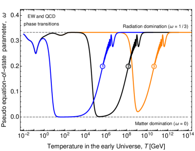
Figure 1: Pseudo EOS parameter $\omega=2/\left(3\,tH\right)-1$ as a function of temperature $T$ for three parameter examples (see Fig. 3). $\omega$ is defined such that $a\propto t^{\alpha}$, where $\alpha=2/3/\left(1+\omega\right)$. It equals the EOS parameter $w=p/\rho$ as long as $w=\textrm{const}$.

Let us now discuss the system of equations (5) to (7). First, we observe that $\phi$ only begins to roll — and eventually oscillate around the origin in field space — once the Hubble rate has dropped below the scalar mass, $H\lesssim m_{\phi}$. At earlier times, the Hubble friction term in (5) keeps $\phi$ more or less fixed at $\phi_{\rm ini}$. For a sufficiently high reheating temperature after inflation, the expansion is initially driven by radiation. $\rho_{R}$ is, however, rapidly redshifted, $\rho_{R}\propto 1/a^{4}$, such that, at some temperature $T_{\rm SD}$, the energy density $\rho_{\phi}$ begins to dominate the expansion,

$$T_{\rm SD}\simeq\frac{b^{2}}{\alpha_{\rm SD}^{3/2}}\left(\frac{5}{36\pi^{2}\,g_{*,\rho}^{\rm SD}}\right)^{1/4}\left(\frac{\phi_{\rm ini}}{M_{\rm Pl}}\right)^{2}\left(m_{\phi}\,M_{\rm Pl}\right)^{1/2}.$$ (8)

Here, $b=\Gamma\left(5/4\right)/\Gamma\left(3/2\right)\simeq 1.02$ stems from the analytic solution of (5) in a radiation-dominated (RD) background, while $\alpha_{\rm SD}\approx 2/3$ characterizes the behavior of the scale factor at the onset of scalar-field domination, $a\left(t\right)\propto t^{\alpha_{\rm SD}}$. The result in (8) is only valid for $\phi_{\rm ini}\lesssim M_{\rm Pl}$. Otherwise, the scalar field has not yet begun to oscillate at the onset of the scalar era, which leads to a short period of vacuum domination. Such a second phase of inflation results in a nontrivial oscillatory feature in the transfer function Jinno:2013xqa . On the other hand, it also causes a stronger dilution of the primordial SGWB, which weakens the expected GW signal. For this reason, we will not consider the case $\phi_{\rm ini}\gtrsim M_{\rm Pl}$ in this work.

After many oscillations around the potential minimum, $t\gg 1/m_{\phi}$, the energy density of the scalar field behaves like the energy density of pressureless dust, $\rho_{\phi}\propto 1/a^{3}$. The scalar era therefore effectively mimics, at least for some intermediate period, a phase of matter-dominated expansion (see Fig. 1). It lasts until $\phi$ decays into SM radiation around $t_{\rm RD}\simeq c/\Gamma_{\phi}$, which marks the onset of the final radiation-dominated era at temperature $T_{\rm RD}$,

$$T_{\rm RD}=\bigg{(}\frac{\alpha_{\rm RD}}{c}\bigg{)}^{1/2}\left(\frac{90}{2\pi^{2}\,g_{*,\rho}^{\rm RD}}\right)^{1/4}\left(\Gamma_{\phi}\,M_{\rm Pl}\right)^{1/2}\,,$$ (9)

where $\alpha_{\rm RD}\approx 2/3$. Assuming a constant EOS throughout the scalar era, one is able to analytically derive $c\simeq 1.07$.

The nonstandard EOS and the late-time entropy injection during the scalar era result in the dilution of sub-horizon tensor modes. This effect is captured by the dilution factor $D=\left[S\left(T\gg T_{\rm SD}\right)/S\left(T\ll T_{\rm RD}\right)\right]^{1/3}$, where $S$ denotes the comoving entropy density, $S=a^{3}\,s$,

$$D=e^{c/3}\,d\,\bigg{(}\frac{g_{*,s}^{\rm SD}}{g_{*,s}^{\rm RD}}\bigg{)}^{1/3}\bigg{(}\frac{g_{*,\rho}^{\rm RD}}{g_{*,\rho}^{\rm SD}}\bigg{)}^{1/4}\eta^{1/6}\,.$$ (10)

The factor $d\simeq 0.80$, which needs to be determined numerically, accounts for entropy production at $T<T_{\rm RD}$. The factor $\eta$ is defined as the ratio of the two values of the Hubble rate at $T=T_{\rm RD}$ and $T=T_{\rm SD}$, respectively,

$$\eta=\frac{H_{\rm RD}}{H_{\rm SD}}=\frac{18\,\alpha_{\rm SD}^{3}\,\alpha_{\rm RD}}{b^{4}\,c}\frac{\Gamma_{\phi}}{m_{\phi}}\left(\frac{M_{\rm Pl}}{\phi_{\rm ini}}\right)^{4}\,.$$ (11)

The two temperatures $T_{\rm SD}$ and $T_{\rm RD}$ also single out two frequencies in the GW spectrum, $f_{\rm SD}$ and $f_{\rm RD}$, which correspond to the tensor modes that re-enter the horizon at these temperatures, respectively. For $f_{\rm RD}$, we find

$$\frac{f_{\rm RD}}{f_{0}}=d\,\bigg{(}\frac{g_{*,s}^{0}}{g_{*,s}^{\rm RD}}\bigg{)}^{1/3}\bigg{(}\frac{g_{*,\rho}^{\rm RD}}{g_{*,\rho}^{0}}\bigg{)}^{1/2}\left(\frac{\Omega_{R}^{0}}{1/2}\right)^{1/2}\frac{T_{\rm RD}}{T_{0}}\,,$$ (12)

where $T_{0}\simeq 2.72548\,\textrm{K}\simeq 2.3\times 10^{-13}\,\textrm{GeV}$ is the current temperature of the CMB Fixsen:2009ug , $h^{2}\Omega_{R}^{0}\simeq 4.2\times 10^{-5}$ denotes the energy density parameter of radiation at the present time, and $f_{0}=H_{0}/\left(2\pi\right)$ corresponds to the frequency of the GW mode that currently stretches across one Hubble radius, $f_{0}/h\simeq 5.2\times 10^{-19}\,\textrm{Hz}$. The frequency $f_{\rm SD}$ can be computed in terms of the quantities in (11) and (12),

$$f_{\rm SD}=\left(\frac{e^{c}}{\eta}\right)^{1/3}f_{\rm RD}\,.$$ (13)

This shows that the parameter $\eta$ determines the duration of the scalar era in frequency space. In our numerical analysis, we will scan over different values of $\eta$ by varying the ratio $m_{\phi}/\Gamma_{\phi}$, while keeping the initial field value fixed at $\phi_{\rm ini}=10^{18}\,\textrm{GeV}$. This benchmark represents a typical value that can be realized in many models as an initial condition after inflation Bunch:1978yq ; Linde:1982uu ; Affleck:1984fy ; Starobinsky:1994bd . Aside from that, it is important to note that, to first approximation, it is straightforward to generalize our analysis to different values of $\phi_{\rm ini}$ by simply rescaling all values of $m_{\phi}/\Gamma_{\phi}$.

Transfer function. For a mode with wave number $k$ deep inside the horizon, the transfer function roughly scales like $\chi_{k}\sim a_{k}/a_{0}$, where $a_{k}$ is the scale factor at the time of horizon re-entry, implicitly defined by $a_{k}=k/H\left(a_{k}\right)$ Turner:1993vb ; Boyle:2005se ; Watanabe:2006qe . For an EOS $w=p/\rho=\textrm{const}$ (with pressure $p$ and energy density $\rho$), this results in a simple power-law scaling of the final GW spectrum,

$$\Omega_{\rm GW}^{0}\left(f\right)\propto f^{n}\,,\quad n=n_{t}+\frac{2\left(3\,w-1\right)}{3\,w+1}\,,$$ (14)

which illustrates the main impact of the scalar era on the GW spectrum: For frequencies $f_{\rm RD}\lesssim f\lesssim f_{\rm SD}$, the spectral index $n$ changes by $\Delta n\simeq-2$ compared to the spectrum at smaller and larger frequencies. This results in a step-like feature in the GW spectrum with two kinks located at $f\simeq f_{\rm RD}$ and $f\simeq f_{\rm SD}$, respectively (see Fig. 2). The ratio of the spectral amplitudes at these two frequencies is controlled by the dilution factor $D$. Neglecting any changes in $g_{*,\rho}$ and $g_{*,s}$, we approximately find

$$\frac{\Omega_{\rm GW}^{0}\left(f_{\rm SD}\right)}{\Omega_{\rm GW}^{0}\left(f_{\rm RD}\right)}\simeq\left(\frac{f_{\rm SD}}{f_{\rm RD}}\right)^{n_{t}}D^{4}\,.$$ (15)

To obtain a precise and accurate result for the transfer function, we numerically solve the coupled set of equations (2), (5), (6), and (7) for any choice of $m_{\phi}$ and $\Gamma_{\phi}$. Together with (3) and (4), this allows us to compute the final GW spectrum across our entire parameter space.

Signal-to-noise ratios. A GW experiment with strain noise power spectrum $S_{\rm noise}=6f_{0}^{2}/f^{3}\Omega_{\rm noise}$ is able to detect a stochastic signal $\Omega_{\rm signal}$ at the following SNR Allen:1997ad ,

$$\textrm{SNR}^{2}=N\,t_{\rm obs}\int_{f_{\rm min}}^{f_{\rm max}}df\left[\frac{\Omega_{\rm signal}\left(f\right)}{\Omega_{\rm noise}\left(f\right)}\right]^{2}\,,$$ (16)

where $t_{\rm obs}$ denotes the experiment’s observing time and $N=1$ ($N=2$) for experiments that perform an auto (cross) correlation measurement of the SGWB. With the full GW spectrum at hand, we are now able to forecast the SNRs for future ground-based interferometers [(1) the four-detector network (HLVK) consisting of advanced LIGO in Hanford and Livingston Harry:2010zz ; TheLIGOScientific:2014jea , advanced Virgo TheVirgo:2014hva , and KAGRA Somiya:2011np ; Aso:2013eba , (2) Cosmic Explorer (CE) Evans:2016mbw , and (3) Einstein Telescope (ET) Punturo:2010zz ; Hild:2010id ; Sathyaprakash:2012jk ], future spaced-based interferometers [(1) LISA Audley:2017drz , (2) DECIGO Seto:2001qf ; Kawamura:2006up , and (3) BBO Crowder:2005nr ; Corbin:2005ny ; Harry:2006fi ], and future pulsar timing arrays [(1) IPTA Hobbs:2009yy ; IPTA):2013lea ; Verbiest:2016vem and (2) SKA Carilli:2004nx ; Janssen:2014dka ; Bull:2018lat ]. We assume an observing time $t_{\rm obs}=4\,\textrm{yr}$ for all interferometer experiments and the equivalent Siemens:2013zla of $t_{\rm obs}=20\,\textrm{yr}$ for IPTA and SKA. In future work, one might consider refining our analysis by means of a Fisher information analysis. We, however, expect that such an analysis would only marginally improve over our SNR-based approach (see Caldwell:2018giq , which finds no difference between both approaches in the specific case of LISA).

In principle, it is also necessary to account for confusion noise from astrophysical sources (see, e.g., Cornish:2018dyw ). The significance of confusion noise, however, decreases over time, as larger observing times allow one to resolve and subtract a larger number of individual foreground sources. In what follows, we will therefore consider an idealized scenario without any foreground contamination. In this sense, our SNR forecasts may also be regarded as upper limits on what will be realistically achievable.

For each experiment, we compute two kinds of SNRs (see Fig. 3): First, we compute the total SNR based on the full GW signal, $\Omega_{\rm signal}\rightarrow\Omega_{\rm GW}^{0}$. If this SNR is larger than 1, we conclude that the respective experiment will have “at least a slight chance” of detecting a signal. Then, we compute a second, reduced SNR based on a subtracted GW signal, $\Omega_{\rm signal}\rightarrow\Omega_{\rm GW}^{0}-\Omega_{\rm GW}^{\rm fit}$, where $\Omega_{\rm GW}^{\rm fit}$ represents a power-law fit of the GW spectrum around the frequency at which a given experiment is most sensitive. This construction is in accord with the matched-filter approaches in Caldwell:2018giq ; Kuroyanagi:2018csn . If the reduced SNR is larger than 100, we conclude that the respective experiment is “very likely” to detect a feature in the SGWB, i.e., a deviation from a pure power law, related to the scalar era. In practice, this feature will correspond to one or both of the two kinks at $f\simeq f_{\rm RD}$ and $f\simeq f_{\rm SD}$. Our choice of SNR threshold values allows us to assign the labels “at least a slight chance” and “very likely” to the different regions in Fig. 3 in a conservative manner. Meanwhile, we stress that our quantitative conclusions are nearly insensitive to $\mathcal{O}\left(1\right)$ changes of these threshold values. Our qualitative conclusions are not affected at all by the precise values of the SNR thresholds.

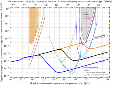
Figure 2: Final GW spectrum for three parameter examples (see Fig. 3) alongside the power-law integrated sensitivity curves Thrane:2013oya of existing and upcoming GW experiments.

Discussion. Our results in Fig. 3 are a powerful testament to the complementarity of future GW experiments. Consider, e.g., a scalar field with $m_{\phi}=10\,\textrm{GeV}$, $\Gamma_{\phi}=10\,\textrm{eV}$, and $\phi_{\rm ini}=10^{18}\,\textrm{GeV}$ (point ➁ in Fig. 3). In this case, the scalar era occurs at temperatures $5.4\times 10^{4}\lesssim T/\textrm{GeV}\lesssim 1.7\times 10^{8}$, which leads to a dilution factor $D\simeq 7.9\times 10^{-2}$ and a modification of the GW spectrum at frequencies $1.6\times 10^{-3}\lesssim f/\textrm{Hz}\lesssim 4.9\times 10^{-1}$. This scenario can be directly probed by LISA, DECIGO, and BBO, all of which will observe a departure from a pure power law. At the same time, CE, IPTA, and SKA will detect the SGWB from inflation, while HLVK and ET will fail to observe a primordial signal. On top of that, future CMB observations may confirm the blue tilt of the tensor spectrum. Along these lines, it is possible to translate every point in Fig. 3 into a list of predictions, i.e., a characteristic experimental fingerprint, for the GW experiments that we have considered in this paper.

The results of our analysis are applicable to a wide range of particle physics models that lead to a scalar era in the early Universe. In addition, it is important to note that the modified expansion history and late-time entropy production during the scalar era not only affect the spectrum of primordial GWs, but also the evolution of other cosmological relics, such as dark matter Hashimoto:1998ua ; Giudice:2000ex ; Acharya:2009zt ; Monteux:2015qqa ; Co:2015pka ; Roszkowski:2015psa ; Hamdan:2017psw ; Nelson:2018via and the baryon asymmetry of the Universe Chen:2019wnk . Finding evidence for a scalar era in future GW experiments would therefore have a profound impact on our understanding of BSM physics and early-Universe cosmology alike.

The analysis presented in this paper should only be regarded as a first step. Next, it will be necessary to relax our assumptions regarding the primordial tensor spectrum, the initial field value, and the shape of the scalar potential. Aside from that, it would be interesting to identify a self-consistent embedding of our scenario in a concrete inflationary model that is capable of generating a strongly blue-tilted tensor spectrum. We leave these steps for future work, concluding with the observation that a scalar era in the early Universe represents a fascinating possibility that awaits further exploration.

Acknowledgements. We thank Sachiko Kuroyanagi for sharing with us her numerical results on the DECIGO overlap reduction function; Ken’ichi Saikawa and Satoshi Shirai for sharing with us their numerical results on the GW transfer function at frequencies below $1\,\textrm{nHz}$, which takes into account damping effects caused by free-streaming photons and neutrinos at low temperatures; and Hirotaka Yuzurihara for useful comments on the KAGRA sensitivity curve. We are grateful to all of these authors as well as to Kohei Kamada, Marco Peloso, and Angelo Ricciardone for helpful discussions. This project has received funding/support from the European Union’s Horizon 2020 research and innovation programme under the Marie Skłodowska-Curie grant agreement No. 690575. This work was supported by INFN through the “Theoretical Astroparticle Physics” (TAsP) project.

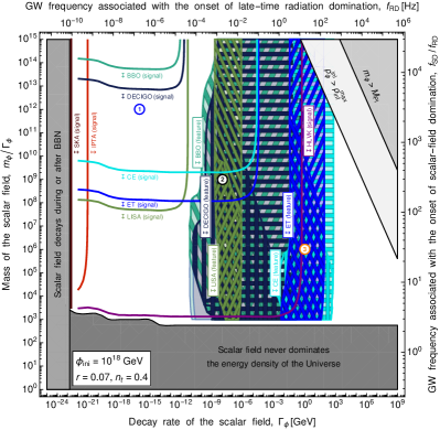
Figure 3: Experimental prospects to observe a signal or a even a feature in the GW spectrum (see text for details) in dependence of the model parameters $m_{\phi}$ and $\Gamma_{\phi}$. The three points ➀, ➁, ➂ mark the parameter examples used in Figs. 1 and 2. The meshes drawn in the feature regions indicate where the frequencies $f_{\rm RD}$ (meshes extending up to arbitrarily large $m_{\phi}$) and $f_{\rm SD}$ (meshes extending up to a finite $m_{\phi}$) fall into the frequency ranges of the individual experiments (see Fig. 2).

References

- (1) LIGO Scientific, Virgo Collaboration, B. P. Abbott et al., Observation of Gravitational Waves from a Binary Black Hole Merger, Phys. Rev. Lett. 116 (2016), no. 6 061102, [arXiv:1602.03837].
- (2) LIGO Scientific Collaboration, G. M. Harry, Advanced LIGO: The next generation of gravitational wave detectors, Class. Quant. Grav. 27 (2010) 084006.
- (3) LIGO Scientific Collaboration, J. Aasi et al., Advanced LIGO, Class. Quant. Grav. 32 (2015) 074001, [arXiv:1411.4547].
- (4) VIRGO Collaboration, F. Acernese et al., Advanced Virgo: a second-generation interferometric gravitational wave detector, Class. Quant. Grav. 32 (2015), no. 2 024001, [arXiv:1408.3978].
- (5) LIGO Scientific, Virgo Collaboration, B. P. Abbott et al., GWTC-1: A Gravitational-Wave Transient Catalog of Compact Binary Mergers Observed by LIGO and Virgo during the First and Second Observing Runs, arXiv:1811.12907.
- (6) M. Maggiore, Gravitational wave experiments and early universe cosmology, Phys. Rept. 331 (2000) 283–367, [gr-qc/9909001].
- (7) S. T. McWilliams, R. Caldwell, K. Holley-Bockelmann, S. L. Larson, and M. Vallisneri, Astro2020 Decadal Science White Paper: The state of gravitational-wave astrophysics in 2020, arXiv:1903.04592.
- (8) R. Caldwell et al., Astro2020 Science White Paper: Cosmology with a Space-Based Gravitational Wave Observatory, arXiv:1903.04657.
- (9) V. Kalogera et al., Deeper, Wider, Sharper: Next-Generation Ground-Based Gravitational-Wave Observations of Binary Black Holes, arXiv:1903.09220.
- (10) N. J. Cornish, E. Berti, K. Holley-Bockelmann, S. Larson, S. McWilliams, G. Mueller, P. Natarajan, and M. Vallisneri, The Discovery Potential of Space-Based Gravitational Wave Astronomy, arXiv:1904.01438.
- (11) LIGO Scientific Collaboration, D. Shoemaker et al., Gravitational wave astronomy with LIGO and similar detectors in the next decade, arXiv:1904.03187.
- (12) C. Caprini and D. G. Figueroa, Cosmological Backgrounds of Gravitational Waves, Class. Quant. Grav. 35 (2018), no. 16 163001, [arXiv:1801.04268].
- (13) N. Christensen, Stochastic Gravitational Wave Backgrounds, Rept. Prog. Phys. 82 (2019), no. 1 016903, [arXiv:1811.08797].
- (14) M. Geller, A. Hook, R. Sundrum, and Y. Tsai, Primordial Anisotropies in the Gravitational Wave Background from Cosmological Phase Transitions, Phys. Rev. Lett. 121 (2018), no. 20 201303, [arXiv:1803.10780].
- (15) L. P. Grishchuk, Amplification of gravitational waves in an istropic universe, Sov. Phys. JETP 40 (1975) 409–415.
- (16) A. A. Starobinsky, Spectrum of relict gravitational radiation and the early state of the universe, JETP Lett. 30 (1979) 682–685.
- (17) V. A. Rubakov, M. V. Sazhin, and A. V. Veryaskin, Graviton Creation in the Inflationary Universe and the Grand Unification Scale, Phys. Lett. 115B (1982) 189–192.
- (18) M. C. Guzzetti, N. Bartolo, M. Liguori, and S. Matarrese, Gravitational waves from inflation, Riv. Nuovo Cim. 39 (2016), no. 9 399–495, [arXiv:1605.01615].
- (19) N. Seto and J. Yokoyama, Probing the equation of state of the early universe with a space laser interferometer, J. Phys. Soc. Jap. 72 (2003) 3082–3086, [gr-qc/0305096].
- (20) L. A. Boyle and P. J. Steinhardt, Probing the early universe with inflationary gravitational waves, Phys. Rev. D77 (2008) 063504, [astro-ph/0512014].
- (21) L. A. Boyle and A. Buonanno, Relating gravitational wave constraints from primordial nucleosynthesis, pulsar timing, laser interferometers, and the CMB: Implications for the early Universe, Phys. Rev. D78 (2008) 043531, [arXiv:0708.2279].
- (22) S. Kuroyanagi, T. Chiba, and N. Sugiyama, Precision calculations of the gravitational wave background spectrum from inflation, Phys. Rev. D79 (2009) 103501, [arXiv:0804.3249].
- (23) K. Nakayama and J. Yokoyama, Gravitational Wave Background and Non-Gaussianity as a Probe of the Curvaton Scenario, JCAP 1001 (2010) 010, [arXiv:0910.0715].
- (24) S. Kuroyanagi, C. Ringeval, and T. Takahashi, Early universe tomography with CMB and gravitational waves, Phys. Rev. D87 (2013), no. 8 083502, [arXiv:1301.1778].
- (25) R. Jinno, T. Moroi, and K. Nakayama, Inflationary Gravitational Waves and the Evolution of the Early Universe, JCAP 1401 (2014) 040, [arXiv:1307.3010].
- (26) K. Saikawa and S. Shirai, Primordial gravitational waves, precisely: The role of thermodynamics in the Standard Model, JCAP 1805 (2018), no. 05 035, [arXiv:1803.01038].
- (27) K. Nakayama, S. Saito, Y. Suwa, and J. Yokoyama, Space laser interferometers can determine the thermal history of the early Universe, Phys. Rev. D77 (2008) 124001, [arXiv:0802.2452].
- (28) K. Nakayama, S. Saito, Y. Suwa, and J. Yokoyama, Probing reheating temperature of the universe with gravitational wave background, JCAP 0806 (2008) 020, [arXiv:0804.1827].
- (29) S. Kuroyanagi, K. Nakayama, and S. Saito, Prospects for determination of thermal history after inflation with future gravitational wave detectors, Phys. Rev. D84 (2011) 123513, [arXiv:1110.4169].
- (30) W. Buchmüller, V. Domcke, K. Kamada, and K. Schmitz, The Gravitational Wave Spectrum from Cosmological Breaking, JCAP 1310 (2013) 003, [arXiv:1305.3392].
- (31) W. Buchmuller, V. Domcke, K. Kamada, and K. Schmitz, A Minimal Supersymmetric Model of Particle Physics and the Early Universe, arXiv:1309.7788.
- (32) R. Jinno, T. Moroi, and T. Takahashi, Studying Inflation with Future Space-Based Gravitational Wave Detectors, JCAP 1412 (2014), no. 12 006, [arXiv:1406.1666].
- (33) S. Kuroyanagi, K. Nakayama, and J. Yokoyama, Prospects of determination of reheating temperature after inflation by DECIGO, PTEP 2015 (2015), no. 1 013E02, [arXiv:1410.6618].
- (34) S. Schettler, T. Boeckel, and J. Schaffner-Bielich, Imprints of the QCD Phase Transition on the Spectrum of Gravitational Waves, Phys. Rev. D83 (2011) 064030, [arXiv:1010.4857].
- (35) F. Hajkarim, J. Schaffner-Bielich, S. Wystub, and M. M. Wygas, Effects of the QCD Equation of State and Lepton Asymmetry on Primordial Gravitational Waves, Phys. Rev. D99 (2019), no. 10 103527, [arXiv:1904.01046].
- (36) R. Jinno, T. Moroi, and K. Nakayama, Probing dark radiation with inflationary gravitational waves, Phys. Rev. D86 (2012) 123502, [arXiv:1208.0184].
- (37) R. R. Caldwell, T. L. Smith, and D. G. E. Walker, Using a Primordial Gravitational Wave Background to Illuminate New Physics, arXiv:1812.07577.
- (38) Y. Cui, M. Lewicki, D. E. Morrissey, and J. D. Wells, Cosmic Archaeology with Gravitational Waves from Cosmic Strings, Phys. Rev. D97 (2018), no. 12 123505, [arXiv:1711.03104].
- (39) Y. Cui, M. Lewicki, D. E. Morrissey, and J. D. Wells, Probing the pre-BBN universe with gravitational waves from cosmic strings, JHEP 01 (2019) 081, [arXiv:1808.08968].
- (40) Y. Matsui and S. Kuroyanagi, Gravitational wave background from kink-kink collisions on infinite cosmic strings, arXiv:1902.09120.
- (41) G. D. Coughlan, W. Fischler, E. W. Kolb, S. Raby, and G. G. Ross, Cosmological Problems for the Polonyi Potential, Phys. Lett. 131B (1983) 59–64.
- (42) J. R. Ellis, D. V. Nanopoulos, and M. Quiros, On the Axion, Dilaton, Polonyi, Gravitino and Shadow Matter Problems in Supergravity and Superstring Models, Phys. Lett. B174 (1986) 176–182.
- (43) B. de Carlos, J. A. Casas, F. Quevedo, and E. Roulet, Model independent properties and cosmological implications of the dilaton and moduli sectors of 4-d strings, Phys. Lett. B318 (1993) 447–456, [hep-ph/9308325].
- (44) T. Moroi and L. Randall, Wino cold dark matter from anomaly mediated SUSY breaking, Nucl. Phys. B570 (2000) 455–472, [hep-ph/9906527].
- (45) R. Durrer and J. Hasenkamp, Testing Superstring Theories with Gravitational Waves, Phys. Rev. D84 (2011) 064027, [arXiv:1105.5283].
- (46) G. Kane, K. Sinha, and S. Watson, Cosmological Moduli and the Post-Inflationary Universe: A Critical Review, Int. J. Mod. Phys. D24 (2015), no. 08 1530022, [arXiv:1502.07746].
- (47) C. D. Froggatt and H. B. Nielsen, Hierarchy of Quark Masses, Cabibbo Angles and CP Violation, Nucl. Phys. B147 (1979) 277–298.
- (48) T. Kugo, I. Ojima, and T. Yanagida, Superpotential Symmetries and Pseudo-Nambu-Goldstone Supermultiplets, Phys. Lett. 135B (1984) 402–408.
- (49) T. Banks, M. Dine, and M. Graesser, Supersymmetry, axions and cosmology, Phys. Rev. D68 (2003) 075011, [hep-ph/0210256].
- (50) M. Kawasaki and K. Nakayama, Solving Cosmological Problems of Supersymmetric Axion Models in Inflationary Universe, Phys. Rev. D77 (2008) 123524, [arXiv:0802.2487].
- (51) K. Harigaya, M. Ibe, K. Schmitz, and T. T. Yanagida, Peccei-Quinn symmetry from a gauged discrete R symmetry, Phys. Rev. D88 (2013), no. 7 075022, [arXiv:1308.1227].
- (52) K. Harigaya, M. Ibe, K. Schmitz, and T. T. Yanagida, Peccei-Quinn Symmetry from Dynamical Supersymmetry Breaking, Phys. Rev. D92 (2015), no. 7 075003, [arXiv:1505.07388].
- (53) R. T. Co, F. D’Eramo, and L. J. Hall, Supersymmetric axion grand unified theories and their predictions, Phys. Rev. D94 (2016), no. 7 075001, [arXiv:1603.04439].
- (54) R. T. Co, F. D’Eramo, L. J. Hall, and K. Harigaya, Saxion Cosmology for Thermalized Gravitino Dark Matter, JHEP 07 (2017) 125, [arXiv:1703.09796].
- (55) Planck Collaboration, Y. Akrami et al., Planck 2018 results. X. Constraints on inflation, arXiv:1807.06211.
- (56) J. L. Cook and L. Sorbo, Particle production during inflation and gravitational waves detectable by ground-based interferometers, Phys. Rev. D85 (2012) 023534, [arXiv:1109.0022]. [Erratum: Phys. Rev.D86,069901(2012)].
- (57) N. Barnaby, E. Pajer, and M. Peloso, Gauge Field Production in Axion Inflation: Consequences for Monodromy, non-Gaussianity in the CMB, and Gravitational Waves at Interferometers, Phys. Rev. D85 (2012) 023525, [arXiv:1110.3327].
- (58) M. M. Anber and L. Sorbo, Non-Gaussianities and chiral gravitational waves in natural steep inflation, Phys. Rev. D85 (2012) 123537, [arXiv:1203.5849].
- (59) V. Domcke, M. Pieroni, and P. Binétruy, Primordial gravitational waves for universality classes of pseudoscalar inflation, JCAP 1606 (2016) 031, [arXiv:1603.01287].
- (60) D. Jiménez, K. Kamada, K. Schmitz, and X.-J. Xu, Baryon asymmetry and gravitational waves from pseudoscalar inflation, JCAP 1712 (2017), no. 12 011, [arXiv:1707.07943].
- (61) A. Papageorgiou, M. Peloso, and C. Unal, Nonlinear perturbations from axion-gauge fields dynamics during inflation, JCAP 1907 (2019), no. 07 004, [arXiv:1904.01488].
- (62) LIGO Scientific, Virgo Collaboration, B. P. Abbott et al., Upper Limits on the Stochastic Gravitational-Wave Background from Advanced LIGO’s First Observing Run, Phys. Rev. Lett. 118 (2017), no. 12 121101, [arXiv:1612.02029]. [Erratum: Phys. Rev. Lett.119,no.2,029901(2017)].
- (63) LIGO Scientific, Virgo Collaboration, A search for the isotropic stochastic background using data from Advanced LIGO’s second observing run, arXiv:1903.02886.
- (64) S. Kuroyanagi, T. Takahashi, and S. Yokoyama, Blue-tilted Tensor Spectrum and Thermal History of the Universe, JCAP 1502 (2015) 003, [arXiv:1407.4785].
- (65) P. D. Lasky et al., Gravitational-wave cosmology across 29 decades in frequency, Phys. Rev. X6 (2016), no. 1 011035, [arXiv:1511.05994].
- (66) D. J. Fixsen, The Temperature of the Cosmic Microwave Background, Astrophys. J. 707 (2009) 916–920, [arXiv:0911.1955].
- (67) T. S. Bunch and P. C. W. Davies, Quantum Field Theory in de Sitter Space: Renormalization by Point Splitting, Proc. Roy. Soc. Lond. A360 (1978) 117–134.
- (68) A. D. Linde, Scalar Field Fluctuations in Expanding Universe and the New Inflationary Universe Scenario, Phys. Lett. 116B (1982) 335–339.
- (69) I. Affleck and M. Dine, A New Mechanism for Baryogenesis, Nucl. Phys. B249 (1985) 361–380.
- (70) A. A. Starobinsky and J. Yokoyama, Equilibrium state of a selfinteracting scalar field in the De Sitter background, Phys. Rev. D50 (1994) 6357–6368, [astro-ph/9407016].
- (71) M. S. Turner, M. J. White, and J. E. Lidsey, Tensor perturbations in inflationary models as a probe of cosmology, Phys. Rev. D48 (1993) 4613–4622, [astro-ph/9306029].
- (72) Y. Watanabe and E. Komatsu, Improved Calculation of the Primordial Gravitational Wave Spectrum in the Standard Model, Phys. Rev. D73 (2006) 123515, [astro-ph/0604176].
- (73) B. Allen and J. D. Romano, Detecting a stochastic background of gravitational radiation: Signal processing strategies and sensitivities, Phys. Rev. D59 (1999) 102001, [gr-qc/9710117].
- (74) KAGRA Collaboration, K. Somiya, Detector configuration of KAGRA: The Japanese cryogenic gravitational-wave detector, Class. Quant. Grav. 29 (2012) 124007, [arXiv:1111.7185].
- (75) KAGRA Collaboration, Y. Aso, Y. Michimura, K. Somiya, M. Ando, O. Miyakawa, T. Sekiguchi, D. Tatsumi, and H. Yamamoto, Interferometer design of the KAGRA gravitational wave detector, Phys. Rev. D88 (2013), no. 4 043007, [arXiv:1306.6747].
- (76) LIGO Scientific Collaboration, B. P. Abbott et al., Exploring the Sensitivity of Next Generation Gravitational Wave Detectors, Class. Quant. Grav. 34 (2017), no. 4 044001, [arXiv:1607.08697].
- (77) M. Punturo et al., The Einstein Telescope: A third-generation gravitational wave observatory, Class. Quant. Grav. 27 (2010) 194002.
- (78) S. Hild et al., Sensitivity Studies for Third-Generation Gravitational Wave Observatories, Class. Quant. Grav. 28 (2011) 094013, [arXiv:1012.0908].
- (79) B. Sathyaprakash et al., Scientific Objectives of Einstein Telescope, Class. Quant. Grav. 29 (2012) 124013, [arXiv:1206.0331]. [Erratum: Class. Quant. Grav.30,079501(2013)].
- (80) LISA Collaboration, H. Audley et al., Laser Interferometer Space Antenna, arXiv:1702.00786.
- (81) N. Seto, S. Kawamura, and T. Nakamura, Possibility of direct measurement of the acceleration of the universe using 0.1-Hz band laser interferometer gravitational wave antenna in space, Phys. Rev. Lett. 87 (2001) 221103, [astro-ph/0108011].
- (82) S. Kawamura et al., The Japanese space gravitational wave antenna DECIGO, Class. Quant. Grav. 23 (2006) S125–S132.
- (83) J. Crowder and N. J. Cornish, Beyond LISA: Exploring future gravitational wave missions, Phys. Rev. D72 (2005) 083005, [gr-qc/0506015].
- (84) V. Corbin and N. J. Cornish, Detecting the cosmic gravitational wave background with the big bang observer, Class. Quant. Grav. 23 (2006) 2435–2446, [gr-qc/0512039].
- (85) G. M. Harry, P. Fritschel, D. A. Shaddock, W. Folkner, and E. S. Phinney, Laser interferometry for the big bang observer, Class. Quant. Grav. 23 (2006) 4887–4894. [Erratum: Ibid. 23 (2006) 7361].
- (86) G. Hobbs et al., The international pulsar timing array project: using pulsars as a gravitational wave detector, Class. Quant. Grav. 27 (2010) 084013, [arXiv:0911.5206].
- (87) R. N. Manchester, The International Pulsar Timing Array, Class. Quant. Grav. 30 (2013) 224010, [arXiv:1309.7392].
- (88) J. P. W. Verbiest et al., The International Pulsar Timing Array: First Data Release, Mon. Not. Roy. Astron. Soc. 458 (2016), no. 2 1267–1288, [arXiv:1602.03640].
- (89) C. L. Carilli and S. Rawlings, Science with the Square Kilometer Array: Motivation, key science projects, standards and assumptions, New Astron. Rev. 48 (2004) 979, [astro-ph/0409274].
- (90) G. Janssen et al., Gravitational wave astronomy with the SKA, PoS AASKA14 (2015) 037, [arXiv:1501.00127].
- (91) P. Bull et al., Fundamental Physics with the Square Kilometer Array, arXiv:1810.02680.
- (92) X. Siemens, J. Ellis, F. Jenet, and J. D. Romano, The stochastic background: scaling laws and time to detection for pulsar timing arrays, Class. Quant. Grav. 30 (2013) 224015, [arXiv:1305.3196].
- (93) T. Robson, N. J. Cornish, and C. Liug, The construction and use of LISA sensitivity curves, Class. Quant. Grav. 36 (2019), no. 10 105011, [arXiv:1803.01944].
- (94) S. Kuroyanagi, T. Chiba, and T. Takahashi, Probing the Universe through the Stochastic Gravitational Wave Background, JCAP 1811 (2018), no. 11 038, [arXiv:1807.00786].
- (95) E. Thrane and J. D. Romano, Sensitivity curves for searches for gravitational-wave backgrounds, Phys. Rev. D88 (2013), no. 12 124032, [arXiv:1310.5300].
- (96) M. Hashimoto, K. I. Izawa, M. Yamaguchi, and T. Yanagida, Axion cosmology with its scalar superpartner, Phys. Lett. B437 (1998) 44–50, [hep-ph/9803263].
- (97) G. F. Giudice, E. W. Kolb, and A. Riotto, Largest temperature of the radiation era and its cosmological implications, Phys. Rev. D64 (2001) 023508, [hep-ph/0005123].
- (98) B. S. Acharya, G. Kane, S. Watson, and P. Kumar, A Non-thermal WIMP Miracle, Phys. Rev. D80 (2009) 083529, [arXiv:0908.2430].
- (99) A. Monteux and C. S. Shin, Thermal Goldstino Production with Low Reheating Temperatures, Phys. Rev. D92 (2015) 035002, [arXiv:1505.03149].
- (100) R. T. Co, F. D’Eramo, L. J. Hall, and D. Pappadopulo, Freeze-In Dark Matter with Displaced Signatures at Colliders, JCAP 1512 (2015), no. 12 024, [arXiv:1506.07532].
- (101) L. Roszkowski, S. Trojanowski, and K. Turzynski, Axino dark matter with low reheating temperature, JHEP 11 (2015) 139, [arXiv:1507.06164].
- (102) S. Hamdan and J. Unwin, Dark Matter Freeze-out During Matter Domination, Mod. Phys. Lett. A33 (2018), no. 29 1850181, [arXiv:1710.03758].
- (103) A. E. Nelson and H. Xiao, Axion Cosmology with Early Matter Domination, Phys. Rev. D98 (2018), no. 6 063516, [arXiv:1807.07176].
- (104) M.-C. Chen, S. Ipek, and M. Ratz, Baryogenesis From Flavon Decays, arXiv:1903.06211.