Efficient Distributed Community Detection in the Stochastic Block Model

Abstract

Designing effective algorithms for community detection is an important and challenging problem in large-scale graphs, studied extensively in the literature. Various solutions have been proposed, but many of them are centralized with expensive procedures (requiring full knowledge of the input graph) and have a large running time.

In this paper, we present a distributed algorithm for community detection in the stochastic block model (also called planted partition model), a widely-studied and canonical random graph model for community detection and clustering. Our algorithm called CDRW(Community Detection by Random Walks) is based on random walks, and is localized and lightweight, and easy to implement. A novel feature of the algorithm is that it uses the concept of local mixing time to identify the community around a given node.

We present a rigorous theoretical analysis that shows that the algorithm can accurately identify the communities in the stochastic block model and characterize the model parameters where the algorithm works. We also present experimental results that validate our theoretical analysis. We also analyze the performance of our distributed algorithm under the CONGEST distributed model as well as the $k$-machine model, a model for large-scale distributed computations, and show that it can be efficiently implemented.

I introduction

Finding communities in networks (graphs) is an important problem and has been extensively studied in the last two decades, e.g., see the surveys [1, 10, 17, 18] and other references in Section II. At a high level, the goal is to identify subsets of vertices of the given graph so that each subset represents a “community.” While there are differences in how communities are defined exactly (e.g., subsets defining a community may overlap or not), a uniform property that underlies most definitions is that there are more edges connecting nodes within a subset than edges connecting to outside the subset. Thus, this captures the fact that a community is somehow more “well-connected” with respect to itself compared to the rest of the graph. One way to express this property formally is by using the notion of conductance (defined in Section I-C) which (informally) measures the ratio of the total degree going out of the subset to the total degree among all nodes in the subset. A community subset will have generally low conductance (also sometime referred to as a “sparse” cut). Another way to measure this is by using the notion of modularity [35] which (informally) measures how well connected a subset is compared to the random graph that can be embedded within the set. A vertex subset that has a high modularity value can be considered a community according to this measure.

Designing effective algorithms for community detection in graphs is an important and challenging problem. With the rise of massive graphs such as the Web graph, social networks, biological networks, finding communities (or clusters) in large-scale graphs efficiently is becoming even more important [10, 15, 18, 20, 35]. In particular, understanding the community structure is a key issue in many applications in various complex networks including biological and social networks (see e.g., [10] and the references therein).

Various solutions have been proposed (cf. Section II), but many of them are centralized with expensive procedures (requiring full knowledge of the input graph) and have a large running time [10]. In particular, the problem of detecting (identifying) communities in the stochastic block model (SBM) [1, 10] has been extensively studied in the literature (cf. Section II). The stochastic block model (defined formally in Section I-B), also known as the planted partition model (PPM) is a widely-used random graph model in community detection and clustering studies (see e.g., [1, 8, 25]). Informally, in the PPM model, we are given a graph $G$ on $n$ nodes which are partitioned into a set of $r$ communities (each is a random graph on $n/r$ vertices) and these communities are interconnected by random edges. The total number of edges within a community (intra-community edges) is typically much more than the number of edges between communities (inter-community edges). The main goal is to devise algorithms to identify the $r$ communities that are “planted” in the graph. Several algorithms have been devised for this model, but as mentioned earlier, they are mostly centralized (with some exceptions — cf. Section II) with large running time. There are few distributed algorithms (see e.g., [10, 27]) but either they are shown to work only when the number of communities is small (typically 2) [10]) or when the communities are very dense[27]). In particular, to the best of our knowledge, (prior to this work) there is no rigorous analysis of community detection algorithms in distributed large-scale graph processing models such as MapReduce and Massively Parallel Computing (MPC) model [24], and the $k$-machine model [26].

I-A Our Contributions

In this paper, we present a novel distributed algorithm, called CDRW (Community Detection via Random Walks) for detecting communities in the PPM model[12]. Our algorithm is based on the recently proposed local mixing paradigm [33] (see Section I-C for a formal definition) to detect community structure in sparse (bounded-degree) graphs. Informally, a local mixing set is one where a random walk started at some node in the set mixes well with respect to this set. The intuition in using this concept for community detection is that since a community is well-connected, it has good expansion within the community and hence a random walk started at a node in the community mixes well within the community. The notion of “mixes well” is captured by the fact that the random walk reaches close to the stationary distribution when restricted to the nodes in the community subset [33]. Since the main tool for this algorithm uses random walks which is local and lightweight, it is easy to implement this algorithm in a distributed manner. We will analyze the performance of the algorithm in two distributed computing models, namely the standard CONGEST model of distributed computing [40] and the $k$-machine model [26], which is a model for large-scale distributed computations. We show that CDRW can be implemented efficiently in both models (cf. Theorem 6 and Section III-B). The $k$-machine model implementation is especially suitable for large-scale graphs and thus can be used in community detection in large SBM graphs. In particular, we show that the round complexity in the $k$-machine model (cf. Section III-B) scales quadractically (i.e., $k^{-2}$) in the number of machines when the graph is sparse and linearly (i.e.,$k^{-1}$) in general.

As is usual in community detection, a main focus is analyzing the effectiveness of the algorithm in finding communities. We present a rigorous theoretical analysis that shows that CDRW algorithm can accurately identify the communities in the PPM, which is a popular and widely-studied random graph model for community detection analysis [1]. A PPM model (cf. Section I-B) is a parameterized random graph model which has a built-in community structure. Each community has high expansion within the community and forms a low conductance subset (and hence relatively less edges go outside the community); the expansion, conductance, and edge density can be controlled by varying the parameters. CDRW does well when the number of intra-community edges is much more than the number of inter-community edges (these are controlled by the parameters of the model). Our theoretical analysis (cf. Theorem 6 for the precise statement) quantitatively characterizes when CDRW does well vis-a-vis the parameters of the model. Our results improve over previous distributed algorithms that have been proposed for the PPM model ([10]) both in the number of communities that can be provably detected as well as range of parameters where accurate detection is possible; they also improve on previous results that provably work only on dense PPM graphs [27] (details in Section II).

We also present extensive simulations of our algorithm in the PPM model under various parameters. Experimental results on the model validate our theoretical analysis; in fact experiments show that CDRW works relatively well in identifying communities even under less stringent parameters.

I-B Model, Definitions, and Preliminaries

I-B1 Graph Model

We describe the stochastic block model (SBM) [21], a well-studied random graph model that is used in community detection analysis. Before that we recall the Erdős-Rényi random graph model [16], a basic random graph model, that the SBM model builds on. In the Erdős-Rényi random graph model, also known as the $G_{np}$ model, each of $\binom{n}{2}$ possible edges is present in the graph independently with probability $p$. The $G_{np}$ random graph has close to uniform degree (the expected degree of a node is $(n-1)p$) and a well-known fact about $G(n,p)$ is that if $p=\Theta(\log n/n)$ the graph is connected with high probability and its degree is concentrated at its expectation. In the SBM model, the vertices are partitioned into $r$ disjoint community sets ($r$ is a parameter). Let $c(u)$ denote the community that node $u$ belongs to. If two nodes $u$ and $v$ belong to the same community (i.e., $c(u)=c(v)$), they connect independently with probability $p_{c(u)}$ (independent of other nodes). If they belong to different communities, they connect independently with probability $p_{c(u),c(v)}$. A SBM model has a separable community structure [1] if it has a higher value of intra- than inter-community connectivity probability. A commonly used version of SBM model that is called Planted Partition Model (PPM), denoted as $G_{npq}$ [11, 21] is usually used as a benchmark. A symmetric $G_{npq}$ with $r$ blocks is composed of $r$ exclusive set of nodes in $\mathcal{C}=<C_{1},C_{2},\dots,C_{r}>$, where $\cup_{i=1}^{i=r}C_{i}=V,\ |C_{i}|=|C_{j}|\text{ and }C_{i}\cap C_{j}=\emptyset\text{ when }i\neq j$. In $G_{npq}$, each possible edge $e(u,v)$ is independently present with probability $p$ if both ends of $u$ and $v$ belong to the same block $C_{i}$, otherwise with probability $q$. Figure 1 shows a PPM of $5$ blocks ($r=5$), each containing $200$ nodes. For the PPM model, each of the $r$ communities induce a $n/r$-vertex subgraph which is a $G(n/r,p)$ random graph. The goal of community detection in the PPM (or SBM) model is to identify the $r$ community sets. This problem has been widely studied [1].

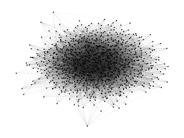
(a) A PPM graph shown without its ground-truth communities.

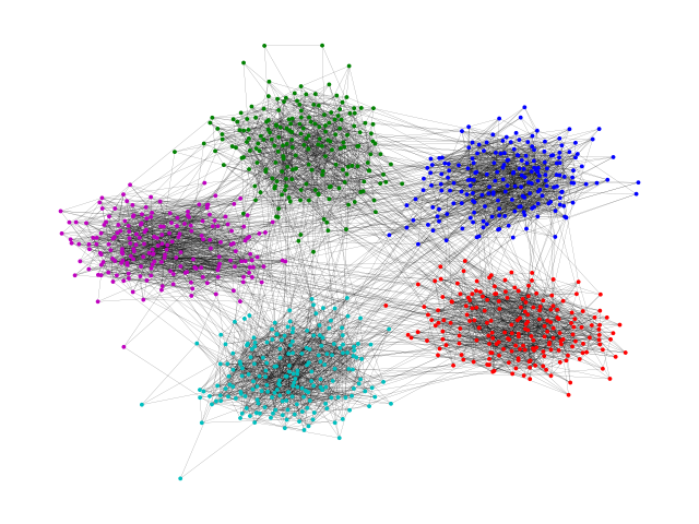
(b) Redrawing of the same PPM graph showing the communities.

Figure 1: Both of the above graphs are the same PPM graph. The graph size is $n=1000$, number of communities $r=5$, the existence probability of intra(inter) community edges is $p=\frac{1}{20}$($q=\frac{1}{1000})$ as in [1, Figure 1]. We highlight ground truth communities in different colors in Figure1(b).

I-B2 Distributed Computing Models

We consider two distributed computing models and analyze the complexity of the algorithm’s implementation under both the models.

CONGEST model. This is a standard and widely-studied CONGEST model of distributed computing [37, 40], which captures the bandwidth constraints inherent in real-world networks. The distributed network is modelled as an undirected and unweighted graph $G=(V,E)$, where $|V|=n$ and $|E|=m$, where nodes represent processors (or computing entities) and the edges represent communication links. In this paper, $G$ will be a graph belonging to the PPM model. Each node is associated with a distinct label or ID (e.g., its IP address). Nodes communicate through the edges in synchronous rounds; in every round, each node is allowed to send a message of size at most $O(\log n)$ bits to each of its neighbors. The message will arrive to the receiver nodes at the end of the current round. Initially every node has limited knowledge; it only knows its own ID and its neighbors IDs. In addition, it may known additional parameters of the graph such as $n,m,D$ (where $D$ is the diameter). The two standard complexity of an algorithm are the time and message complexity in the CONGEST model. While time complexity measures the number of rounds taken by the algorithm, the message complexity measures the total number of messages exchanged during the course of the algorithm.

$k$-machine model. The $k$-machine model (a.k.a. Big Data model) is a model for large-scale distributed computing introduced in [26] and studied in various papers [3, 23, 26, 38, 39]. In this model, the input graph (or more generally, any other type of data) is distributed across a group of $k\geq 2$ machines that are pairwise interconnected via a communication network. The $k$ machines jointly perform computations on an arbitrary $n$-vertex, $m$-edge input graph (where typically $n,m\gg k$) distributed among the machines (randomly or in a balanced fashion). The communication is point-to-point via message passing. Machines do not share any memory and have no other means of communication. The computation advances in synchronous rounds, and each link is assumed to have a bandwidth of $B$ bits per round, i.e., $B$ bits can be transmitted over each link in each round; unless otherwise stated, we assume $B=O(\log n)$ (where $n$ is the input size) [38, 39]. The goal is to minimize the round complexity, i.e., the number of communication rounds required by the computation.

Initially, the entire graph $G$ is not known by any single machine, but rather partitioned among the $k$ machines in a “balanced” fashion, i.e., the nodes and/or edges of $G$ are partitioned approximately evenly among the machines. We assume a vertex-partition model, whereby vertices, along with information of their incident edges, are partitioned across machines. Specifically, the type of partition that we will assume throughout is the random vertex partition (RVP), that is, each vertex of the input graph is assigned randomly to one machine. (This is the typical way used by many real systems, such as Pregel [31], to initially distribute the input graph among the machines.) If a vertex $v$ is assigned to machine $M_{i}$ we say that $M_{i}$ is the home machine of $v$. A convenient way to implement the RVP model is through hashing: each vertex (ID) is hashed to one of the $k$ machines. Hence, if a machine knows a vertex ID, it also knows where it is hashed to. It can be shown that the RVP model results in (essentially) a balanced partition of the graph: each machine gets $\tilde{O}(n/k)$ vertices and $\tilde{O}(m/k+\Delta)$ edges, where $\Delta$ is the maximum degree.

At the end of the computation, for the community detection problem, the community that each vertex belongs to will be output by some machine.

I-C Random Walk Preliminaries and Local Mixing Set

Our algorithm is based on the mixing property of a random walk in a graph. We use the notion of local mixing set of a random walk, introduced in [33], to identify communities in a graph. Let us define random walk preliminaries, local mixing time, and local mixing set as defined in [33]. Given an undirected graph and a source node $s$, a simple random walk is defined as: in each step, the walk goes from the current node to a random neighbor i.e., from the current node $u$, the probability of moving to node $v$ is $\Pr(u,v)=1/d(u)$ if $(u,v)\in E$, otherwise $\Pr(u,v)=0$, where $d(u)$ is the degree of $u$. Let $\mathbf{p}_{t}(s)$ be the probability distribution at time $t$ starting from the source node $s$. Then $\mathbf{p}_{0}(s)$ is the initial distribution with probability $1$ at the node $s$ and zero at all other nodes. The $\mathbf{p}_{t}(s)$ can be seen as the matrix-vector multiplication between $(A)^{t}$ and $\mathbf{p}_{0}(s)$, where $A$ is the transpose of the transition matrix of $G$. Let $p_{t}(s,v)$ be the probability that the random walk be in node $v$ after $t$ steps. When it’s clear from the context we omit the source node from the notations and denote it by $p_{t}(v)$ only. The stationary distribution (a.k.a steady-state distribution) is the probability distribution which doesn’t change anymore (i.e., it has converged). The stationary distribution of an undirected connected graph is a well-defined quantity which is $\bigl{(}\frac{d(v_{1})}{2m},\frac{d(v_{2})}{2m},\ldots,\frac{d(v_{n})}{2m}\bigr{)}$, where $d(v_{i})$ is the degree of node $v_{i}$. We denote the stationary distribution vector by $\boldsymbol{\pi}$, i.e., $\pi(v)=d(v)/2m$ for each node $v$. The stationary distribution of a graph is fixed irrespective of the starting node of a random walk, however, the number of steps (i.e., time) to reach to the stationary distribution could be different for different starting nodes. The time to reach to the stationary distribution is called the mixing time of a random walk with respect to the source node $s$. The mixing time corresponding to the source node $s$ is denoted by $\tau^{mix}_{s}$. The mixing time of the graph, denoted by $\tau^{mix}$, is the maximum mixing time among all (starting) nodes in the graph.

Definition 1.

($\tau^{mix}_{s}({\epsilon})$–mixing time for source $s$ and $\tau^{mix}({\epsilon})$–mixing time of the graph)
Define $\tau^{mix}_{s}({\epsilon})=\min\{t:||\mathbf{p}_{t}-\boldsymbol{\pi}||_{1}<{\epsilon}\}$, where $||\cdot||_{1}$ is the $L_{1}$ norm. Then $\tau^{mix}_{s}({\epsilon})$ is called the ${\epsilon}$-near mixing time for any ${\epsilon}$ in $(0,1)$. The mixing time of the graph is denoted by $\tau^{mix}({\epsilon})$ and is defined by $\tau^{mix}({\epsilon})=\max\{\tau^{mix}_{v}({\epsilon}):v\in V\}$. It is clear that $\tau^{mix}_{s}({\epsilon})\leq\tau^{mix}({\epsilon})$. $\blacksquare$

We sometime omit ${\epsilon}$ from the notations when it is understood from the context. For any set $S\subseteq V$, we define $\mu(S)$ is the volume of $S$ i.e., $\mu(S)=\sum_{v\in S}d(v)$. Therefore, $\mu(V)=2m$ is the volume of the vertex set. The conductance of the set $S$ is denoted by $\phi(S)$ and defined by $\phi(S)=\frac{|E(S,V\setminus S)|}{\min\{\mu(S),\,\mu(V\setminus S)\}},$ where $E(S,V\setminus S)$ is the set of edges between $S$ and $V\setminus S$. The conductance of the graph $G$ is $\Phi_{G}=\min_{S\subseteq V}\phi(S)$.

Let us define a vector $\boldsymbol{\pi}_{S}$ over the set of vertices $S$ as follows: $\pi_{S}(v)=d(v)/\mu(S)$ if $v\in S$, and $\pi_{S}(v)=0$ otherwise.

Notice that $\boldsymbol{\pi}_{V}$ is the stationary distribution $\boldsymbol{\pi}$ of a random walk over the graph $G$, and $\boldsymbol{\pi}_{S}$ is the restriction of the distribution $\boldsymbol{\pi}$ on the subgraph induced by the set $S$. Recall that we defined $\mathbf{p}_{t}$ as the probability distribution over $V$ of a random walk of length $t$, starting from some source vertex $s$. Let us denote the restriction of the distribution $\mathbf{p}_{t}$ over a subset $S$ by $\mathbf{p}_{t}{\restriction_{S}}$ and define it as: $p_{t}{\restriction_{S}}(v)=p_{t}(v)$ if $v\in S$ and $p_{t}{\restriction_{S}}(v)=0$ otherwise.

It is clear that $p_{t}{\restriction_{S}}$ is not a probability distribution over the set $S$ as the sum could be less than $1$.

Informally, local mixing set, with respect to a source node $s$, means that there exists some (large-enough) subset of nodes $S$ containing $s$ such that the random walk probability distribution becomes close to the stationary distribution restricted to $S$ (as defined above) quickly. The time that a random walk mixes locally on a set $S$ is called as local mixing time which is formally defined below.

Definition 2.

(Local Mixing Set and Local Mixing Time)
Consider a vertex $s\in V$. Let $\beta\geq 1$ be a positive constant and $\epsilon\in(0,1)$ be a fixed parameter. We first define the notion of local mixing in a set $S$. Let $S\subseteq V$ be a fixed subset containing $s$ of size at least $n/\beta$. Let $\mathbf{p}_{t}{\restriction_{S}}$ be the restricted probability distribution over $S$ after $t$ steps of a random walk starting from $s$ and $\boldsymbol{\pi}_{S}$ be as defined above. Define the mixing time with respect to set $S$ as $\tau^{S}_{s}(\beta,{\epsilon})=\min\{t:||\mathbf{p}_{t}{\restriction_{S}}-\boldsymbol{\pi}_{S}||_{1}<{\epsilon}\}$. We say that the random walk locally mixes in $S$ if $\tau^{S}_{s}(\beta,{\epsilon})$ exists and well-defined. (Note that a walk may not locally mix in a given set $S$, i.e., there exists no time $t$ such that $||\mathbf{p}_{t}{\restriction_{S}}-\boldsymbol{\pi}_{S}||_{1}<{\epsilon}$; in this case we can take $\tau^{S}_{s}(\beta,{\epsilon})$ to be $\infty$.)

The local mixing time with respect to $s$ is defined as $\tau_{s}(\beta,{\epsilon})=\min_{S}\tau^{S}_{s}(\beta,{\epsilon})$, where the minimum is taken over all subsets $S$ (containing $s$) of size at least $n/\beta$, where the random walk starting from $s$ locally mixes. A set $S$ where the minimum is attained (there may be more than one) is called the local mixing set. The local mixing time of the graph, $\tau(\beta,{\epsilon})$ (for given $\beta$ and $\epsilon$), is $\max_{v\in V}\tau_{v}(\beta,{\epsilon})$. $\blacksquare$

From the above definition, it is clear that $\tau_{s}(\beta,{\epsilon})$ always exists (and well-defined) for every fixed $\beta\geq 1$, since in the worst-case, it equals the mixing time of the graph; this happens when $|S|=n\geq n/\beta$ (for every $\beta\geq 1$). We note that, crucially, in the above definition of local mixing time, the minimum is taken over subsets $S$ of size at least $n/\beta$, and thus, in many graphs, local mixing time can be substantially smaller than the mixing time when $\beta>1$ (i.e., the local mixing can happen much earlier in some set $S$ of size $\geq n/\beta$ than the mixing time).

II related works

There has been extensive work on community detection in graphs, see, e.g., the surveys of [1, 2, 17, 18]. Here we focus mainly on related works in distributed community detection and in the SBM, especially the $G_{npq}$ model.

Dyer and Frieze [14] show that if $p>q$ then the minimum edge-bisection is the one that separates the two classes and present an algorithm that gives the bisection in $O(n^{3})$ expected time. Jerrum and Sorkin improved this bound for some range of $p$ and $q$ by using simulated annealing. Further improvements and more efficient algorithms were obtained in [12, 34]. We note that all the above algorithms are centralized and based on expensive procedures such as simulated annealing and spectral graph computations: all of them require the full knowledge of the graph.

The work of Clementi et. al [10] is notable because they present a distributed protocol based on the popular Label Propagation approach and prove that, when the ratio $p/q$ is larger than $n^{b}$ (for an arbitrarily small constant $b>0$), the protocol finds the right planted partition in $O(\log n)$ time. Note that however, they consider only two communities in their PPM model. We also note that this ratio can be significantly weaker compared to the ratio (for identifying all the $r$ communities) derived in our Theorem 6 which is $p/q=O(r\log(n/r)$ where $r$ is the number of communities (which can be much smaller compared to $n$, the total number of vertices). Also our algorithm works for any number of communities.

Random walks have been successfully used for graph processing in many ways. Community detection algorithms use the statistics of random walks to infer structure of graphs as clusters or communities. Netwalk [46] defined a proximity measure between neighboring vertices of a graph. Initialized each node as a community, it merges two communities with the lowest proximity index into a community in iterations. But it is an expensive method running in $O(n^{3})$ time complexity. Similarly, Walktrap by Pons et al [42] defined a distance measure between nodes using random walks. Then they merged similar nodes into a community in iterations. The logic behind their method is that random walks get trapped inside densely connected parts of a graph which can capture communities. Their algorithm is centralized and has expensive run-time of $O(mn^{2})$ in worst case.

Some works uses linear dynamics of graphs to perform basic network processing tasks such as reaching self-stabilizing consensus in faulty distributed systems [6, 36] or Spectral Partitioning [13, 29, 41]. They work on connected non-bipartite graphs. Becchetti et al [4] defines averaging dynamics, in which each node updates its value to the average of its neighbors, in iterations. It partitions a graph into two clusters using the sign of last updates. Another interesting research by Becchetti et. al. [5] used random walk to average values of two nodes when randomly any two nodes meet and showed that it ends in detecting communities. The convergence time of the averaging dynamics on a graph is the mixing time of a random walk [45]. These methods works well on graphs with good expansion [22] and are slower on sparse cut graphs. Label Propagation Algorithm (LPA) [43] is another updating method which converges to detecting communities by applying majority rule. Each node initially belongs to its own community. At each iteration, each node joins a community having majority among its neighbors, applying a tie-breaking policy. Recently Kothapalli et al provided a theoretical analysis for its behavior [27] on dense PPM graphs ($p=\Omega(1/n^{1/4})$ and $q=O(p^{2})$). In comparison, our algorithm works even for the more challenging case of sparse graphs ($p=\Omega(\log n/n)$, i.e., the near the connectivity threshold). A major drawback of LPA algorithm is the lack of convergence guarantee. For example, it can run forever on a bipartite graph where each part gets a different label (each community is specified by a label).

Although this paper uses the notion of local mixing time introduced in [33], there are substantial differences. In [33], the authors consider only the local mixing time which is essentially the existence of a mixing set of certain size, but not the set of nodes where the random walk mixes. The computation of the local mixing set is more challenging. A key idea of this paper is to use this notion to identify communities. For this, the algorithm and approach of [33] has to be modified substantially.

III Algorithm for Community Detection

We design a random walk based community detection algorithm (cf. Algorithm 1). Given a graph and a node, the algorithm finds a community containing the node in a distributed fashion. We show the efficiency and effectiveness of the algorithm both theoretically and experimentally on random graphs and stochastic block model.

Outline of the Algorithm. We use the concept of local mixing set, introduced by Molla and Pandurangan [33], to identify community in a graph. A local mixing set of a random walk is a subset of the vertex set where the random walk probability mixes fast, see formal definition in the Section I-B. Intuitively, a random walk probability mixes fast over a subset where nodes are well-connected among themselves. The idea is to use the concept of local mixing set to identify a community — a subset where nodes are well-connected inside the set and less-connected outside. That is, if a random walk starts from a node inside a community, its probability distribution is likely to mix fast inside the community nodes and less amount of probability will go outside of the set. Thus the high level idea of our approach is to perform a random walk from a given source node and find the largest subset (of nodes) where the random walk probability mixes quickly. We extend the distributed algorithm from [33] to find a largest mixing set in the following way. In each step of the random walk, we keep track the size of the largest mixing set. When the size of the largest mixing set is not increasing significantly with the increase of the length of the random walk, we stop and output the largest mixing set as the community containing the source node.

Algorithm in Detail. Given an undirected graph $G(V,E)$, our algorithm randomly selects a node $s$ and outputs a community set $C^{s}\subseteq V$ containing $s$. It maintains a set, called as $pool$ which contains all the remaining nodes of $V$ excluding the nodes in $C^{s}$. Then another random node gets selected from the set $pool$ and we compute the community containing that node in $G$, and so on. This way all the different communities are computed one by one. The $pool$ set is initialized by $V$ in the beginning. The algorithm stops when the $pool$ set becomes empty.

Now we describe how the algorithm computes the community set $C^{s}$ in $G$ from a given node $s$. The algorithm performs a random walk from the source node $s$ and computes the probability distribution $\mathbf{p}_{\ell}$ at each step $\ell$ of the random walk. The probability distribution $\mathbf{p}_{\ell}$ starting from the source node $s$ is computed locally by each node as follows: Initially, at round $0$, the probability distribution is: at node $s$, $p_{0}(s,s)=1$ and at all other nodes $u$, $p_{0}(s,u)=0$. At the start of a round $\ell$, each node $u$ sends $p_{\ell-1}(s,u)/d(u)$ to its $d(u)$-neighbors and at the end of the round $\ell$, each node $u$ computes $p_{\ell}(s,u)=\sum_{v\in N(u)}p_{\ell-1}(s,v)/d(v)$. This local flooding approach essentially simulates the probability distribution of each step of the random walk starting from a source node. Moreover, this deterministic flooding approach can be used to compute the probability distribution $\mathbf{p}_{\ell}$ of length $\ell$ from the previous distribution $\mathbf{p}_{\ell-1}$ in one round only– simply by resuming the flooding from the last step. The full algorithm can be found in Algorithm 1 in [33]. Then at each step $\ell$, our algorithm computes a largest mixing set $S_{\ell}$. The largest mixing set $S_{\ell}$ is computed as follows: Each node $u$ knows its $p(u)=p_{\ell}(s,u)$ value. The algorithm gradually increases the size of a candidate local mixing set $S$ starting from size $1$. First each node $u$ locally calculates its $x_{u}$ value as $x_{u}=|p_{\ell}(u)-\frac{d(u)}{\mu^{\prime}(S)}|$, where $\mu^{\prime}(S)=\frac{2m}{n}|S|$ is the average volume of the set $S$. Note that any node $u$ can compute $\mu^{\prime}(S)$ when it knows the “size”– $|S|$ and hence can compute $x_{u}$ locally. However, it’s difficult to compute $\mu(S)$ unless it knows the set $S$ (i.e., the nodes in $S$) and the degree distribution of the nodes in $S$. Computing nodes in $S$ and their degree distribution is expensive in terms of time. That’s why we consider $\mu^{\prime}(S)$ instead $\mu(S)$ in the localized algorithm.

Then the source node $s$ collects $|S|$ smallest of $x_{u}$ values and checks if their sum is less than $1/2e$ (mixing condition). For this each node may sends its $x_{u}$ to the source nodes $s$ via upcasting through a BFS tree rooted at $s$. (A BFS tree is computed from $s$ at the beginning of the algorithm). However, the upcast may take $\Omega(n)$ time in the worst case due to the congestion in the BFS tree. A better approach is used in [33], which is to do a binary search on $\{x_{u}\,|\,u\in V\}$, as follows: All the nodes send $x_{\min}$ and $x_{\max}$ (the minimum and maximum respectively among all $x_{u}$) to the root $s$ through a convergecast process (e.g., see [40]). This will take time proportional to the depth of the BFS tree. Then $s$ can count the number of nodes whose $x_{u}$ value is less than $x_{\text{mid}}=(x_{\min}+x_{\max})/2$ via a couple of broadcast and convergecast. In fact, $s$ broadcasts the value $x_{\text{mid}}$ to all the nodes via the BFS tree and then the nodes whose $x_{u}$ value is less than $x_{\text{mid}}$ (say, the qualified nodes), reply back with $1$ value through the convergecast. Depending on whether the number of qualified nodes is less than or greater than $|S|$, the root updates the $x_{\text{mid}}$ value (by again collecting $x_{\min}$ or $x_{\max}$ in the reduced set) and iterates the process until the count is exactly $|S|$. Note that there might be multiple nodes with the same $x_{u}$ value. We can make them distinct by adding a ‘very’ small random number to each of the $x_{u}$ such that the addition doesn’t affect the mixing condition. The detailed approach and analysis can be found in [33].

Once the node $s$ gets $|S|$ smallest $x_{u}$s, it checks if their sum is less than $1/2e$. If true, then these nodes $u$ whose sum value is less than $1/2e$ gives a candidate mixing set and its size is $|S|$. Then we increase the set size and check if there is a larger mixing set. If the mixing condition doesn’t satisfy, then there is no mixing set of size $|S|$. The algorithm iterates the checking process few more times by increasing the size of $S$ and checking if there is a mixing set of larger size. If not, then the algorithm stops for this length $\ell$ and stores the largest mixing set at $s$. This way, the algorithm finds the largest mixing set $S_{\ell}$ at the $\ell^{th}$ step of the random walk. Note that we can increase the candidate mixing set size by $1$ each time. This will increase the time complexity of the algorithm by a factor of the “size of the largest mixing set”. Instead we increase the size of the mixing set by a factor of $(1+1/8e)$ in each iteration. This will only add a factor of $O(\log n)$ to the time complexity. The reason why we increase by a factor of $(1+1/8e)$ instead of doubling is discussed in [33] (see, Lemma 3 in [33]). The correctness of the all the above tests is also analyzed in [33].

Then the algorithm checks if the size of the largest mixing set $S_{\ell}$ at step $\ell$ increases significantly than mixing set $S_{\ell-1}$ in the previous step $(\ell-1)$. This is checked locally by the source node as the source node has the information of the largest mixing set of the current and previous steps. If the size doesn’t increase by a factor $(1+\delta)$, i.e., if $S_{\ell}<(1+\delta)S_{\ell-1}$, then the algorithm stops and output $S_{\ell-1}$ as the community set $C^{s}$. Otherwise, the algorithm increases the length by $1$ and checks for $S_{\ell+1}$. The parameter $\delta$ is chosen to be the conductance of the graph $\Phi_{G}$ which essentially measures the vertex expansion of the graph.

Algorithm 1 Community-Detection-by-Random-Walks (CDRW)

Input: An undirected graph $G=(V,E)$.
Output: Set of Detected Communities $\mathcal{C^{D}}$.

1:$\mathcal{C^{D}}\leftarrow\{\}$

2:$pool\leftarrow V$

3:while $pool\neq\emptyset$ do $\triangleright$ There exist nodes not assigned to any communities yet

4:    $s\leftarrow$ pick a random node from $pool$

5:    $s$ computes a BFS tree of depth $O(\log n)$ via flooding

6:    Set $R=\log n$. $\triangleright$ Size of the local mixing set initialize by $\log n$. Assume community size is $\geq\log n$

7:    Set $p_{0}(s)=1$ and $p_{0}(u)=0$ for all other nodes $u$.

8:    for $\ell=1,2,3,\dots,O(\log n)$ do $\triangleright$ Length of the random walk

9:        Each node $u$ whose $p_{\ell-1}(u)\neq 0$, does the following in parallel:

10:                       (i) Send $p_{\ell-1}(u)/d(u)$ to all the neighbors $v\in N(u)$.

11:                       (ii) Compute the sum of the received values from its neighbors and sets it as $p_{\ell}(u)$.

12:        for $|S|=R,(1+1/8e)R,(1+1/8e)^{2}R,\ldots,n$ do

13:           Each node $u$ computes the difference $x_{u}=|p_{\ell}(u)-\frac{d(u)}{\frac{2m}{n}|S|}|$ locally

14:           $s$ computes the sum of $|S|$ smallest $x_{u}$ values using binary search method discussed in the detail description of the algorithm.

15:           $s$ checks if the sum is less than $1/2e$, i.e., if $\sum_{\{|S|\,smallest\,x_{u}\}}x_{u}<\frac{1}{2e}$.

16:           If “true”, then $s$ checks for the next size of the mixing set

17:           Else, $s$ sets $S_{\ell}$ to be the largest set $S$ which satisfies the mixing condition. $s$ broadcasts an indicator message to all the nodes via BFS tree. The nodes whose $x_{u}$ value gives the $|S|$ smallest values belong to the largest mixing set $S_{\ell}$.         

18:        if $\frac{|S_{\ell}|}{|S_{\ell-1}|}<(1+\delta)$ then $\triangleright$ $\delta=\Phi_{G}$

19:           Break the for-loop.             

20:    $C^{s}\leftarrow S_{\ell-1}$

21:    $\mathcal{C^{D}}\leftarrow\mathcal{C^{D}}\cup\{C^{s}\}$

22:    $pool\leftarrow pool\setminus C^{s}$

23:Return $\mathcal{C^{D}}$

III-A Analysis

We analyze the algorithm and show that it correctly identifies communities in the planted partition model (PPM) – $G_{npq}$ graphs. The $G_{npq}$ graph is formed by connecting several communities of $G_{np}$ graphs (see the definition in Section I-B). Let us first analyze the Algorithm 1 on the random graph $G_{np}$. We then extend the analysis to the stochastic block model $G_{npq}$.

On $G_{np}$ Graphs. Suppose the algorithm is executed on the standard random (almost regular) graph $G_{np}=(V_{1},E_{1})$, defined in Section I-B. Since $G_{np}$ is an expander graph, the random walk starting from any node mixes over the vertex set $V_{1}$ very fast; in fact in $O(\log n)$ steps. Given any node $s$, we show that our algorithm computes the community $C^{s}$ as the complete vertex set $V_{1}$. More precisely, we show that the size of the largest mixing set increases on a higher rate (than the considered threshold) after each step of the random walk, when the length of the walk is $o(\log n)$. Since $O(\log n)$ is the mixing time of $G_{np}$, the random walk probability reaches the stationary distribution after $c\log n$ steps, for a sufficiently large constant $c$.

Let $p_{t}(u)$ be the probability that the walk is at $u$ after $t$ steps (starting from a source node $s$). It is known that in a regular graph $p_{t}(u)$ is bounded by:

$$\frac{1}{n}-\lambda_{2}^{t}\leq p_{t}(u)\leq\frac{1}{n}+\lambda_{2}^{t}$$ (1)

where $\lambda_{2}$ is the second largest eigenvalue (absolute value) of the transition matrix of $G_{np}$. Hence, the above bound on the probability distribution $p_{t}$ holds in $G_{np}$ graphs. It is further known that in a random $d$-regular graph, the second largest eigenvalue is bounded by [19]:

$$\frac{1}{\sqrt{d}}\leq\lambda_{2}\leq\frac{1}{\sqrt{d}}+o(1)$$ (2)

Let $B_{\ell}$ be the set of nodes that are within the distance $\ell$ from the $s$. The distance is measured by the hop distance between nodes. Let’s call $B_{\ell}$ a ball of radius $\ell$ centered at $s$. We now show that after $\ell$ steps of the random walk, the largest mixing set is $B_{\ell/2}$ in a $G_{np}$ graph.

Lemma 1.

Let a random walk start from a source node $s$ in a $G_{np}$ graph. Then for any length $\ell$ which is less than the mixing time of the random walk, the largest mixing set is the ball $B_{\lfloor\ell/2\rfloor}$ with high probability.

Proof.

Assume $\ell=o(\log n)$, since $\ell$ is less than the mixing time $O(\log n)$. It is known that the size of the ball $B_{\ell}$ in a random graph $G_{np}$ is bounded by $O((np)^{\ell})$ with high probability (cf. Lemma 2 in [9]). To prove the lemma we show that the random walk probability mixes inside the ball $B_{\lfloor\ell/2\rfloor}$ and doesn’t mix on the ball of radius larger than $\lfloor\ell/2\rfloor$. Recall that the condition of locally mixing on a subset $B_{\lfloor\ell/2\rfloor}$ is $\sum_{u\in B_{\lfloor\ell/2\rfloor}}{|p_{\ell}(u)-\frac{1}{|B_{\lfloor\ell/2\rfloor}|}|}\leq\frac{1}{2e}$, (since $G_{np}$ is regular graph). Using the above bound of $p_{t}(u)$, $\lambda_{2}$ (Equ 1, III-A) and $|B_{\lfloor\ell/2\rfloor}|\leq d^{{\lfloor\ell/2\rfloor}}$ (since $d=np=\Theta(\log n)$ in expectation in $G_{np}$) we have:

$$\sum_{u\in B_{\lfloor\ell/2\rfloor}}{\Big{|}p_{\ell}(u)-\frac{1}{|B_{\lfloor\ell/2\rfloor}|}\Big{|}}\leq\sum_{u\in B_{\lfloor\ell/2\rfloor}}{\Big{|}\frac{1}{n}+\lambda_{2}^{\ell}-\frac{1}{|B_{\lfloor\ell/2\rfloor}|}\Big{|}}$$

$$\leq\,d^{{\lfloor\ell/2\rfloor}}\Big{|}\frac{1}{n}+\frac{1}{d^{\frac{\ell}{2}}}+o(1)-\frac{1}{d^{{\lfloor\ell/2\rfloor}}}\Big{|}<\,\frac{d^{{\lfloor\ell/2\rfloor}}}{n}+o(1)$$

$$<\frac{1}{2e}\hskip 28.45274pt[\text{since $\frac{d^{{\lfloor\ell/2\rfloor}}}{n}=o(1)$ as $\ell=o(\log n)$}]$$

This shows that the random walk of length $\ell$ mixes over the nodes in $B_{\lfloor\ell/2\rfloor}$. Now we show that it doesn’t mix on $B_{t}$ for $t>\ell/2$. Again from Equation 1 and III-A,

$$\sum_{u\in B_{t}}{\Big{|}p_{\ell}(u)-\frac{1}{|B_{t}|}\Big{|}}\geq\sum_{u\in B_{t}}{\Big{|}\frac{1}{n}-\lambda_{2}^{\ell}-\frac{1}{|B_{t}|}\Big{|}}$$

$$=\sum_{u\in B_{t}}{\Big{|}\lambda_{2}^{\ell}+\frac{1}{|B_{t}|}-\frac{1}{n}\Big{|}}\geq\sum_{u\in B_{t}}{\Big{|}\lambda_{2}^{\ell}\Big{|}}\hskip 14.22636pt[\text{since $|B_{t}|\leq n$}]$$

$$\geq\frac{|B_{t}|}{d^{\frac{\ell}{2}}}\geq d>1/2e\hskip 14.22636pt[\text{since $t>\ell/2$ and $d=\log n$}]$$

Thus the largest mixing set is $B_{\lfloor\ell/2\rfloor}$. ∎

Now we show that our algorithm outputs the full vertex set as the community in $G_{np}$ graphs.

Lemma 2.

Given a random regular expander graph $G_{np}=(V_{1},E_{1})$, the Algorithm 1 outputs the vertex set $V_{1}$ as a single community with high probability.

Proof.

It follows from the previous lemma that when $\ell$ is less than the mixing time of $G_{np}$, then the largest local mixing set is $B_{\lfloor\ell/2\rfloor}$. Therefore, in each step of the random walk, the size of the mixing set is increased by a factor $\frac{|B_{\lfloor\ell/2\rfloor}|}{|B_{\lfloor\ell/2-1\rfloor}|}=O(d)=\Theta(\log n)>(1+\delta)$. Hence, by the condition of the Algorithm 1, it doesn’t stop and continue to look for a community set for the larger lengths of the random walk. It means, until the length of the random walk reaches to the mixing time of the graph $G_{np}$, the algorithm continue its execution. When the length reaches the mixing time, then the random walk will mix the full vertex set $V_{1}$. Then the algorithm stops and outputs $V_{1}$ as a single community set (as the size of the mixing set won’t increase anymore for larger lengths). ∎

On $G_{npq}$ Graphs. Let us now analyze the algorithm on the planted partition model i.e., on a random $G_{npq}$ graph. A random $G_{npq}$ graph is formed by $r$ equal size blocks $C_{1},C_{2},\dots,C_{r}$ where each component $C_{i}$ is a $G_{\frac{n}{r}p}$ random graph (see the definition in Section I-B). We show that the algorithm correctly identifies each block as a community. Suppose the randomly selected node $s$ belongs to some block $C$. The induced subgraph on $C$ is a $G_{\frac{n}{r}p}$ graph i.e., the nodes inside $C$ are connected to each other with probability $p$. Further each node in $C$ is connected to every node outside of $C$ with probability $q$. Thus the random walk may go out of the set $C$ at some point. We show that the probability of going out of $C$ is very small when the length of the walk is smaller than the mixing time of $G_{\frac{n}{r}p}$ graph, which is $O(\log(n/r))$.

Lemma 3.

Given a $G_{npq}$ graph and a node $s$ in some block $C$, the probability that a random walk starting from $s$ stays inside $C$ is at least $1-o(1)$ until $\ell=O(\log(n/r))$ when $q=o(\frac{p}{r\log(n/r)})$.

Proof.

We show that in each step, the probability that the random walk goes outside of $C$ is $o(1/\log n)$. For any $u\in C$, the number of neighbors of $u$ in $C$ is $p|C|=pn/r$ and the number of neighbors in $\bar{C}=V\setminus C$ is $q|\bar{C}|=q(n-n/r)$ in expectation. Thus the probability that the random walk goes outside of the block $C$ is $\frac{q(n-n/r)}{p(n/r)+q(n-n/r)}=\frac{q(r-1)}{p+q(r-1)}$. This is $o(1/\log(n/r))$ when $q=o(\frac{p}{r\log(n/r)})$. Thus in $\ell=O(\log(n/r))$ steps, the probability that walk goes outside of the block $C$ is $o(1)$. That is the random walk stays inside $C$ with probability at least $1-o(1)$. ∎

Now we show that the random walk probability will mix over $C$ in $O(\log(n/r))$ steps.

Lemma 4.

Given a $G_{npq}$ graph and a node $s\in C$, a random walk starting from $s$ will mix over the nodes in $C$ after $\tau=O(\log(n/r))$ steps with high probability.

Proof.

We show that after $O(\log(n/r))$ steps of the walk, the amount of probability goes out of $C$ is very little and that the remaining probability will mix inside $C$. The expected number of outgoing edges from any subset $S$ of the block $C$ is $|E(S,V\setminus C)|=q|\bar{C}||S|=q(n-n/r)(|S|)$. In each step the amount of probability goes out of $C$ is $\frac{|E(S,V\setminus C)|}{d|S|}$, as $d=p(n/r)+q(n-n/r)$ is the degree of a node, each edge carries $1/d|S|$ fraction of the probability. We have $\frac{|E(S,V\setminus C)|}{d|S|}=\frac{q(n-n/r)|S|}{(p(n/r)+q(n-n/r))|S|}=o(1/\log(n/r))$ for $q=o(\frac{p}{r\log(n/r)})$. Thus in $\ell=O(\log(n/r))$ steps, the amount of probability goes out of $C$ is $o(1)$. Hence $1-o(1)$ fraction of the probability remains inside $C$ and it will mix over the nodes in $C$ after $O(\log(n/r))$ steps as shown in the above Lemma 1 and 2. ∎

Thus it follows from the above lemma that the largest mixing set is $C$ after $\tau=O(\log(n/r))$ steps of the random walk. Further, it is shown in Lemma 4 of [33] that the random walk keeps mixing in $C$ until $2\tau$ steps. In other words, $C$ remains the largest local mixing set for at least another $\tau$ steps. Thus the size of the largest local mixing set will not increase from $C$ in the further few steps of the walk after the mixing time $\tau$. Hence the algorithm outputs $C$ as a community with high probability. Since we sample the source node $s$ from the different blocks, each time our algorithm outputs a new community until all the blocks are identified as separate communities.

The $\delta$ value measures the rate of change of the size of the largest mixing set in each step. When the largest mixing set reaches a community $C$, the vertex expansion becomes $\frac{|E(C,V\setminus C)|}{d|C|}$ which is the conductance of the $G_{npq}$ graph. If the largest mixing set doesn’t reach the community, the size increases in higher rate than $\delta$. Hence we take $\delta$ to be $\Phi_{G}$ in our algorithm to stop and output the community. We assume that $\Phi_{G}$ is given as input, or it can be computed using a distributed algorithm, e.g., [28].

Complexity of the Algorithm in the CONGEST model. Let us first analyze the distributed time complexity of the Algorithm 1 which computes a community corresponding to a given source node. We will focus on the CONGEST model first. The algorithm first computes a BFS tree of depth $O(\log n)$ from the source node. This takes $O(\log n)$ rounds. Note that the diameter of a $G_{np}$ graph is $O(\log n)$; hence the BFS tree covers all the nodes in the community containing the source node. The algorithm then iterates for the length of the walk, $\ell=1,2,4,\ldots,O(\log n)$. In each iteration:

• The algorithm probability distribution $\mathbf{p}_{\ell}$. As we discussed before, it takes $O(1)$ rounds to compute $\mathbf{p}_{\ell}$ from $\mathbf{p}_{\ell-1}$.

• $s$ collects the sum of $|S|$ smallest $x_{u}$s through the BFS tree using binary search method. It takes $O((depth\_BFS\_tree)\cdot\log n)=O(\log^{2}n)$ rounds. This is done for all the potential candidate set of size $(1+1/8e)^{i}|S|$, where $i=0,1,2,\ldots$. It may take $O(\log n)$ rounds in the worst case. Hence the total time taken is $O(\log^{3}n)$ rounds.

• Checking if the sum of differences is less than $1/2e$ and also checking the community condition is done locally at $s$.

Thus the total time required is $O(\log n)+O(\log n)\cdot(O(1)+O(\log^{3}n))$, which is bounded by $O(\log^{4}n)$.

Message Complexity of the Algorithm. Let us calculate the number of messages used by the algorithm during the execution in a $G_{npq}$ graph. The degree of a node is $p(n/r)+q(n-n/r)$ in expectation. Hence the number of edges in the $G_{npq}$ graph is $n^{2}p/r+nq(n-n/r)$. In the worst case, the the algorithm runs over all the edges in the graph. Thus the message complexity of the algorithm for computing a single community is bounded by (time complexity) $\times$ (the number of edges involved during the execution), which would be $O(\frac{n^{2}}{r}(p+q(r-1))\log^{4}n)$ in expectation. That is the message complexity of the Algorithm 1 is $\tilde{O}(\frac{n^{2}}{r}(p+q(r-1)))$.

Therefore we have the following main result.

Theorem 5.

Consider a stochastic block model $G_{npq}$ with $r$ blocks, where $p=\Omega(\frac{\log n}{n})$ and $q=o(\frac{p}{r\log(n/r)})$. Given a node $s$ in the $G_{npq}$ graph, there is a distributed algorithm (cf. Algorithm 1) that computes the block containing $s$ as a community with high probability in $O(\log^{4}n)$ rounds and incurs $\tilde{O}(\frac{n^{2}}{r}(p+q(r-1)))$ messages in expectation.

The CDRW algorithm can be used to detect all the $r$ communities in the PPM graphs one by one. In that case the running time would be $r$ times the time of detecting one community, which is $O(r\log^{4}n)$. The message complexity in this case would be $O(n^{2}(p+q(r-1))\log^{4}n)$ in expectation. Thus we have the following theorem.

Theorem 6.

Given a stochastic block model $G_{npq}$ with $r$ blocks, where $p=\Omega(\frac{\log n}{n})$ and $q=o(\frac{p}{r\log(n/r)})$, there is a distributed algorithm (cf. Algorithm 1) that correctly computes each block as a community with high probability and outputs all the $r$ communities in $O(r\log^{4}n)$ rounds and incurs expected $\tilde{O}(n^{2}(p+q(r-1)))$ messages.

III-B Complexity in the $k$-machine model.

As mentioned earlier, in the $k$-machine model, the input (SBM) graph is partitioned across the $k$ machines according to the random vertex partition (RVP) model (cf. Section I-B). The algorithm can be implemented in the $k$-machine model by simulating the corresponding CONGEST model algorithm. Note that since each vertex and its incident edges are assigned to a machine (i.e., its “home” machine — cf. Section I-B), the machine simply simulates the code executed by the vertex in the CONGEST model. If a vertex $u$ sends a message to its neighbor $u$ in the CONGEST model, then the home machine of $u$ sends the same message to the home machine of $v$ (addressing it to $v$). If $u$ and $v$ have the same (home) machine, then no communication is incurred, otherwise there will be communication along the link that connects these two home machines. This type of simulation is detailed in [26]. Hence one can use the Conversion Theorem (part a) of [26] to compute the round complexity of the CDRW implementation in the $k$-machine model which depends on the message complexity and time complexity of CDRW in the CONGEST model. If $M$ and $T$ are the message and time complexities (respectively) in the CONGEST model, then in the $k$-machine model then by the Conversion Theorem, the above simulation will give a round complexity of $\tilde{O}(M/k^{2}+(\Delta T)/k)$, where $\Delta$ is the maximum degree of the graph. For the SBM model, $\Delta=O(np/r+(n-n/r)q)$. Hence plugging in the message complexity and time complexity from the CONGEST model analysis, we have that the round complexity in the $k$-machine model is $\tilde{O}((\frac{n^{2}}{k^{2}}+\frac{n}{kr})(p+q(r-1)))$.

IV Experimental Results

In this section we experimentally analyze the performance of our algorithm in the PPM model under various parameters. In particular, we show how accurately our algorithm can identify the communities in the PPM model. As an important special case, we also analyze the case when $r=1$, i.e., there is only one community — in other words, the whole graph is a $G(n,p)$ random graph. In this case, we expect the algorithm to output the whole graph as one community.

Since in the PPM model, we know the ground-truth communities, we use F-score metric [32] to measure the accuracy of the detected communities. Let $C^{D}$ be the set of detected communities by CDRW algorithm and $C^{G}=\cup C_{i}$ be the ground-truth communities (each $C_{i}$ is a ground-truth community). Let $C^{s}$ be the detected community by CDRW using seed node $s$ and $C^{g}$ be the ground-truth community that seed node $s$ belongs to. Then the precision is the percentage of truly detected members in detected community defined as $precision(C^{s})=\frac{|C^{s}\cap C^{g}|}{|C^{s}|}$ and recall is the percentage of truly detected members from the ground truth community defined as $recall(C^{s})=\frac{|C^{s}\cap C^{g}|}{|C^{g}|}$. Both precision and recall return a high value when a method detects communities well. For example, if all the detected members belong to the ground-truth community of the seed node, then its precision is equal to $1.0$; and if all the ground-truth community members of the seed node are included in the detected community, then its recall value is equal to $1.0$. We utilize F-score as our accuracy measurement metric which reflects both precision and recall of a result. F-score of a detected community $C^{s}$ is defined as:$F\text{-}score(C^{s})=\frac{2\times precision(C^{s})\times recall(C^{s})}{precision(C^{s})+recall(C^{s})}$ . Then the total F-score is equal to the average F-score of all detected communities: $F\text{-}score=\frac{1}{|C^{D}|}\sum_{C^{j}\in C^{D}}{F\text{-}score(C^{j})}$ . Again a higher F-score value means a better detection of communities.

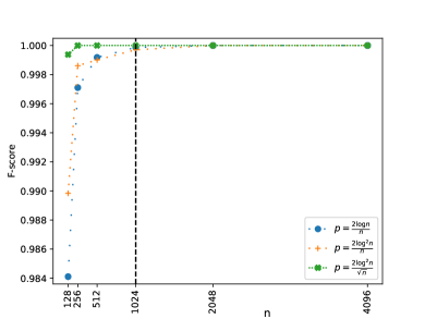
Figure 2: Community detection accuracy of CDRW algorithm on $G_{np}$ random graphs. It shows even when the graph is sparse, when $p$ is small and as close to the connectivity threshold as possible, its accuracy is still high. The vertical line shows that when the size is big enough ($n\geq 2^{10}$), the accuracy becomes almost $1.0$.

The first challenge for any community detection (CD) algorithm is detecting a random graph as a single community. This challenge becomes harder when the graph becomes sparse and it gets closer to the connectivity threshold of a random graph (i.e. $p=\frac{c\log n}{n}$, s.t. $c>1$) [7]. In the first experiment we show that our CDRW algorithm detects almost the whole graph as a single community resulting in a high F-score accuracy value, see Figure 2. Figure 2 shows that when we increase the size of graph $n$, the accuracy of our algorithm increases as well. For example, for $n=2^{10}$ the accuracy metric becomes almost $1.0$, meaning that almost all the nodes of the graph is detected as a single community. It also shows that when $p$ increases (graph gets denser), the accuracy also increases. So in the remaining experiments on PPM graphs, we choose two lowest values of $p=\frac{c\log n}{n}$ and $p=\frac{c\log^{2}{n}}{n}$ for generating its random parts in order to give more challenging input graphs to the CDRW algorithm.

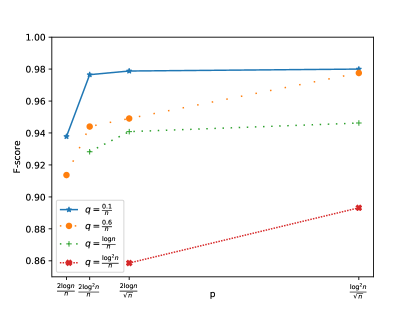
Figure 3: Performance of CDRW algorithm on PPM graphs when there are two parts/communities ($r=2$). We fixed the size of the graph to $n=2^{11}$, each planted partition is of size $2^{10}$. It shows that CDRW works well for small values of $p=\frac{2\log n}{n}$ and $p=\frac{2\log^{2}{n}}{n}$ when $q$ is small enough.

After showing that CDRW works well on $G_{np}$ random graphs, now we consider PPM $G_{npq}$ graphs. At first we fix the number of communities to two ($r=2$) so that we can consider the effect of various values of $p$ and $q$. This will show us the threshold for the ratio of $\frac{p}{q}$ where CDRW works well. As we showed in Figure 2, when the size of each random graph is big enough ($n\geq 2^{10}$), CDRW detects a single $G_{np}$ community well. Therefore we set the size of $G_{npq}$ to $n=2^{11}$ which makes each ground-truth community big enough ($\frac{n}{r}=2^{10}$). When considering PPM graphs with $p$ and $q$, as the connectivity probability for intra- and inter-community edges, CD algorithms face hardship in detecting communities when $p$ is small and $q$ is relatively high. But the $\frac{p}{q}$ ratio can not be arbitrarily small because it causes the two communities blend into each other and the graph looses its community structure. Figure 3 shows accuracy of CDRW for different values of $p$ and $q$. We highlight that it shows even for sparse parted $G_{npq}$ graphs: for $p=\frac{2\log n}{n}$, CDRW detects the two communities with a high F-score value (more than $0.90$) for $q=\frac{0.1}{n}$ and $\frac{0.6}{n}$. In other words, our CDRW algorithm works well even on sparse parted PPM graphs when the $\frac{p}{q}$ ratio is as small as ($\Omega(\log n)$). Notice that when $p=\frac{2\log n}{n}$, the two ground truth communities of the PPM graph are as sparse as possible, i.e close to its connectivity threshold. In the latter example, for instance, when $q=\frac{0.6}{n}$, a partition has in expectation $e_{in}=\binom{\frac{n}{r}}{2}p=10230$ intra and $e_{out}=\frac{n}{r}(n-\frac{n}{r})q=614$ inter community edges. It means the ratio of inter to intra community edges ($\frac{e_{out}}{e_{in}}$) is high and equal to $6\%$.

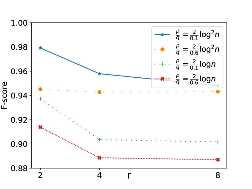
(a) $n=r\times 2^{10}$.

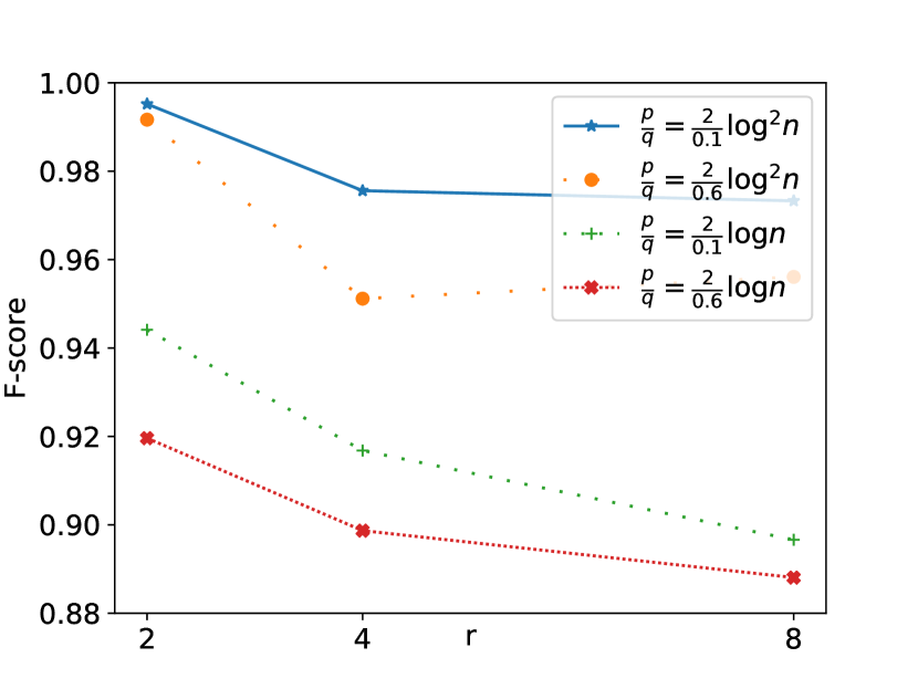
(b) $n=8\times 2^{10}$.

Figure 4: Varying the number of ground-truth communities to see its effect on the accuracy of our CDRW algorithm. It shows that when we increase the number of communities, the accuracy decreases slightly. This is expected because the number of inter-community edges increases. Comparing Sub-figure 4(a) and 4(b), we see that if we fix the number of communities, then the accuracy gets higher when the size of the communities becomes larger.

We now consider the effect of increasing the number of ground-truth communities ($r$) in order to see its effect on the accuracy of our CDRW algorithm, see Figure 4. We do it in two ways. First, we fix the size of each community to $2^{10}$ and vary the number of communities. The size of graph is $n=r\times 2^{10}$. Figure 4(a) shows that our CDRW algorithm works well when we reasonably increase the number of communities. Second, we fix the size of graph to a number so that the size of each community is $2^{10}$ when the number of communities is the biggest ($r=8$), see Figure 4(b). Then, when the number of communities becomes lower, the size of communities gets bigger. By comparing Sub-figures 4(a) and 4(b), we see that when the number of communities are the same, the accuracy is higher when the size of each community is bigger.

V Conclusion

We proposed a distributed algorithm, CDRW, for community detection that works well for the PPM model ($G_{npq}$ random graph), a standard random graph model used extensively in clustering and community detection studies. Our CDRW algorithm is relatively simple and localized; it uses random walk and mixing time property of graphs to detect communities. We provide a rigorous theoretical analysis of our algorithm on the $G_{npq}$ random graph and characterize its performance vis-a-vis the parameters of the model. In particular, our main result is that it correctly identifies the communities provided $q=o(p/(r\log(n/r)))$, where $r$ is the number of communities. Our algorithm takes $O(r\times\mbox{polylog }n)$ rounds and hence is quite fast when $r$ is relatively small. We point out that our algorithm can also be extended to find communities even faster (by finding communities in parallel), assuming we know an (estimate) of $r$. For future work, it will be interesting to study the performance of this algorithm on other graph models and can be a starting point to design and analyze community detection algorithms that perform well in the more challenging case of real-world graphs.

References

- [1] E. Abbe. Community detection and stochastic block models: Recent developments. Journal of Machine Learning Research, 18(177):1–86, 2018.
- [2] E. Abbe and C. Sandon. Community detection in general stochastic block models: Fundamental limits and efficient algorithms for recovery. In Foundations of Computer Science (FOCS), 2015 IEEE 56th Annual Symposium on, pages 670–688. IEEE, 2015.
- [3] S. Bandyapadhyay, T. Inamdar, S. Pai, and S. V. Pemmaraju. Near-optimal clustering in the -machine model. In Proceedings of the 19th International Conference on Distributed Computing and Networking (ICDCN), 2018.
- [4] L. Becchetti, A. Clementi, E. Natale, F. Pasquale, and L. Trevisan. Find your place: Simple distributed algorithms for community detection. In Proceedings of the Twenty-Eighth Annual ACM-SIAM Symposium on Discrete Algorithms, pages 940–959. SIAM, 2017.
- [5] L. Becchetti, A. E. F. Clementi, P. Manurangsi, E. Natale, F. Pasquale, P. Raghavendra, and L. Trevisan. Average whenever you meet: Opportunistic protocols for community detection. In Y. Azar, H. Bast, and G. Herman, editors, 26th Annual European Symposium on Algorithms, ESA 2018, August 20-22, 2018, Helsinki, Finland, volume 112 of LIPIcs, pages 7:1–7:13. Schloss Dagstuhl - Leibniz-Zentrum fuer Informatik, 2018.
- [6] F. Bénézit, P. Thiran, and M. Vetterli. Interval consensus: from quantized gossip to voting. In Acoustics, Speech and Signal Processing, 2009. ICASSP 2009. IEEE International Conference on, pages 3661–3664. IEEE, 2009.
- [7] B. Bollobás. Random graphs. In Modern graph theory, pages 215–252. Springer, 1998.
- [8] P. Chin, A. Rao, and V. Vu. Stochastic block model and community detection in sparse graphs: A spectral algorithm with optimal rate of recovery. In Conference on Learning Theory, pages 391–423, 2015.
- [9] F. Chung and L. Lu. The diameter of sparse random graphs. Advances in Applied Mathematics, 26(4):257–279, 2001.
- [10] A. Clementi, M. Di Ianni, G. Gambosi, E. Natale, and R. Silvestri. Distributed community detection in dynamic graphs. Theoretical Computer Science, 584:19–41, 2015.
- [11] A. Condon and R. M. Karp. Algorithms for graph partitioning on the planted partition model. In Randomization, Approximation, and Combinatorial Optimization. Algorithms and Techniques, pages 221–232. Springer, 1999.
- [12] A. Condon and R. M. Karp. Algorithms for graph partitioning on the planted partition model. Random Structures & Algorithms, 18(2):116–140, 2001.
- [13] W. Donath and A. Hoffman. Algorithms for partitioning of graphs and computer logic based on eigenvectors of connections matrices. IBM Technical Disclosure Bulletin, 15, 1972.
- [14] M. E. Dyer and A. M. Frieze. The solution of some random np-hard problems in polynomial expected time. Journal of Algorithms, 10(4):451–489, 1989.
- [15] D. Easley and J. Kleinberg. Networks, crowds, and markets: Reasoning about a highly connected world. Cambridge University Press, 2010.
- [16] P. Erdős and A. Rényi. On the evolution of random graphs. Publ. Math. Inst. Hung. Acad. Sci, 5:17–61, 1960.
- [17] S. Fortunato. Community detection in graphs. Physics reports, 486(3-5):75–174, 2010.
- [18] S. Fortunato and D. Hric. Community detection in networks: A user guide. Physics Reports, 659:1–44, 2016.
- [19] J. Friedman. A proof of Alon’s second eigenvalue conjecture and related problems. American Mathematical Society, Providence, RI, USA, 2008.
- [20] M. Girvan and M. E. Newman. Community structure in social and biological networks. Proceedings of the national academy of sciences, 99(12):7821–7826, 2002.
- [21] P. W. Holland, K. B. Laskey, and S. Leinhardt. Stochastic blockmodels: First steps. Social networks, 5(2):109–137, 1983.
- [22] S. Hoory, N. Linial, and A. Wigderson. Expander graphs and their applications. Bulletin of the American Mathematical Society, 43(4):439–561, 2006.
- [23] T. Inamdar, S. Pai, and S. V. Pemmaraju. Large-scale distributed algorithms for facility location with outliers. In The 22nd International Conference on Principles of Distributed Systems (OPODIS), 2018.
- [24] H. J. Karloff, S. Suri, and S. Vassilvitskii. A model of computation for MapReduce. In Proceedings of the 21st annual ACM-SIAM Symposium on Discrete Algorithms (SODA), pages 938–948, 2010.
- [25] B. Karrer and M. E. Newman. Stochastic blockmodels and community structure in networks. Physical review E, 83(1):016107, 2011.
- [26] H. Klauck, D. Nanongkai, G. Pandurangan, and P. Robinson. Distributed computation of large-scale graph problems. In Proceedings of the 26th Annual ACM-SIAM Symposium on Discrete Algorithms (SODA), pages 391–410, 2015.
- [27] K. Kothapalli, S. V. Pemmaraju, and V. Sardeshmukh. On the analysis of a label propagation algorithm for community detection. In International Conference on Distributed Computing and Networking, pages 255–269. Springer, 2013.
- [28] F. Kuhn and A. R. Molla. Distributed sparse cut approximation. In OPODIS, 2015.
- [29] J. Lei, A. Rinaldo, et al. Consistency of spectral clustering in stochastic block models. The Annals of Statistics, 43(1):215–237, 2015.
- [30] L. Lovász. Random walks on graphs: A survey. Combinatorics, 2:1–46, 1993.
- [31] G. Malewicz, M. H. Austern, A. J. C. Bik, J. C. Dehnert, I. Horn, N. Leiser, and G. Czajkowski. Pregel: a system for large-scale graph processing. In Proceedings of the 2010 ACM International Conference on Management of Data (SIGMOD), pages 135–146, 2010.
- [32] C. D. Manning, P. Raghavan, and H. Schütze. Introduction to Information Retrieval. Cambridge University Press, New York, NY, USA, 2008.
- [33] A. R. Molla and G. Pandurangan. Local mixing time: Distributed computation and applications. In Proc. of 32nd IEEE International Parallel and Distributed Processing Symposium (IPDPS), pages 743–752, 2018.
- [34] E. Mossel, J. Neeman, and A. Sly. Stochastic block models and reconstruction. arXiv preprint arXiv:1202.1499, 2012.
- [35] M. E. Newman and M. Girvan. Finding and evaluating community structure in networks. Physical review E, 69(2):026113, 2004.
- [36] A. Olshevsky and J. N. Tsitsiklis. Convergence speed in distributed consensus and averaging. SIAM review, 53(4):747–772, 2011.
- [37] G. Pandurangan. Distributed Network Algorithms. url: https://sites.google.com/site/gopalpandurangan/dna, 2016.
- [38] G. Pandurangan, P. Robinson, and M. Scquizzato. Fast distributed algorithms for connectivity and MST in large graphs. In Proceedings of the 28th ACM Symposium on Parallelism in Algorithms and Architectures, SPAA, pages 429–438, 2016.
- [39] G. Pandurangan, P. Robinson, and M. Scquizzato. On the distributed complexity of large-scale graph computations. In Proceedings of the 30th ACM Symposium on Parallelism in Algorithms and Architectures (SPAA), pages 405–414, 2018.
- [40] D. Peleg. Distributed computing: a locality-sensitive approach. SIAM, Philadelphia, PA, USA, 2000.
- [41] R. Peng, H. Sun, and L. Zanetti. Partitioning well-clustered graphs: Spectral clustering works! In Conference on Learning Theory, pages 1423–1455, 2015.
- [42] P. Pons and M. Latapy. Computing communities in large networks using random walks. J. Graph Algorithms Appl., 10(2):191–218, 2006.
- [43] U. N. Raghavan, R. Albert, and S. Kumara. Near linear time algorithm to detect community structures in large-scale networks. Physical review E, 76(3):036106, 2007.
- [44] D. A. Reed and J. Dongarra. Exascale computing and big data. Commun. ACM, 58(7):56–68, 2015.
- [45] D. Shah et al. Gossip algorithms. Foundations and Trends® in Networking, 3(1):1–125, 2009.
- [46] H. Zhou and R. Lipowsky. Network brownian motion: A new method to measure vertex-vertex proximity and to identify communities and subcommunities. In International conference on computational science, pages 1062–1069. Springer, 2004.