Diffusion-reaction model for positron trapping and annihilation at spherical extended defects and in precipitate$-$matrix composites

Abstract

The exact solution of a diffusion$-$reaction model for the trapping and annihilation of positrons in small extended spherical defects (clusters, voids, small precipitates) with competitive rate-limited trapping in vacancy-type point defects is presented. Closed-form expressions are obtained for the mean positron lifetime and for the intensities of the two positron lifetime components associated with trapping at defects. The exact solutions can be conveniently applied for the analysis of experimental data and allow an assessment in how far the usual approach, which takes diffusion limitation into account by means of effective diffusion-trapping rates, is appropriate. The model is further extended for application to larger precipitates where diffusion- and reaction limited trapping is not only considered for the trapping from the matrix into the precipitate$-$matrix interface but also for the trapping from inside the precipitates into the interfaces. This makes the model applicable to all type of composite structures where spherical objects are embedded in a matrix irrespective of their size and their number density.

I Introduction

The versatile technique of positron annihilation makes use of the fact that positrons ($e^{+}$) are trapped at free volume-type defects which allows their detection by a specific variation of the positron-electron annihilation characteristics Hautojärvi (1979); Keeble et al. (2012); Krause-Rehberg and Leipner (1999); Puska and Nieminen (1994). Whereas the kinetics of $e^{+}$ trapping at vacancy-type point defects can be well described by rate theory (so-called simple trapping model), it is well known that for trapping at extended defects like grain boundaries, interfaces, voids, clusters, or precipitates, diffusion limitation of the trapping process may be an issue. Diffusion-limited positron trapping at interfaces and grain boundaries has been quantatively modeled by several groups, ranging from entirely diffusion-controlled trapping Brandt and Paulin (1972), diffusion-reaction controlled trapping including detrapping Dupasquier et al. (1993); Würschum and Seeger (1996); Kögel (1996); Dryzek (1999), up to diffusion-reaction controlled trapping at grain boundaries and competetive transition-limited trapping at point defects in crystals C̆iz̆ek et al. (2002); Oberdorfer and Würschum (2009); Dryzek et al. (1998); Kögel (1996).

Compared to grain boundaries, diffusion-limited $e^{+}$ trapping at voids and clusters has not been studied in such detail despite the undoubted relevance of positron annihilation for studying this important class of defects Nieminen and Laakkonen (1979); Bentzon and Evans (1990); Eldrup and Singh (2003). One approach to deal with diffusion-limited trapping is based on effective diffusion-trapping rates which then allow an implementation in standard rate theory (e.g., Bentzon and Evans (1990)). Diffusion-limited trapping at point-like defects was studied by Dryzek Dryzek (1998) for the one-dimensional case. A full treatment of $e^{+}$ trapping and annihilation in voids in the framework of diffusion-reaction theory was given by Nieminen et al. Nieminen et al. (1979). This treatment of Nieminen et al. Nieminen et al. (1979) is conceptionally analogous to the subsequent work of Dupasquier et al. Dupasquier et al. (1993) for diffusion-limited $e^{+}$ trapping at grain boundaries, both of which lead to solutions exclusively in terms of infinite series.

Another treatment of the diffusion-reaction problem of $e^{+}$ trapping at grain boundaries was given by Würschum and Seeger Würschum and Seeger (1996) which yields closed-form expressions for the mean $e^{+}$ lifetime and the intensity of the annihilation component associated with the trapped state. This approach is applied in the present work to the diffusion-reaction problem of $e^{+}$ trapping and annihilation in spherical extended defects (voids, clusters, precipitates). Following our earlier further work on grain boundaries Oberdorfer and Würschum (2009), now in addition competitive reaction rate-limiting trapping at point defects is taken into account. The present treatment yields closed-form expressions of the major $e^{+}$ annihilation parameters for this application-relevant case of competitive $e^{+}$ trapping in voids and point defects. These closed-form expressions allow deeper insight in the physical details of $e^{+}$ annihilation characteristics as well as an assessment of the so far often used approach based on effective diffusion-trapping rates. Above all, the results can be conveniently applied for the analysis of experimental data.

In a further part, the model presented here and the previous model on positron trapping at grain boundaries are merged in order to study precipitates embedded in matrix. Here, diffusion- and reaction limited trapping is considered for both the trapping from the matrix into the precipitate$-$matrix interface and for the trapping from inside the precipitates into the interfaces.

II The Model

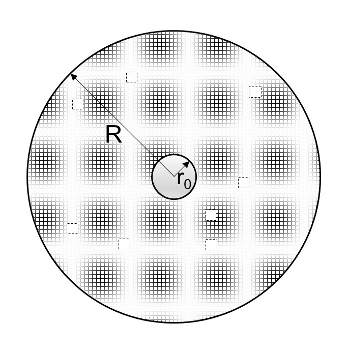
Figure 1: Geometry of the diffusion-reaction model: spherical voids of radius $r_{0}$ are located in a lattice with homogeneously distributed vacancy-type defects ($\Box$) in which reaction-controlled trapping occurs. The outer radius $R$ of the diffusion sphere defines the void concentration.

The model describes positron ($e^{+}$) trapping and annihilation in voids in the general case that both the $e^{+}$ diffusion and the transition reaction has to be taken into account (so called diffusion-reaction controlled trapping process). In order to cover more complex cases, competitive transition-limited trapping at vacancy-type points defects is also considered (see Fig. 1). This procedure follows our earlier study where concomitant positron trapping at grain boundaries and at point defects in crystallites has been considered Oberdorfer and Würschum (2009).

The behavior of the positrons is described by their bulk (free) lifetime $\tau_{f}$, by their lifetime ($\tau_{t})$ in the voids, by their lifetime ($\tau_{v})$ in the vacancy-type point defects in the lattice (matrix), and by their bulk diffusivity $D$. Trapping at the point defects of the matrix is characterized by the specific $e^{+}$ trapping rate $\sigma_{v}$ (unit s^-1), as usual. The voids are considered as spherical-shaped extended defects (radius $r_{0}$) with a specific trapping rate $\alpha$ (unit m s^-1) which is related to the surface area of the void. In units of s^-1 the specific trapping rate of voids reads

$$\sigma_{t}=\frac{\alpha 4\pi r_{0}^{2}}{\Omega},$$ (1)

where $\Omega$ denotes the atomic volume.

The temporal and spatial evolution of the density $\rho_{l}$ of free positrons in the lattice is governed by:

$$\frac{\partial\rho_{l}}{\partial t}=D\nabla^{2}\rho_{l}-\rho_{l}\left(\frac{1}{\tau_{f}}+\sigma_{v}C_{v}\right)$$ (2)

where $C_{v}$ denotes the concentration of vacancy-type point defects in the matrix. The positrons trapped in the voids are described in terms of their density $\rho_{t}$ obeying the rate equation

$$\frac{\mathrm{d}\rho_{t}}{\mathrm{d}t}=\alpha\rho_{l}(r_{0},t)-\frac{1}{\tau_{t}}\rho_{t}.$$ (3)

The temporal evolution of the number $N_{v}$ of $e^{+}$ trapped in the point defects in the lattice is given by

$$\frac{\mathrm{d}N_{v}}{\mathrm{d}t}=-\frac{1}{\tau_{v}}N_{v}+\sigma_{v}C_{v}N_{f}\,,$$ (4)

where the number $N_{f}$ of positrons in the free state follows from integration of $\rho_{l}$:

$$N_{f}=\int\rho_{l}\mathrm{d}V.$$ (5)

The continuity of the ${\rm e}^{+}$ flux at the boundary between the lattice and the void surface is expressed by

$$D\nabla\rho_{l}\Big{|}_{r=r_{0}}-\alpha\rho_{l}(r_{0},t)=0.$$ (6)

The outer radius $R$ of the diffusion sphere is related to the void concentration

$$C_{t}=\frac{3\Omega}{4\pi R^{3}}\,.$$ (7)

The outer boundary condition

$$\frac{\partial\rho_{l}}{\partial r}\Big{|}_{r=R}=0$$ (8)

reflects the vanishing $e^{+}$ flux through the outer border ($r=R$) of the diffusion sphere. This boundary condition is the same as applied earlier in a quite different diffusion-reaction model of ortho-para conversion of positronium at reaction cerntres Würschum and Seeger (1995).

As initial condition we adopt the picture that at $t=0$ all thermalized positrons are in the free state and homogeneously distributed in the lattice, i.e., initial density $\rho_{l}=\rho_{l}(0)$, $\rho_{t}(0)=0$, $N_{v}(0)=0$. Under this initial condition the solution of Eq. (2) exhibits spherical symmetry.

Up to this point the above formulated diffusion-reaction problem is identical to that of Nieminen et al. Nieminen et al. (1979) apart from the additional rate-limited trapping at vacancy-type point defects which is considered here. However, compared to Nieminen et al. (1979), in the following part of the present work the time dependence is handled by means of Laplace transformation which will lead to the more convenient closed-form solutions. Applying the Laplace transformation

$$\tilde{\rho}_{l,t}(p)=\int\limits_{0}^{\infty}\exp(-pt)\rho_{l,t}(t)\mathrm{d}t,$$

$$\tilde{N}_{v,f}(p)=\intop_{0}^{\infty}\exp(-pt)N_{v,f}(t)\mathrm{d}t$$ (9)

leads to the basic equations

$$\frac{\mathrm{d^{2}}\tilde{\rho}_{l}}{\mathrm{d}r^{2}}+\frac{2}{r}\frac{\mathrm{d}\tilde{\rho}_{l}}{\mathrm{d}r}-\gamma^{2}\tilde{\rho}_{l}=-\frac{\rho_{l}(0)}{D}$$ (10)

with

$$\gamma^{2}=\gamma^{2}(p)=\frac{\tau_{f}^{-1}+\sigma_{v}C_{v}+p}{D}\,,$$ (11)

and

$$\tilde{\rho}_{t}=\frac{\alpha\tilde{\rho}_{l}(r_{0},p)}{\tau_{t}^{-1}+p}\>,$$ (12)

$$\tilde{N}_{v}=\frac{\sigma_{v}C_{v}}{\tau_{v}^{-1}+p}\times\int\limits^{R}_{r_{0}}4\pi r^{2}\tilde{\rho_{l}}(r,p){\rm d}r\>,$$ (13)

with the boundary conditions

$$D\,\frac{\mathrm{d}\tilde{\rho}_{l}}{\mathrm{d}r}\Bigg{|}_{r=r_{0}}-\alpha\tilde{\rho}_{l}(r_{0},p)=0$$ (14)

and

$$\frac{\mathrm{d}\tilde{\rho}_{l}}{\mathrm{d}r}\Bigg{|}_{r=R}=0\,.$$ (15)

The solution of the differential equation (10) satisfying equations [Eq. (14)] and [Eq. (15)] can be written as

$$\tilde{\rho}_{l}(r,p)=A\,i_{0}^{(1)}(\gamma r)+B\,i_{0}^{(2)}(\gamma r)+\frac{\rho_{l}(0)}{\tau_{f}^{-1}+\sigma_{v}C_{v}+p}$$ (16)

with

$$A:= \displaystyle{\alpha~{}\frac{\rho_{l}(0)}{\tau_{f}^{-1}+\sigma_{v}C_{v}+p}~{}\times~{}\frac{i_{1}^{(2)}(\gamma R)}{-D\gamma F_{1}+\alpha F_{2}}}\,,$$

$$B:= \displaystyle{\alpha~{}\frac{\rho_{l}(0)}{\tau_{f}^{-1}+\sigma_{v}C_{v}+p}~{}\times~{}\frac{i_{1}^{(1)}(\gamma R)}{D\gamma F_{1}-\alpha F_{2}}}$$ (17)

and

$$F1=i_{1}^{(2)}(\gamma r_{0})i_{1}^{(1)}(\gamma R)-i_{1}^{(1)}(\gamma r_{0})i_{1}^{(2)}(\gamma R)\,,$$

$$F2=i_{0}^{(2)}(\gamma r_{0})i_{1}^{(1)}(\gamma R)-i_{0}^{(1)}(\gamma r_{0})i_{1}^{(2)}(\gamma R)\,.$$ (18)

$i_{n}^{(1)}$ and $i_{n}^{(2)}$ ($n=0,1$) denote the modified spherical Bessel functions of order $n$ Olver (2010)

$$i_{n}^{(1)}(z):=(\frac{\pi}{2z})^{1/2}I_{n+1/2}(z),\,$$

$$i_{0}^{(1)}=\frac{\sinh z}{z},\quad i_{1}^{(1)}=\frac{\cosh z}{z}-\frac{\sinh z}{z^{2}}$$ (19)

$$i_{n}^{(2)}(z):=(\frac{\pi}{2z})^{1/2}I_{-n-1/2}(z),\,$$

$$i_{0}^{(2)}=\frac{\cosh z}{z},\quad i_{1}^{(2)}=\frac{\sinh z}{z}-\frac{\cosh z}{z^{2}}$$ (20)

where $I_{\pm n\pm 1/2}(z)$ represents the Bessel function.

Basis for analyzing positron annihilation experiments is the total probability $n(t)$ that a $e^{+}$ implanted at $t=0$ has not yet been annihilated at time $t$. Here $n(t)$ is given by the number density of $e^{+}$ per lattice sphere at time $t$:

$$n(t)=\frac{1}{\frac{4}{3}\pi(R^{3}-r_{0}^{3})\rho_{l}(0)}\times\left\{\int\limits_{r_{0}}^{R}4\pi r^{2}\rho_{l}(r,t)\mathrm{d}r+4\pi r_{0}^{2}\rho_{t}(t)+N_{v}(t)\right\}\>.$$ (21)

The Laplace transform of $n(t)$ can be calculated taking into account the solution of $\tilde{N}_{v}$ [Eq. (13)] and the solution of the differential equation (16) which yields

$$\tilde{n}(p)=\frac{1}{\frac{4}{3}\pi(R^{3}-r_{0}^{3})\rho_{l}(0)}\times\left\{\left(1+\frac{\sigma_{v}C_{v}}{\tau_{v}^{-1}+p}\right)\int\limits^{R}_{r_{0}}4\pi r^{2}\tilde{\rho}_{l}(r,p){\rm d}r+4\pi r^{2}_{0}\tilde{\rho}_{t}(p)\right\}\>.$$ (22)

Solving the integral after substituting $\tilde{\rho_{t}}(p)$ by Eq. (12), insertion of $A$ and $B$ [Eq. (17)], yields after some algebra

$$\tilde{n}(p)=\frac{1}{t_{fc}^{2}t_{v}t_{t}}\Biggl{\{}t_{vc}t_{fc}t_{t}+\frac{K(t_{fc}t_{v}-t_{vc}t_{t})\Bigl{(}\gamma\hat{R}-\tanh(\gamma\hat{R})[1-\gamma^{2}r_{0}R]\Bigr{)}}{\gamma\hat{R}-\tanh(\gamma\hat{R})[1-\gamma^{2}r_{0}R]+\frac{\alpha r_{0}}{D}[\gamma R-\tanh(\gamma\hat{R})]}\Biggr{\}}$$ (23)

with

$$K=\frac{3\alpha r_{0}^{2}}{R^{3}-r_{0}^{3}}\,,$$ (24)

$$\hat{R}=R-r_{0}\,,$$ (25)

and the abbreviations

$$t_{t}=\tau_{t}^{-1}+p\,; t_{v}=\tau_{v}^{-1}+p\,;$$

$$t_{vc}=\tau_{v}^{-1}+\sigma C+p\,; t_{fc}=\tau_{f}^{-1}+\sigma C+p\,.$$ (26)

The Laplace transform $\tilde{n}(p)$ [Eq. (23)] represents the solution of the present diffusion and trapping model from which both the mean positron lifetime and the positron lifetime spectrum can be deduced. The mean positron lifetime $\overline{\tau}$ is obtained by taking the Laplace transform at $p=0$:

$$\overline{\tau}=\tilde{n}(p=0)=\int\limits^{\infty}_{0}n(t)dt\,.$$ (27)

The positron lifetime spectrum follows from $\tilde{n}(p)$ by means of Laplace inversion. The single poles $p=-\lambda_{i}$ of $\tilde{n}(p)$ in the complex $p$ plane define the decay rates $\lambda_{i}(i=0,1,2,\dots)$ of the positron lifetime spectrum:

$$n(t)=\sum_{i=0}^{\infty}I_{i}\exp(-\lambda_{i}t)\,,$$ (28)

where $I_{i}$ denote the relative intensities.

III Analysis

At first, we consider the most important case that $e^{+}$ trapping exclusively occurs at voids, i.e., we omit $e^{+}$ trapping at point defects in the lattice ($C_{v}=0$). For this case, we present the solution of the general diffusion-reaction theory (Sect. III.1) and compare it with the limiting cases of entirely reaction-controlled trapping (Sect. III.2) and entirely diffusion-controlled trapping (Sect. III.3). Finally, the case of competitive reaction-controlled trapping at lattice defects is considered (Sect. III.4) and an extension to larger precipitates is presented for describing precipitate$-$matrix composite structures (Sect. III.5).

III.1 General case with trapping at voids, exclusively ($C_{v}=0$)

For negligible trapping at vacancies within the lattice ($C_{v}=0$), the diffusion-reaction model according to Eq. (23) yields for positron trapping in voids as the single type of trap:

$$\tilde{n}(p)=\frac{1}{\tau_{f}^{-1}+p}\Biggl{\{}1+\frac{K(\tau_{f}^{-1}-\tau_{t}^{-1})}{(\tau_{t}^{-1}+p)(\tau_{f}^{-1}+p)}\times\frac{\gamma\hat{R}-\tanh(\gamma\hat{R})[1-\gamma^{2}r_{0}R]}{\gamma\hat{R}-\tanh(\gamma\hat{R})[1-\gamma^{2}r_{0}R]+\frac{\alpha r_{0}}{D}[\gamma R-\tanh(\gamma\hat{R})]}\Biggr{\}}$$ (29)

and, hence, for the mean positron lifetime

$$\overline{\tau}=\tilde{n}(0)=\tau_{f}\Biggl{\{}1+K(\tau_{t}-\tau_{f})\times\frac{\gamma_{0}\hat{R}-\tanh(\gamma_{0}\hat{R})[1-\gamma_{0}^{2}r_{0}R]}{\gamma_{0}\hat{R}-\tanh(\gamma_{0}\hat{R})[1-\gamma_{0}^{2}r_{0}R]+\frac{\alpha r_{0}}{D}[\gamma_{0}R-\tanh(\gamma_{0}\hat{R})]}\Biggr{\}}\,.$$ (30)

The pole of Eq. (29) for $p=-\tau_{t}^{-1}$ corresponds to the positron lifetime component $\tau_{t}$ of the void-trapped state for which the following intensity is obtained:

$$I_{t}=\frac{K}{\tau_{f}^{-1}-\tau_{t}^{-1}}\times\frac{\gamma_{t}\hat{R}-\tanh(\gamma_{t}\hat{R})[1-\gamma_{t}^{2}r_{0}R]}{\gamma_{t}\hat{R}-\tanh(\gamma_{t}\hat{R})[1-\gamma_{t}^{2}r_{0}R]+\frac{\alpha r_{0}}{D}[\gamma_{t}R-\tanh(\gamma_{t}\hat{R})]}\,.$$ (31)

In equations (29), (30), (31):

$$\gamma^{2}=\frac{\tau_{f}^{-1}+p}{D};\,\gamma_{0}^{2}=\frac{\tau_{f}^{-1}}{D};\,\gamma_{t}^{2}=\frac{\tau_{f}^{-1}-\tau_{t}^{-1}}{D}\,.$$ (32)

In addition to the annihilation component $\tau_{t}^{-1}$ of the void-trapped state, $\tilde{n}(p)$ [Eq. (29)] comprises a sequence of first-order poles $p=-\lambda_{0,j}$ for $\lambda_{0,j}>\tau_{f}^{-1}$. These components $\lambda_{0,j}$, which define the fast decay rates ($\lambda_{0,j}>\tau_{f}^{-1}$) of the $e^{+}$ lifetime spectrum, are given by the solutions of the transcendental equation

$$\tan(\gamma^{\star}\hat{R})=\frac{\gamma^{\star}(\alpha r_{0}R+D\hat{R})}{D(1+\gamma^{\star 2}r_{0}R)+\alpha r_{0}}$$ (33)

with

$$\gamma^{\star 2}=\frac{\lambda_{0,j}-\tau_{f}^{-1}}{D}$$ (34)

in agreement with the aforementioned earlier work of Nieminen et al. Nieminen et al. (1979).^, As usual for this kind of diffusion-reaction problem (see, e.g. Oberdorfer and Würschum (2009)), the intensities of these decay rates rapidly decrease. Experimentally only a single fast decay rate can be resolved in addition to the decay rate $\tau_{t}^{-1}$ of the trapped state. An experimental two-component $e^{+}$ lifetime spectrum is practically entirely defined by $\overline{\tau}$ [Eq. (30)] and by $\tau_{t}$ with the corresponding intensity $I_{t}$ [Eq. (31)].

The appearance of a second-order pole in Eq. (29) at $p=-\tau_{f}^{-1}$ (i.e., $\gamma=0$) is spurious. Closer inspection by applying Taylor expansion shows that the intensity associated with this pole cancels.

Following the consideration of Dryzek Dryzek (2002), in analogy to the mean $e^{+}$ lifetime [Eq. (30)] a respective relation for the mean line shape parameter $\overline{S}$ of Doppler broadening of the positron-electron annihilation can be given:

$$\overline{S}=S_{f}\Biggl{\{}1+K(S_{t}-S_{f})\times\frac{\gamma_{0}\hat{R}-\tanh(\gamma_{0}\hat{R})[1-\gamma_{0}^{2}r_{0}R]}{\gamma_{0}\hat{R}-\tanh(\gamma_{0}\hat{R})[1-\gamma_{0}^{2}r_{0}R]+\frac{\alpha r_{0}}{D}[\gamma_{0}R-\tanh(\gamma_{0}\hat{R})]}\Biggr{\}}\,,$$ (35)

where $S_{f}$ and $S_{t}$ denote the line shape parameters of the free and trapped state, respectively.

For the sake of completeness, we quote $\tilde{n}(p)$ without derivation for the case that at time zero positrons are homogeneously distributed in the voids and the lattice, i.e., for the initial condition $\rho_{t}(0)=r_{0}\rho_{l}(0)/3$:

$$\tilde{n}(p)=\displaystyle{\frac{1}{\tau_{f}^{-1}+p}\Biggl{\{}1+\frac{r_{0}^{3}}{R^{3}}\times\frac{\tau_{f}^{-1}-\tau_{t}^{-1}}{\tau_{t}^{-1}+p}+}\frac{3\alpha r_{0}^{2}}{R^{3}}\times\frac{\tau_{f}^{-1}-\tau_{t}^{-1}}{(\tau_{t}^{-1}+p)(\tau_{f}^{-1}+p)}\times$$

$$\displaystyle{\frac{\gamma\hat{R}-\tanh(\gamma\hat{R})[1-\gamma^{2}r_{0}R]}{\gamma\hat{R}-\tanh(\gamma\hat{R})[1-\gamma^{2}r_{0}R]+\frac{\alpha r_{0}}{D}[\gamma R-\tanh(\gamma\hat{R})]}\Biggr{\}}}\,.$$ (36)

Eq. (III.1) includes in the limiting case of negligible trapping ($\alpha=0$) as mean $e^{+}$ lifetime $\overline{\tau}=\tilde{n}(0)=[(R^{3}-r_{0}^{3})\tau_{f}+r_{0}^{3}\tau_{t}]/R^{3}$ the expected volume-averaged mean value of $\tau_{f}$ and $\tau_{t}$.

III.2 Limiting case of entirely reaction limited trapping ($C_{v}=0$)

If the e⁺ diffusivity is high ($\gamma\hat{R}\ll 1$), the hyperbolic tangent in Eq. (29) can be expanded. Expansion up to the third order

$$\tanh(z)\approx z-\frac{z^{3}}{3}$$ (37)

yields the mean $e^{+}$ lifetime

$$\overline{\tau}=\displaystyle{\tau_{f}\frac{1+K\tau_{t}}{1+K\tau_{f}}}$$ (38)

and for the $e^{+}$ lifetime component $\tau_{t}$ the intensity

$$I_{t}=\displaystyle{\frac{K}{\tau_{f}^{-1}+K-\tau_{t}^{-1}}}$$ (39)

with $K$ according to Eq. (24). Equations (38) and (39) are the well-known solutions of the simple trapping model when we identify $K$ for vanishing defect volume with the trapping rate $\sigma_{t}C_{t}$ [equations (1) and (7)]. Note that the standard trapping model does not take into account the finite defect volume (here $4\pi r_{0}^{3}/3$) and, therefore, does not contain the subtrahend $r_{0}^{3}$ as in Eq. (24). With this subtrahend, equations (38) and (39) correctly contain the exact values $\overline{\tau}=\tau_{t}$ and $I_{t}=1$ as limiting case for $R=r_{0}$.

III.3 Limiting case of entirely diffusion limited trapping ($C_{v}=0$)

The present solution includes in the limiting special case $\alpha\rightarrow\infty$ the relationships for an entirely diffusion-limited trapping, i.e., for Smoluchowski-type boundary condition

$$\rho_{l}(r_{0},t)=0\,.$$ (40)

In this limit one obtains from the Laplace transform [Eq. (29)] the mean $e^{+}$ lifetime

$$\overline{\tau}=\tau_{f}\Biggl{\{}1+\frac{3r_{\rm 0}D}{R^{3}-r_{\rm 0}^{3}}(\tau_{t}-\tau_{f})\frac{\gamma_{0}\hat{R}-\tanh(\gamma_{0}\hat{R})[1-\gamma_{0}^{2}r_{0}R]}{\gamma_{0}R-\tanh(\gamma_{0}\hat{R})}\Biggr{\}}$$ (41)

and for the trap component $\tau_{t}$ the intensity

$$I_{t}=\frac{3r_{0}D}{R^{3}-r_{0}^{3}}\times\frac{1}{\tau_{f}^{-1}-\tau_{t}^{-1}}\times\frac{\gamma_{t}\hat{R}-\tanh(\gamma_{t}\hat{R})[1-\gamma_{t}^{2}r_{0}R]}{\gamma_{t}R-\tanh(\gamma_{t}\hat{R})}$$ (42)

with $\gamma_{0}$, $\gamma_{t}$ according to eq. (32).

III.4 General case with voids and lattice vacancies

The positron annihilation characteristics of diffusion-reaction controlled trapping at voids and concomitant transition-limited trapping at point defects in the lattice is given by Eq. (23) in combination with Eq. (27) and Eq. (28). The mean positron lifetime [Eq. 27], obtained from Eq. (23) for $p=0$, reads in the general case:

$$\overline{\tau}=\displaystyle{\frac{1}{(\tau_{f}^{-1}+\sigma_{v}C_{v})^{2}}}\Biggl{\{}(\tau_{f}^{-1}+\sigma_{v}C_{v})(\tau_{v}^{-1}+\sigma_{v}C_{v})\tau_{v}+$$

$$\displaystyle{\frac{K\Bigl{(}(\tau_{f}^{-1}+\sigma_{v}C_{v})\tau_{t}-(\tau_{v}^{-1}+\sigma_{v}C_{v})\tau_{v}\Bigr{)}\Bigl{(}\gamma_{0}\hat{R}-\tanh(\gamma_{0}\hat{R})[1-\gamma^{2}r_{0}R]\Bigr{)}}{\gamma_{0}\hat{R}-\tanh(\gamma_{0}\hat{R})[1-\gamma_{0}^{2}r_{0}R]+\frac{\alpha r_{0}}{D}[\gamma_{0}R-\tanh(\gamma_{0}\hat{R})]}\Biggr{\}}}$$ (43)

with

$$\gamma_{0}^{2}=\frac{\tau_{f}^{-1}+\sigma_{v}C_{v}}{D}\,.$$ (44)

In addition to the pole $p=-\tau_{t}^{-1}$ which characterizes the void trapped state, $\tilde{n}(p)$ [Eq. (23)] contains the further defect-related pole $p=-\tau_{v}^{-1}$ for the vacancy-type defect in the lattice. From the residues of $\tilde{n}(p)$ [Eq. (23)], the corresponding relative intensities

$$I_{t}=\frac{K}{\tau_{f}^{-1}+\sigma_{v}C_{v}-\tau_{t}^{-1}}\times\frac{\gamma_{t}\hat{R}-\tanh(\gamma_{t}\hat{R})[1-\gamma_{t}^{2}r_{0}R]}{\gamma_{t}\hat{R}-\tanh(\gamma_{t}\hat{R})[1-\gamma_{t}^{2}r_{0}R]+\frac{\alpha r_{0}}{D}[\gamma_{t}R-\tanh(\gamma_{t}\hat{R})]}$$ (45)

and

$$I_{v}=\frac{\sigma_{v}C_{v}}{\tau_{f}^{-1}+\sigma_{v}C_{v}-\tau_{v}^{-1}}\Biggl{\{}1-\frac{K}{\tau_{f}^{-1}+\sigma_{v}C_{v}-\tau_{v}^{-1}}\times$$

$$\frac{\gamma_{v}\hat{R}-\tanh(\gamma_{v}\hat{R})[1-\gamma_{v}^{2}r_{0}R]}{\gamma_{v}\hat{R}-\tanh(\gamma_{v}\hat{R})[1-\gamma_{v}^{2}r_{0}R]+\frac{\alpha r_{0}}{D}(\gamma_{v}R-\tanh(\gamma_{v}\hat{R})]}\Biggr{\}}$$ (46)

are deduced with

$$\gamma_{t,v}^{2}=\frac{\tau_{f}^{-1}+\sigma_{v}C_{v}-\tau_{t,v}^{-1}}{D}\,.$$ (47)

III.5 Extended model for larger preciptates with $e^{+}$-trapping from both sides of precipitate$-$matrix interface

The model presented above describes $e^{+}$ annihilation from a trapped state ($\tau_{t}$) in spherical defects. Particularly, for larger precipitate sizes a situation may prevail where $e^{+}$ annihilation inside the precipitates occurs from a free state with a characteristic $e^{+}$ lifetime $\tau_{p}$ and where also from this free precipitate state positrons may get trapped into the spherical interfacial shell between the precipitate and the surrounding matrix. This means that the precipitates are characterized by two compoments, one corresponding to the precipitate volume ($\tau_{p}$) and one corresponding to the trapped state in the matrix$-$precipitate interface ($\tau_{t}$).

The present model can be extended in a straight forward manner to this case under the reasonable assumption that the $e^{+}$ trapping from inside the precipitates is entirely reaction controlled. This is pretty well fulfilled as long as the precipitate diameter is remarkably lower than the $e^{+}$ diffusion length in the precipitate. In this case the extension can be described by an additional rate equation for the temporal evolution of the number $N_{p}$ of $e^{+}$ inside the precipitates

$$\frac{\mathrm{d}N_{p}}{\mathrm{d}t}=-\Bigl{(}\frac{1}{\tau_{p}}+\frac{3\beta}{r_{0}}\Bigr{)}N_{p}\,,$$ (48)

where $\beta$ denotes the specific trapping rate (in units of m/s) at the spherical interfacial shell. This trapping from inside the precipitates, which occurs in addition to the diffusion- and reaction-limited trapping into the interfacial shell from the surrounding matrix, has to be taken into account in the rate equation for $\rho_{t}$ (Equation 3) by the additional summand $\beta\rho_{p}(t)$ with the number density $\rho_{p}=3N_{p}/(4\pi r_{0}^{3})$ of $e^{+}$ in the precipitate.

Assuming a homogeneous distribution of $e^{+}$ at time zero in the matrix and the precipitate ($\rho_{l}(0)=\rho_{p}(0)$) without $e^{+}$ in the trapped state ($\rho_{t}(0)=0$) for $t=0$, one obtains with the Laplace transform of eq. (48)

$$\tilde{N_{p}}=\displaystyle{\frac{N_{p}(0)}{\tau_{p}^{-1}+\frac{3\beta}{r_{0}}+p}}$$ (49)

the additional summand

$$\Bigl{(}\frac{r_{0}}{R}\Bigr{)}^{3}\displaystyle{\Bigl{(}\frac{\frac{3\beta}{r_{0}}}{\tau_{t}^{-1}+p}+1\Bigr{)}\frac{1}{\tau_{p}^{-1}+\frac{3\beta}{r_{0}}+p}}$$ (50)

in eq. (23) of $\tilde{n}(p)$. Moreover, in the bracket of eq. (23) the first summand is extended by the weighting factor $[1-(r_{0}/R)^{3}]$ and the trapping rate $K$ (Equation 24) in the second summand is replaced by $3\alpha r_{0}^{2}/R^{3}$.

For $C_{v}=0$ this leads to the mean $e^{+}$ lifetime

$$\overline{\tau}=\tau_{f}\Biggl{\{}\displaystyle{\Bigl{[}1-\Bigl{(}\frac{r_{0}}{R}\Bigr{)}^{3}\Bigr{]}}+$$

$$\displaystyle{\frac{3\alpha r_{0}^{2}}{R^{3}}\times(\tau_{t}-\tau_{f})\times\frac{\gamma_{0}\hat{R}-\tanh(\gamma_{0}\hat{R})[1-\gamma_{0}^{2}r_{0}R]}{\gamma_{0}\hat{R}-\tanh(\gamma_{0}\hat{R})[1-\gamma_{0}^{2}r_{0}R]+\frac{\alpha r_{0}}{D}[\gamma_{0}R-\tanh(\gamma_{0}\hat{R})]}\Biggr{\}}}+$$

$$\displaystyle{\Bigl{(}\frac{r_{0}}{R}\Bigr{)}^{3}\times\tau_{t}\times\frac{\tau_{t}^{-1}+\frac{3\beta}{r_{0}}}{\tau_{p}^{-1}+\frac{3\beta}{r_{0}}}}\,,$$ (51)

as compared to eq. (30). Eq. (III.5) includes in the limiting case of negligible trapping ($\alpha=\beta=0$) as mean $e^{+}$ lifetime $\overline{\tau}=[(R^{3}-r_{0}^{3})\tau_{f}+r_{0}^{3}\tau_{p}]/R^{3}$ the expected volume-averaged mean value of $\tau_{f}$ and $\tau_{p}$.

The additional pole for $p=-(\tau_{p}^{-1}+3\beta/r_{0})$ of $\tilde{n}(p)$ yields the intensity of the $e^{+}$ lifetime component $\tau_{p}$ in the precipitate:

$$I_{p}=\Bigl{(}\frac{r_{0}}{R}\Bigr{)}^{3}\times\Biggl{(}1-\displaystyle{\frac{\frac{3\beta}{r_{0}}}{\tau_{p}^{-1}+\frac{3\beta}{r_{0}}-\tau_{t}^{-1}}\Biggr{)}}\,.$$ (52)

Apart from the weighting prefactor ($(r_{0}/R)^{3}$), $I_{p}$ corresponds to the solution of the simple trapping model. Without trapping ($\beta=0$), $I_{p}$ simply takes the form of the weighting prefactor $(r_{0}/R)^{3}$.

Since $e^{+}$ trapping into the precipitate$-$matrix interface occurs both from inside the precipitate and from the surrounding matrix, the intensity of the trap component $\tau_{t}$ is given by the sum

$$I_{t}=I_{t}^{precip}+I_{t}^{matrix}\text{ with }I_{t}^{precip}=\Bigl{(}\frac{r_{0}}{R}\Bigr{)}^{3}\times\displaystyle{\frac{\frac{3\beta}{r_{0}}}{\tau_{p}^{-1}+\frac{3\beta}{r_{0}}-\tau_{t}^{-1}}}\,,$$ (53)

where $I_{t}^{matrix}$ corresponds to the intensity $I_{t}$ according to eq. (31) with $K$ replaced by $3\alpha r_{0}^{2}/R^{3}$.

We note that the two $e^{+}$ trapping processes into the precipitate$-$matrix interface, namely that from inside the precipitate and that from the surrounding matrix, are completely decoupled. The trapping process from inside the precipitate can, therefore, be treated independently. This also means that the process has not to be restricted to the case of entirely reaction-controlled trapping as given above, but that $e^{+}$ trapping at the precipitate$-$matrix interface from inside the spherical precipitates can also be treated in the framework of diffusion-reaction theory. Hence, the available solutions for diffusion- and reaction-limited trapping at grain boundaries (GBs) of spherical crystallites Würschum and Seeger (1996); Oberdorfer and Würschum (2009) can be directly applied. For this purpose the solutions for the GB-model have simply to be weighted by the factor $(r_{0}/R)^{3}$ which denotes the volume fraction of the precipitates.

For instance, for the mean $e^{+}$ lifetime, the last summand in Eq. (III.5), i.e., the rate-equation solution has to be replaced by that calculated for diffusion- and reaction-limited trapping at GBs Würschum and Seeger (1996); Oberdorfer and Würschum (2009), yielding:

$$\overline{\tau}=\tau_{f}\Biggl{\{}\displaystyle{\Bigl{[}1-\Bigl{(}\frac{r_{0}}{R}\Bigr{)}^{3}\Bigr{]}}+$$

$$\displaystyle{\frac{3\alpha r_{0}^{2}}{R^{3}}\times(\tau_{t}-\tau_{f})\times\frac{\gamma_{0}\hat{R}-\tanh(\gamma_{0}\hat{R})[1-\gamma_{0}^{2}r_{0}R]}{\gamma_{0}\hat{R}-\tanh(\gamma_{0}\hat{R})[1-\gamma_{0}^{2}r_{0}R]+\frac{\alpha r_{0}}{D}[\gamma_{0}R-\tanh(\gamma_{0}\hat{R})]}\Biggr{\}}}+$$

$$\displaystyle{\Bigl{(}\frac{r_{0}}{R}\Bigr{)}^{3}\Biggl{\{}\tau_{p}+(\tau_{t}-\tau_{p})\times\frac{3\beta L(\gamma^{\prime}_{0}r_{0})}{r_{0}\gamma^{\prime}_{0}\Bigl{(}\beta+\gamma^{\prime}_{0}DL(\gamma^{\prime}_{0}r_{0})\Bigr{)}}\Biggr{\}}}\,,$$ (54)

with $\gamma^{\prime}_{0}=(\tau_{p}D)^{-1/2}$, $\gamma_{0}=(\tau_{f}D)^{-1/2}$ and the Langevin function

$$L(z)=\coth z-\frac{1}{z}\,.$$ (55)

Likewise the intensity component $I_{t}^{precip}$ of the rate-equation solution in Eq. (53) has to be replaced by Würschum and Seeger (1996); Oberdorfer and Würschum (2009):

$$I_{t}^{precip}=\Bigl{(}\frac{r_{0}}{R}\Bigr{)}^{3}\times\frac{3\beta}{r_{0}(\tau_{p}^{-1}-\tau_{t}^{-1})}\times\Biggl{\{}\frac{\gamma^{\prime}_{t}DL(\gamma^{\prime}_{t}r_{0})}{\beta+\gamma^{\prime}_{t}DL(\gamma^{\prime}_{t}r_{0})}\Biggr{\}}\,$$ (56)

with

$$\gamma^{\prime 2}_{t}=\frac{\tau_{p}^{-1}-\tau_{t}^{-1}}{D}\,.$$ (57)

For the sake of completeness we quote the mean $e^{+}$ lifetime for reaction-controlled trapping from both in- and outside:

$$\overline{\tau}=\displaystyle{\tau_{t}\Bigl{(}1-\Bigl{[}\frac{r_{0}}{R}\Bigr{]}^{3}\Bigr{)}\frac{\tau_{t}^{-1}+\frac{3\alpha r_{0}^{2}}{R^{3}-r_{0}^{3}}}{\tau_{f}^{-1}+\frac{3\alpha r_{0}^{2}}{R^{3}-r_{0}^{3}}}+\tau_{t}\Bigl{(}\frac{r_{0}}{R}\Bigr{)}^{3}\,\,\frac{\tau_{t}^{-1}+\frac{3\beta}{r_{0}}}{\tau_{p}^{-1}+\frac{3\beta}{r_{0}}}}\,.$$ (58)

A further extension for taken into account additional $e^{+}$ trapping at point defects inside the matrix (Sect. III.4) and inside the precipitates (in analogy to the GB model Oberdorfer and Würschum (2009)) is straightforward, so that the corresponding equations have not to be stated explicitly.

IV Discussion

IV.1 Voids, clusters, small precipitates

The presented model with the exact solution of diffusion-reaction controlled trapping at voids (or other extended spherical defects like clusters and small precipitates) and competitive transition-limited trapping at vacancy-type defects yields closed-form expressions for the mean positron lifetime $\overline{\tau}$ [Eq. (III.4)] and for the relative intensities $I_{t}$ [Eq. (45)] and $I_{v}$ [Eq. (46)] of the $e^{+}$ lifetime components $\tau_{t}$ and $\tau_{v}$ of the void and the vacancy trapped states, respectively.

We start the discussion considering exclusively diffusion-reaction controlled trapping at voids (Sect. III.1). The model contains as limiting cases both the solution of the simple trapping model (Sect. III.2) and the one of the entirely diffusion-limited trapping (Sect. III.3). The mean $e^{+}$ lifetime $\overline{\tau}$ [Eq. (30)] and the intensity $I_{t}$ [Eq. (31)] in dependence of the radius $R$ of the diffusion sphere are compared in Fig. 2 with the two limiting cases. Note, that $R$ is related to the the void concentration [Eq. (7)]. For illustration the following characteristic e⁺ annihilation parameters are used: a free $e^{+}$ lifetime $\tau_{f}=160$ ps as typical for aluminium, a $e^{+}$ lifetime $\tau_{t}=400$ ps as typical for voids Eldrup and Singh (2003), a $e^{+}$ diffusion coefficient $D=2\times 10^{-5}$ m²s^-1, a void radius $r=3$ nm, and a specific e⁺ trapping rate $\alpha=3\times 10^{3}$ ms^-1 reported by Dupasquier et al. Dupasquier et al. (1993) for interfaces in Al. For surfaces of Al a value $\alpha=7.6\times 10^{3}$ ms^-1 was calculated by Nieminen and Lakkonnen Nieminen and Laakkonen (1979). Using an atomic volume $\Omega$ for Al of $\Omega^{-1}=6\times 10^{28}$ m^-3, $\alpha=3\times 10^{3}$ ms^-1 corresponds to a trapping rate $\sigma_{t}=2\times 10^{16}$ s^-1 [Eq. 1] which is similar to that deduced by Bentzon and Evans Bentzon and Evans (1990) for voids in Mo.

Both $\overline{\tau}$ (Fig. 2a) and $I_{t}$ (Fig. 2b) exhibit the characteristic sigmoidal increase from the free state to the saturation-trapped state with decreasing $R$, i.e., increasing void concentration $C_{t}$. Compared to the exact solution of the present model, the standard trapping model and the limiting case of entirely diffusion-limited trapping show qualitatively the same trend for $\overline{\tau}$ and $I_{t}$. However, both special cases systematically overestimate $\overline{\tau}$ and $I_{t}$, i.e., predict stronger trapping since either the rate-limiting effect or the diffusion-limiting effect are neglected in these approximations. For instance, if one would determine the void concentration from a typical, experimentally measured intensity $I_{t}$ of 45 % Nambissan et al. (1989), a concentration 36 % too low would be deduced from the standard trapping model compared to the exact theory for the parameter set according to Fig. 2b.

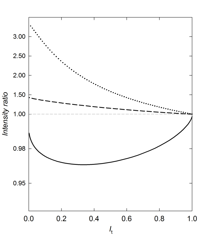
Figure 3: Ratio of approximate intensity and exact intensity of void component $\tau_{t}$ in dependence of the exact intensity $I_{t}$ according to eq. (31). Approximate intensity: entirely diffusion-limited trapping ($\cdot\cdot\cdot$) [Eq. (42)], entirely reaction-controlled trapping ($---$) [Eq. (39)], and simple trapping model [Eq. (39)] with effective diffusion-trapping rate $K_{eff}$ [Eq. (60)] (—). Note the different scales of the ratio axis for ratios $<1$ and $>1$. Parameters: $\Omega^{-1}=6\times 10^{28}$ m^-3, others as in Fig. 2.

The deviations of the two limiting cases from the exact solution become even more clear when the ratios of the trap component intensities of the limiting and exact solution is considered as shown in the upper part of Fig. 3. The deviation from the exact solution substantially increases with decreasing intensity, i.e., with decreasing void concentration. In this low concentration regime, the deviations attain a factor of ca. 1.5 (reaction limit) or larger than 3 (diffusion limit) for the present set of parameters, i.e., the entirely diffusion-limiting case deviates in this example more strongly than the reaction-limited case. Diffusion limitation gets even more pronounced when $e^{+}$ diffusivity is reduced, e.g., due to scattering at lattice imperfections. Regarding the opposite side of high defect concentrations, Fig. 3 (upper part) nicely demonstrates that deviations from the exact theory vanishes upon approaching $e^{+}$ saturation trapping since in this regime kinetic effects tends to become irrelevant.

IV.1.1 Comparison with effective rate approach

Next we compare the present model with approximations according to which diffusion limitation is taking account in the standard trapping model by means of a diffusion-limited trapping rate Frank and Seeger (1974); Bentzon and Evans (1990):

$$K_{diff}=\frac{4\pi r_{0}D}{\Omega}\times C_{t}\,.$$ (59)

The case of both transition- and diffusion-limited trapping, is treated in this approximation by means of the effective trapping rate Frank and Seeger (1974); Bentzon and Evans (1990)

$$K_{eff}=\frac{K_{diff}\sigma_{t}C_{t}}{K_{diff}+\sigma_{t}C_{t}}$$ (60)

with $\sigma_{t}$ and $C_{t}$ according to equations (1) and (7), respectively. We note that the diffusion-limited trapping rate according to eq. (59) is also included in the present model; in fact $K_{diff}$ is identical to the pre-factor of $I_{t}$ for entirely diffusion limited trapping [Eq. (42)] when the subtrahend $r_{0}^{3}$ in the nominator, which is associated with the defect volume, is omitted.

In figure 4 the concentration dependence of the relative intensity $I_{t}$ of the $e^{+}$ lifetime component $\tau_{t}$ in voids is shown for the exact models of diffusion-reaction [Eq. (31)] or entire diffusion limitation [Eq. (42)] in comparison with the corresponding approximations using the above mentioned effective or diffusion-trapping rates [Equations (59), (60)] with the simple trapping model [Eq. (39)]. Although the effective-rate approximations of the diffusion limitation describe the sigmoidal curve fairly well, deviations from the exact diffusion models are also apparent, e.g., for the example, $I_{t}=45$ %, mentioned above the deviation in concentration is ca. 7 % compared to the exact diffusion-reaction theory.

The deviations become clearer once more when we consider the intensity ratio of the effective-rate model and the exact theory, as plotted in the lower part of Fig. 3. Remarkably, since the effectice trapping rate $K_{eff}$ is lower than both the reaction-trapping rate $\sigma_{t}C_{t}$ and the diffusion-trapping rate $K_{diff}$, the intensity $I_{t}$ deduced from the effective trapping model is smaller than the exact value. Deviations from the full model occur throughout the entire intensity regime, although these deviations are less pronounced compared to the two limiting cases (fully reaction- or diffusion limited, upper part of Fig. 3). For applications in the analysis of experimental data, the accuracy of the effective rate approach [equation (60)] can be assessed by plotting the intensity ratio (lower part of Fig. 3) for the respective parameter set. Irrespectively whether deviations of the effective-rate approach are strong or minor only, the present model founded on diffusion-reaction theory is that which covers the underlying physics most accurately.

IV.1.2 Competitive trapping at point defects

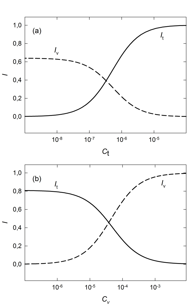
Figure 5: Relative intensities $I_{t}$ (—) [Eq. (45)] of void component $\tau_{t}$ and $I_{v}$ ($---$) [Eq. (46)] of vacancy component $\tau_{v}$ in dependence of (a) void concentration $C_{t}$ and (b) vacancy concentration $C_{v}$. Parameters: $\tau_{v}=250$ ps, $\sigma_{v}=4\times 10^{14}$ s^-1. $\Omega^{-1}=6\times 10^{28}$ m^-3, others as in Fig. 2. (a): $C_{v}=10^{-5}$ , (b) $C_{t}=10^{-6}$.

Now, we discuss the general case that in addition to diffusion-reaction controlled trapping at voids also competitive transition-limited trapping at vacancy-type defects in the lattice occurs (Sect. III.4). The relative intensities of the void component $I_{t}$ [Eq. (45)] and of the vacancy component $I_{v}$ [Eq. (46)] is plotted in figure 5 in dependence of void concentration $C_{t}$ (a) and vacancy concentration $C_{v}$ (b), for a given fixed $C_{v}$ or $C_{t}$, respectively. For the vacancy-type defect a $e^{+}$ lifetime component $\tau_{v}=250$ ps and a specific trapping rate $\sigma_{v}=4\times 10^{14}$ s^-1 Schaefer (1987) is assumed; the other parameters are the same as used above. The competitive $e^{+}$ trapping at voids and vacancy-type defects becomes evident. For a given vacancy concentration the intensity $I_{t}$ of the void increases and the intensity $I_{v}$ of the vacancy component decreases with increasing void concentration due to the increasing fraction of e⁺ that reaches the voids (Fig. 5.a). Likewise, for a given void concentration, $I_{v}$ increases and $I_{t}$ decreases with increasing vacancy concentration (Fig. 5.b).

IV.1.3 Comparison with $e^{+}$ trapping at grain boundaries

In the end of this subsection (IV.1), the results of the present model on diffusion-reaction limited $e^{+}$ trapping at extended spherical defects will briefly be compared with the corresponding model of $e^{+}$ trapping at grain boundaries of spherical crystallites with radius $R$ Würschum and Seeger (1996); Oberdorfer and Würschum (2009). Whereas in the latter case the surface of the diffusion sphere with area $4\pi R^{2}$ acts as $e^{+}$ trap, in the present case with voids of radius $r_{0}$, the trapping active area $4\pi r_{0}^{2}$ is much smaller. Moreover, the trapping rate $3\alpha/R$ for grain boundary trapping Oberdorfer and Würschum (2009) decreases much more slowly with increasing $R$ compared to the trapping rate $3\alpha r_{0}^{2}/(R^{3}-r_{0}^{3})$ of spherical extended defects with radius $r_{0}$ [Eq. 24]. This is the reason why diffusion limitation affects the kinetics of $e^{+}$ trapping at grain boundaries more strongly than in the case of voids which is nicely demonstrated in Fig. 6 where the exact solutions are compared with those of infinite diffusivities. In Fig. 6 the mean $e^{+}$ lifetime according to the exact solutions and those of the standard rate theory for the two types of extended traps are plotted. The exact solution for $e^{+}$ trapping at grain boundaries of spherical crystallites with radius $R$ reads Würschum and Seeger (1996); Oberdorfer and Würschum (2009)

$$\overline{\tau}=\tau_{f}+(\tau_{t}-\tau_{f})\times\frac{3\alpha L(\gamma_{0}R)}{R\gamma_{0}\Bigl{\{}\alpha+\gamma_{0}DL(\gamma_{0}R)\Bigl{\}}}\text{ with }L(z)=\coth z-\frac{1}{z}\,.$$ (61)

The more stronger deviation between the exact solution and the rate theory in the case of grain boundary trapping is obvious (Fig. 6).

IV.2 Larger precipitates: $e^{+}$-trapping from both sides of precipitate$-$matrix interface

In Sect. (III.5) we extended the model for applying it to larger precipitates taking into account free $e^{+}$ annihilation within the precipitate. The $e^{+}$ trapping from the precipitate into the precipitate$-$matrix interface is handled either by rate theory, for special cases where the precipitate radius is well below the $e^{+}$ diffusion length, or else by diffusion-reaction theory, for the more general case that the precipitate radius is in the range of or larger than the $e^{+}$ diffusion length. With this extension the present model is applicable to a wide variety of structurally complex scenarios, namely to all type of composite structures where spherical precipitates are embedded in a matrix irrespective of the size and the number density of the precipitates.

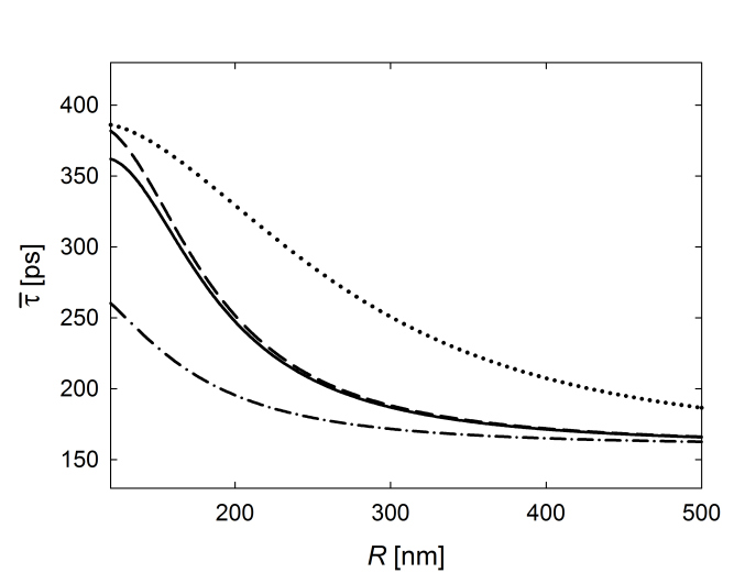
Figure 7: Mean $e^{+}$ lifetime in dependence of radius $R$ (i) for diffusion- and reaction limited $e^{+}$ trapping into the precipitate$-$matrix interface from both the matrix and the precipitate (—) [Eq. (III.5)], (ii) for diffusion- and reaction limited $e^{+}$ trapping from the matrix and entirely reaction-controlled trapping from the precipitate ($---$) [Eq. (III.5)], (iii) for entirely reaction-controlled trapping from both the matrix and the precipitate ($\cdot\cdot\cdot$) [Eq. (58)], and (iv) for rate-model as for (iii), but with effective diffusion-limited trapping rate [Eq. (60)] ($-\cdot-\cdot-$). Precipitate radius $r_{0}=100$ nm. Other parameters: $\tau_{f}=\tau_{c}=160$ ps, $\tau_{t}=400$ ps, $D=2\times 10^{-5}$ m²s^-1, $\alpha=\beta=3\times 10^{3}$ ms^-1. Note that $R$ is related to the precipitate concentration [Eq. 7].

Whereas for extended defects with smaller size, which were discussed in Sect. (IV.1), the deviations between the exact model and the rate theory may be of less relevance since the trapping active area $4\pi r_{0}^{2}$ is small, for larger precipitates the diffusion-limitation in any case gets relevant owing to the much larger trapping active area, similar as for $e^{+}$ trapping at GBs (see Fig. 6). This is demonstrated in Fig. 7, where the variation of the mean $e^{+}$ lifetime with radius $R$ is compared for four different solutions, namely diffusion-limitation of trapping into the precipitate$-$matrix interface from both the matrix and the precipitate, from the matrix only, and for entirely reaction-limited trapping from both sides with standard-trapping rate or with effective diffusion-limited trapping rate. The latter is obtained by replacing in equation (58) the standard-trapping rates by the effective diffusion-limited trapping rate according to equation (60), i.e., $3\alpha r_{0}^{2}(R^{3}-r_{0}^{3})^{-1}$ by $3\alpha Dr_{0}^{2}R^{-3}(\alpha r_{0}+D)^{-1}$ and $3\beta r_{0}^{-1}$ by $3\beta Dr_{0}^{-1}(\beta r_{0}+D)^{-1}$.

In contrast to the case of small extended defects (Fig. 6), for larger precipitates (example $r_{0}=100$ nm) substantial deviations between the solutions occur for the entire concentration regime if the diffusion-limitation is neglected (Fig. 7). Even the rate approach with effective diffusion-limited trapping rate, which at least for small extended defects is a reasonable approximation (Sect. IV.1.1, Fig. 4), turns out to be completely inadequate for the larger precipitate size. The deviations are much less if the diffusion-limitation is only neglected for the trapping from the precipitate into the interface, since the precipitate size (in contrast to the precipitate distance) remains in the range of the $e^{+}$ diffusion length independent of the precipitate concentration. Anyhow, for a precise description even for such small precipitate sizes, the exact theory of diffusion- and reaction controlled trapping has to be applied for the trapping from the interior of the precipitates.

Finally, we compare this model with that presented by Dryzek Dryzek (1999); Dryzek et al. (2016) for studying recrystallization in highly deformed metals. In that case recrystallized grains are embedded in a highly deformed matrix. Diffusion-limited $e^{+}$ trapping occurs from the grains into the matrix, whereas within the matrix saturation trapping of $e^{+}$ prevails due to the high defect density. In this sense, the model of Dryzek represents an extension of the diffusion-reaction theory for trapping at grain boundaries, where instead of GBs a surrounding deformed matrix is considered. The model presented here, represents a further extension where diffusion- and reaction-controlled trapping also from the matrix into the interfaces is considered.

V Conclusion

The present model with the exact solution of the diffusion-reaction theory for the $e^{+}$ trapping at extended spherical defects and competitive transition-limited trapping at atomic defects yields a basis for the quantitative description of the $e^{+}$ behaviour in materials with complex defect structure. It could be shown that the model includes as special cases the simple trapping model and the entirely diffusion-limited trapping, but both of these limiting cases represent approximations, only. For the full model, closed-form expressions were obtained for the mean positron lifetime $\overline{\tau}$ and for the intensities of the e⁺ lifetime components associated with trapping. This exact model allowed a quantitative assessment of the usual approach, which takes diffusion limitation for the trapping at voids into account by effective diffusion-trapping rates. The present closed-form solutions also renders this effective rate approach unnecessary.

The presented theory goes even much far beyond existing models, since it is not only applicable to small extended defects (such as voids or clusters), but also to larger precipitates where positron trapping from the precipitates into the precipitate$-$matrix interface is taken into consideration. Therefore, the model presents the basis for studying all type of composite structures where spherical precipitates are embedded in a matrix irrespective of their size and their number density.

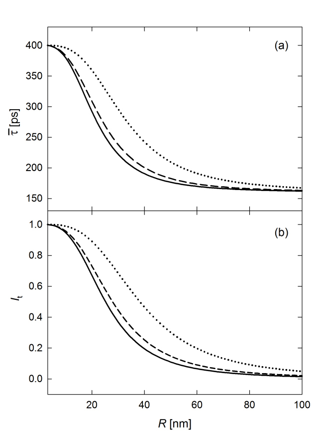
Figure 2: (a) Mean $e^{+}$ lifetime $\overline{\tau}$ and (b) relative intensity $I_{t}$ of void component $\tau_{t}$ in dependence of diffusion radius $R$ for diffusion-reaction model (—) [Equations (30), (31)], for standard rate ($---$) [Equations (38), (39)], and for limiting case of entirely diffusion-limited trapping ($\cdot\cdot\cdot$) [Equations (41), (42)]. Parameters: $\tau_{f}=160$ ps, $\tau_{t}=400$ ps, $D=2\times 10^{-5}$ m²s^-1, $\alpha=3\times 10^{3}$ ms^-1, $r_{0}=3$ nm. Note that $R$ is related to the void concentration [Eq. 7].

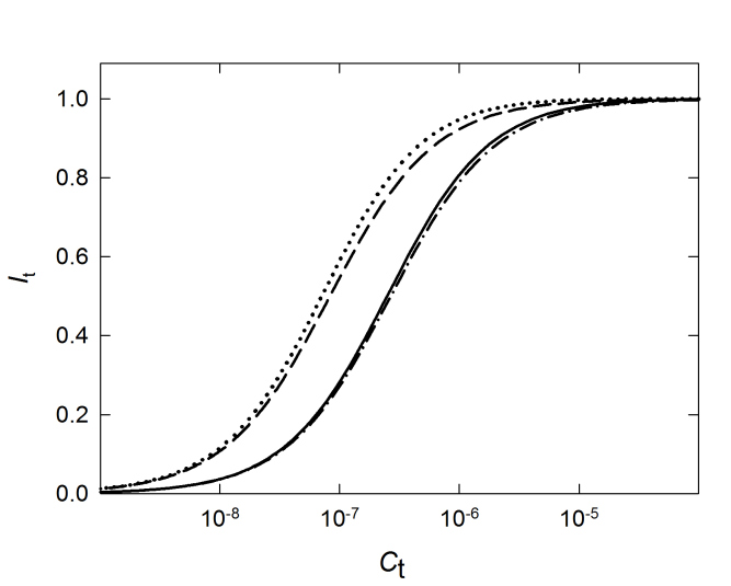
Figure 4: Relative intensity $I_{t}$ of void component $\tau_{t}$ in dependence of voids concentration $C_{t}$ for diffusion-reaction model (—) [Eq. (31)], for limiting case of entirely diffusion-limited trapping ($\cdot\cdot\cdot$) [Eq. (42)], as well as for simple trapping model [Eq. (39)] with effective trapping rate of diffusion $K_{diff}$ [Eq. (59)] ($---$) or with effective diffusion- and transition-limited trapping rate $K_{eff}$ [Eq. (60)] ($-\cdot-\cdot-$). Parameters: $\Omega^{-1}=6\times 10^{28}$ m^-3, others as in Fig. 2.

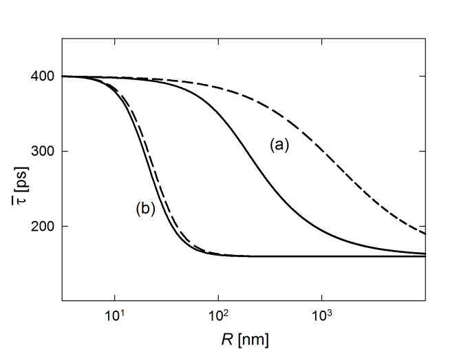
Figure 6: Comparison of mean $e^{+}$ lifetime $\overline{\tau}$ for diffusion-reaction limited $e^{+}$ trapping (a) at grain boundaries of spherical crystallites with radius $R$ Würschum and Seeger (1996); Oberdorfer and Würschum (2009) and (b) at extended spherical defects (present work, Fig. 2). (a) Exact solution according to eq. (61 Würschum and Seeger (1996) (—) and solution for standard rate theory ($---$) [Eq. 38] with trapping rate $K=3\alpha/R$; (b) exact solution [Eq. (30)] (—) and solution for standard rate theory ($---$) [Eq. (38)] with trapping rate $3\alpha r_{0}^{2}/(R^{3}-r_{0}^{3})$ [Eq. (24)]. Parameters as in Fig. 2.

[i] Intensities associated with positron annihilation from the free state
The sequence of intensities for poles $p=-\lambda_{0,j}$ given by Eq. (33) of [1] read:

$$I_{0,j}=\frac{K(\tau_{f}^{-1}-\tau_{t}^{-1})2(1+\gamma^{\star 2}_{j}R^{2})}{(\lambda_{0,j}-\tau_{f}^{-1})(\lambda_{0,j}-\tau_{t}^{-1})}\times$$ (62)

$$\Bigl{\{}\frac{D\gamma^{\star 2}_{j}}{\alpha r_{0}^{2}}\Bigl{[}R^{3}-r_{0}^{3}+(R-r_{0})r_{0}^{2}R^{2}(\gamma^{\star 2}_{j}+\frac{\alpha^{2}}{D^{2}})+\frac{\alpha r_{0}}{D}R^{2}(2R-r_{0})\Bigr{]}-1-\frac{\alpha r_{0}}{D}\Bigr{\}}^{-1}$$

with

$$\gamma^{\star 2}_{j}=\frac{\lambda_{0,j}-\tau_{f}^{-1}}{D}$$ (63)

and

$$K=\frac{3\alpha r_{0}^{2}}{R^{3}-r_{0}^{3}}\,.$$ (64)

As usual for this kind of diffusion-reaction problems, the intensities of these decay rates rapidly decrease (see eaxmple, Table I).
Limiting case of entirely reaction-controlled trapping
Expansion of $\tan(z)$ in Eq. (33) [1] up to third order yields for $D\rightarrow\infty$:

$$\lambda_{0}=\frac{1}{\tau_{0}}=\frac{1}{\tau_{f}}+K\,.$$ (65)

Inserting $\gamma^{\star 2}=K/D$ in Eq. (62) yields with $\lambda_{0}-\tau_{f}^{-1}=K$ for $D\rightarrow\infty$:

$$I_{0}\simeq\frac{K(\tau_{f}^{-1}-\tau_{t}^{-1})2}{(\lambda_{0}-\tau_{f}^{-1})(\lambda_{0}-\tau_{t}^{-1})\Bigl{\{}\frac{K}{\alpha r_{0}^{2}}(R^{3}-r_{0}^{3})-1\Bigr{\}}}=\frac{\tau_{f}^{-1}-\tau_{t}^{-1}}{\tau_{0}^{-1}-\tau_{f}^{-1}}\,.$$ (66)

The equations (65) and (66) correspond to the solutions of the standard two-state trapping theory, i.e., the present model includes in the limiting case of high positron diffusivity the solution of the standard-rate theory.
[ii] Inspection of pole $p=-1/\tau_{f}$
Expansion of $\tanh(z)$ up to third order yields for the second fraction $F$ of Eq. (29) [1]:

$$F=\frac{1/3\gamma^{3}(R^{3}-r_{0}^{3})}{1/3\gamma^{3}(R^{3}-r_{0}^{3})+\frac{\alpha r_{0}}{D}(\gamma r_{0}+1/3\gamma^{3}\hat{R}^{3})}=\frac{\gamma^{2}}{\gamma^{2}+\frac{K}{D}(1+\gamma^{2}\frac{\hat{R}^{3}}{3r_{0}})}$$ (67)

By means of eq. (67) $\tilde{n}(p)$ (Eq. (29) of [1]) can be written as:

$$\tilde{n}(p)=\frac{\tau_{t}^{-1}+p+K+\frac{K}{D}\frac{\hat{R}^{3}}{3r_{0}}(\tau_{t}^{-1}+p)}{(\tau_{t}^{-1}+p)\{\tau_{f}^{-1}+p+K[1+\frac{\hat{R}^{3}}{3Dr_{0}}(\tau_{f}^{-1}+p)]\}}$$ (68)

Limiting cases

• For the limiting case $p=-1/\tau_{f}$ eq. (68) reads:

  $$\tilde{n}(-\tau_{f}^{-1})=\frac{\tau_{t}^{-1}-\tau_{f}^{-1}+K+\frac{K}{D}\frac{\hat{R}^{3}}{3r_{0}}(\tau_{t}^{-1}-\tau_{f}^{-1})}{(\tau_{t}^{-1}-\tau_{f}^{-1})K}\,.$$ (69)

  Eq. (69) shows there is no singularity for $p=-1/\tau_{f}$. Since the residue of a removable singularity is zero, the positron lifetime spectrum does not contain a component $\tau_{f}$, as expected in the case of positron trapping.

• For the limiting case $D\rightarrow\infty$ eq. (68) reads:

  $$\tilde{n}(p)=\frac{\tau_{t}^{-1}+p+K}{(\tau_{t}^{-1}+p)(\tau_{f}^{-1}+p+K)}\,.$$ (70)

  Eq. (70) yields two poles which correspond to the two positron lifetime components $\tau_{t}$ and $1/(\tau_{f}^{-1}+K)$ according to the the standard two-state trapping model, i.e., the present model includes in the limiting case of high positron diffusivity the solution of the standard-rate theory.

Table 1: Sequence of first-order poles $p=-\lambda_{0,j}$ (eq. (33), [1]) and their corresponding intensities $I_{0,j}$ (eq. (62)), intensity $I_{t}$ (eq. (30), [1]) of the positron lifetime component $\tau_{t}$ and sum of all intensities $I_{total}$ for different values of $R$. Parameters (as for Fig. 2 of [1]): $\tau_{f}=160$ ps, $\tau_{t}=400$ ps, $D=2\times 10^{-5}$ m²s^-1, $\alpha=3\times 10^{3}$ ms^-1, $r_{0}=3$ nm.

$R=10$ nm	$j$	$\lambda_{0,j}$ [$s^{-1}$]	$I_{0,j}$ [%]	$I_{t}$ [%]	$I_{total}$ [%]
	1	7.375 $\times$ $10^{10}$	5.26	94.74	100.00
	2	5.581 $\times$ $10^{12}$	7.74 $\times$ $10^{-5}$
	3	1.805 $\times$ $10^{13}$	3.46 $\times$ $10^{-6}$

$R=25$ nm	$j$	$\lambda_{0,j}$ [$s^{-1}$]	$I_{0,j}$ [%]	$I_{t}$ [%]	$I_{total}$ [%]
	1	1.008 $\times$ $10^{10}$	49.44	50.56	100.00
	2	7.117 $\times$ $10^{11}$	1.91 $\times$ $10^{-4}$
	3	2.113 $\times$ $10^{12}$	1.68 $\times$ $10^{-5}$

$R=50$ nm	$j$	$\lambda_{0,j}$ [$s^{-1}$]	$I_{0,j}$ [%]	$I_{t}$ [%]	$I_{total}$ [%]
	1	6.712 $\times$ $10^{9}$	89.01	10.99	100.00
	2	1.745 $\times$ $10^{11}$	2.23 $\times$ $10^{-4}$
	3	5.037 $\times$ $10^{11}$	2.35 $\times$ $10^{-5}$

[1] R. Würschum, L. Resch, and G. Klinser, Phys. Rev. B 97 (2018) 224108.