A Bayesian Perspective on the Deep Image Prior

Abstract

The deep image prior [26] was recently introduced as a prior for natural images. It represents images as the output of a convolutional network with random inputs. For “inference”, gradient descent is performed to adjust network parameters to make the output match observations. This approach yields good performance on a range of image reconstruction tasks. We show that the deep image prior is asymptotically equivalent to a stationary Gaussian process prior in the limit as the number of channels in each layer of the network goes to infinity, and derive the corresponding kernel. This informs a Bayesian approach to inference. We show that by conducting posterior inference using stochastic gradient Langevin dynamics we avoid the need for early stopping, which is a drawback of the current approach, and improve results for denoising and impainting tasks. We illustrate these intuitions on a number of 1D and 2D signal reconstruction tasks.

1 Introduction

It is well known that deep convolutional networks trained on large datasets provide a rich hierarchical representation of images. Surprisingly, several works have shown that convolutional networks with random parameters can also encode non-trivial image properties. For example, second-order statistics of filter responses of random convolutional networks are effective for style transfer and synthesis tasks [27]. On small datasets, features extracted from random convolutional networks can work just as well as trained networks [24]. Along these lines, the “deep image prior” proposed by Ulyanov et al. [26] showed that the output of a suitably designed convolutional network on random inputs tends to be smooth and induces a natural image prior, so that the search over natural images can be replaced by gradient descent to find network parameters and inputs to minimize a reconstruction error of the network output. Remarkably, no prior training is needed and the method operates by initializing the parameters randomly.

Our work provides a novel Bayesian view of the deep image prior. We prove that a convolutional network with random parameters operating on a stationary input, e.g., white noise, approaches a two-dimensional Gaussian process (GP) with a stationary kernel in the limit as the number of channels in each layer goes to infinity (Theorem 1). While prior work [19, 31, 18, 3, 20] has investigated the GP behavior of infinitely wide networks and convolutional networks, our work is the first to analyze the spatial covariance structure induced by a convolutional network on stationary inputs. We analytically derive the kernel as a function of the network architecture and input distribution by characterizing the effects of convolutions, non-linearities, up-sampling, down-sampling, and skip connections on the spatial covariance. These insights could inform choices of network architecture for designing 1D or 2D priors.

We then use a Bayesian perspective to address drawbacks of current estimation techniques for the deep image prior. Estimating parameters in a deep network from a single image poses a huge risk of overfitting. In prior work the authors relied on early stopping to avoid this. Bayesian inference provides a principled way to avoid overfitting by adding suitable priors over the parameters and then using posterior distributions to quantify uncertainty. However, posterior inference with deep networks is challenging. One option is to compute the posterior of the limiting GP. For small networks with enough channels, we show this closely matches the deep image prior, but is computationally expensive. Instead, we conduct posterior sampling based on stochastic gradient Langevin dynamics (SGLD) [28], which is both theoretically well founded and computationally efficient, since it is based on standard gradient descent. We show that posterior sampling using SGLD avoids the need for early stopping and performs better than vanilla gradient descent on image denoising and inpainting tasks (see Figure 1). It also allows us to systematically compute variances of estimates as a measure of uncertainty. We illustrate these ideas on a number of 1D and 2D reconstruction tasks.

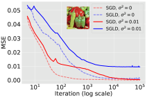
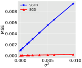
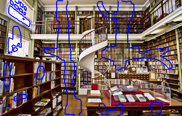
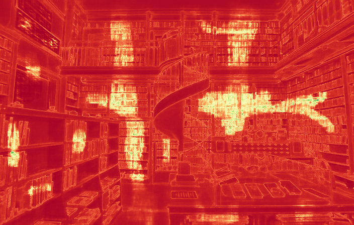
(a) MSE vs. Iteration	(b) Final MSE vs. $\sigma^{2}$	(c) Inferred mean	(d) Inferred variance

Figure 1: (Best viewed magnified.) Denoising and inpainiting results with the deep image prior. (a) Mean Squared Error (MSE) of the inferred image with respect to the noisy input image as a function of iteration for two different noise levels. SGD converges to zero MSE resulting in overfitting while SGLD roughly converges to the noise level in the image. This is also illustrated in panel (b) where we plot the MSE of SGD and SGLD as a function of the noise level $\sigma^{2}$ after convergence. See Section 5.2.1 for implementation details. (c) An inpainting result where parts of the image inside the blue boundaries are masked out and inferred using SGLD with the deep image prior. (d) An estimate of the variance obtained from posterior samples visualized as a heat map. Notice that the missing regions near the top left have lower variance as the area is uniform.

2 Related work

Image priors. Our work analyzes the deep image prior [26] that represents an image as a convolutional network $f$ with parameters $\theta$ on input $x$. Given a noisy target $y$ the denoised image is obtained by minimizing the reconstruction error $\|y-f(x;\theta)\|$ over $x$ and $\theta$. The approach starts from an initial value of $x$ and $\theta$ drawn i.i.d. from a zero mean Gaussian distribution and optimizes the objective through gradient descent, relying on early stopping to avoid overfitting (see Figure 1). Their approach showed that the prior is competitive with state-of-the-art learning-free approaches, such as BM3D [6], for image denoising, super resolution, and inpainting tasks. The prior encodes hierarchical self-similarities that dictionary-based approaches [21] and non-local techniques such as BM3D and non-local means [4] exploit. The architecture of the network plays a crucial role: several layer networks were used for inpainting tasks, while those with skip connections were used for denoising. Our work shows that these networks induce priors that correspond to different smoothing “scales”.

Gaussian processes (GPs). A Gaussian processes is an infinite collection of random variables for which any finite subset are jointly Gaussian distributed [23]. A GP is commonly viewed as a prior over functions. Let $T$ be an index set (e.g., $T=\mathbb{R}$ or $T=\mathbb{R}^{d}$) and let $\mu(t)$ be a real-valued mean function and $K(t,t^{\prime})$ be a non-negative definite kernel or covariance function on $T$. If $f\sim GP(\mu,K)$, then, for any finite number of indices $t_{1},\ldots,t_{n}\in T$, the vector $(f(t_{i}))_{i=1}^{n}$ is Gaussian distributed with mean vector $(\mu(t_{i}))_{i=1}^{n}$ and covariance matrix $(K(t_{i},t_{j}))_{i,j=1}^{n}$. GPs have a long history in spatial statistics and geostatistics [17]. In ML, interest in GPs was motivated by their connections to neural networks (see below). GPs can be used for general-purpose Bayesian regression [31, 22], classification [30], and many other applications [23].

Deep networks and GPs. Neal [19] showed that a two-layer network converges to a Gaussian process as its width goes to infinity. Williams [29] provided expressions for the covariance function of networks with sigmoid and Gaussian transfer functions. Cho and Saul [5] presented kernels for the ReLU and the Heaviside step non-linearities and investigated their effectiveness with kernel machines. Recently, several works [13, 18] have extended these results to deep networks and derived covariance functions for the resulting GPs. Similar analyses have also been applied to convolutional networks. Garriaga-Alonso et al. [9] investigated the GP behavior of convolutional networks with residual layers, while Borovykh [3] analyzed the covariance functions in the limit when the filter width goes to infinity. Novak et al. [20] evaluated the effect of pooling layers in the resulting GP. Much of this work has been applied to prediction tasks, where given a dataset ${\cal D}=\{(x_{i},y_{i})\}_{i=1}^{n}$, a covariance function induced by a deep network is used to estimate the posterior $p(y|x,{\cal D})$ using standard GP machinery. In contrast, we view a convolutional network as a spatial random process over the image coordinate space and study the induced covariance structure.

Bayesian inference with deep networks. It has long been recognized that Bayesian learning of neural networks weights would be desirable [15, 19], e.g., to prevent overfitting and quantify uncertainty. Indeed, this was a motivation in the original work connecting neural networks and GPs. Performing MAP estimation with respect to a prior on the weights is computationally straightforward and corresponds to regularization. However, the computational challenges of full posterior inference are significant. Early works used MCMC [19] or the Laplace approximation [7, 15] but were much slower than basic learning by backpropagation. Several variational inference (VI) approaches have been proposed over the years [12, 1, 10, 2]. Recently, dropout was shown to be a form of approximate Bayesian inference [8]. The approach we will use is based on stochastic gradient Langevin dynamics (SGLD) [28], a general-purpose method to convert SGD into an MCMC sampler by adding noise to the iterates. Li et al. [14] describe a preconditioned SGLD method for deep networks.

3 Limiting GP for Convolutional Networks

Previous work focused on the covariance of (scalar-valued) network outputs for two different inputs (i.e., images). For the deep image prior, we are interested in the spatial covariance structure within each layer of a convolutional network. As a basic building block, we consider a multi-channel input image $X$ transformed through a convolutional layer, an elementwise non-linearity, and then a second convolution to yield a new multi-channel “image” $Z$, and derive the limiting distribution of a representative channel $z$ as the number of input channels and filters go to infinity. First, we derive the limiting distribution when $X$ is fixed, which mimics derivations from previous work. We then let $X$ be a stationary random process, and show how the spatial covariance structure propagates to $z$, which is our main result. We then apply this argument inductively to analyze multi-layer networks, and also analyze other network operations such as upsampling, downsampling, etc.

3.1 Limiting Distribution for Fixed $X$

For simplicity, consider an image $X\in\mathbb{R}^{c\times T}$ with $c$ channels and only one spatial dimension. The derivations are essentially identical for two or more spatial dimensions. The first layer of the network has $H$ filters denoted by $U=(u_{1},u_{2},\ldots u_{H})$ where $u_{k}\in\mathbb{R}^{c\times d}$ and the second layer has one filter $v\in\mathbb{R}^{H}$ (corresponding to a single channel of the output of this layer). The output of this network is:

$$z=v*h(X*U)=\sum_{k=1}^{H}v_{k}h(X*u_{k}).$$

The output $z=(z(1),z(2),\ldots,z(T^{\prime}))$ also has one spatial dimension. Following [19, 29] we derive the distribution of $z$ when $U\sim N(0,\sigma_{u}^{2}\mathbb{I})$ and $v\sim N(0,\sigma_{v}^{2}\mathbb{I})$. The mean is

$$\begin{split}\mathbb{E}[z(t)]&=\mathbb{E}\left[\sum_{k=1}^{H}v_{k}h\left((X*u_{k})(t)\right)\right]\\ &=\mathbb{E}\left[\sum_{k=1}^{H}v_{k}h\left(\sum_{i=1,j=1}^{c,d}x(i,t+1-j){u}_{k}(i,j)\right)\right].\end{split}$$

By linearity of expectation and independence of $u$ and $v$,

$$\mathbb{E}[z(t)]=\sum_{k=1}^{H}\mathbb{E}[v_{k}]\mathbb{E}\left[h\left((X*u_{k})(t)\right)\right]=0,$$

since $v$ has a mean of zero. The central limit theorem (CLT) can be applied when $h$ is bounded to show that $z(t)$ approaches in distribution to a Gaussian as $H\rightarrow\infty$ and $\sigma^{2}_{v}$ is scaled as $1/H$. Note that $u$ and $v$ don’t need to be Gaussian for the CLT to apply, but we will use this property to derive the covariance. This is given by

$$\begin{split}K_{z}(t_{1},t_{2})={}&\mathbb{E}[z(t_{1})z(t_{2})]\\ ={}&\mathbb{E}\left[\sum_{k=1}^{H}v_{k}^{2}h\big{(}(X*u_{k})(t_{1})\big{)}h\big{(}(X*u_{k})(t_{2})\big{)}\right]\\ ={}&H\sigma_{v}^{2}\mathbb{E}\left[h\big{(}(X*u_{1})(t_{1})\big{)}h\big{(}(X*u_{1})(t_{2})\big{)}\right].\end{split}$$

The last two steps follow from the independence of $u$ and $v$ and that $v$ is drawn from a zero mean Gaussian. Let $\bar{x}(t)={\rm vec}\left([X(:,t),X(:,t-1),\ldots,X(:,t-d+1)]\right)$ be the flattened tensor with elements within the window of size $d$ at position $t$ of $X$. Similarly denote $\bar{u}={\rm vec}(u)$. Then the expectation can be written as

$$K_{z}(t_{1},t_{2})=H\sigma_{v}^{2}E_{u}\left[h(\bar{x}(t_{1})^{T}\bar{u})h(\bar{x}(t_{2})^{T}\bar{u})\right].$$ (1)

Williams [29] showed $V(x,y)=E_{u}\left[h(x^{T}u)h(y^{T}u)\right]$ can be computed analytically for various transfer functions. For example, when $h(x)={\rm erf}(x)=2/\sqrt{\pi}\int_{0}^{x}e^{-s^{2}}ds$, then

$$V_{{\rm erf}}(x,y)=\frac{2}{\pi}\sin^{-1}\frac{x^{T}\Sigma y}{\sqrt{\left(x^{T}\Sigma x\right)\left(y^{T}\Sigma y\right)}}.$$ (2)

Here $\Sigma=\sigma^{2}\mathbb{I}$ is the covariance of $u$. Williams also derived kernels for the Gaussian transfer function $h(x,u)=\exp\{-(x-u)^{T}(x-u)/2\sigma^{2}\}$. For the ReLU non-linearity, i.e., $h(t)=\max(0,t)$, Cho and Saul [5] derived the expectation as:

$$V_{\rm relu}(x,y)=\frac{1}{2\pi}\|x\|\|y\|\big{(}\sin\theta+(\pi-\theta)\cos\theta\big{)},$$ (3)

where $\theta=\cos^{-1}\left(\frac{x^{T}y}{\|x\|\|y\|}\right)$. We refer the reader to [5, 29] for expressions corresponding to other transfer functions.

Thus, letting $\sigma_{v}^{2}$ scale as $1/H$ and $H\rightarrow\infty$ and for any input $X$, the output $z$ of our basic convolution-nonlinearity-convolution building block converges to a Gaussian distribution with zero mean and covariance

$$K_{z}(t_{1},t_{2})=V\left(\bar{x}(t_{1}),\bar{x}(t_{2})\right).$$ (4)

3.2 Limiting Distribution for Stationary $X$

We now consider the case when channels of $X$ are drawn i.i.d. from a stationary distribution. A signal $x$ is stationary (in the weak- or wide-sense) if the mean is position invariant and the covariance is shift invariant, i.e.,

$$m_{x}=\mathbb{E}[x(t)]=\mathbb{E}[x(t+\tau)],~{}~{}\forall\tau$$ (5)

and

$$\begin{split}K_{x}(t_{1},t_{2})&=\mathbb{E}[(x(t_{1})-m_{x})(x(t_{2})-m_{x})]\\ &=K_{x}(t_{1}-t_{2}),\forall t_{1},t_{2}.\end{split}$$ (6)

An example of a stationary distribution is white noise where $x(i)$ is i.i.d. from a zero mean Gaussian distribution $N(0,\sigma^{2})$ resulting in a mean $m_{x}=0$ and covariance $K_{x}(t_{1},t_{2})=\sigma^{2}\mathbf{1}[t_{1}=t_{2}]$. Note that the input for the deep image prior is drawn from this distribution.

Theorem 1.

Let each channel of $X$ be drawn independently from a zero mean stationary distribution with covariance function $K_{x}$. Then the output of a two-layer convolutional network with the sigmoid non-linearity, i.e., $h(t)={\rm erf}(t)$, converges to a zero mean stationary Gaussian process as the number of input channels $c$ and filters $H$ go to infinity sequentially. The stationary covariance $K_{z}$ is given by

$$K_{z}^{\rm erf}(t_{1},t_{2})=K_{z}(r)=\frac{2}{\pi}\sin^{-1}\frac{K_{x}(r)}{K_{x}(0)}.$$

where $r=t_{2}-t_{1}$.

The full proof is included in the Appendix and is obtained by applying the continious mapping thorem [16] on the formula for the sigmoid non-linearity. The theorem implies that the limiting distribution of $Z$ is a stationary GP if the input $X$ is stationary.

Lemma 1.

Assume the same conditions as Theorem 1 except the non-linearity is replaced by ReLU. Then the output converges to a zero mean stationary Gaussian process with covariance $K_{z}$

$$K_{z}^{\rm relu}(t_{1},t_{2})=\frac{K_{x}(0)}{2\pi}\Big{(}\sin\theta^{x}_{t_{1},t_{2}}+(\pi-\theta^{x}_{t_{1},t_{2}})\cos\theta^{x}_{t_{1},t_{2}}\Big{)},$$ (7)

where $\theta^{x}_{t_{1},t_{2}}=\cos^{-1}\left(K_{x}(t_{1},t_{2})/K_{x}(0)\right)$. In terms of the angles we get the following:

$$\cos\theta^{z}_{t_{1},t_{2}}=\frac{1}{\pi}\Big{(}\sin\theta^{x}_{t_{1},t_{2}}+(\pi-\theta^{x}_{t_{1},t_{2}})\cos\theta^{x}_{t_{1},t_{2}}\Big{)}.$$

This can be proved by applying the recursive formula for ReLU non-linearity [5]. One interesting observation is that, for both non-linearities, the output covariance $K_{z}(r)$ at a given offset $r$ only depends on the input covariance $K_{x}(r)$ at the same offset, and on $K_{x}(0)$.

Two or more dimensions. The results of this section hold without modification and essentially the same proofs for inputs with $c$ channels and two or more spatial dimensions by letting $t_{1}$, $t_{2}$, and $r=t_{2}-t_{1}$ be vectors of indices.

3.3 Beyond Two Layers

So far we have shown that the output of our basic two-layer building block converges to a zero mean stationary Gaussian process as $c\to\infty$ and then $H\to\infty$. Below we discuss the effect of adding more layers to the network.

Convolutional layers. A proof of GP convergence for deep networks was presented in [18], including the case for transfer functions that can be bounded by a linear envelope, such as ReLU. In the convolutional setting, this implies that the output converges to GP as the number of filters in each layer simultaneously goes to infinity. The covariance function can be obtained by recursively applying Theorem 1 and Lemma 1; stationarity is preserved at each layer.

Bias term. Our analysis holds when a bias term $b$ sampled from a zero-mean Gaussian is added, i.e., $z^{\rm bias}=z+b$. In this case the GP is still zero-mean but the covariance function becomes: $K^{\rm bias}_{z}(t_{1},t_{2})=\sigma_{b}^{2}+K_{z}(t_{1},t_{2})$, which is still stationary.

Upsampling and downsampling layers. Convolutional networks have upsampling and downsampling layers to induce hierarchical representations. It is easy to see that downsampling (decimating) the signal preserves stationarity since $K^{\downarrow}_{x}(t_{1},t_{2})=K_{x}(\tau t_{1},\tau t_{2})$ where $\tau$ is the downsampling factor. Downsampling by average pooling also preserves stationarity. The resulting kernel can be obtained by applying a uniform filter corresponding to the size of the pooling window, which results in a stationary signal, followed by downsampling. However, upsampling in general does not preserve stationarity. Therrien [25] describes the conditions under which upsampling a signal with a linear filter maintains stationarity. In particular, the upsampling filter must be band limited, such as the ${\rm sinc}$ filter: ${\rm sinc}(x)=\sin(x)/x$. If stationarity is preserved the covariance in the next layer is given by $K^{\uparrow}_{x}(t_{1},t_{2})=K_{x}(t_{1}/\tau,t_{2}/\tau)$.

Skip connections. Modern convolutional networks have skip connections where outputs from two layers are added $Z=X+Y$ or concatenated $Z=[X;Y]$. In both cases if $X$ and $Y$ are stationary GPs so is $Z$. See [9] for a discussion.

4 Bayesian Inference for Deep Image Prior

Let’s revisit the deep image prior for a denoising task. Given an noisy image $\hat{y}$ the deep image prior solves

$$\min_{\theta,x}||\hat{y}-f(x,\theta)||_{2}^{2},$$

where $x$ is the input and $\theta$ are the parameters of an appropriately chosen convolutional network. Both $x$ and $\theta$ are initialized randomly from a prior distribution. Optimization is performed using stochastic gradient descent (SGD) over $x$ and $\theta$ (optionally $x$ is kept fixed) and relying on early stopping to avoid overfitting (see Figures 1 and 2). The denoised image is obtained as $y^{*}=f(x^{*},\theta^{*})$.

The inference procedure can be interpreted as a maximum likelihood estimate (MLE) under a Gaussian noise model: $\hat{y}=y+\epsilon$, where $\epsilon=N(0,\sigma_{n}^{2}\mathbb{I})$. Bayesian inference suggests we add a suitable prior $p(x,\theta)$ over the parameters and reconstruct the image by integrating the posterior, to get $y^{*}=\int p(x,\theta\mid\hat{y})f(x,\theta)dxd\theta,$ The obvious computational challenge is computing this posterior average. An intermediate option is maximum a posteriori (MAP) inference where the argmax of the posterior is used. However both MLE and MAP do not capture parameter uncertainty and can overfit to the data.

In standard MCMC the integral is replaced by a sample average of a Markov chain that converges to the true posterior. However convergence with MCMC techniques is generally slower than backpropagation for deep networks. Stochastic gradient Langevin dyanamics (SGLD) [28] provides a general framework to derive an MCMC sampler from SGD by injecting Gaussian noise to the gradient updates. Let $w=(x,\theta)$. The SGLD update is:

$$\begin{split}\Delta_{w}&=\frac{\epsilon}{2}\Big{(}\nabla_{w}\log p(\hat{y}\mid w)+\nabla_{w}\log p(w)\Big{)}+\eta_{t}\\ \eta_{t}&\sim N(0,\epsilon).\end{split}$$ (8)

where $\epsilon$ is the step size. Under suitable conditions, e.g., $\sum\epsilon_{t}=\infty$ and $\sum\epsilon_{t}^{2}<\infty$ and others, it can be shown that $w_{1},w_{2},\ldots$ converges to the posterior distribution. The log-prior term is implemented as weight decay.

Our strategy for posterior inference with the deep image prior thus adds Gaussian noise to the gradients at each step to estimate the posterior sample averages after a “burn in” phase. As seen in Figure 1(a), due to the Gaussian noise in the gradients, the MSE with respect to the noisy image does not go to zero, and converges to a value that is close to the noise level as seen in Figure 1(b). It is also important to note that MAP inference alone doesn’t avoid overfitting. Figure 2 shows a version where weight decay is used to regularize parameters, which also overfits to the noise. Further experiments with inference procedures for denoising are described in Section 5.2.

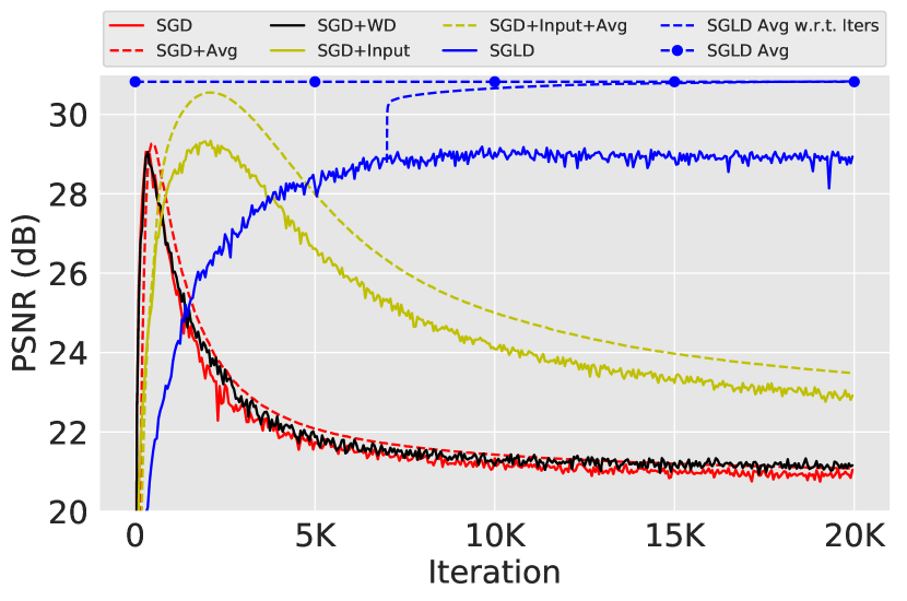
Figure 2: The PSNR curve for different learning methods on the “peppers” image of Figure 1. The SGD and its variants use early stopping to avoid overfitting. MAP inference by adding a prior term (WD: weight decay) shown as the black curve doesn’t avoid overfitting. Moving averages (dashed lines) and adding noise to the input improves performance. By contrast, samples from SGLD after “burn-in” remains stable and the posterior mean improves over the highest PSNR of the other approaches.

5 Experiments

5.1 Toy examples

We first study the effect of the architecture and input distribution on the covariance function of the stationary GP using 1D convolutional networks. We consider two architectures: (1) AutoEncoder: where $d$ conv + downsampling blocks are followed by $d$ conv + upsampling blocks, and (2) Conv: where convolutional blocks without any upsampling or downsampling. We use ReLU non-linearity after each conv layer in both cases. We also vary the input covariance $K_{x}$. Each channel of $X$ is first sampled iid from a zero-mean Gaussian with a variance $\sigma^{2}$. A simple way to obtain inputs with a spatial covariance $K_{x}$ equal to a Gaussian with standard deviation $\sigma$ is to then spatially filter channels of $X$ with a Gaussian filter with standard deviation $\sqrt{2}\sigma$.

Figure 3 shows the covariance function $\cos\theta_{t_{1},t_{2}}=K_{z}(t_{1}-t_{2})/K_{z}(0),$ induced by varying the $\sigma$ and depth $d$ of the two architectures (Figure 3a-b). We empirically estimated the covariance function by sampling many networks and inputs from the prior distribution. The covariance function for the convolutional-only architecture is also calculated using the recursion in Equation 7. For both architectures increasing $\sigma$ and $d$ introduce longer-range spatial covariances. For the auto-encoder upsampling induces longer-range interactions even when $\sigma$ is zero shedding some light on the role of upsampling in the deep image prior. Our network architectures have 128 filters, even so, the match between the empirical covariance and the analytic one is quite good as seen in Figure 3(b).

Figure 3(c) shows samples drawn from the prior of the convolutional-only architecture. Figure 3(d) shows the posterior mean and variance with SGLD inference where we randomly dropped 90% of the data from a 1D signal. Changing the covariance influences the mean and variance which is qualitatively similar to choosing the scale of stationary kernel in the GP: larger scales (bigger input $\sigma$ or depth) lead to smoother interpolations.

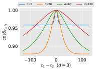
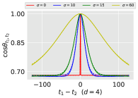
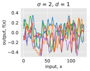
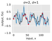
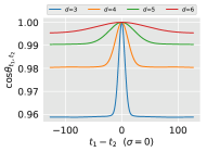
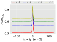
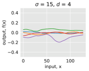
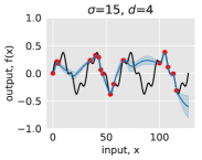
(a) $\cos\theta_{t_{1},t_{2}}$ (AE)	(b) $\cos\theta_{t_{1},t_{2}}$ (Conv)	(c) Prior	(d) Posterior

Figure 3: Priors and posterior with 1D convolutional networks. The covariance function $\cos\theta_{t_{1},t_{2}}=K(t_{1}-t_{2})/K(0)$ for the (a) AutoEncoder and (b) Conv architectures estimated empirically for different values of depth and input covariance. For the Conv architecture we also compute the covariance function analytically using recursion in Equation 7 shown as dashed lines in panel (b). The empirical estimates were obtained with networks with $256$ filters. The agreement is quite good for small values of sigma. For larger offsets the convergence towards a Gaussian is approximate. Panel (c) shows samples from the prior of the Conv architecture with two different configurations, and panel (d) shows the posterior means and variances estimated using SGLD.

5.2 Natural images

Throughout our experiments we adopt the network architecture reported in [26] for image denoising and inpainting tasks for a direct comparison with their results. These architectures are 5-layer auto-encoders with skip-connections and each layer contains 128 channels. We consider images from the standard image reconstruction datasets [6, 11]. For inference we use a learning rate of $0.01$ for image denoising and $0.001$ for image inpainting. We compare the following inference schemes:

1. SGD+Early: Vanilla SGD with early stopping.

2. SGD+Early+Avg: Averaging the predictions with exponential sliding window of the vanilla SGD.

3. SGD+Input+Early: Perturbing the input $x$ with an additive Gaussian noise with mean zero and standard deviation $\sigma_{p}$ at each learning step of SGD.

4. SGD+Input+Early+Avg: Averaging the predictions of the earlier approach with a exponential window.

5. SGLD: Averaging after burn-in iterations of posterior samples with SGLD inference.

We manually set the stopping iteration in the first four schemes to one with essentially the best reconstruction error — note that this is an oracle scheme and cannot be implemented in real reconstruction settings. For image denoising task, the stopping iteration is set as 500 for the first two schemes, and 1800 for the third and fourth methods. For image inpainting task, this parameter is set as 5000 and 11000 respectively.

The third and fourth variants were described in the supplementary material of [26] and in the released codebase. We found that injecting noise to the input during inference consistently improves results. However, as observed in [26], regardless of the noise variance $\sigma_{p}$, the network is able to drive the objective to zero, i.e., it overfits to the noise. This is also illustrated in Figure 1 (a-b).

Since the input $x$ can be considered as part of the parameters, adding noise to the input during inference can be thought of as approximate SGLD. It is also not beneficial to optimize $x$ in the objective and is kept constant (though adding noise still helps). SGLD inference includes adding noise to all parameters, $x$ and $\theta$, sampled from a Gaussian distribution with variance scaled as the learning rate $\eta$, as described in Equation 4. We used 7K burn-in iterations and 20K training iterations for image denoising task, 20K and 30K for image inpainting tasks. Running SGLD longer doesn’t improve results further. The weight-decay hyper-parameter for SGLD is set inversely proportional to the number of pixels in the image and equal to 5e-8 for a 1024$\times$1024 image. For the baseline methods, we did not use weight decay, which, as seen in Figure 2, doesn’t influence results for SGD.

5.2.1 Image denoising

We first consider the image denoising task using various inference schemes. Each method is evaluated on a standard dataset for image denoising [6], which consists of 9 colored images corrupted with noise of $\sigma=25$ .

Figure 2 presents the peak signal-to-noise ratio (PSNR) values with respect to the clean image over the optimization iterations. This experiment is on the “peppers” image from the dataset as seen in Figure 1. The performance of SGD variants (red, black and yellow curves) reaches a peak but gradually degrades. By contrast, samples using SGLD (blue curves) are stable with respect to PSNR, alleviating the need for early stopping. SGD variants benefit from exponential window averaging (dashed red and yellow lines), which also eventually overfits. Taking the posterior mean after burn in with SGLD (dashed blue line) consistently achieves better performance. The posterior mean at 20K iteration (dashed blue line with markers) achieves the best performance among the various inference methods.

Figure 7 shows a qualitative comparison of SGD with early stopping to the posterior mean of SGLD, which contains fewer artifacts. More examples are available in the Appendix. Table 1 shows the quantitative comparisons between the SGLD and the baselines. We run each method 10 times and report the mean and standard deviations. SGD consistently benefits from perturbing the input signal with noise-based regularization, and from moving averaging. However, as noted, these methods still have to rely on early stopping, which is hard to set in practice. By contrast, SGLD outperforms the baseline methods across all images. Our reported numbers (SGD + Input + Early + Avg) are similar to the single-run results reported in prior work (30.44 PSNR compared to ours of 30.33$\pm$0.03 PSNR.) SGLD improves the average PNSR to 30.81. As a reference, BM3D [6] obtains an average PSNR of 31.68.

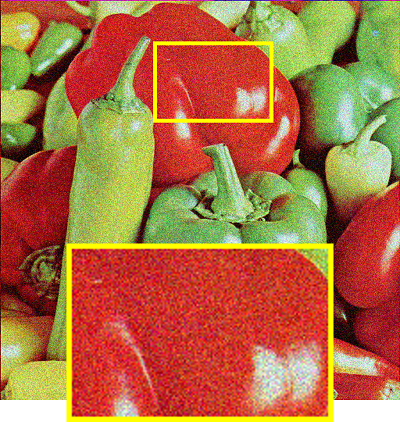
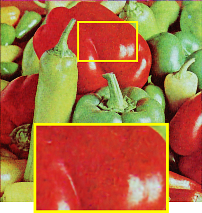
Input	SGD (28.38)	SGLD (30.82)

Figure 4: Image denoising results. Denoising the input noisy image with SGD and SGLD inference.

5.2.2 Image inpainting

For image inpainting we experiment on the same task as [26] where 50% of the pixels are randomly dropped. We evaluate various inference schemes on the standard image inpainting dataset [11] consisting of 11 grayscale images.

(a) Corrupted GT	(b) SGD	(c) +Avg.	(d) +Input	(e) +Input+Avg	(f) SGLD	(g) Uncertainty
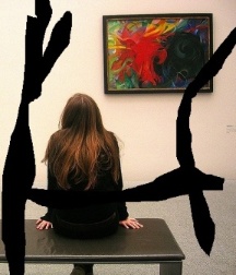
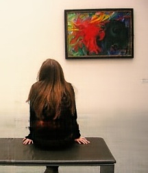
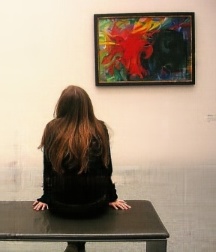
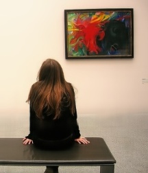
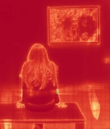
	27.86	28.06	28.51	28.53	31.43
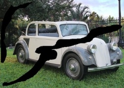
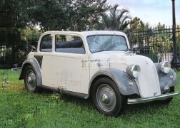
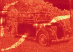
	22.85	22.97	23.31	23.57	27.10
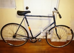
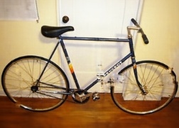
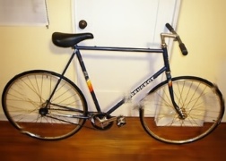
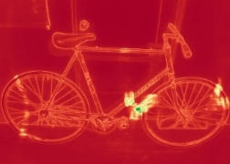
	25.35	26.52	26.48	26.74	28.87
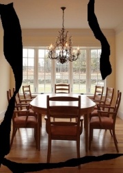
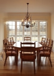
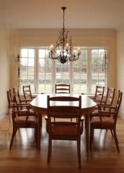
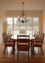
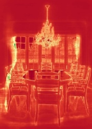
	28.16	28.18	28.71	29.04	30.78
	26.22	26.29	26.47	26.66	29.05
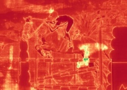
	26.04	26.09	26.11	26.28	28.41
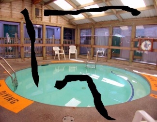
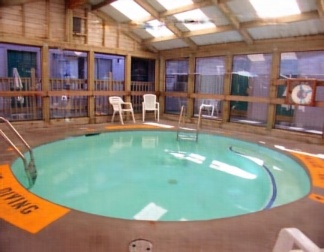
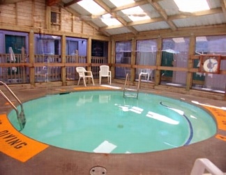
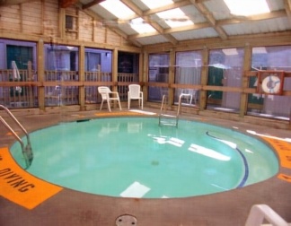
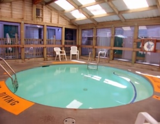
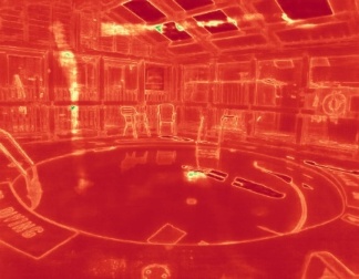
	29.03	29.15	30.15	30.33	32.95

Figure 8: (Best viewed magnified.) Comparison of inference schemes for image inpainting. (a) The input image with parts masked out. (b-f) Results using various inference schemes (see the previous figure and the main text for details of the methods). (f) SGLD achieves higher PSNR (shown underneath each figure) than the baseline methods (b-e). The early stopping iteration is set as 2000 for the first two schemes (b, c) and 3000 for the third and fourth methods (d, e). For these experiments we use a 6-layer auto-encoder without skip connections and random noise as input as reported in [26]. (g) The variance estimated from the posterior samples visualized as a heat map. Notice that the uncertainty is low in the missing regions that are surrounded by areas of relatively uniform appearance such as wall, sky and swimming pool, and higher in non-uniform areas such as those near the boundaries of different object in the image.

Table 2 presents a comparison between SGLD and the baseline methods. Similar to the image denoising task, the performance of SGD is improved by perturbing the input signal and additionally by averaging the intermediate samples during optimization. SGLD inference provides additional improvements; it outperforms the baselines and improves over the results reported in [26] from 33.48 to 34.51 PSNR. Figure 8 shows qualitative comparisons between SGLD and SGD. The posterior mean of SGLD has fewer artifacts than the best result generated by SGD variants.

Besides gains in performance, SGLD provides estimates of uncertainty. This is visualized in Figure 1(d). Observe that uncertainty is low in missing regions that are surrounded by areas of relatively uniform appearance such as the window and floor, and higher in non-uniform areas such as those near the boundaries of different object in the image.

Table 1: Image denoising task. Comparison of various inference schemes with the deep image prior for image denoising ($\sigma$=25). Bayesian inference with SGLD avoids the need for early stopping while consistently improves results. Details are described in Section 5.2.1.

	House	Peppers	Lena	Baboon	F16	Kodak1	Kodak2	Kodak3	Kodak12	Average
SGD + Early	26.74	28.42	29.17	23.50	29.76	26.61	28.68	30.07	29.78	28.08
	$\pm$0.41	$\pm$0.22	$\pm$0.25	$\pm$0.27	$\pm$0.49	$\pm$0.19	$\pm$0.18	$\pm$0.33	$\pm$0.17	$\pm$0.09
SGD + Early + Avg	28.78	29.20	30.26	23.82	31.17	27.14	29.88	31.00	30.64	29.10
	$\pm$0.35	$\pm$0.08	$\pm$0.12	$\pm$0.11	$\pm$0.1	$\pm$0.07	$\pm$0.12	$\pm$0.11	$\pm$0.12	$\pm$0.05
SGD + Input + Early	28.18	29.21	30.17	22.65	30.57	26.22	30.29	31.31	30.66	28.81
	$\pm$0.32	$\pm$0.11	$\pm$0.07	$\pm$0.08	$\pm$0.09	$\pm$0.14	$\pm$0.13	$\pm$0.08	$\pm$0.12	$\pm$0.04
SGD + Input + Early + Avg	30.61	30.46	31.81	23.69	32.66	27.32	31.70	32.86	31.87	30.33
	$\pm$0.3	$\pm$0.03	$\pm$0.03	$\pm$0.09	$\pm$0.06	$\pm$0.06	$\pm$0.03	$\pm$0.08	$\pm$0.1	$\pm$0.03
SGLD	30.86	30.82	32.05	24.54	32.90	27.96	32.05	33.29	32.79	30.81
	$\pm$0.61	$\pm$0.01	$\pm$0.03	$\pm$0.04	$\pm$0.08	$\pm$0.06	$\pm$0.05	$\pm$0.17	$\pm$0.06	$\pm$0.08
CMB3D [6]	33.03	31.20	32.27	25.95	32.78	29.13	32.44	34.54	33.76	31.68

Table 2: Image inpainting task. Comparison of various inference schemes with the deep image prior for image inpainting. SGLD estimates are more accurate while also providing a sensible estimate of the variance. Details are described in Section 5.2.2.

Method	Barbara	Boat	House	Lena	Peppers	C.man	Couple	Finger	Hill	Man	Montage	Average
SGD + Early	28.48	31.54	35.34	35.00	30.40	27.05	30.55	32.24	31.37	31.32	30.21	31.23
	$\pm$0.99	$\pm$0.23	$\pm$0.45	$\pm$0.25	$\pm$0.59	$\pm$0.35	$\pm$0.19	$\pm$0.16	$\pm$0.35	$\pm$0.29	$\pm$0.82	$\pm$0.11
SGD + Early + Avg	28.71	31.64	35.45	35.15	30.48	27.12	30.63	32.39	31.44	31.50	30.25	31.34
	$\pm$0.7	$\pm$0.28	$\pm$0.46	$\pm$0.18	$\pm$0.6	$\pm$0.39	$\pm$0.18	$\pm$0.12	$\pm$0.31	$\pm$0.39	$\pm$0.82	$\pm$0.08
SGD + Input + Early	32.48	32.71	36.16	36.91	33.22	29.66	32.40	32.79	33.27	32.59	33.15	33.21
	$\pm$0.48	$\pm$1.12	$\pm$2.14	$\pm$0.19	$\pm$0.24	$\pm$0.25	$\pm$2.07	$\pm$0.94	$\pm$0.07	$\pm$0.14	$\pm$0.46	$\pm$0.36
SGD + Input + Early + Avg	33.18	33.61	37.00	37.39	33.53	29.96	33.30	33.17	33.58	32.95	33.80	33.77
	$\pm$0.45	$\pm$0.3	$\pm$2.01	$\pm$0.14	$\pm$0.31	$\pm$0.3	$\pm$0.15	$\pm$0.77	$\pm$0.19	$\pm$0.16	$\pm$0.6	$\pm$0.23
SGLD	33.82	34.26	40.13	37.73	33.97	30.33	33.72	33.41	34.03	33.54	34.65	34.51
	$\pm$0.19	$\pm$0.12	$\pm$0.16	$\pm$0.05	$\pm$0.15	$\pm$0.15	$\pm$0.1	$\pm$0.04	$\pm$0.03	$\pm$0.06	$\pm$0.72	$\pm$0.08
Ulyanov et al. [26]	32.22	33.06	39.16	36.16	33.05	29.80	32.52	32.84	32.77	32.2	34.54	33.48
Papyan et al. [21]	28.44	31.44	34.58	35.04	31.11	27.90	31.18	31.34	32.35	31.92	28.05	31.19

5.3 Equivalence between GP and DIP

We compare the deep image prior (DIP) and its Gaussian process (GP) counterpart, both as prior and for posterior inference, and as a function of the number of filters in the network. For efficiency we used a U-Net architecture with two downsampling and upsampling layers for the DIP.

(a) DIP prior samples	(b) GP prior samples

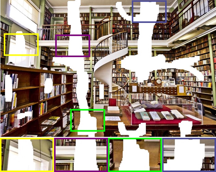
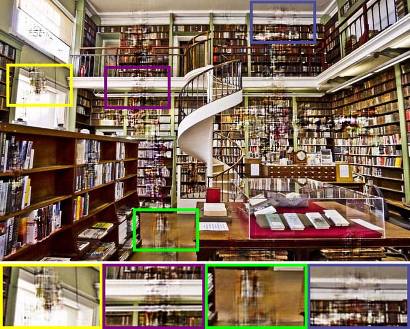
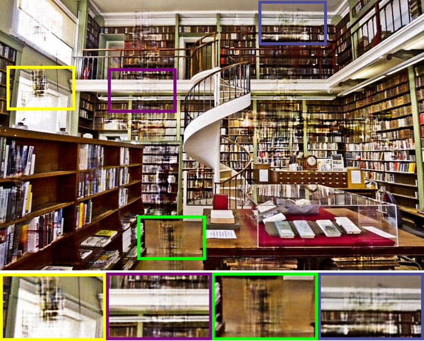
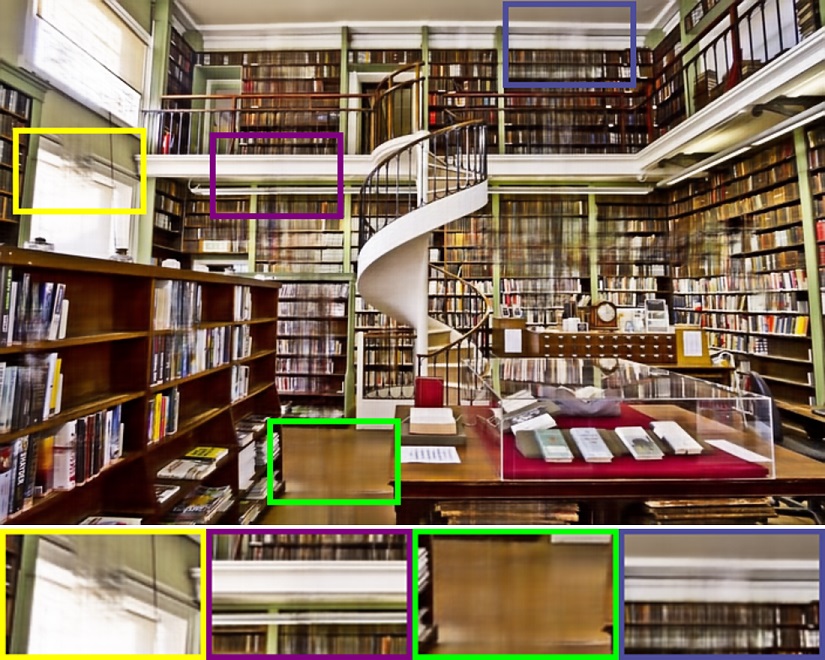
(a) Input	(b) SGD (19.23 dB)	(c) SGD + Input (19.59 dB)	(d) SGLD mean (21.86 dB)

Figure 5: (Best viewed magnified.) Image inpainting using the deep image prior. The posterior mean using SGLD (Panel (d)) achieves higher PSNR values and has fewer artifacts than SGD variants. See the Appendix for more comprisons.

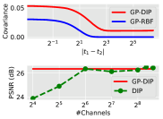
(a)	(b) GT	(c) Corrupted	(d) GP RBF (25.78)	(e) GP DIP (26.34)	(f) DIP (26.43)

Figure 6: Inpainting with a Gaussian process (GP) and deep image prior (DIP). Top (a) Comparison of the Radial basis function (RBF) kernel with the length scale learned on observed pixels in (c) and the stationary DIP kernel. Bottom (a) PSNR of the GP posterior with the DIP kernel and DIP as a function of the number of channels. DIP approaches the GP performance as the number of channels increases from 16 to 512. (d - f) Inpainting results (with the PSNR values) from GP with the RBF (GP RBF) and DIP (GP DIP) kernel, as well as the deep image prior. The DIP kernel is more effective than the RBF.

The above figure shows two samples each drawn from the DIP (with 256 channels per layer) and GP with the equivalent kernel. The samples are nearly identical suggesting that the characterization of the DIP as a stationary GP also holds for 2D signals. Next, we compare the DIP and GP on an inpainting task shown in Figure 6. The image size here is 64$\times$64. Figure 6 top (a) shows the RBF and DIP kernels as a function of the offset. The DIP kernels are heavy tailed in comparison to Gaussian with support at larger length scales. Figure 6 bottom (a) shows the performance (PSNR) of the DIP as a function of the number of channels from 16 to 512 in each layer of the U-Net, as well as of a GP with the limiting DIP kernel. The PSNR of the DIP approaches the GP as the number of channels increases suggesting that for networks of this size 256 filters are enough for the asymptotic GP behavior. Figure 6 (d-e) show that a GP with the DIP kernel is more effective than one with the RBF kernel, suggesting that the long-tail DIP kernel is better suited for modeling natural images.

While DIPs are asymptotically GPs, the SGD optimization may be preferable because GP inference is expensive for high-resolution images. The memory usage is $O(n^{2})$ and running time is $O(n^{3})$ for exact inference where $n$ is the number of pixels (e.g., a 500$\times$500 image requires 233 GB memory). The DIP’s memory footprint, on the other hand, scales linearly with the number of pixels, and inference with SGD is practical and efficient. This emphasizes the importance of SGLD, which addresses the drawbacks of vanilla SGD and makes the DIP more robust and effective. Finally, while we showed that the prior distribution induced by the DIP is asymptotically a GP and the posterior estimated by SGD or SGLD matches the GP posterior for small networks, it remains an open question if the posterior matches the GP posterior for deeper networks.

6 Conclusion

We presented a novel Bayesian view of the deep image prior, which parameterizes a natural image as the output of a convolutional network with random parameters and a random input. First, we showed that the output of a random convolutional network converges to a stationary zero-mean GP as the number of channels in each layer goes to infinity, and showed how to calculate the realized covariance. This characterized the deep image prior as approximately a stationary GP. Our work differs from prior work relating GPs and neural networks by analyzing the spatial covariance of network activations on a single input image. We then use SGLD to conduct fully Bayesian posterior inference in the deep image prior, which improves performance and prevents the need for early stopping. Future work can further investigate the types of kernel implied by convolutional networks to better understand the deep image prior and the inductive bias of deep convolutional networks in learning applications.

Acknowledgement

This research was supported in part by NSF grants #1749833, #1749854, and #1661259, and the MassTech Collaborative for funding the UMass GPU cluster.

Appendix

We provide the proof of Theorem 1 and show additional visualizations of the denoising and inpainting results.

Proof.

Let $r=t_{2}-t_{1}$. First, observe that

$$\begin{split}\bar{x}(t_{1})^{T}\bar{x}(t_{2})=\sum_{k=1}^{n}\bigg{(}\sum_{i=0}^{d-1}x(k,t_{1}-i)x(k,t_{2}-i)\bigg{)}.\\ \end{split}$$

where $n$ is the number of channels in the input, $d$ is the filter width. By stationarity, the terms $x(k,t_{1}-i)x(k,t_{2}-i)$ are identically distributed with expected value $K_{x}(r)$, even though they are not necessarily independent. Since the channels are drawn independently, the parenthesized expressions in the sum over $k$ are iid with mean $dK_{x}(r)$. According to Equation 2 in the main text, we have

$$K_{z}^{\rm erf}(t_{1},t_{2}) =\mathbb{E}_{x}V_{\rm erf}\big{(}\bar{x}(t_{1}),\bar{x}(t_{2})\big{)}$$

$$=\mathbb{E}_{x}\frac{2}{\pi}\sin^{-1}\frac{\sigma^{2}_{u}\bar{x}(t_{1})^{T}\bar{x}(t_{2})}{\sigma^{2}_{u}\|\bar{x}(t_{1})\|\|\bar{x}(t_{2})\|}.$$

Consider the sequence $Y_{n}=(a_{n},b_{n},c_{n})$

$$\begin{split}a_{n}&=\frac{1}{n}\left(\bar{x}(t_{1})^{T}\bar{x}(t_{2})\right)\\ b_{n}&=\frac{1}{n}\left(\bar{x}(t_{1})^{T}\bar{x}(t_{1})\right)\\ c_{n}&=\frac{1}{n}\left(\bar{x}(t_{2})^{T}\bar{x}(t_{2})\right),\end{split}$$

By the strong law of large numbers we know the sequences $a_{n}$, $b_{n}$ and $c_{n}$ each converge almost surely to their expected values $dK_{x}(t_{1},t_{2})$, $dK_{x}(t_{1},t_{1})$ and $dK_{x}(t_{2},t_{2})$, respectively. Since $K_{x}$ is stationary this is equal to $dK_{x}(r)$, $dK_{x}(0)$, and $dK_{x}(0)$, respectively, where $d$ is the filter width. Thus we have that $Y_{n}$ converges almost surely to $\bar{y}=\big{(}dK_{x}(r),dK_{x}(0),dK_{x}(0)\big{)}$.

Consider the continuous function $g(y)=\frac{2}{\pi}\sin^{-1}\left(\frac{a}{\sqrt{bc}}\right)$ for $y=(a,b,c)$. Applying the continuous mapping theorem, we have that

$$y_{n}\xrightarrow{a.s.}\mu\;\implies\;g(y_{n})\xrightarrow{a.s.}g(\mu)$$

Thus,

$$K_{z}^{\rm erf}(t_{1},t_{2})\xrightarrow{a.s.}\frac{2}{\pi}\sin^{-1}\frac{K_{x}(r)}{K_{x}(0)}.$$

∎

Additional visualizations.

Figure 7 and 8 present results for various inputs using various inference schemes for image denoising and image inpainting respectively.

(a) GT	(b) Noisy GT	(c) SGD	(d) +Avg	(e) +Input	(f) +Input+Avg	(g) SGLD
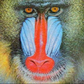
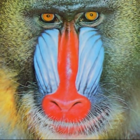
	20.34	23.81	23.94	22.52	23.52	24.59
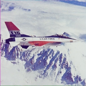
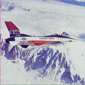
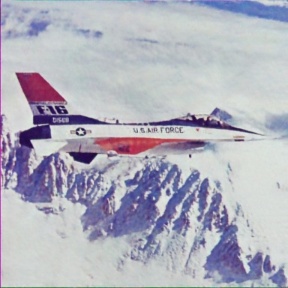
	20.33	29.81	31.12	30.65	32.73	32.95
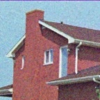
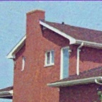
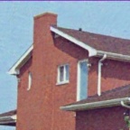
	20.28	26.14	28.59	27.92	30.37	31.32
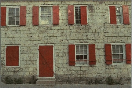
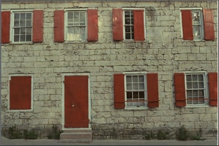
	20.28	26.67	27.16	26.28	27.25	27.95
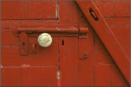
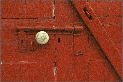
	20.57	28.77	29.87	30.30	31.74	32.05
	20.36	30.23	31.02	31.34	32.84	33.39
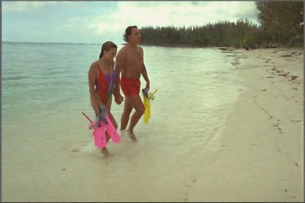
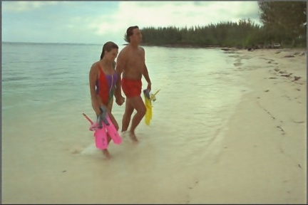
	20.32	29.62	30.46	30.84	32.07	32.81
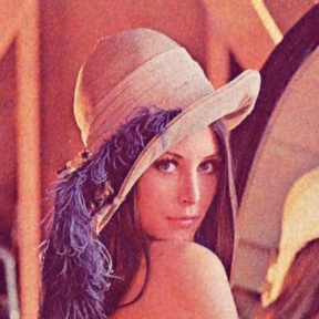
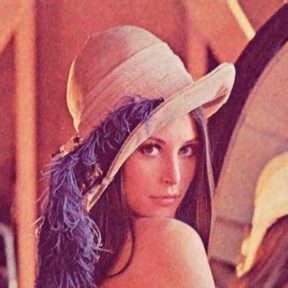
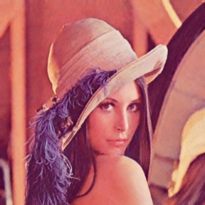
	20.37	29.07	30.28	30.21	31.81	32.08

Figure 7: (Best viewed magnified.) Comparison of inference schemes for image denoising. From left to right each column shows (a) ground truth image, (b) the ground truth image corrupted with Gaussian noise of $\sigma=25$, (c) inference with SGD and early stopping (iteration picked at maximum PSNR), (d) previous step with exponential window average, (e) SGD with input noise and early stopping, (f) the previous procedure with exponential window averaging, and (g) SGLD. Underneath each figure the PSNR values are listed. Note that except SGLD every procedure requires early stopping.

References

- [1] David Barber and Christopher Bishop. Ensemble Learning in Bayesian Neural Networks. In Generalization in Neural Networks and Machine Learning, pages 215–237. Springer Verlag, January 1998.
- [2] Charles Blundell, Julien Cornebise, Koray Kavukcuoglu, and Daan Wierstra. Weight Uncertainty in Neural Network. In International Conference on Machine Learning, pages 1613–1622, 2015.
- [3] Anastasia Borovykh. A Gaussian Process Perspective on Convolutional Neural Networks. arXiv:1810.10798, 2018.
- [4] Antoni Buades, Bartomeu Coll, and J-M Morel. A Non-local Algorithm for Image Denoising. In IEEE Conference on Computer Vision and Pattern Recognition, 2005.
- [5] Youngmin Cho and Lawrence K Saul. Kernel Methods for Deep Learning. In Advances in Neural Information Processing Systems, pages 342–350, 2009.
- [6] Kostadin Dabov, Alessandro Foi, Vladimir Katkovnik, and Karen Egiazarian. Image Denoising by Sparse 3-D Transform-domain Collaborative Filtering. IEEE Transactions on image processing, 16(8):2080–2095, 2007.
- [7] John S Denker and Yann LeCun. Transforming Neural-net Output Levels to Probability Distributions. In Advances in Neural Information Processing Systems, pages 853–859, 1991.
- [8] Yarin Gal and Zoubin Ghahramani. Dropout as a Bayesian Approximation: Representing Model Uncertainty in Deep Learning. In International Conference on Machine Learning, pages 1050–1059, 2016.
- [9] Adrià Garriga-Alonso, Laurence Aitchison, and Carl Edward Rasmussen. Deep Convolutional Networks as Shallow Gaussian Processes. arXiv:1808.05587, 2018.
- [10] Alex Graves. Practical Variational Inference for Neural Networks. In Advances in Neural Information Processing Systems, pages 2348–2356, 2011.
- [11] Felix Heide, Wolfgang Heidrich, and Gordon Wetzstein. Fast and Flexible Convolutional Sparse Coding. In Computer Vision and Pattern Recognition (CVPR), 2015.
- [12] Geoffrey E Hinton and Drew Van Camp. Keeping the Neural Networks Simple by Minimizing the Description Length of the Weights. In Conference on Computational Learning Theory, pages 5–13. ACM, 1993.
- [13] Jaehoon Lee, Yasaman Bahri, Roman Novak, Sam Schoenholz, Jeffrey Pennington, and Jascha Sohl-dickstein. Deep Neural Networks as Gaussian Processes. International Conference on Learning Representations, 2018.
- [14] Chunyuan Li, Changyou Chen, David E Carlson, and Lawrence Carin. Preconditioned Stochastic Gradient Langevin Dynamics for Deep Neural Networks. In AAAI, volume 2, page 4, 2016.
- [15] David JC MacKay. A Practical Bayesian Framework for Backpropagation Networks. Neural computation, 4(3):448–472, 1992.
- [16] Henry B Mann and Abraham Wald. On Stochastic Limit and Order Relationships. The Annals of Mathematical Statistics, 14(3):217–226, 1943.
- [17] Georges Matheron. The Intrinsic Random Functions and Their Applications. Advances in applied probability, 5(3):439–468, 1973.
- [18] Alexander G de G Matthews, Mark Rowland, Jiri Hron, Richard E Turner, and Zoubin Ghahramani. Gaussian Process Behaviour in Wide Deep Neural Networks. arXiv:1804.11271, 2018.
- [19] Radford M Neal. Bayesian Learning for Neural Networks. PhD thesis, University of Toronto, 1995.
- [20] Roman Novak, Lechao Xiao, Yasaman Bahri, Jaehoon Lee, Greg Yang, Jiri Hron, Daniel A Abolafia, Jeffrey Pennington, and Jascha Sohl-Dickstein. Bayesian Deep Convolutional Networks with Many Channels are Gaussian Processes. In International Conference on Learning Representations, 2019.
- [21] Vardan Papyan, Yaniv Romano, Michael Elad, and Jeremias Sulam. Convolutional Dictionary Learning via Local Processing. In International Conference on Computer Vision, pages 5306–5314, 2017.
- [22] Carl Edward Rasmussen. Evaluation of Gaussian Processes and Other Methods for Non-linear Regression. University of Toronto, 1999.
- [23] Carl Edward Rasmussen. Gaussian Processes in Machine Learning. In Advanced lectures on machine learning, pages 63–71. Springer, 2004.
- [24] Andrew M. Saxe, Pang Wei Koh, Zhenghao Chen, Maneesh Bhand, Bipin Suresh, and Andrew Y. Ng. On Random Weights and Unsupervised Feature Learning. In International Conference on Machine Learning, 2011.
- [25] Charles W Therrien. Issues in Multirate Statistical Signal Processing. In Signals, Systems and Computers, 2001. Conference Record of the Thirty-Fifth Asilomar Conference on, volume 1, pages 573–576. IEEE, 2001.
- [26] Dmitry Ulyanov, Andrea Vedaldi, and Victor Lempitsky. Deep Image Prior. In Computer Vision and Pattern Recognition (CVPR), 2018.
- [27] Ivan Ustyuzhaninov, Wieland Brendel, Leon A Gatys, and Matthias Bethge. Texture Synthesis using Shallow Convolutional Networks with Random Filters. arXiv:1606.00021, 2016.
- [28] Max Welling and Yee W Teh. Bayesian Learning via Stochastic Gradient Langevin Dynamics. In International Conference on Machine Learning, 2011.
- [29] Christopher KI Williams. Computing with Infinite Networks. In Advances in Neural Information Processing Systems, 1997.
- [30] Christopher KI Williams and David Barber. Bayesian Classification with Gaussian Processes. IEEE Transactions on Pattern Analysis and Machine Intelligence, 20(12):1342–1351, 1998.
- [31] Christopher K. I. Williams and Carl Edward Rasmussen. Gaussian Processes for Regression. In Advances in Neural Information Processing Systems, pages 514–520, 1996.