Exotic coloured fermions and lepton number violation at the LHC

Abstract

Majorana neutrino mass models with a scale of lepton number violation (LNV) of order TeV potentially lead to signals at the LHC. Here, we consider an extension of the standard model with a coloured octet fermion and a scalar leptoquark. This model generates neutrino masses at 2-loop order. We make a detailed MonteCarlo study of the LNV signal at the LHC in this model, including a simulation of standard model backgrounds. Our forecast predicts that the LHC with 300/fb should be able to probe this model up to colour octet fermion masses in the range of (2.6-2.7) TeV, depending on the lepton flavour of the final state.

I Introduction

All Majorana neutrino mass models with a scale of lepton number violation (LNV) of roughly $\Lambda_{LNV}\sim{\cal O}$(TeV) can lead to lepton number violating signals at the LHC. The best-known example is the left-right symmetric extension of the standard model Pati:1974yy ; Mohapatra:1974gc ; Mohapatra:1980yp . Here, right-handed $W_{R}$ boson production can lead to the final states $\ell^{\pm}\ell^{\pm}jj$ and $\ell^{\pm}\ell^{\mp}jj$ Keung:1983uu .

There are, however, many other possible electro-weak scale extensions of the standard model that potentially lead to LNV signals at the LHC. In particular, the systematic analysis of the short-range contributions to neutrinoless double beta decay Bonnet:2012kh has found a variety of such models, all of which can in principle explain neutrino oscillation data. (For a recent global fit of all oscillation data see, for example deSalas:2017kay .) Rough estimates of the LHC reach, compared with the sensitivity of current and future double beta decay experiments, have been made in Helo:2013dla ; Helo:2013ika ; Gonzales:2016krw . In this paper, we study LHC signals for a particularly simple LNV extension of the SM. This model generates neutrino masses at 2-loop order and, thus, one expects the masses of the exotic particles of this model to be at least partially within reach of the LHC. Different from previous papers Helo:2013dla ; Helo:2013ika ; Gonzales:2016krw , here we perform a full detector simulation and background study, in order to give more realistic estimates for future LHC sensitvities.

Only very few searches for LNV final states at the LHC exist so far. CMS Khachatryan:2014dka has searched for same-sign dileptons plus jets in 8 TeV data. The results were interpreted as lower limits on the mass of $W_{R}$ as function of right-handed neutrino mass. Lower limits on $m_{W_{R}}$ approaching 3 TeV have been derived, for $m_{N}<m_{W_{R}}$ and assuming the gauge coupling of the right-handed bosons to be equal to the standard model $SU(2)_{L}$ coupling. A small excess around $p^{2}_{\ell\ell jj}=2$ TeV was observed (statistically with a local significance of 2.8 $\sigma$), but discarded by the experimentalists as a signal, since the sample consists dominantly of opposite sign lepton final states. (See, however, the discussion in Anamiati:2016uxp .) Unfortunately, the recent update of this search by CMS Sirunyan:2018pom with $\sqrt{s}=13$ TeV data, could not reproduce this excess and now quotes a lower limit of $m_{W_{R}}\geq 4.4$ TeV. A very similar search by ATLAS Aaboud:2018spl has also been published, providing lower limits extending up to $m_{W_{R}}\geq 4.7$ TeV, for $m_{N}\raise 1.29167pt\hbox{$\;<$\kern-7.5pt\raise-4.73611pt\hbox{$\sim\;$}}m_{W_{R}}/2$.

We also want to mention that for models with a seesaw type-II, pair production of the doubly charged component of the triplet can lead to $\Delta^{++}\Delta^{--}\to\ell^{\pm}\ell^{\pm}W^{\mp}W^{\mp}\to\ell^{\pm}\ell^{\pm}+4j$ Azuelos:2004mwa ; Perez:2008ha ; Melfo:2011nx . If only leptonic or $WW$ final states were observed, LNV could not be established at the LHC, but the type of scalar multiplet could still be determined delAguila:2013yaa . However, no search for $\ell^{\pm}\ell^{\pm}W^{\mp}W^{\mp}$ at the LHC exists so far. Instead, ATLAS Aaboud:2017qph searched for $pp\to\Delta^{++}\Delta^{--}\to 4\ell$. For a doubly charged Higgs boson only coupling to left-handed leptons, the limits vary from (770 - 870) GeV, depending on the lepton flavour, assuming Br($\Delta^{\pm\pm}\to\ell^{\pm}_{\alpha}\ell^{\pm}_{\beta}$) equal to 1 (for $\alpha,\beta=e,\mu$). ATLAS Aaboud:2018qcu has also searched for $pp\to\Delta^{++}\Delta^{--}\to 4W$. However, lower limits, based on 36.1/fb, are currently only of order 220 GeV.

The model we consider in this paper contains two new particles: A scalar leptoquark (LQ) and an exotic colour-octet fermion, $\Psi$ (for details see section II). The fermion can be pair-produced, decaying to the final state $\ell^{\pm}jj$. We will discuss restrictions on the fermion in this model from the searches Sirunyan:2018pom ; Aaboud:2018spl in section IV. As for the leptoquark, currently the best limits come from CMS Sirunyan:2018btu and ATLAS Aaboud:2019jcc . CMS Sirunyan:2018btu finds lower limits on pair-produced leptoquarks, giving $m_{LQ}\geq 1435$ ($1270$) GeV for a branching ratio of $\mbox{Br}(S_{LQ}\to\ell^{\pm}j)=1$ ($0.5$). ATLAS derives Aaboud:2019jcc a very similar number of $m_{LQ}\geq 1.25$ TeV for a branching ratio equal to 0.5.

In order to estimate the reach of our model for the LHC Run-3, we performed detector level studies of the same-sign dilepton plus four jets final state. In section III the MonteCarlo simulation and the cut and count analysis optimization are discussed in some detail. Signal and SM background $H_{T}$ distributions are shown and the corresponding yield tables after the selection cuts are included for completeness in the appendix (section VI). In section IV, our results are presented as the $2\sigma$ limits and $5\sigma$ discovery regions, forecasted for the $\Psi\rightarrow\ell^{\pm}jj$ branching ratio, with $\ell=e,\mu$, as a function of the colour octet fermion mass.

The rest of this paper is organized as follows: in section II we describe the model basics, discuss briefly non-LHC constraints, such as neutrino masses, and describe the benchmark scenarios we use in the rest of the paper. In section III the MonteCarlo simulation is discussed and our results are presented in section IV. In section V the conclusions and outlook of this work are given.

II Model Basics

In this paper, we use a particularly simple 2-loop neutrino mass model. The model adds only two new particles to the standard model: A (singlet) scalar leptoquark $S_{LQ}\equiv S_{3,1,-1/3}$ and a colour octet fermion, $\Psi\equiv\Psi_{8,1,0}$. Here the subscripts denote the transformation properties/charge under the SM gauge group, $SU(3)_{c}\times SU(2)_{L}\times U(1)_{Y}$. We note that this model has appeared twice in the literature before. It was listed in Bonnet:2012kh as one particular example of a short-range contribution to neutrinoless double beta decay. And in Angel:2013hla predictions for neutrino masses and low energy lepton flavour violation for this model have been worked out in detail.

With these new fields the lagrangian of the model contains the following terms:

$${\cal L} = (Y_{1})_{\alpha\beta}\overline{L^{c}}_{\alpha}Q_{\beta}S^{\dagger}_{LQ}+(Y_{2})_{\alpha\beta}\overline{d_{R}}_{\alpha}\Psi_{\beta}S_{LQ}+(Y_{3})_{\alpha\beta}\overline{e_{R}^{c}}_{\alpha}u_{R,\beta}S^{\dagger}_{LQ}+h.c.$$

$$+ \frac{1}{2}m_{\Psi}\bar{\Psi}^{c}\Psi+m_{LQ}^{2}S^{\dagger}_{LQ}S_{LQ}+\cdots$$

Here $\alpha$ and $\beta$ are generation indices and we have left open the possibility that more than one copy of $\Psi$ could exist. The quantum numbers of the scalar leptoquark $S_{LQ}$ allow, in principle, to write down two more terms in the lagrangian, $\bar{Q}Q^{c}S_{LQ}$ and $\bar{u}d^{c}S_{LQ}^{\dagger}$. These, if coupled to the first generation of quarks, induce rapid proton decay. As noted in Baldes:2011mh , stringent upper limits on Yukawa couplings in any quark generation indices can be derived from the requirement of successful baryogenesis. In order to avoid these problems, we simply postulate baryon-number conservation as an additional symmetry of the model.

Figure 1: 2-loop neutrino mass diagram for the model considered in this work.

The main motivation for studying this model is that it can explain neutrino oscillation data by generating neutrino masses at 2-loop level as shown in figure (1). Assuming only one copy of $\Psi$ this diagram gives a contribution to the neutrino mass matrix, roughly as Angel:2013hla ; deGouvea:2007xp ; Sierra:2014rxa

$$(m_{\nu})_{\alpha\beta}\sim\frac{N_{c}}{(16\pi^{2})^{2}}\frac{m_{\Psi}}{m_{LQ}^{2}}\Big{[}(Y_{1})_{\alpha k}(Y_{2})_{k}m_{k}I_{kr}(x^{2})m_{r}(Y_{2})_{r}(Y_{1})_{\beta r}+\alpha\leftrightarrow\beta\Big{]}.$$ (2)

Here, $N_{c}$ is a color factor, $m_{k}$ and $m_{r}$ are down quark masses of generation $k,r$ and $I_{kr}(x^{2})$ stands for the 2-loop integral Angel:2013hla ; Sierra:2014rxa , with the dimensionless argument $x=(m_{\Psi}/m_{LQ})$. Note that with the quark masses much smaller than the mass of $\Psi$ and $S_{LQ}$, $I_{kr}(x^{2})$ is to a good approximation independent of $k$ and $r$, i.e. $I(x^{2})$. In order to reproduce the neutrino mass, estimated from the atmospheric neutrino masss scale ($m_{\nu}\sim 0.05$ eV), and assuming very roughly $m_{\Psi}\sim m_{LQ}\sim\Lambda_{LNV}\sim{\cal O}$(TeV), the Yukawa couplings (for third generation quarks) in eq. (2) should be of order (few) ${\cal O}(10^{-2})$.

Since neutrino mass models must not only produce the correct absolute value of one neutrino mass, but also reproduce the solar mass scale and the observed flavour structure of the neutrino mass matrix, the above estimate is only indicative of the typical size of parameters. On closer inspection, one sees that in the limit where only $m_{b}$ is taken different from zero, eq. (2) generates only one neutrino mass. The authors of Angel:2013hla therefore suggested to use two copies of $S_{LQ}$. However, we note that contributions proportional to $m_{s}$, while being smaller than those proportional to $m_{b}$, could generate a large enough second neutrino mass, if the entries in the Yukawa matrices $Y_{1}$ and $Y_{2}$ for 2nd generation quarks are roughly larger, by a factor $\sqrt{m_{b}/m_{s}}\sim 6$ each, than those for 3rd generation quarks. Also, the fit of non-zero neutrino angles requires flavor off-diagonal entries in $(m_{\nu})_{\alpha\beta}$, implying lepton flavour violating charged lepton decays. We will not repeat this discussion here, since a detailed study can be found in Angel:2013hla .

Lepton number violation in this model is due to the Majorana mass term $m_{\Psi}$. $\Psi$, once produced, can decay to a down quark and $S_{LQ}$. Since $\Psi$ is a Majorana fermion, decays to $\overline{d_{R}}S_{LQ}$ and $d_{R}S_{LQ}^{\dagger}$ are equally likely. Thus, pair-produced $\Psi$ will lead to the LNV and LNC final states $\ell^{\pm}_{\alpha}\ell^{\pm}_{\beta}+4j$ and $\ell^{\pm}_{\alpha}\ell^{\mp}_{\beta}+4j$, as shown in figure (2). There are, however, some important differences to the case of the type-II seesaw discussed in the introduction. First, $\Psi$ being a colour octet, production cross sections are much larger in the current model. And, second, in type-II seesaw the invariant masses of the subsystems $\ell^{\pm}_{\alpha}\ell^{\pm}_{\beta}$ and $4j$ should both equal the mass of $\Delta^{++}$. Here, on the other hand, the invariant masses of two particular $\ell jj$ subsets should produce mass peaks. As discussed in Helo:2013ika , if a discovery of LNV is eventually made at the LHC, this can be used to distinguish different models.

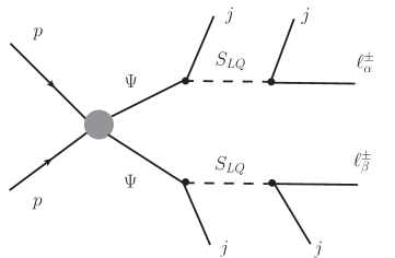
Figure 2: Pair production of the colour-octet fermion $\Psi$, followed by 3-body decays, at the LHC.

More important for our forecasts is, however, that the information from neutrino oscillation experiments is not sufficient to fix all entries in the Yukawa matrices $Y_{1,2,3}$. The large mixing angles observed indicate that lepton flavour violating final states should likely be large in $\ell^{\pm}_{\alpha}\ell^{\pm}_{\beta}+4j$. On the other hand, the sensitivity of the LHC to final states involving tau leptons is markedly less than for muons or electrons. We thus decided to consider in our numerical studies only three simple benchmark scenarios for the Yukawa couplings. These are:

1. The scalar leptoquark couples to electrons only, i.e., $(Y_{1})_{\mu\beta}=(Y_{1})_{\tau\beta}=(Y_{3})_{\mu\beta}=(Y_{3})_{\tau\beta}=0$.

2. The scalar leptoquark couples to muons only, i.e., $(Y_{1})_{e\beta}=(Y_{1})_{\tau\beta}=(Y_{3})_{e\beta}=(Y_{3})_{\tau\beta}=0$.

3. The scalar leptoquark couples to electrons and muons (no taus) with the same rate, i.e., $(Y_{1})_{\mu}=(Y_{1})_{e}$, $(Y_{3})_{\mu\beta}=(Y_{3})_{e\beta}$ with $(Y_{1})_{\tau\beta}=(Y_{3})_{\tau\beta}=0$.

Couplings to the 3rd generation quarks could be sizeable, leading to final states involving bottom or even top quarks. However, we will limit ourselves in this paper to the study of light quarks, i.e. we consider only jets without any flavour tags for the quarks.

We close this section with the short comment that a number of similar LNV models can easily be constructed, all of which lead in principle to the same LHC signal. In fact, the model we have considered in this section corresponds to a particular example of a $d=9$ short-range neutrinoless double beta decay operator decomposition that generates neutrino masses at 2-loop. As can be seen in Table IV of ref. Helo:2015fba , all models in this class have an exotic coloured fermion that might be pair produced at the LHC.

III Montecarlo Simulation

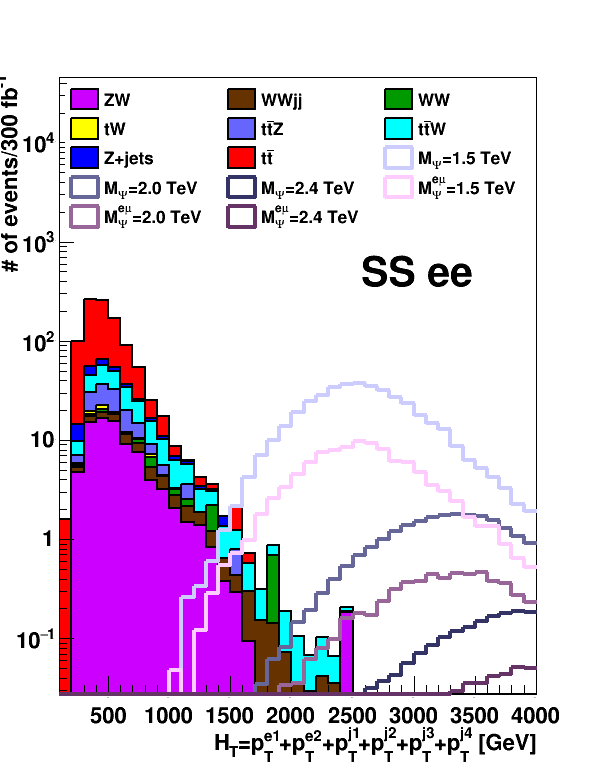
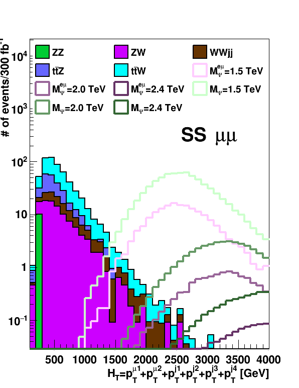
Figure 3: Signal (solid lines) and SM background (stacked histograms) $H_{T}^{ll}$ distributions after the pre-selection cuts described in the text are applied. Signal samples for the $ee$ (left), $\mu\mu$ (right) and $e\mu$ (both plots) scenarios are shown. Only a few signal mass points are shown for the sake of clarity.

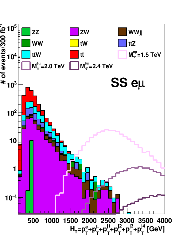
Figure 4: Signal (solid lines) and SM background (stacked histograms) $H_{T}^{e\mu}$ distributions after the pre-selection cuts described in the text are applied. Only a few signal mass points are shown for the sake of clarity.

In order to estimate the sensitivity reach of our model at the LHC Run-3 (i.e. an integrated luminosity of 300/fb and a center of mass energy of $\sqrt{s}=13$ TeV), we have performed realistic detector level simulations of the same-sign (SS) dilepton plus four hard jets final state signal, shown in figure (2), as well as of the most relevant SM backgrounds. Our signals correspond to the three benchmark scenarios described in section II with the mass of the colour octet fermion $m_{\Psi}$ varying in the range [1.5, 2.9] TeV, while the scalar leptoquark mass is supposed to always be larger than $m_{\Psi}$, and is therefore off-shell in the $\Psi$ decay. Signal and SM background events were generated at parton level using Madgraph5 v2.3.3 Alwall:2011uj .

For the simulation of the signal, we have written a private model file and implemented it in SARAH Staub:2012pb ; Staub:2013tta . SARAH then allows to generate automatically a version of SPheno Porod:2003um ; Porod:2011nf , with which a numerical calculation for different observables, such as masses and decay branching ratios can be done.

For the SM processes, we used the built-in model available in MadGraph, including the following backgrounds $t\bar{t},Z,W^{\pm}W^{\pm},ZZ,ZW^{\pm},W^{\pm}W^{\mp},t\bar{t}Z,t\bar{t}W^{\pm}$ plus 2-4 additional final state partons and $Z$, $W$ and $t$ decaying to leptons ($e,\mu$). Parton showers and particle decays were generated with Pythia 6.4 Sjostrand:2000wi ; Sjostrand:2006za and the matrix element to parton shower matching procedure (MLM) was implemented when generating SM background processes in order to avoid double counting of the radiated partons. The interaction of final state particles with the detector and their reconstruction was simulated using Delphes 3 Ovyn:2009tx , configured to replicate the ATLAS detector layout and its performance. Jets were reconstructed with the anti-$k_{t}$ algorithm using a cone size of $R=0.4$. Note that most of the SM background processes listed above produce opposite-sign (OS) dilepton final states, while we consider only SS dilepton final states in our analysis. We must include these processes when we have final states containing electrons, due to the charge flip effect. We expect indeed a significant OS event contamination into the SS region. In order to account for this effect in final states containing electrons, we reweighted our events using the charge flip probability measured by ATLAS (see figure 2a. of TheATLAScollaboration:2013jha ), parametrized in electron $p_{T}$ and $\eta$. We did not consider background contributions from QCD-jets faking leptons in our analysis, since we expect these to be negligible for very high-$p_{T}$ electrons and muons, as those produced in our signal.

In order to validate our simulated SM backgrounds against measured quantities, we used those already performed at the LHC Run 2 by ATLAS and compared the simulated distribution of number of jets for $t\bar{t}$ and $Z+jets$, with the measurements performed in Aaboud:2016pbd and Aaboud:2017hbk , respectively. After a simple linear rescaling of the simulated distributions to the partial Run 2 luminosities, and applying the selection cuts used in those studies, we compared our number of jets distributions with the distributions measured by ATLAS and derived the correction factors needed to account for the observed differences. The correction was applied to our simulated $Z+jets$ and $t\bar{t}$ samples as a function of the number of jets, before the pre-selection used in this analysis. Other samples were not corrected in this way since the corresponding measurements were not available. The pre-selection cuts we applied were similar for all final states considered:

1. A pair of same-sign (SS) reconstructed leptons with $p_{T}>20$ GeV.

2. In the case of $ee$ final state, we also require the dilepton mass to be larger than $110$ GeV, in order to further suppress $Z+jets$ background.

3. At least four jets are required, each of them satisfying $p_{T}^{j}>20$ GeV.

As a discriminating variable we used the scalar sum of the hardest leptons and jets in the event, $H_{T}\equiv p_{T}^{\ell_{1}}+p_{T}^{\ell_{2}}+p_{T}^{j_{1}}+p_{T}^{j_{2}}+p_{T}^{j_{3}}+p_{T}^{j_{4}}$. We found the significance is larger when using $H_{T}$ compared with $m_{\ell jj}$ or $m_{\ell\ell jjjj}$ invariant mass distributions, which are both affected by a large combinatorial background, due to the many ways the jets can be paired with the leptons. $H_{T}$ distributions after pre-selection for $ee$, $\mu\mu$ are shown in figure (3) and $e\mu$ in figure (4).

IV Results

In this section, we use the results from section III to estimate future limits on the $\Psi\rightarrow\ell jj$ ($\ell=e,\mu$) branching fraction, for each of the benchmark scenarios described in section II. Figures (3) and (4) show the number of signal and background events, before the $H_{T}$ cut, for the $e^{\pm}e^{\pm}jjjj$, $\mu^{\pm}\mu^{\pm}jjjj$ and $e^{\pm}\mu^{\pm}jjjj$ final states. Depending on the final state, the signals are shown for the scenarios where the scalar leptoquark couples to electrons only ($ee$), muons only ($\mu\mu$), or to electrons and muons with the same strength ($e\mu$).

While the $ee$ ($\mu\mu$) scenario is constrained by the $e^{\pm}e^{\pm}jjjj$ ($\mu^{\pm}\mu^{\pm}jjjj$) final state only, the $e\mu$ scenario is constrained by the three final states: $e^{\pm}e^{\pm}jjjj$, $\mu^{\pm}\mu^{\pm}jjjj$ and $e^{\pm}\mu^{\pm}jjjj$. For an off-shell scalar leptoquark ($S_{LQ}$), the number of signal events is given by

$$S=\sigma(gg\rightarrow\Psi\Psi)\times\mbox{Br}(\Psi\rightarrow\ell jj)\times\mbox{Br}(\Psi\rightarrow\ell^{\prime}jj)\times\mathcal{L}_{int}\times\eta,$$ (3)

where $\ell,\ell^{\prime}=e,\mu$, $\mathcal{L}_{int}=300\mbox{ fb}^{-1}$ and $\eta$ is our cut efficiency. (See the discussion in the previous section and the tables in the appendix.)

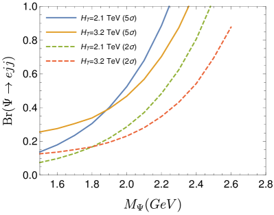
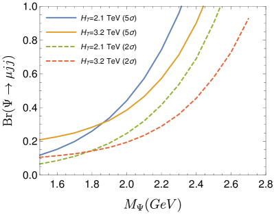
Figure 5: Minimum $\mbox{Br}(\Psi\rightarrow\ell jj)$ for discovery (solid lines) and $2\sigma$-limits (dashed lines) as a function of $m_{\Psi}$, for two values of the $H_{T}$ cut. Left for $\ell=e$ (in the scenario where the scalar leptoquark couples to electrons only) and right for $\ell=\mu$ (in the scenario where the scalar leptoquark couples to muons only). The red dashed line does not reach $\mbox{Br}=1$, because we restrict the curves to regions with more than one signal event.

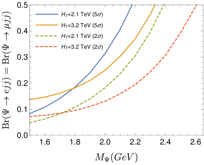
Figure 6: Minimum $\mbox{Br}(\Psi\rightarrow ejj)=\mbox{Br}(\Psi\rightarrow\mu jj)$ for discovery (solid lines) and $2\sigma$-limits (dashed lines) as a function of $m_{\Psi}$, for two values of the $H_{T}$ cut, in the scenario where the scalar leptoquark couples to electrons and muons with the same strength.

The number of signal events for both the $ee$ and $\mu\mu$ scenarios were obtained assuming $\mbox{Br}(\Psi\rightarrow\ell jj)=1$, while for the $e\mu$ scenario we assumed $\mbox{Br}(\Psi\rightarrow ejj)=\mbox{Br}(\Psi\rightarrow\mu jj)=1/2$. In order to find the discovery reach and forecasted limits, we scale these results accordingly and find the minimum value of the branching ratio required to get a $5\sigma$ or $2\sigma$ significance. For the significance, $Z$, we use the expression:

$$Z=\sqrt{2\left[(S+B)\times\ln\left(1+\frac{S}{B}\right)-S\right]},$$ (4)

where $S$ is the number of signal events and $B$ is the number of background events. We restrict our analysis to regions with at least one signal event.

Our results are shown in figures (5) and (6). The three different plots correspond to the three different scenarios previously discussed: $ee$, $\mu\mu$ and $e\mu$. In each plot, we show the minimum branching fraction for $5\sigma$-discovery (solid lines) and $2\sigma$-limits (dashed lines) as a function of the mass of the colour-octet fermion $\Psi$. From these plots one can see that larger values of the $H_{T}$ cut give better sensitivities in regions of parameter space with larger values of $m_{\Psi}$ (removing most of the backgrounds), while lower values of $H_{T}$ are better for smaller values of $m_{\Psi}$. For this reason, for each scenario we show our results for two different values of the $H_{T}$ cut. As expected, for high (low) masses the expected limits are stronger (weaker) for lower (higher) values of $H_{T}$. Depending on the scenario, the LHC with 300/fb should be able to discover (give limits for) the colour octet fermion with masses in the range $2.3-2.4$ TeV ($2.6-2.7$ TeV).

Before closing, we want to briefly discuss the LNV searches by CMS Sirunyan:2018pom and ATLAS Aaboud:2018spl , cited in the introduction. Both experiments search for $\ell^{\pm}\ell^{\pm}jj$ final states. Since kinematics and backgrounds are different in this search relative to the $2\ell 4j$ signal that we are interested in, limits from these searches can not be straightforwardly converted into limits on the model considered in this paper. Based on cross sections alone, from the limits given in figure (5) of Sirunyan:2018pom , we guess-timate that these searches should be able to probe coloured octet masses roughly up to $m_{\Psi}\sim 2$ TeV. We want to stress, however, that only a dedicated analysis by the experimental collaborations can derive the correct limits. Thus, there is ample room for improving the LHC searches for the LNV model studied in this paper.

V Conclusions

We have studied the potential of the LHC Run-3 to probe lepton number violation. For our numerical study we have used a particular 2-loop neutrino mass model. We focussed on a model variant in which the standard model is extended with two new particles, both singlet under the SU(2) group: a color-triplet scalar leptoquark $S_{LQ}$ and a Majorana color-octect fermion $\Psi$. This model is one example of a model class with a LNV signal at the LHC consisting of same-sign dileptons plus 4 jets.

We have considered three different benchmark scenarios to take into account different lepton flavour signals at the LHC: 1) $S_{LQ}$ couples to electrons only, 2) $S_{LQ}$ couples to muons only and 3) $S_{LQ}$ couples to electrons and muons with the same strength. In view of the large neutrino mixing angles observed in neutrino oscillation experiments, one expects benchmark (3) to be the most realistic one. In order to estimate the sensitivity reach for the LHC, we have performed realistic detector level simulations for the signal, as well as for the most relevant SM backgrounds. We have found that the LHC should be able to discover the colour octet fermion up to masses in the range (2.3-2.4) TeV, or derive limits on this model up to masses order (2.6-2.7) TeV, the exact number depending on the lepton flavour composition of the final states.

In closing, we would like to point out again that this model is one example from a large class of models in which the kinematics is different from the one used by ATLAS Aaboud:2018spl and CMS Sirunyan:2018pom searches for LNV in the left-right symmetric model. Whereas in the left-right model $p_{\ell\ell jj}^{2}$ should peak at the mass of the $W_{R}$, in the model we have discussed the coloured octets are pair-produced and each decays to $\ell jj$. Thus, there is no “mass peak” in the $p_{\ell\ell 4j}^{2}$ distribution. Instead, we found that the maximum sensitivity for the LHC can be obtained from studying the variable $H_{T}$, as discussed in the section III.

VI Appendix

In this section we include the expected (simulated) signal and background yields (weighted for 300/fb) for the cut based analysis developed in this work. The tables are organized as follow: Signal and background yields are separated by the horizontal line at mid height, above and below respectively. The first column label the generated processes, the signal points are labelled by the $\Psi$ mass, and the scenario is shown between parenthesis. Numbers are quoted for only a few signal mass points. The second column contain the expected number of events at the target integrated luminosity ($\mathcal{L}_{int}=$300/fb), calculated using the cross section obtained with MadGraph ($\sigma_{MG}$) for each process. The subsequent columns show the remaining event yields after each pre-selection cut is applied (see section III), while the last two columns corresponds to the looser and harder $H_{T}$ cuts, respectively. After column three the event yields also contain the different corrections applied as explained in section III.

$m_{\psi}$ TeV (scenario)	$\sigma_{MG}\times\mathcal{L}_{int}$	ee	$\ell^{\pm}\ell^{\pm}$	$\geq 4~{}$ jets	$m_{ee}\!>\!$110 GeV	$H_{T}\!>$2.1 TeV	$H_{T}\!>$3.2 TeV
2.4 ($e\mu$)	18.05	1.60	0.80	0.79	0.78	0.78	0.68
2.0 ($e\mu$)	146.33	13.07	6.53	6.45	6.41	6.31	3.82
1.5 ($e\mu$)	2395.50	218.31	109.16	107.48	106.04	90.98	13.44
2.4 ($ee$)	18.11	6.43	3.21	3.17	3.15	3.14	2.76
2.0 ($ee$)	146.64	51.72	25.86	25.50	25.29	24.93	15.18
1.5 ($ee$)	2396.69	867.22	433.61	427.69	421.70	362.93	50.62
$ZZ$	3.36$\times 10^{6}$	4.99$\times 10^{4}$	1037.84	42.63	0.00	0.00	0.00
$ZW$	7.29$\times 10^{4}$	9537.70	2631.64	148.83	82.36	0.18	0.00
$WWjj$	2059.42	151.19	151.19	26.62	18.43	0.14	0.01
$WW$	5.58$\times 10^{6}$	6.84$\times 10^{4}$	820.77	13.67	8.24	0.00	0.00
$tW$	1.09$\times 10^{6}$	1.81$\times 10^{4}$	170.38	6.22	4.71	0.00	0.00
$t\bar{t}Z$	$1.76\times 10^{5}$	1879.39	172.93	113.13	57.22	0.00	0.00
$t\bar{t}W$	4920.41	354.99	303.27	168.71	98.96	0.22	0.02
$Z+jets$	6.35$\times 10^{6}$	2.76$\times 10^{6}$	2.90$\times 10^{4}$	112.74	34.81	0.00	0.00
$t\bar{t}$	8.28$\times^{6}$	4.94$\times 10^{5}$	4423.30	1204.54	709.53	0.00	0.00
Total background	2.49$\times 10^{7}$	3.40$\times 10^{6}$	3.87$\times 10^{4}$	1837.10	1014.26	0.54	0.03

Table 1: Cut flow table showing event yields for signal and SM background processes in the $eejjjj$ final state.

$m_{\psi}$ TeV (scenario)	$\sigma_{MG}\times\mathcal{L}_{int}$	$\mu\mu$	$\ell^{\pm}\ell^{\pm}$	$\geq 4~{}$ jets	$H_{T}>$2.1 TeV	$H_{T}>$3.2 TeV
2.4 ($\mu\mu$)	18.10	11.54	5.77	5.69	5.66	4.84
2.0 ($\mu\mu$)	146.62	90.94	45.47	44.94	44.19	25.97
1.5 ($\mu\mu$)	2399.39	1459.49	729.75	720.87	612.38	87.69
2.4 ($e\mu$)	18.05	2.79	1.39	1.37	1.37	1.18
2.0 ($e\mu$)	146.33	22.70	11.35	11.22	11.02	6.50
1.5 ($e\mu$)	2395.50	365.15	182.57	180.08	152.73	20.46
$ZZ$	3.36$\times 10^{6}$	8.56$\times 10^{4}$	529.97	10.19	0.00	0.00
$ZW$	7.29$\times 10^{4}$	1.14$\times 10^{4}$	2157.96	95.70	0.18	0.00
$WWjj$	2059.42	263.06	263.06	49.24	0.42	0.03
$t\bar{t}Z$	1.76$\times 10^{5}$	3052.49	192.12	115.90	0.00	0.00
$t\bar{t}W$	4920.41	621.46	530.48	301.92	0.50	0.03
Total background	3.62$\times 10^{6}$	1.01$\times 10^{5}$	3673.59	572.96	1.11	0.06

Table 2: Cut flow table showing event yields for signal and SM background processes in the $\mu\mu jjjj$ final state.

$m_{\psi}$ TeV (scenario)	$\sigma_{MG}\times\mathcal{L}_{int}$	$e\mu$	$\ell^{\pm}\ell^{\pm}$	$\geq 4~{}$ jets	$H_{T}>$2.1 TeV	$H_{T}>$3.2 TeV
2.4 ($e\mu$)	18.05	4.29	2.15	2.12	2.11	1.81
2.0 ($e\mu$)	146.33	33.72	16.86	16.69	16.43	9.86
1.5 ($e\mu$)	2395.50	559.55	279.78	275.97	235.27	32.98
$ZZ$	3.36$\times 10^{6}$	2293.14	855.36	10.40	0.00	0.00
$ZW$	7.29$\times 10^{4}$	9895.41	5017.54	264.76	0.65	0.00
$WWjj$	2059.42	399.49	399.49	72.20	0.58	0.04
$WW$	5.58$\times 10^{6}$	1.79$\times 10^{5}$	1076.52	23.70	0.27	0.00
$tW$	1.09$\times 10^{6}$	4.61$\times 10^{4}$	246.09	11.85	0.00	0.00
$t\bar{t}Z$	1.76$\times 10^{5}$	1960.52	365.72	237.08	0.00	0.00
$t\bar{t}W$	4920.41	938.40	802.70	453.05	0.69	0.05
$t\bar{t}$	8.28$\times 10^{6}$	1.28$\times 10^{6}$	6065.34	1651.22	0.00	0.00
Total background	1.86$\times 10^{7}$	1.52$\times 10^{6}$	1.48$\times 10^{4}$	2724.25	2.18	0.09

Table 3: Cut flow table showing event yields for signal and SM background processes in the $e\mu jjjj$ final state.

Acknowledgements

E.C. is supported by chilean grants; FONDECYT No. 11140549, and in part by CONICYT Basal FB0821. M.H. is supported by the Spanish grants SEV-2014-0398 and FPA2017-85216-P (AEI/FEDER, UE) and PROMETEO/2018/165 (Generalitat Valenciana). J.C.H. is supported by Chile grant Fondecyt No. 1161463. N.N. was supported by FONDECYT (Chile) grant 3170906 and in part by Conicyt PIA/Basal FB0821.

References

- (1) J. C. Pati and A. Salam, Phys.Rev. D10, 275 (1974).
- (2) R. Mohapatra and J. C. Pati, Phys.Rev. D11, 2558 (1975).
- (3) R. N. Mohapatra and G. Senjanovic, Phys. Rev. D23, 165 (1981).
- (4) W.-Y. Keung and G. Senjanovic, Phys.Rev.Lett. 50, 1427 (1983).
- (5) F. Bonnet, M. Hirsch, T. Ota, and W. Winter, JHEP 1303, 055 (2013), arXiv:1212.3045.
- (6) P. F. de Salas, D. V. Forero, C. A. Ternes, M. Tortola, and J. W. F. Valle, Phys. Lett. B782, 633 (2018), arXiv:1708.01186.
- (7) J. Helo, M. Hirsch, S. Kovalenko, and H. Päs, Phys.Rev. D88, 011901 (2013), arXiv:1303.0899.
- (8) J. Helo, M. Hirsch, H. Päs, and S. Kovalenko, Phys.Rev. D88, 073011 (2013), arXiv:1307.4849.
- (9) L. Gonzales, J. C. Helo, M. Hirsch, and S. G. Kovalenko, JHEP 12, 130 (2016), arXiv:1606.09555.
- (10) CMS, V. Khachatryan et al., Eur. Phys. J. C74, 3149 (2014), arXiv:1407.3683.
- (11) G. Anamiati, M. Hirsch, and E. Nardi, JHEP 10, 010 (2016), arXiv:1607.05641.
- (12) CMS, A. M. Sirunyan et al., JHEP 05, 148 (2018), arXiv:1803.11116.
- (13) ATLAS, M. Aaboud et al., JHEP 01, 016 (2019), arXiv:1809.11105.
- (14) G. Azuelos, K. Benslama, and J. Ferland, J. Phys. G32, 73 (2006), arXiv:hep-ph/0503096.
- (15) P. Fileviez Perez, T. Han, G.-y. Huang, T. Li, and K. Wang, Phys. Rev. D78, 015018 (2008), arXiv:0805.3536.
- (16) A. Melfo, M. Nemevsek, F. Nesti, G. Senjanovic, and Y. Zhang, Phys. Rev. D85, 055018 (2012), arXiv:1108.4416.
- (17) F. del Aguila, M. Chala, A. Santamaria, and J. Wudka, Phys. Lett. B725, 310 (2013), arXiv:1305.3904.
- (18) ATLAS, M. Aaboud et al., Eur. Phys. J. C78, 199 (2018), arXiv:1710.09748.
- (19) ATLAS, M. Aaboud et al., Eur. Phys. J. C79, 58 (2019), arXiv:1808.01899.
- (20) CMS, A. M. Sirunyan et al., Phys. Rev. D99, 052002 (2019), arXiv:1811.01197.
- (21) ATLAS, M. Aaboud et al., (2019), arXiv:1902.00377.
- (22) K. Babu and C. N. Leung, Nucl.Phys. B619, 667 (2001), arXiv:hep-ph/0106054.
- (23) P. W. Angel, Y. Cai, N. L. Rodd, M. A. Schmidt, and R. R. Volkas, JHEP 1310, 118 (2013), arXiv:1308.0463.
- (24) I. Baldes, N. F. Bell, and R. R. Volkas, Phys. Rev. D84, 115019 (2011), arXiv:1110.4450.
- (25) A. de Gouvea and J. Jenkins, Phys.Rev. D77, 013008 (2008), arXiv:0708.1344.
- (26) D. Aristizabal Sierra, A. Degee, L. Dorame, and M. Hirsch, JHEP 1503, 040 (2015), arXiv:1411.7038.
- (27) J. C. Helo, M. Hirsch, T. Ota, and F. A. Pereira dos Santos, JHEP 05, 092 (2015), arXiv:1502.05188.
- (28) J. Alwall, M. Herquet, F. Maltoni, O. Mattelaer, and T. Stelzer, JHEP 1106, 128 (2011), arXiv:1106.0522.
- (29) F. Staub, Comput.Phys.Commun. 184, pp. 1792 (2013), arXiv:1207.0906.
- (30) F. Staub, Comput.Phys.Commun. 185, 1773 (2014), arXiv:1309.7223.
- (31) W. Porod, Comput.Phys.Commun. 153, 275 (2003), arXiv:hep-ph/0301101.
- (32) W. Porod and F. Staub, Comput.Phys.Commun. 183, 2458 (2012), arXiv:1104.1573.
- (33) T. Sjostrand et al., Comput. Phys. Commun. 135, 238 (2001), arXiv:hep-ph/0010017.
- (34) T. Sjostrand, S. Mrenna, and P. Z. Skands, JHEP 05, 026 (2006), arXiv:hep-ph/0603175.
- (35) S. Ovyn, X. Rouby, and V. Lemaitre, (2009), arXiv:0903.2225.
- (36) ATLAS, T. A. collaboration, ATLAS-CONF-2013-051 (2013).
- (37) ATLAS, M. Aaboud et al., Phys. Lett. B761, 136 (2016), arXiv:1606.02699, [Erratum: Phys. Lett.B772,879(2017)].
- (38) ATLAS, M. Aaboud et al., Eur. Phys. J. C77, 361 (2017), arXiv:1702.05725.