Infrared Galaxies in the Field of the Massive Cluster Abell S1063: Discovery of a Luminous Kiloparsec-Sized H II Region
in a Gravitationally Lensed IR-Luminous Galaxy at $z=0.6$

Abstract

Using the Spitzer Space Telescope and Herschel Space Observatory, we have conducted a survey of infrared galaxies in the field of the galaxy cluster Abell S1063 (AS1063) at $z=0.347$, which is one of the most massive clusters known and a target of the HST CLASH and Frontier-Field surveys. The Spitzer/MIPS 24 $\mu$m and Herschel/PACS & SPIRE images revealed that the core of AS1063 is surprisingly devoid of infrared sources, showing only a few detectable sources within the central r$\sim$1′. There is, however, one particularly bright source (2.3 mJy at 24 $\mu$m; 106 mJy at 160 $\mu$m), which corresponds to a background galaxy at $z=0.61$. The modest magnification factor (4.0$\times$) implies that this galaxy is intrinsically IR-luminous (L${}_{\rm IR}=3.1\times 10^{11}\ \rm L_{\sun}$). What is particularly interesting about this galaxy is that HST optical/near-infrared images show a remarkably bright and large (1 kpc) clump at one edge of the disk. Our follow-up optical/near-infrared spectroscopy shows Balmer (H$\alpha$-H8) and forbidden emission from this clump ([O II] $\lambda$3727, [O III] $\lambda\lambda$4959,5007, [N II] $\lambda\lambda$6548,6583), indicating that it is a H II region. The H II region appears to have formed in-situ, as kinematically it is part of a rotating disk, and there is no evidence of nearby interacting galaxies. With an extinction correction of A${}_{\rm V}=1.5$ mag, the star formation rate of this giant H II region is $\sim$10 M_☉ yr^-1, which is exceptionally large, even for high redshift H II regions. Such a large and luminous H II region is often seen at $z\sim 2$ but quite rare in the nearby Universe.

1 Introduction

Star forming galaxies at $z\sim 2$ have clumpy morphologies (Cowie et al., 1995; Elmegreen et al., 2004b, a; Förster Schreiber et al., 2011a, b) and form stars more vigorously than seen in the local Universe. This vigorous mode of star formation is found in the form of “clumpy” giant kiloparsec sized H ii regions. Star formation for galaxies at these redshifts occurs throughout their disks at higher rates than their local analogs. There is evidence that in the local Universe that these clumps form from the interaction of galaxies. A canonical picture of this interaction can be seen in the Antennae galaxies, NGC 4038/39 (Arp 244), where star clusters form where the material (gas and dust) from both galaxies collide (Schweizer, 1987; Holtzman et al., 1992; Whitmore et al., 1993; Barnes & Hernquist, 1991; Mihos & Hernquist, 1996). However, at high redshift ($z>2$), clumps like these form in isolation, which is thought to be due to them being gravitationally unstable and quickly collapsing (Bournaud et al., 2007; Dekel et al., 2009; Genzel et al., 2011).

Currently there are two ideas about the formation of these large luminous clumps; (1) they have same physical process in which they are created at both low redshift and high redshift, and they are just scaled up H II regions, in which their luminosity scale with with radius, velocity dispersion and M_Jeans (Wisnioski et al., 2012), or (2) the high redshift clumps are undergoing a different mode star formation, in which global galaxy properties, such as gas fraction, give rise to the formation of larger, more luminous clumps suggesting that they evolve with redshift (Livermore et al., 2012, 2015). It might be expected that the physical properties of the clumps evolve with redshift, since the global star formation rate of the Universe has decreased since the peak at $z\sim 2$ (Madau et al., 1998). There is some evidence of this seen in the local Universe in which large luminous star forming regions are quite rare. Galaxies in the early Universe were more gas rich, leading to greater star formation; as cool dense gas becomes less available, it might be expected that the star formation would decrease along with the size of these regions. Guo et al. (2015) found in the redshift range of $0.5<z<2$ that galaxies’ clump fraction has decreased over time for higher stellar mass galaxies, while lower stellar mass galaxies’ clump fraction remains almost constant. In addition, it is suggested that clumps are short lived; either clumps migrate toward the bulge of a galaxy or diffuse within 0.1–1 Gyr (Dekel et al., 2009; Genzel et al., 2011; Guo et al., 2012). Conditions at higher redshift, such as higher gas fractions and cold flow accretion, enabled the regular formation of these clumps.

Field surveys of galaxies at redshift $z\sim 2$ with spatially resolved H ii regions only probe the largest star forming regions, typically kiloparsecs in size (Förster Schreiber et al., 2011a, b). However, this may not necessarily be a reflection of “normal” star forming regions. There may be many more star forming regions unresolved to field surveys, which may better reflect the distribution of normal star forming regions. In addition, with the evolution of clump size and luminosity decreasing through time, it makes it more difficult to detect and characterize intermediate redshift clumps, even with HST resolution. In the cases where large clumps are detected, it is unclear whether they truly are a large clump or some combination of smaller unresolved clumps.

With gravitational lensing it is possible to probe sub-kpc scales of high redshift galaxies, taking advantage of the image of the galaxy being magnified and stretched, resolving galaxies at much higher spatial resolution and enabling the detailed study of star forming regions (Jones et al., 2010b; Livermore et al., 2012; Frye et al., 2012; Wuyts et al., 2014). Gravitational lensing also enables the detection of lower luminosity clumps, where the flux from relatively faint galaxies is amplified by the lens. With these two characteristics, it is possible to detect fainter clumps at sub-kpc scales, even deblending larger clumps into several smaller clumps (Johnson et al., 2017a, b; Rigby et al., 2017; Cava et al., 2018).

We have seen in the local Universe that star clusters found in star forming galaxies are bright in the ultra-violet (UV) (Meurer et al., 1995) and far-infrared (far-IR) (Armus et al., 1990). The far-IR emission is the re-radiation of UV light from young stars that is scattered and absorbed by dust. Star forming regions at high redshift have been primarily studied in the rest-frame UV due to the availability of high resolution instrumentation in the optical and near-infrared (near-IR). Far-IR observations are challenging due to the sensitivity, resolution and access to currently available instrumentation and facilities. Only a limited number of galaxies with clumps at high redshift have been studied in the far-IR. In Wisnioski et al. (2013) they investigated the dust properties of 13 UV selected galaxies at $z=1.3$, from the WiggleZ sample, and found that only 3 were detected with Herschel. The remaining 10 were non-detections, below the sensitivity of Herschel. Currently with ALMA, Hodge et al. (2016) only could detect the dusty disks of galaxies at $z\sim 2.5$, probing down to kpc scales. Even utilizing the longest baselines of ALMA will only have comparable resolution to HST, which is not enough to probe sub-kpc scales without the aide of gravitational lensing.

In order to overcome the difficulty of detecting individual star-forming clumps at high redshift in the far-IR/submillimeter we use a gravitationally lensed sample selected with Herschel. The Herschel Lensing Survey (HLS; Egami et al., 2010) is a survey of massive galaxy clusters in the far-IR/submillimeter using Herschel to detect gravitationally lensed galaxies in the submillimeter. HLS consists of two surveys, a deep survey (HLS-deep; 290 hrs) of 54 clusters utilizing PACS (100, 160 $\mu$m) and SPIRE (250, 350, 500 $\mu$m) and a snapshot survey (HLS-snapshot; 52 hrs) of 527 clusters with SPIRE-only bands. One of the main goals of HLS is to identify and follow-up bright gravitationally-lensed galaxies near the centers of clusters. It is expected that there are very few star-forming and post-starburst galaxies that are cluster members near the projected center of the cluster. Cluster cores at low redshift are dominated by passive galaxies. The main assumption is that the majority of sources emitting in the far-IR near the cluster center are being gravitationally lensed. It would be rare to find cluster galaxies emitting in the far-IR near the cluster core with a notable exception of brightest cluster galaxies (BCGs) in cool-core clusters (Rawle et al., 2012) and merging clusters, such as Abell 2744 (Rawle et al., 2014).

Abell S1063 (AS1063, RXJ2248-4431) is a particularly interesting cluster in our sample because it is one of the brightest and most massive galaxy clusters known with an X-ray luminosity of L${}_{\rm X}=(43.2\pm 0.6)\times 10^{44}$ erg s^-1 (Maughan et al., 2008) and mass M${}_{200}=33.1^{+9.6}_{-6.8}\times 10^{14}\ \rm M_{\sun}$ (Gruen et al., 2013; Gómez et al., 2012; Williamson et al., 2011). The X-ray emission (Maughan et al., 2008) and Sunyaev-Zel’dovich signal (Williamson et al., 2011) imply that AS1063 is a relaxed cluster, or virialized. However, dynamical cluster modelling (Gómez et al., 2012) has shown that it has undergone a recent merger, which is further supported by the weak lensing analysis by Gruen et al. (2013). AS1063’s mass and recent merger history make it an exciting candidate for discovering strongly lensed high redshift galaxies, such as a quadruply imaged galaxy at redshift $z=6.1$, (Boone et al., 2013; Balestra et al., 2013; Monna et al., 2014), and studying their nebular emission (Mainali et al., 2017). Massive clusters with ongoing merging, often exhibit large expanded critical lines, increasing the area in which lensed galaxies can be discovered. Gruen et al. (2013) has also shown evidence for a possible background cluster at $z\sim 0.6$, which has the potential to be an optimal lensing configuration for finding highly magnified galaxies due to the chance alignment of two mass concentrations along the line of sight (Wong et al., 2012). AS1063 is one of six Hubble Frontier Field (HFF) clusters, in which deep HST ACS and WFC3 imaging has recently been completed with the goal of finding the highest redshift galaxies and characterizing the populations of galaxies at redshifts $z=5-10$. This type of study is beneficial for Herschel-detected galaxies, as their dusty nature obscures their UV/optical emission, and greater UV/optical depth in necessarily to detect them. Within all six HFF clusters, HLS finds $\sim$260 Herschel-detected galaxies with an optical/near-IR counterpart (Rawle et al., 2016).

In this paper, we report the discovery of three infrared-bright sources in the core of AS1063. Particularly interesting is the discovery of a luminous kpc-sized star-forming region in one of these sources, which is a cluster-lensed infrared luminous galaxy at z=0.6 (AS1063a). This star forming region, showing up prominently in the HST optical/near-IR images, is similar in size and luminosity to clumpy star forming regions found at higher redshift (z$\sim$2), making this galaxy an excellent lower-redshift laboratory for studying giant star forming regions at z$\sim$2. In addition, the high spatial resolution resulting from lensing magnification allows us to study in detail the nebular emission properties of this galaxy and how they relate to the dust and gas.

The paper outline is as follows. In section 2 we present the sample, observations, and data reduction methods. In section 3 we present the results and measurements of the data. In section 4 we discuss the lens model, the physical properties of the galaxy and the giant luminous star forming region and in section 5 we summarize our results.

The cosmology used throughout this paper is H₀ = 70 km s^-1 Mpc^-1, $\Omega_{\rm M}$ = 0.3, and $\Omega_{\Lambda}$ = 0.7. All magnitudes are in AB magnitudes and all flux densities are in mJy.

2 Observations and Data Reduction

2.1 Sample

The lensed galaxy in this paper comes from HLS-deep (Egami et al., 2010), a sample of 54 massive galaxy clusters imaged with the Herschel Space Observatory (Pilbratt et al., 2010) using PACS (100, 160 $\micron$) and SPIRE (250, 350 and 500 $\micron$). The galaxy clusters are selected by X-ray luminosity, which is a proxy for mass. With these massive galaxy clusters it is possible to take advantage of their lensing power to detect faint high redshift galaxies (Rex et al., 2010; Combes et al., 2012).

2.2 Spitzer Imaging and Spectroscopy

Imaging for AS1063 was obtained (PI: Rieke) at 3.6, 4.5, 5.8, 8.0 $\micron$ using the Infrared Array Camera (IRAC; Fazio et al., 2004) on the Spitzer Space Telescope (Werner et al., 2004). Each channel on IRAC has a field of view (FOV) of 5.2′$\times$5.2′ and pixel size of $\sim$1.2″ pixel^-1. The images had a small dither pattern and were mosaicked together to have a final pixel scale of 0.6″ pixel^-1. The integration time was 2400 seconds. Additional imaging for AS1063 was also obtained during the warm mission, which is part of the IRAC Lensing Survey (PI: Egami) adding to the depth of channels 1 and 2 (3.6 and 4.5 $\micron$) with an integration time of 18000 seconds. The total integration time for channels 1 and 2 with the warm and cold missions combined are 20400 seconds.

AS1063 is observed with Multiband Imaging Photometer for Spitzer (MIPS; Rieke et al., 2004) at 24 $\micron$. MIPS has a FOV of 5′$\times$5′ and a pixel scale of 2.45″ pixel^-1. The observations were part of a program to image the fields of clusters in the Mid-IR (PI: Rieke), the greatest depth covering 6′$\times$6′ of the cluster center with a total integration time of 3600 seconds. Three bright sources were identified immediately near the cluster core (Figure 1, top right panel) and were targeted for follow-up. Photometry for both IRAC and MIPS were measured using SExtractor (Bertin & Arnouts, 1996) using the parameters FLUX_AUTO and FLUXERR_AUTO.

An InfraRed Spectrograph (IRS; Houck et al., 2004) spectrum was taken for the brightest Spitzer/MIPS 24 $\micron$ source, AS1063a (2.5 mJy), in the cluster core in Long-Low mode (14 $\micron$ - 40 $\micron$) with an integration of 2400 seconds. IRS in Long-Low mode has a resolution of R=57–126 and pixel scale of 5.1″ pixel^-1 along the slit. The 1st and 2nd orders of Long-Low mode have slit widths of 10.7″ and 10.5″ respectively. Line fluxes in the IRS spectrum were measured using pahfit (Smith et al., 2007).

2.3 HST Imaging

We used the publicly available HST imaging of AS1063 from the Cluster Lensing And Supernova survey with Hubble (CLASH; Postman et al., 2012)). CLASH is a survey to image massive galaxy clusters in 16 bands using the Advanced Camera for Surveys (ACS) and Wide Field Camera 3 (WFC3) with FOVs of 4′$\times$4′ and 2′$\times$2′, on the Hubble Space Telescope (HST). The CLASH images were released in two resolutions; 30 mas and 65 mas. We used the 65mas resolution, for the increased S/N, especially in the WFC3 where the 30mas images slightly oversample the PSF. Photometry was measured using SExtractor using the parameters FLUX_AUTO. Deblending parameters had to be carefully considered since initial photometry would be able to separate the clump from the galaxy, but deblending was necessary to remove the nearby foreground galaxy. This was also apparent from the publicly released CLASH catalogs of AS1063. We used the following SExtractor parameters; DEBLEND_NTHRESH = 4 and DEBLEND_MINCONT = 0.005.

2.4 Optical Spectroscopy

Optical spectroscopy of AS1063 was obtained with the Low Dispersion Survey Spectrograph (LDSS-3) on the Magellan-Clay telescope on April 16, 2007 and July 15-16, 2007. LDSS-3 is an optical imager/spectrograph with a 4064$\times$4064 STA0500A CCD. LDSS-3 was observed in multi-object mode using the VPH-all grating, covering a wavelength range of 3750-9500$\AA$, with a resolution of R=860, an 8.3′ diameter FOV and a pixel scale of 0.189 ″ pixel^-1 along each slit. Spitzer/MIPS 24 $\micron$ sources in AS1063 were selected for spectroscopy, including the three bright 24 $\micron$ sources near the cluster center. Three masks were observed for the cluster using 1″ width slits. For the mask containing AS1063a, the slit was aligned with the major axis of the galaxy based on the archival HST/WFPC2 imaging before the CLASH dataset. Each mask was integrated for 45 minutes with conditions of 0.76″, 1.09″, 0.94″ seeing (FWHM).

The LDSS-3 observations were reduced using the COSMOS data reduction package (Dressler et al., 2011). COSMOS performs flat-fielding, wavelength calibration and sky-subtraction which produces a 2D spectrum for each object. The COSMOS data reduction package is based on an optical model of model in order to construct a wavelength solution, y-distortion, line curvature, and tilt for each slit. The sky-subtraction algorithm is based on the Kelson (2003) optimal sky-subtraction, in which the sky-subtraction is performed before rectifying the spectra. This method enables better removal of the sky lines and reduces the noise in the final spectra. Stacking of the final spectra is based on the positions of the alignment stars used in the mask. This ensures the maximal amount of flux per object, accounting for any possible movement in the instrument. The dome flats did not have adequate flux in the blue for correcting the slit-to-slit variation of the sensitivity function introduced by the VPH grating. It was necessary to use twilight sky flats to correct for the slit-to-slit variation. The 1D spectra were extracted with a 1.9″ aperture. For AS1063a, 5.7″ aperture was used for the entire galaxy with smaller apertures for the individual regions of the galaxy. Then, the line fluxes were measured by fitting a Gaussian to the emission lines and integrating the flux under the curve. The slit loss for the line flux is computed by convolving the HST ACS images at F606W and F814W by the LDSS-3 seeing and measuring the amount flux lost going through the 1″$\times$12″ slit. Direct images of AS1063 were taken through mask without the disperser, which were used to determine the position of the objects within the slits.

2.5 Near-IR Spectroscopy

Near-IR spectroscopy of AS1063a was obtained with the MMT and Magellan Infrared Spectrograph (MMIRS; McLeod et al., 2012) on the Magellan-Clay telescope in longslit mode on April 14, 2012, under poor seeing ($>$1.66″) and non-photometric conditions. MMIRS is a near-IR imager/spectrograph with 2048$\times$2048 HgCdTe Hawaii-2 detector. The spectra were taken with a 1.2″ width slit using the J grating with the zJ filter, covering a wavelength range of 0.94-1.51 $\micron$, with a resolution of R=800, a 6.9′$\times$6.9′ FOV and pixel scale of 0.202 ″ pixel^-1 along the slit. The spectra were taken in 5 minute exposures using a 4 position dither pattern for 4 exposures providing a total integration of 20 minutes on source. The longslit alignment was with the major axis of AS1063a. The spectra were flat-fielded with dome flats, and wavelength calibrated by OH skylines. Frames were subtracted from each other (A-B, B-A) in order to remove the sky emission from the source as well as the dark current. All the frames were median combined into one image using imcombine in iraf (Tody, 1986, 1993), with sigma clipping turned on. The 1D spectra were extracted with a 8″ aperture. The line fluxes were measured by fitting a Gaussian to the emission lines and integrating the curve. Then they were corrected for slit loss by comparing the ratio of the HST images at F105W to the same image convolved by the MMIRS seeing. The slit loss for the line flux is computed by convolving the HST WFC3/IR images at F105W by the MMIRS seeing and measuring the amount flux lost going through the slit.

HST WFC3/IR G102 and G141 grism spectra for AS1063 were obtained from the Grism Lens-Amplified Survey from Space (GLASS; Schmidt et al., 2014; Treu et al., 2015). The grism data for AS1063 was reduced using aXe (Kümmel et al., 2009), which maps objects detected in the direct image to the objects in slitless grism spectra. The direct images were combined using MultiDrizzle. Sources in the direct image were detected using SExtractor, which is used as an input catalog for aXe. A contamination model is created from all the detected sources, including their 0th, 1st and 2nd order spectra. Tweakshifts is then used to determine their spatial offset between direct images for different visits but at the same roll angle. Then, the grism spectra of multiple visits, at the same roll angle, were drizzled together. Finally, the aXe routines are run to drizzle the 2D spectra and extract the spectra with the options of slitless_geom and orient turned on. The 2D spectra are then divided by the instrument sensitivity function to flux calibrate the spectra. A sliding median with a window of 50 pixels (1200 Å) was used to subtract off the continuum and contaminating sources from AS1063a. Apertures were placed over the emission lines in the 2D spectra to measure their fluxes.

2.6 Far-IR/Submillimeter Imaging

Herschel PACS (Poglitsch et al., 2010) images at 100 and 160 $\micron$ were obtained for the core of AS1063 with a FOV of 9′$\times$9′ (Egami et al., 2010). The PACS instrument, operating in the dual band photometry mode, consists of two bolometer arrays; a blue channel (32$\times$64 pixels) and a red channel (16$\times$32 pixels). The blue channel has two filters, 60-85 $\micron$ and 85-125 $\micron$ whereas the red channel has one, 125 - 210 $\micron$, with each channel having a FOV of 1.75′$\times$3.5′. Additional 70 $\micron$ images were later obtained (PI: T. Rawle) in May 26, 2013, to better constrain the dust temperatures of warm cluster galaxies. Since PACS operates in a dual photometer mode, deeper 160 $\micron$ images were also obtained with this program. The PACS maps were generated with UniMap (Piazzo et al., 2015) with a pixel scale of 1.0″, 1.0″ and 2.0″.

Herschel SPIRE (Griffin et al., 2010) images at 250, 350 and 500 $\micron$ were obtained for the field of AS1063 with a FOV of 23′$\times$26′. SPIRE in photometry mode has three bands, 250, 350 and 500 $\micron$, with the bands consisting of 139, 88 and 43 bolometers respectively. Each band has a FOV of 4′$\times$8′. The FWHM of the beam size at each band is 17.6″, 23.9″ and 35.2″. SPIRE maps were generated using HIPE v10.0. The pixel scales of each of the maps are 6″, 9″ and 12″, respectively. SPIRE photometry was measured using iraf task daophot.

Large APEX Bolometer Camera (LABOCA; Siringo et al., 2009) 870 µm observations of AS1063 were part of the LABOCA Lensing Survey (E187A0437A, M-087.F-0005-2011). The LABOCA 870 µm images of AS1063 have FOV is $\sim$5.4′, with the center of the field 1′ north of the cluster center. The LABOCA beam is 24.3″ (FWHM). More details about the observation, reduction photometry can be found in Boone et al. (2013).

3 Results

3.1 Three Bright 24 $\mu$m Sources

Figure 1 shows the Spitzer/IRAC (3.6 and 4.5 $\mu$m), Spitzer/MIPS (24 $\mu$m), Herschel/PACS (70, 100, 160 $\mu$m), and Herschel/SPIRE (250, 350, and 500 $\mu$m) images covering the central 1.6′$\times$1.6′ area of the massive cluster AS1063. As the figure shows, the cluster core is surprisingly devoid of infrared/submillimeter sources, but three bright sources are clearly detected 24″ southwest of the brightest cluster galaxy (BCG). Their IRAC counterparts were unambiguously identified (marked with the green and white circles in Figure 1), and the brightest 24 $\mu$m source in the north is seen to dominate the observed fluxes in the Herschel/PACS and SPIRE bands. The measured flux densities of these three bright 24 $\mu$m sources are listed in Table 1.

Figure 1: The cluster core of AS1063 imaged in HST (WFC3/UVIS F390W, ACS F606W, WFC3/IR F160W), Spitzer IRAC (3.6 and 4.5 $\micron$) and MIPS 24 $\micron$, Herschel PACS (100 and 160 $\micron$) and SPIRE (250, 350 and 500 $\micron$). Each panel shows the central 1.6′$\times$1.6′ area of the cluster core. The green circle marks the position of the lensed galaxy AS1063a. The lensed galaxy’s far-IR/submm SED is fully sampled by PACS and SPIRE. The white circles mark the positions of the two cluster galaxies (z_spec = 0.336) which can be seen in MIPS and PACS, but drop out of the SPIRE bands. The PSF of each of the instruments is marked in the bottom left corner in each panel.

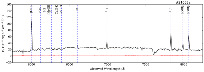
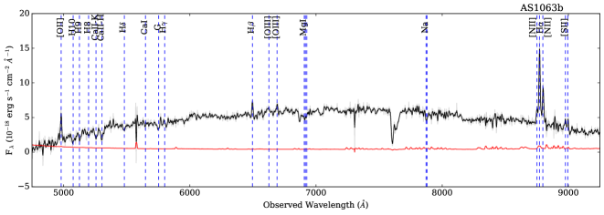
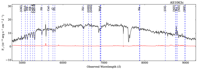
Figure 2: Magellan/LDSS-3 optical spectra of the three bright 24 $\micron$ sources in AS1063. (Top) Multiple Balmer lines (H$\alpha$ – H8) are detected in AS1063a suggesting it has undergone a recent burst of of star formation. (Middle and Bottom) We detect H$\alpha$ in the cluster members (AS1063b and AS1063c) suggesting that they may be falling into the cluster for the first time.

Table 1: Photometry of Three Bright 24 $\micron$ Sources

	AS1063a	AS1063b	AS1063c
Band	Magnitude	Magnitude	Magnitude
	[AB]	[AB]	[AB]
F225W	21.48$\pm$0.05	$<$22.88	$<$23.41
F275W	21.01$\pm$0.03	22.46$\pm$0.15	22.24$\pm$0.08
F336W	20.96$\pm$0.05	22.33$\pm$0.11	21.90$\pm$0.05
F390W	20.94$\pm$0.07	21.83$\pm$0.04	21.67$\pm$0.04
F435W	20.68$\pm$0.06	21.57$\pm$0.16	21.37$\pm$0.06
F475W	20.55$\pm$0.08	21.47$\pm$0.12	20.85$\pm$0.07
F606W	19.81$\pm$0.04	20.50$\pm$0.04	19.86$\pm$0.03
F625W	19.58$\pm$0.06	20.28$\pm$0.06	19.62$\pm$0.04
F775W	19.10$\pm$0.04	19.86$\pm$0.05	19.22$\pm$0.03
F814W	19.01$\pm$0.05	19.68$\pm$0.06	19.13$\pm$0.04
F850LP	18.85$\pm$0.08	19.52$\pm$0.09	18.95$\pm$0.06
F105W	18.54$\pm$0.01	19.30$\pm$0.02	18.77$\pm$0.01
F110W	18.47$\pm$0.01	19.16$\pm$0.02	18.67$\pm$0.01
F125W	18.42$\pm$0.02	19.02$\pm$0.03	18.54$\pm$0.02
F140W	18.25$\pm$0.01	18.89$\pm$0.01	18.42$\pm$0.01
F160W	18.07$\pm$0.02	18.75$\pm$0.02	18.31$\pm$0.02
Band	Flux	Flux	Flux
	[mJy]	[mJy]	[mJy]
3.6 $\mu$m	0.35$\pm$0.03	0.13$\pm$0.01	0.18$\pm$0.02
4.5 $\mu$m	0.29$\pm$0.03	0.12$\pm$0.01	0.17$\pm$0.02
5.8 $\mu$m	0.37$\pm$0.04	0.09$\pm$0.01	0.10$\pm$0.01
8.0 $\mu$m	0.30$\pm$0.04	0.22$\pm$0.02	0.12$\pm$0.01
24 $\mu$m	2.22$\pm$0.02	0.77$\pm$0.01	0.27$\pm$0.03
70 $\mu$m	32.2$\pm$2.3	9.0$\pm$0.5	$<$3.1
100 $\mu$m	69.3$\pm$4.9	14.5$\pm$1.0	3.7$\pm$0.8
160 $\mu$m	105.8$\pm$7.5	24.8$\pm$1.3	$<$8.2
250 $\mu$m	69.3$\pm$6.8	11.9$\pm$5.4	$<$16.2
350 $\mu$m	36.1$\pm$6.2	$<$17.1	$<$17.1
500 $\mu$m	21.9$\pm$6.1	$<$17.5	$<$17.5

Note. — Herschel errors listed are computed from the RMS of the maps plus the calibration error, which is 5% in PACS and 4% in SPIRE. PACS and SPIRE flux limits were presented in Rawle et al. (2016).

Our follow-up optical spectroscopy showed that the brightest 24 $\mu$m source (AS1063a) corresponds to a background galaxy at $z=0.61$, detecting Balmer emission (H$\beta$-H8), [O II]$\lambda$3727, [O III] $\lambda\lambda$4959,5007, and [Ne III]). The other two fainter 24 $\mu$m sources (AS1063b and AS1063c) correspond to cluster galaxies at $z=0.347$, detecting Ca ii H and K absorption and H$\alpha$ and [N II] $\lambda\lambda$ 6548,6583. The three 24 $\micron$ sources are listed in Table 4 and their optical spectra are plotted in Figure 2). These redshifts are consistent with those published by Gómez et al. (2012).

The MMIRS near-infrared spectrum of AS1063a detect H$\alpha$ and [N II]$\lambda$6585 lines (Figure 3) and the HST WFC3/IR G102 grism spectrum detect H$\alpha$ blended with [N II]$\lambda\lambda$6548,6583 lines (Figure 4). In addition, the grism also detects [S II]$\lambda$6717,6731 and [S III]$\lambda$9069,9545. The measured line fluxes are shown in Table 2 and 3. The line fluxes corrected for slit loss are also given, as described in Sections 2.4 and 2.5. The HST WFC3/IR G102 grism observations of H$\alpha$+[N II] is consistent with the Magellan/MMIRS measurement of those lines.

Table 2: Optical and Near-Infrared Emission Line Fluxes of AS1063a

Line	Flux	Fluxcorra
	($10^{-17}{\rm erg/s/cm}^{2}$)	($10^{-17}{\rm erg/s/cm}^{2}$)
Entire galaxy
[O II]$\lambda$3727	123.8$\pm$1.5	132.1$\pm$1.6
H$\delta$	10.3$\pm$0.8	11.0$\pm$0.9
H$\gamma$	25.9$\pm$1.1	27.7$\pm$1.2
H$\beta$	74.4$\pm$2.0	80.0$\pm$2.1
[O III]$\lambda$4959	33.0$\pm$2.8	35.3$\pm$3.1
[O III]$\lambda$5007	67.4$\pm$1.7	72.0$\pm$1.8
H$\alpha$	308.1$\pm$8.2	348.8$\pm$9.3
[N II]$\lambda$6583	137.7$\pm$6.9	155.9$\pm$7.8
H ii region
[O II]$\lambda$3727	61.6$\pm$0.8	65.8$\pm$0.9
[Ne III]$\lambda$3869	2.9$\pm$0.6	3.1$\pm$0.6
H8	4.2$\pm$0.5	4.5$\pm$0.5
H$\epsilon$	2.8$\pm$0.4	3.0$\pm$0.4
H$\delta$	7.0$\pm$0.4	7.5$\pm$0.4
H$\gamma$	17.1$\pm$0.5	18.4$\pm$0.5
H$\beta$	42.3$\pm$0.7	45.5$\pm$0.8
[O III]$\lambda$4959	15.5$\pm$0.7	16.7$\pm$0.8
[O III]$\lambda$5007	48.3$\pm$0.6	51.9$\pm$0.6
Bulge
[O II]$\lambda$3727	40.2$\pm$0.9	43.0$\pm$1.0
H$\delta$	2.9$\pm$0.4	3.1$\pm$0.4
H$\gamma$	8.4$\pm$0.7	9.0$\pm$0.7
H$\beta$	25.5$\pm$1.1	27.3$\pm$1.2
[O III]$\lambda$4959	7.4$\pm$1.4	7.9$\pm$1.5
[O III]$\lambda$5007	14.1$\pm$0.8	15.1$\pm$0.9
Spiral arm
[O II]$\lambda$3727	9.1$\pm$0.5	9.7$\pm$0.5
H$\gamma$	1.3$\pm$0.3	1.4$\pm$0.3
H$\beta$	2.4$\pm$0.6	2.6$\pm$0.6
[O III]$\lambda$5007	2.4$\pm$0.3	2.6$\pm$0.3

Note. — ^(a) Flux corrected for slitloss by convolving the HST ACS and WFC/IR images by the LDSS-3 and MMIRS seeing and measuring the ammount of light that is blocked by the slit.

Table 3: HST/WFC3 G102 and G141 Spectra of AS1063a

Line	Flux
	($10^{-17}{\rm erg/s/cm}^{2}$)
Entire galaxy
H$\alpha$+[N II]$\lambda\lambda$6548,6583	545.5$\pm$2.4
H ii region
[O III]$\lambda$5007	53.2$\pm$4.1
H$\alpha$+[N II]$\lambda\lambda$6548,6583	275.0$\pm$1.2
[S II]$\lambda\lambda$6717,6731	15.1$\pm$0.6
[S III]$\lambda$9069	4.4$\pm$0.6
[S III]$\lambda$9545	32.5$\pm$0.7
Bulge
H$\alpha$+[N II]$\lambda\lambda$6548,6583	205.1$\pm$1.5
Spiral arm
H$\alpha$+[N II]$\lambda\lambda$6548,6583	50.5$\pm$1.2

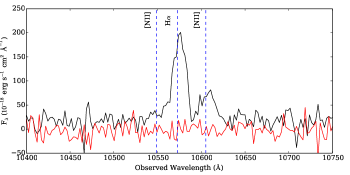
Figure 3: Magellan/MMIRS spectrum of AS1063a, H$\alpha$ and [N II]$\lambda$6585 are clearly detected within 20 minutes of integration. The asymmetry of the line is the result of the velocity offset of the bright clump at the edge of the galaxy. Even though the magnification is increasing across the galaxy towards the clump (southeast direction), it is not a major contributor to the asymmetry.

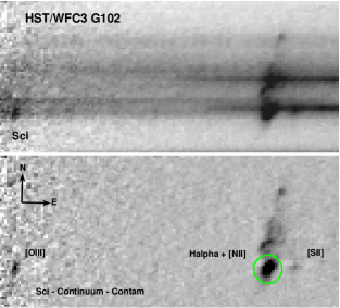
Figure 4: HST WFC3/IR G102 spectrum of the lensed galaxy AS1063a. (top panel) The reduced aXe spectrum. (bottom panel) The green circle marks the position of the star forming region. The reduced aXe spectrum with the contaminating sources subtracted and AS1063a continuum subtracted, using a sliding median. H$\alpha$+[N II]$\lambda\lambda$6548,6583 are detected throughout the entire galaxy, while [O III]$\lambda$5007 and [S II]$\lambda\lambda$6717,6731 are only detected for the star forming region.

AS1063a is detected in all three PACS bands (Figure 1). At 70 and 100 $\micron$ it is distinctly identifiable whereas at 160 $\micron$ it becomes blended with AS1063b. The third bright source (AS1063c) is detected at 70 $\micron$ and marginally detected at 100 and 160 $\micron$. The sources were not severely crowded and it was possible to get similar photometric values ($<7\%$ difference) doing both aperture and point spread function (PSF) photometry. Aperture photometry was used at 70 and 100 $\micron$ and PSF photometry was used at 160 $\micron$.

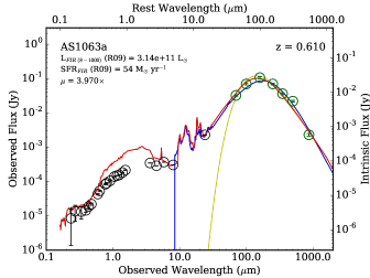
Figure 5: SED of the lensed galaxy AS1063a in the core of AS1063. Fits were made to the Herschel PACS 70, 100, 160 $\micron$ and Herschel SPIRE 250, 350, 500 and LABOCA 870 $\micron$ (green circles). The photometry blueward of the 70 $\micron$ was ignored in the fitting of the SED (black circles). The lines shows the best fitting templates to the far-IR/submm data. The blue line is the Rieke et al. (2009) templates and the red line is the Chary & Elbaz (2001) templates. The yellow line shows the best fitting modified blackbody. On the right axis, the observed flux was corrected based on the magnification (4.0$\pm$0.1) determined by the lens modelling by lenstool (Jullo et al., 2007).

At 250 $\micron$ AS1063a was blended with the nearby cluster galaxy AS1063b, and crowded field photometry (PSF fitting) was necessary to properly deblend the sources. The SED for AS1063a is shown in Figure  5. Within the cluster field it was difficult to find bright well-isolated sources to measure the PSF of the image, so we used an empirical PSF provided by the Herschel Science Center. The empirical PSF was binned and rotated to the PA of Herschel when it observed AS1063 and after subtracting the sources from the map had a resulting RMS of $\sim$5.9 mJy. At longer wavelengths (350 and 500 $\micron$) the two cluster members are almost completely undetected.

In order to determine the optical/near-IR counterpart of a submillimeter source it is necessary to have several bands spanning a wide wavelength range between the optical and the submillimeter. Sources are traced from the submillimeter to the optical, stepping down in wavelength while ensuring that each source is being followed near the centroid of the original submillimeter source. Sometimes submillimeter sources may be blends of multiple IRAC and MIPS sources. If the sources are not too close (less than a pixel away), then they can be deblended using the iraf task daophot with the IRAC and MIPS position priors. The redshift of the sources can also alleviate source confusion, where dust emission from lower redshift sources may fall below the detection limit for longer wavelength SPIRE bands.

Table 4: Spectroscopic Redshifts of Three Bright 24 $\micron$ Sources

Source	R.A.	Decl.	z${}^{\tablenotemark{a}}$	z${}^{\tablenotemark{b}}_{\rm quality}$	ID${}^{\tablenotemark{c}}$
AS1063a	22:48:41.760	-44:31:56.53	0.611	4	30
AS1063b	22:48:42.113	-44:32:07.39	0.337	4	8
AS1063c	22:48:42.480	-44:32:12.99	0.337	4	9

A complete list of 24 $\mu$m sources with spectroscopic redshifts within the deepest MIPS coverage of AS1063 (5′$\times$5′) is presented in Appendix A. A full analysis will be presented in a future paper.

3.2 IR-Luminous Lensed Galaxy at $z=0.61$

In the infrared/submillimeter range, the most conspicuous source in the core of AS1063 is the infrared-bright galaxy at $z=0.61$ (Figure 1). Its SED was fit using Chary & Elbaz (2001) and Rieke et al. (2009) templates (Figure 5). Both template sets are based on SEDs of local galaxies. The best $\chi^{2}$ model produces a total infrared luminosity, integrated from 8-1000 $\micron$ (Kennicutt, 1998), of $1.3\times 10^{12}\ \rm L_{\sun}$ $\mu^{-1}$, where $\mu$ is the magnification factor. The dust temperature was determined to be 36$\pm$1 K by fitting a modified blackbody to the peak of the dust bump with $\beta$ fixed at 1.5, using Eq. 1.

$$S_{\nu}=N(\nu/\nu_{0})^{\beta}B_{\nu}(T)$$ (1)

B_ν is a Planck function (evaluated at single temperature T), N is the amplitude, $\nu$ is the frequency, $\nu_{0}$ is the frequency which is typically fixed at c/250 $\micron$, and $\beta$ is the exponent that determines the shape of the modified blackbody.

The Spitzer/IRS spectrum of this galaxy is shown in Figure 6, and the measured line fluxes are listed in Table 5. The rest-frame mid-infrared spectrum looks like that of a star-forming galaxy, with a strong PAH feature (11.3 $\mu$m). The measured [Ne III](15.5 $\mu$m)/[Ne II](12.8 $\mu$m) line ratio is less than 1 (0.33$\pm$0.06), a value typical of a solar-metallicity starburst galaxy (Thornley et al., 2000; Rigby & Rieke, 2004). It is therefore clear that the predominant source of the infrared-luminosity is star-formation and not an AGN. This is consistent with the fact that the measured optical line ratios put this galaxy on the edge of the star forming sequence/composite region in the BPT diagram (Figure 7)

Table 5: Mid-IR Line Fluxes of AS1063a

Line	Wavelength	Flux
	($\mu$m)	($10^{-17}{\rm erg/s/cm}^{2}$)
[Ar III]	9.0	7$\pm$15
H2 S(3)	9.7	47$\pm$11
[S IV]	10.5	62$\pm$13
H2 S(2)	12.2	38$\pm$15
[Ne II]	12.8	238$\pm$16
[Ne III]	15.5	78$\pm$13
H2 S(1)	17.0	32$\pm$13
[S III] 18	18.7	167$\pm$ 8

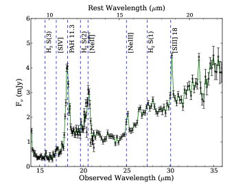
Figure 6: The Spitzer/IRS spectrum of the lensed galaxy AS1063a. We observe the [Ne iii] and [Ne ii] lines which we use to determine if our galaxy is undergoing AGN.

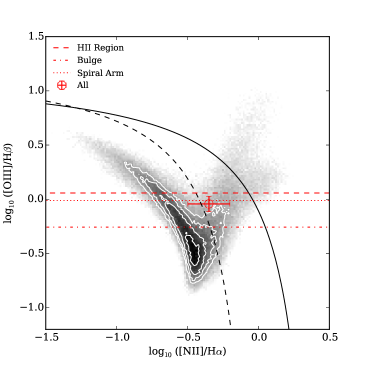
Figure 7: The BPT diagram of the three regions within the lensed galaxy AS1063a. The grayscale points are a 2D histogram of SDSS measured line ratios of redshifts between z = 0.005 - 0.25. The red lines mark the [O iii]/H$\beta$ ratios of three regions of the galaxy constrained by the optical data. Follow-up NIR observations in poor seeing conditions roughly constrain the [N ii]/H$\alpha$ ratio of the entire galaxy. The black lines mark the Kewley et al. (2001) and Kauffmann et al. (2003) predictions for active galaxy type. The error bars include a 20% systematic error in the flux calibration.

The HST images show that this galaxy has a spiral-like morphology with clearly defined bulge and disk components (Figure 8). In our optical spectrum obtained along the long axis of the galaxy shows a velocity offset from one side to the other (Figure 9), caused by the rotation of the disk component. The proximity of the $z=0.61$ galaxy to the cluster center suggests that its gravitational magnification is likely significant although its normal-looking morphology of a spiral galaxy indicates that the magnification effect is not large enough to destroy the intrinsic galaxy morphology, essentially stretching the galaxy in the direction tangential to the cluster center.

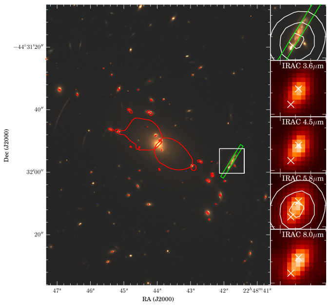
Figure 8: (left panel) Three color image of the cluster core AS1063 using HST ACS F606W, and HST WFC3/IR F110W and F160W filters. The main panel shows the central 1.0′$\times$1.2′ area of the cluster core. The red line marks the critical line at $z=0.61$. The green box marks the position of the slit used for optical spectroscopy of lensed galaxy AS1063a. The white box in the left panel shows the FOV of the source AS1063a displayed in the right panels. (right panels) The top right panel shows the zoomed HST three color image, using the same filters at the left panel. The bottom four panels show each of the Spitzer/IRAC 3.6, 4.5, 5.8 and 8.0 $\micron$ images with the same FOV as the top right panel. The white contour marks the position of the MIPS 24 $\micron$ contour. White x’s mark the positions of the bright star forming region and bulge.

Figure 1 clearly shows that the brightest infrared/submillimeter emission comes from this lensed galaxy at $z=0.61$. It is, however, not clear which part of the galaxy is exactly responsible for this strong infrared emission. Figure 8 shows that the peak of the brightest 24 $\mu$m emission is located 1.27″ SSE from the galaxy nucleus, falling in the middle of the disk. No bright optical/near-IR counterpart is seen at the peak of the 24 $\micron$ emission although three smaller star forming clumps are seen nearby in the HST images. The 24 $\micron$ emission appears resolved in one axis, elongated along the longer axis of the galaxy, suggesting the possibility that the 24 $\micron$ emission may originate from multiple components in the galaxy.

3.2.1 Bright Optical Clump with Strong Line Emission

What is most striking about the $z=0.61$ lensed galaxy, which corresponds to the brightest MIPS 24 $\mu$m and PACS/SPIRE source, is its exceptionally bright optical clump seen at one edge of the disk, 2.48″ southeast from the center of the galaxy. The CLASH HST data show that this clump is the brightest feature in all of the HST/ACS optical bands. In the HST/WFC3 near-infrared bands, however, the central bulge becomes the dominant feature.

This bright optical clump appears to have a quite significant size intrinsically. By fitting an elliptical Gaussian to the HST WFC3/IR F105W image (which corresponds to rest-frame H$\alpha$) and subtracting in quadrature a Gaussian point spread function (PSF) measured in the same image, we have derived the spatial size of this clump as 0.547$\pm$0.025″$\times$ 0.099$\pm$0.034″. This corresponds to 3686$\pm$171 pc $\times$ 670$\pm$230 pc at $z=0.61$ if we do not take into account the lensing effect.

The 2D spectra of the $z=0.61$ galaxy shown in Figures  4 and 9 show that the bright clump emits strongly in line emission (e.g., Balmer lines H$\alpha$ - H8, forbidden lines [O II] $\lambda$3727, [O III] $\lambda\lambda$4959,5007, [Ne III], [S II] and [S III]). Although we do detect the line emission throughout the galaxy disk, it quickly becomes fainter away from the clump while the Ca ii H and K absorption features become more prominent, reflecting an increasing light contribution from an older stellar population in the bulge and spiral arm area on the other side of the galaxy (Figure 9).

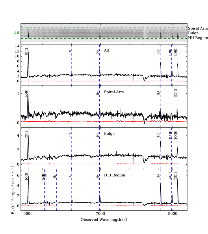
Figure 9: (first panel) The 2D spectrum of the lensed galaxy AS1063a taken with Magellan’s LDSS-3. (second panel) The 1D spectrum of the entire galaxy. (third panel) The 1D spectrum of the spiral arm. There appears to be an older stellar population, the Balmer lines are the weakest in this part of the galaxy. (fourth panel) The 1D spectrum of the bulge . This region corresponds to the central region of the 2D spectrum and the central region of the lensed galaxy. This region appears to have a significant older stellar population. (fifth panel) The 1D spectrum of the H ii region. This region corresponds to the lower bright part of the 2D spectrum. This is the bright star forming clump that is dominated by strong Balmer and forbidden emission lines.

4 Discussion

4.1 Lens Model Reconstruction

In order to determine the intrinsic properties of AS1063a it was necessary to remove the effects of gravitational lensing. Modelling of the gravitational lens, in the strong regime, was done with lenstool (Kneib et al., 1996; Jullo et al., 2007; Jullo & Kneib, 2009). lenstool models the cluster lenses by utilizing a non-parametric method, using multiple images and redshifts of lensed background galaxies in order to constrain the model. In the newest CLASH data, we identified 5 multiply imaged systems, one of which was confirmed with a spectroscopic redshift, that were used as input constraints for the lens model (Richard et al., 2014, Clément et al. in prep). With the lens model it was possible to determine critical lines and spatial and flux magnifications of the lensed galaxy.

From the lens model we are able to reconstruct AS1063a in the source plane (Figure 10, right panel). Most of the magnification is linear, with very little distortion.

The luminosity-weighted magnification is 4.0$\pm$0.1. The error in the magnification is the statistical error and does not include systematics such as choice in parameterization/modelling or use of bad constraints/assumptions in the model. AS1063a is $\sim$5″ from the critical line which suggests that is too far for differential magnification to be a significant factor.

There is a slight gradient in the spatial distortion of the galaxy, from the southern edge to the northern edge, 3.6$\times$ - 2.6$\times$ in linear magnification. In ACS this resolves objects larger than 90 - 130 pc, and WFC3/IR 240 – 340 pc. The LDSS-3 spectrum, at 0.76″ seeing, spatially resolves 1.4 - 2.0 kpc. The flux amplification from the southern edge to the northern edge is 4.5$\times$ - 3.1$\times$, as shown in the right panel in Figure 10. The bright star forming clump corresponds to the region of the larger amplification at the southern edge of the galaxy.

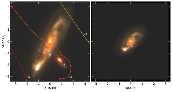
Figure 10: (left) HST three color image (ACS F606W and F814W, and WFC3/IR F110W filters) of the lensed galaxy AS1063a. The contours represent the flux amplification map of the AS1063 lens. (right) The source plane reconstruction performed by lenstool. Most of the magnification is linear along the major axis of the galaxy. The morphology of the lensed galaxy clearly is a spiral galaxy with two prominent spiral arms. The bright star forming clump is the dominant feature in all ACS/WFC3 bands.

The bulge of AS1063a is prominent in the F775W filter and longward wavelengths. When comparing the observed image to the reconstructed image, the galaxy only appears stretched in the observed image (Figure 10, left). From the reconstructed image a few noticeable features pop out; there are two spiral arms, a bulge and multiple bright clumps (star forming knots) with one very prominent bright clump (the giant H ii region). The magnification at the giant bright clump is 4.44$\times$.

We discovered that there is also disagreement with the lens model constructed by Gómez et al. (2012). A redshift was obtained for “Lens B” and “Lens C” as designated by Gómez et al. (2012), which is one of the main constraints for the non parametric lens model. According to our lens model, based on the location of the bright arc, AS1063a or “Lens A”, it is well outside the $z=0.61$ critical line and no additional images are expected for this arc. The suggested counter image to “Lens A”, “Counterpart A” is another lensed arc. With the additional resolution provided by the CLASH data, it is clear that the colors do not match the colors of the bright arc, and the bright clump seen in the “Counterpart A” is not the bright clump identified in the bright arc, but highly suggestive of a cluster galaxy.

4.2 Physical Properties of the $z=0.61$ Lensed IR-Luminous Galaxy

4.2.1 Star Formation Rates

When corrected for a magnification factor of 4.0$\pm$0.1, the intrinsic infrared luminosity of the $z=0.61$ galaxy becomes (3.1$\pm$0.1) $\times 10^{11}\ \rm L_{\sun}$ with a corresponding star formation rate of 54$\pm$2 M_☉ yr^-1. This means that this galaxy is intrinsically infrared-luminous and of the LIRG type (Luminous Infrared Galaxy, L${}_{\rm IR}\geq 10^{11}\ \rm L_{\sun}$.)

On the other hand, the star formation rate (SFR) derived from H$\alpha$, detected with MMIRS, is significantly smaller. The observed H$\alpha$ line luminosity gives a star formation rate of 28$\pm$1 M_☉ yr^-1. Corrected for magnification, the value decreases to 7.0$\pm$0.3 M_☉ yr^-1. When corrected for a visual extinction of A${}_{\rm V}=$ 1.5$\pm$0.2 mag (E(B-V) = 0.36$\pm$0.04) derived from the Balmer decrement assuming case B recombination and using a Calzetti dust law, the value increases to 33$\pm$1 M_☉ yr^-1, but this is still smaller than the infrared-derived value of 54$\pm$2 M_☉ yr^-1. This implies that 40% of the star formation is obscured.

The HST grism spectrum of AS1063a is at a spatial resolution of 0.13″. At this spatial resolution we can determine the contributions for the spatially distinct components of the galaxy (i.e. H II region, bulge and spiral arm). In order to utilize this information, we need to assume an [N II]/H$\alpha$ ratio. From the MMIRS spectrum for the entire galaxy, we measure a ratio of 0.45$\pm$0.03, which we assume for each of the regions in the galaxy. Unfortunately, the seeing and S/N of the MMIRS spectrum is not sufficient enough to determine the ratio for the spatially distinct components of the galaxy. We also assume that the ratio between [N II]$\lambda$6583/[N II]$\lambda$6548 $\sim$ 3. With this we estimate the H$\alpha$ flux for the entire galaxy as $340.9\pm 26.3\times 10^{-17}$ ergs s^-1 cm^-2; 171.9$\pm$13.3 ergs s^-1 cm^-2 for the H II region, 128.2$\pm$9.9 ergs s^-1 cm^-2 for the bulge and 31.6$\pm$2.5 ergs s^-1 cm^-2 for the spiral arm. Using the E(B-V) computed for the entire galaxy and correcting for the magnification of each of the regions (i.e. 4.4$\times$, 3.9$\times$, and 3.3$\times$), we find that the SFR for each of the regions are the following: 14$\pm$1 M_☉ yr^-1 for the H II region, 12$\pm$1 M_☉ yr^-1 for the bulge, and 4$\pm$1 M_☉ yr^-1 for the spiral arm.

In §4.2.3, E(B-V) is also computed from the SED fitting of the photometry for AS1063a and its H II region, which are 0.31 and 0.18 respectively. If we assume these E(B-V) values and magnification corrections, it would affect the HST grism based SFRs in the following way: 27$\pm$2 M_☉ yr^-1 for AS1063a and 8$\pm$1 M_☉ yr^-1 for the H II region. The overall E(B-V) computed for the galaxy from the Balmer decrement agrees with the one computed from the photometry. However, for the H II region, it might be expected that there could be some geometry or sight-line effect that could result in a different E(B-V) value. In particular, lower in this case, which is evident by the H II region being the brightest feature in the galaxy in the UV-optical bands as well as detecting more Balmer transitions (i.e. H$\alpha$-H8). For the H II region we adopt the SFR = 8$\pm$1 M_☉ yr^-1 that is derived using the E(B-V) value from the photometry, which seems more consistent with the evidence.

Using H$\beta$ and H$\gamma$ and H$\delta$ lines seen in the 2D optical spectrum (Figure 9), we can derive visual extinctions and extinction-corrected star formation rates for spatially distinct components in the galaxy. However, the E(B-V) values disagree with the one derived from H$\alpha$ and H$\beta$, increasing with higher order Balmer transitions. Upon further inspection it appears that self absorption from the continuum could be affecting the flux measured for the higher order Balmer lines.

4.2.2 Precise Location of the Infrared Source

As we mentioned in §3.2 the MIPS 24 $\micron$ emission is offset from the bulge of the $z=0.61$ galaxy by 1.27″and elongated, suggesting it is resolved in one axis. One concern is whether the offset is real or if it is a result of astrometric error due to the large MIPS 24 $\micron$ PSF. The native pixel scale of the MIPS 24 $\micron$ is 2.45″ pixel^-1. However, the image we use is sampled at 1.245″ pixel^-1. In order to compare the bulge position to the MIPS position we need a set of unresolved sources that can be used for astrometry. For the $z=0.61$ lensed galaxy, the bulge can be identified in the F814W filter, which is also convenient due to the larger FOV of ACS. We used two methods to identify stars in the HST F814W images; 1) plotting the difference in the magnitude of two different sized apertures and 2) plotting magnitude versus half-light radius at a fixed aperture. Stars will resemble the PSF of the instrument for a wide range of radii, whereas if just using a FWHM measure, some galaxies may have similar FWHM as a star and lead to a false positive detection. As an additional check, we visually inspected stars to ensure sources were not misidentified and were not blended with other sources. For sources we believe to be stars, we checked to see whether they are detected in IRAC and also to ensure they are not blended. From our clean list of point sources, we compute the separation angle between the sources detected in ACS and IRAC. We then measure the standard deviation of all the separations, computing the 1$\sigma$ error in the astrometric position of 0.12″.

At 24 $\micron$ many of the sources are unresolved, very few of which are actually stars. In order to determine the astrometric error between IRAC and MIPS we rely on compact sources that are unresolved in IRAC. We use a similar strategy to the one described above to select point sources in IRAC. We compute the standard deviation of the separation angle between the positions in IRAC to the positions in MIPS and find an error of 0.23″. The combined 1$\sigma$ error in the astrometric positions in ACS, IRAC and MIPS is 0.26″. At 4.9$\sigma$ we can confidently say that the offset of the MIPS peak emission is real.

In order to explain the elongation of the source in MIPS 24 $\micron$, we simulate the source by convolving a Gaussian with the MIPS PSF. We then assume the position is at the center of the peak MIPS emission and vary the amplitude while minimizing $\chi^{2}$. We find that a single source at the peak of the 24 $\micron$ emission is not sufficient to account for all the flux in the source, which has significant residual wings. To account for all the flux it appears that more than one Gaussian is needed. We next assume that the far-IR emission could be coming from two locations, offset from the peak emission. Two reasonable locations are the bulge of the galaxy and the star forming region. We find that fitting two Gaussians at those locations works well. The residuals are much smaller with the majority of the flux being accounted for. The solution that works the best is two Gaussians with roughly the same amplitude. However, these solutions are highly degenerate and additional Gaussians could potentially be added for better fits. We can confidently say that it is unlikely that a single source is responsible for all of the far-IR emission at the position of the 24 $\micron$ emission peak. There must be more than one source contributing to the far-IR flux; higher spatial resolution is needed to resolve the situation.

Looking at the IRAC bands, there is a slight bump at 5.8 $\micron$. Based on the redshift of this galaxy, it is expected that the 3.3 $\micron$ PAH feature would be completely in the band. However, the 3.3 $\micron$ PAH feature is much weaker than the other PAH features found in star forming galaxies and the bump we see in the SED may not be caused by this feature. It is expected that the majority of light contributing to the flux in the IRAC bands is from stars. If there is flux coming from the 3.3 $\micron$ PAH feature, we would need to subtract off the stellar light. To account for the stellar light, we scale the flux in IRAC 3.6 to the IRAC 5.8 $\micron$ image and subtract them from each other. We also do the same with the IRAC 4.5 $\micron$ image. In each case there appears to be no evidence for residual flux coming from the 3.3 $\micron$ PAH feature. If the bump seen in the SED is real, it is possible that the PAH emission could be throughout the galaxy at a low enough level that it might not be seen in the residuals. It appears unlikely that the flux would be originating from an individual region in the galaxy, otherwise it should have been seen in the residuals.

4.2.3 Stellar Mass

Table 6: Stellar Mass of AS1063a

Metallicity	Av	Age	Stellar mass
[$Z_{\sun}$]		[Gyr]	[$M_{\sun}$]
Entire galaxy
1.000	1.25${}^{+0.21}_{-0.48}$	0.65${}^{+0.48}_{-0.27}$	2.6${}^{+1.5}_{-1.0}\times 10^{10}$
0.005	1.61${}^{+0.18}_{-0.19}$	0.64${}^{+0.53}_{-0.21}$	3.0${}^{+1.7}_{-1.1}\times 10^{10}$
H ii region
1.000	0.74${}^{+0.20}_{-0.24}$	0.38${}^{+0.31}_{-0.17}$	10.5${}^{+6.1}_{-3.9}\times 10^{8}$
0.200	1.15${}^{+0.30}_{-0.41}$	0.10${}^{+0.16}_{-0.07}$	7.1${}^{+4.1}_{-2.6}\times 10^{8}$

We fit the HST 16-band photometry to Bruzual & Charlot (2003) models following Pérez-González et al. (2008, 2013) in order to determine stellar mass, dust attenuation, and stellar age and population. We assume a Chabrier IMF, Calzetti extinction and exponentially decreasing star formation history. The models were run fixing the metallicity to solar metallicity and also allowing it to be a free parameter. The SED fitting was conducted on the photometry of AS1063a and just the H ii region. The images used for the photometry of the H ii region were PSF matched to ensure that we are comparing the same physical region in each band. We used TinyTim (Krist et al., 2011) to generate the PSF for each of the 16 bands, convolved with the charge diffusion PSF and rebinned to the CLASH pixel scale of 65 mas. The iraf task psfmatch was used to convolve all of the HST images to the WFC3/F160W PSF.

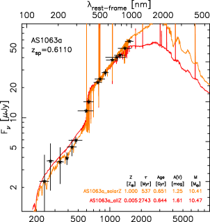
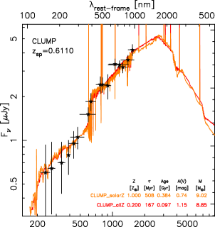
Figure 11: Left: SED fits to the intrinsic flux of the entire galaxy, AS1063a. Right: SED fits to the intrinsic flux of H II region in AS1063a. The templates used assume a Chabrier IMF, Calzetti extinction and exponentially decreasing star formation history. The orange line shows solar metallicity template and the red line is the best fitting metallicity. From the photometry fitting, for both AS1063a and the clump, neither model is preferred. The metallicity determined from the nebular emission lines from the R23 and N2 diagnostics help constrain which model is the appropriate one, that being the solar metallicity model.

The results of the SED fitting can be found in Table 6 and Figure 11. The stellar masses derived from the SED fitting are good to within 0.2 dex, including uncertainties in the IMF and other systematics. AS1063a’s stellar mass appears to be unaffected by metallicity as its mass varies by 1.1$\times$ for the metallicities considered. In §4.2.5 we describe the metallicity derived from the nebular emission lines in which we find the value is about solar metallicity. For AS1063a we adopt the stellar mass (2.6$\times 10^{10}\ \rm M_{\sun}$) at solar metallicity. The H II region on the other hand is seems to vary by a factor of 1.5$\times$ depending on the metallicity. We also adopt the solar metallicity value (1.1$\times 10^{9}\ \rm M_{\sun}$), in which it appears to be close to solar metallicity, as we go over in §4.2.5.

When comparing the H ii region in AS1063a to ones at higher redshift we find that is about average stellar mass, the high redshift H ii regions span $10^{7}$ – $10^{10}\ \rm M_{\sun}$. Looking at the samples individually; the H II regions in RCSGA0327 (Wuyts et al., 2014), a galaxy a $z=1.7$, fall on the lower mass side from $10^{7}$ – $10^{8}\ \rm M_{\sun}$ whereas the Wisnioski et al. (2012) and (Förster Schreiber et al., 2011b) samples are on the higher mass range $10^{9}$ – $10^{10}\ \rm M_{\sun}$ and $10^{8}$ – $10^{10}\ \rm M_{\sun}$. This can be mostly explained by Wisnioski et al. (2012) and Förster Schreiber et al. (2011b) samples being unlensed, so only the largest most massive H ii regions are probed, whereas the Wuyts et al. (2014) sample is a single lensed galaxy probing small H ii regions at high spatial resolution.

Using the stellar mass at solar metallicity for AS1063a and the SFR derived from the far-IR, we compute the specific star formation rate (sSFR), which is 2.11 Gyr^-1. We use the analytic fitting function from Whitaker et al. (2012) to determine the sSFR of the star-forming main sequence, which is 0.35 Gyr^-1 for a galaxy with the same stellar mass and redshift as AS1063a. Galaxies with sSFRs 4$\times$ the star-forming main sequence are considered starbursts (Rodighiero et al., 2011; Noeske et al., 2007). The starburst region for a galaxy similar to AS1063a is 1.38 Gyr^-1, which means that AS1063a is a starburst.

4.2.4 Kinematics

Spectroscopically, this bright clump appears like an H II region embedded in a rotating disk, with a rotational velocity V_max of 134$\pm$17 km s^-1 at $R=5.9$ kpc, which is also found by Gómez et al. (2012) and Karman et al. (2015). The clump itself shows strong Balmer emission (H$\alpha$ - H8), forbidden line emission ([O ii]$\lambda$3727, [O iii]$\lambda\lambda$4959,5007, [Ne iii]) emission, and its systemic velocity falls on the rotation curve. AS1063a has a smooth rotation curve that flattens out outside of 2 kpc (Figure 12).

Figure 12: (left) The kinematics of the observed [O II] emission line measured from the 2D spectrum. We measured the centroid of the blended [O II]$\lambda\lambda$3726,3729 doublet, which corresponds to [O II] $\lambda$3727. [O II] is the brightest feature spatially with the highest signal-to-noise ratio. In order to reduce the noise in the measurement, we binned the data into bins of 4 pixels each (0.76″), which is comparable to the seeing. (right) The intrinsic kinematics of the lensed galaxy AS1063a. The red line is the best fit velocity profile. The galaxy appears to have a slight inclination which is seen by a velocity gradient, suggesting that the galaxy is rotating as one system. The rotation curve appears to be flattening out outside 2 kpc.

A system in the local Universe with a similar appearance to AS1063a is NGC 5194 (M51), which is a spiral galaxy interacting with another galaxy (NGC 5195). Sofue et al. (1999) looked at the rotation curves of local galaxies and found that NGC 5194 had a peculiar rotation curve (non-Keplerian). NGC3034 (M82), a starburst galaxy interacting with M81, also shows a peculiar rotation curve, in which it has a steep Keplerian decline. In the local Universe it is expected that an isolated spiral galaxy should have a flat rotation curve at large radii (5-30 kpc). Significant bumps or deviations from Keplerian rotation in the rotation curve could indicate an interaction with another galaxy or underlying substructure (subhalos). Kinematically it is difficult to completely rule out AS1063a as a merger, however it appears unlikely.

From the rotation curve we can also measure a dynamical mass. In order to compute an accurate dynamical mass we need to determine the inclination of the galaxy. Using the source plane reconstruction of the galaxy, we measure the axis ratio (b/a) using galfit (Peng et al., 2002, 2010). We find an axis ratio of b/a = 0.502$\pm$0.007. Assuming the galaxy is an oblate spheroid (Holmberg, 1958), we use equation 2 to compute the inclination,

$${\rm cos}^{2}i=\frac{(b/a)^{2}-q^{2}}{1-q^{2}}$$ (2)

where $i$ is the inclination angle, $b/a$ is the axis ratio ($a$ is the semi-major axis, $b$ is the semi-minor axis of the galaxy), and $q$ is the axis ratio for an edge-on galaxy. Typically $q$ is 0.13 in spiral galaxies. In order to understand the uncertainty in the inclination angle we performed an MCMC using 1000 realizations of the AS1063 lens model (lenstool routine bayesCleanlens), with each realization reconstructing AS1063a and the HST PSF in the source plane. We then use galfit to fit each of the realizations of the reconstructed source plane image, using the reconstructed PSF associated with a reconstructed image. The standard deviation of the PA of the galaxy was 1.5^∘. Even with this deviation in the PA, we find that the uncertainty in the inclination is 0.5^∘. When we vary the parameter $q$, the disc thickness from 0.11–0.2 (Courteau, 1997), which is typical for spiral galaxies, we find the that it varies by 1.5^∘. Given the systematic uncertainties for determining inclinations of galaxies (e.g. Barnes & Sellwood (2003)), we adopt $\pm$5^∘ uncertainties on the inclination. We compute an inclination $i=61\pm 5^{\circ}$. The dynamical mass is defined by Eq. 3,

$$M_{\rm dyn}=\frac{RV^{2}}{G}$$ (3)

where $V=V_{r}\ sin(i)$ ($V_{r}$ is the radial velocity, $i$ is the inclination) and $R$ is the radius. Förster Schreiber et al. (2009) uses the velocity at 10 kpc which is typically the surface brightness limit of their sample, to determine the dark matter contribution of their galaxies. Looking at the rotation curves of nearby galaxies (Sofue et al., 1999), many of the rotation curves flatten out well beyond 10 kpc, which means that the baryons contribute more to the inner 10 kpc than dark matter. For AS1063a, the rotation curve flattens out after 4-5 kpc and it is not unreasonable to extrapolate the velocity at 10 kpc. Courteau (1997) demonstrates that the arctangent function is a good fit to galaxy rotation curves in the local Universe in order to determine the circular velocity at a given radius, shown in Eq. 4,

$$V(R)=V_{0}+\frac{2}{\pi}V_{c}\ {\rm arctan}\frac{R}{R_{t}}$$ (4)

where $V_{0}$ is the velocity center of rotation (systemic velocity), $V_{c}$ is the asymptotic velocity, and $R_{t}$ is the scale radius where the rotation curve begins to flatten out. We fit the AS1063a velocity curve with the arctangent function. Figure 12 (right panel) shows the fit to the intrinsic radius. The large error bars and scatter seen in the points that are furthest from the center are due to the low S/N of the fit to the [O II] line. If you allow the [O II] line to be fit at larger radius, the error bar increases significantly, which once again reflects the S/N decreasing.

With the inclination and the circular velocity at 10 kpc, we compute a dynamical mass of (5$\pm$1)$\times 10^{10}$ M_☉. This dynamical mass is comparable to the average SINS (Förster Schreiber et al., 2009) galaxy, which spans $\sim$1–20 $\times 10^{10}$ M_☉ for redshifts $z=1.3-2.6$.

4.2.5 Metallicity

Table 7: Metallicity of AS1063a

	$12+log([{\rm O/H}])$	$12+log([{\rm O/H}])$
	R23	N2
Entire galaxy	8.95$\pm$0.02	8.80$\pm$0.03
H II region	8.96$\pm$0.02	$\cdots$
Bulge	8.99$\pm$0.02	$\cdots$
Spiral arm	8.74$\pm$0.10	$\cdots$

As mentioned in §3.2 we detect key emission lines with LDSS-3 and MMIRS for determining metallicity. We use both R23 ([O ii]$\lambda$3727, H$\beta$, and [O iii]$\lambda$5007) and [O iii]/[O ii], and N2 (H$\alpha$ and [N ii]$\lambda$6585) diagnostics to determine the metallicity of the lensed galaxy at $z=0.61$ and its individual regions. We were unable to detect the [O iii]$\lambda$4363 line, a low metallicity indicator, which implies that we should choose the upper branch for R23.

For the N2 measurement we follow the prescription of Pettini & Pagel (2004) using their cubic relation. For the R23 measurement, we follow the prescription of Kewley & Ellison (2008), specifically following the KK04 method. The results for the metallicities can be found in Table 7. All the values are roughly consistent with solar metallicity. There is some evidence of a metallicity gradient from the spiral arm to the bulge. The metallicity is constant from the bulge to the H ii region.

Metallicity gradients are seen in the Milky Way, where the gas-phase metallicity is lower at larger radii than at the bulge. These metallicity gradients are also seen in local galaxies, where the slope of the gradient is shallow. The gradient in metallicity suggests that the metallicity throughout the disk of a galaxy is evolving over time. At higher redshift, in $z\sim 2$ galaxies (Jones et al., 2010a; Yuan et al., 2011; Jones et al., 2013), there is evidence for steeper metallicity gradients. It is suggested that there is inside-out growth in these galaxies that may be responsible for creating the steep metallicity gradients. In AS1063a, the metallicity gradient is not as steep as seen in $z\sim 2$ galaxies, and appears more like galaxies in the local Universe, shown in Figure 13.

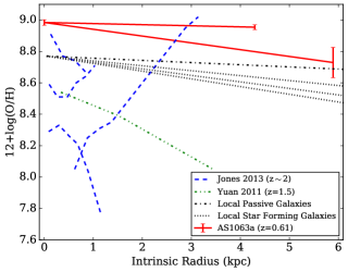
Figure 13: Metallicity as a function of radius for galaxies in the local Universe (Henry & Worthey, 1999; Rupke et al., 2010) and at high redshift gravitationally lensed sample (Yuan et al., 2011; Jones et al., 2013). The higher redshift galaxies show a steeper metallicity gradient than seen in the local Universe. AS1063a resembles more local star forming galaxy. We use the R23 to derive the metallcity in AS1063a. Jones et al. (2013) uses a variety of methods, we compare to their O3HB. (Yuan et al., 2011) uses N2.

There are known aperture effects when measuring metallicity, where low metallicity regions may be hidden by higher metallicity regions. While it appears that the metallicity is constant between the H ii region and the bulge of AS1063a, we may not be sensitive to the lower metallicity regions. This is primarily due to the spatial resolution of the spectra, determined by the seeing, and S/N of the fainter emission lines, such as the [O iii]$\lambda$4959.

The SINGS sample of H ii regions (Moustakas et al., 2010) in the local Universe spans metallicities 7.7 – 9.3 (KK04). The majority of H ii regions (88%) have metallicities between 8.6 – 9.2. The metallicity of the H ii region in AS1063a does not seem unusual when compared to the SINGS galaxies in the local Universe as 48% of their H ii regions have metallicities between 8.9 – 9.1. Higher redshift H ii regions seem to have lower metallicities when compared to the H ii region in AS1063a. Wisnioski et al. (2012) metallicities span 8.4 – 8.8, Jones et al. (2010a, 2013) span 8.2 – 9.0. and Wuyts et al. (2014) metallicities spans 8.0 – 8.3 for several H ii regions in RCSGA0327.

4.2.6 Gas Depletion Timescale

In order to estimate the molecular gas mass without a CO measurement there are two methods; (1) using the dust mass from the galaxy’s far-IR emission and (2) using the dynamical mass from the galaxy’s kinematics.

For the first method in determining gas mass, we need to measure the dust mass. To determine the dust mass from the far-IR emission, we use Eq. 5 (Greve et al., 2012),

$$M_{\rm dust}=\frac{D_{L}^{2}S_{\nu_{o}}}{(1+z)\kappa_{\nu_{r}}}[B_{\nu_{r}}(T_{\rm dust})-B_{\nu_{r}}(T_{\rm CMB}(z))]^{-1}$$ (5)

where $S_{\nu_{o}}$ is the observed flux, B${}_{\nu_{r}}$ is the rest-frame Planck function, $\kappa_{\nu_{r}}$ is the rest-frame absorption coefficient. The Planck function is defined at the dust temperature T_dust and the T_CMB at redshift z. The absorption coefficient is defined as $\kappa_{\nu_{r}}=0.45(\nu_{r}/250\ \rm GHz)^{\beta}$ (Hildebrand, 1983; Kruegel & Siebenmorgen, 1994), where $\nu_{r}$ is the rest-frame frequency and $\beta=2.0$. According to Papadopoulos et al. (2000) the temperature of the CMB affects the dust mass by $\sim$2%. da Cunha et al. (2013) also found that at redshifts $z<4$ the CMB temperature negligibly affects the dust mass and because of this we do not include it in our calculation. Using a T_dust = 36$\pm$1 K and using the LABOCA 870 $\micron$ flux we compute M_dust = (4.3$\pm$0.4) $\times 10^{7}\ \rm M_{\sun}$.

In order to compute the gas mass from the dust mass it is important to know the dust-to-gas ratio (DGR). Leroy et al. (2011); Sandstrom et al. (2013) shows that there is a correlation between metallicity and the DGR for local star forming galaxies and parameterized it using Eq. 6 for metallicities computed using KK04:

$${\rm log}({\rm DGR})=a+b(12+{\rm log}({\rm O/H})-c)$$ (6)

where a = -1.86, b = 0.85 and c = 8.39. Using the metallicity found for the entire galaxy from the R23 line ratio we find a DGR = 0.0114.

The relationship between molecular gas, H I and dust is shown in Eq. 7 (Leroy et al., 2011; Sandstrom et al., 2013)

$$\Sigma_{\rm D}/{\rm DGR}=\Sigma_{\rm HI}+\Sigma_{\rm H_{2}}$$ (7)

where $\Sigma_{\rm D}$ is the mas surface density of dust, $\Sigma_{\rm HI}$ is the mass surface density of H I, and $\Sigma_{\rm H_{2}}$ is the mass surface density of molecular gas. H I is difficult to detect at higher redshift (e.g. $z=0.4$ galaxy 180 hours VLA, Fernández et al., 2016) and because of this it is typically excluded from the total gas mass. However, LIRGs and ULIRGs (Ultra Luminous Infrared Galaxies, L${}_{\rm IR}\geq 10^{12}\ \rm L_{\sun}$) are observed in the local Universe to have more molecular gas than atomic (e.g. H₂/H I $>$ 1, Mirabel & Sanders, 1989), with the ratio of H₂/H I increasing with infrared luminosity. At most, the total molecular gas could be off by about 0.3 dex. More typically for submillimeter galaxies (SMGs) and ULIRGS the total H I mass is not significant (0.1 dex, Sanders & Mirabel, 1996; Santini et al., 2010). We find that the molecular gas mass is the following; $M_{\rm gas}=(3.8\pm 0.4)\times 10^{9}\ \rm M_{\sun}$.

With the gas mass and far-IR SFR ($54\pm 2\ \rm M_{\sun}\ \rm yr^{-1}$) we compute the gas depletion timescale of 70 Myr. If instead we assume a more conservative SFR, from the instantaneous SFR derived from H$\alpha$ (33$\pm$1 M${}_{\sun}\ \rm yr^{-1}$), it would suggest a depletion timescale of 120 Myr.

Comparing the gas mass to the stellar mass gives the gas fraction $f_{\rm gas}$ = 0.13${}^{+0.06}_{-0.04}$, defined as $f_{\rm gas}=M_{\rm gas}/(M_{\rm gas}+M_{\ast})$, or $M_{\rm gas}$ = (4.1$\pm$0.4)$\times 10^{9}\ M_{\sun}$. Comparing to other galaxies at this redshift (Daddi et al., 2010; Geach et al., 2011; Magdis et al., 2012), the gas fraction for this galaxy is typical and not unusual. The range of gas fractions at z$\sim$0.6 is about 0.05 – 0.3.

For the second method of determining the gas mass, we use the dynamical mass of the galaxy from §4.2.4. The gas mass is defined as $M_{\rm gas}=M_{\rm dyn}-M_{\ast}-M_{\rm dark}$, where the $M_{\rm dark}$ is the dark matter mass. If we assume a dark matter fraction of 0.2 – 0.3 within a radius of 10 kpc (Förster Schreiber et al., 2009) for galaxies $z=1-3$ we get a gas mass of $M_{\rm gas}$ = (7.7 – 12.4)$\times 10^{9}\ \rm M_{\sun}$, which is $f_{\rm gas}$ = 0.23 – 0.33, which is larger than what we compute using the dust mass. There are likely more uncertainties with the dynamical mass calculation, as the dynamical mass could be influenced by the position of the slit, not fully sampling the galaxy’s velocity field. In addition, inclination of the galaxy could also be large uncertainty, as the projection of the galaxy on the sky is highly degenerate, especially when considering diverse galaxy morphologies. Finally, the stellar mass could be underestimated, which could result in a larger gas fraction. From herein, we use the gas fraction based on the dust mass.

In §4.2.2 we find that as much as half of the far-IR flux could be associated with the H ii region (half of the SFR). Extending this to the molecular gas, if we assume that the molecular gas traces the dust, then roughly half of the molecular gas could be associated with the H ii region. This also suggests a similar depletion timescale of 70 Myr. Using the instantaneous SFR derived from H$\alpha$ from the HST grism ($8\ \rm M_{\sun}\ \rm yr^{-1}$) for the H ii region would suggest a depletion timescale of 230 Myr. Adding the depletion timescale to the stellar age (0.38${}^{+0.31}_{-0.17}$ Gyr) of the AS1063a H II region makes its lifetime 0.44 – 0.92 Gyr. However, even with a Balmer decrement, it is unclear if we are truly measuring the current instantaneous SFR or the dust attenuated one. In order to determine the lifetime of the H II region, even without instantaneous star formation tracers which are less affected by dust (i.e. P$\alpha$, P$\beta$), we rely on the far-IR SFR to set the maximum rate that stars form. We find that incorporating the range of SFRs and stellar ages provides a lifetime for the H II region being 0.28 - 0.92 Gyr. This is consistent with H II regions at $z\sim 2$ which are expected to live between 0.1 – 1 Gyr (Dekel et al., 2009; Genzel et al., 2011; Guo et al., 2012).

4.3 Giant ($\sim$kpc) H II Region Embedded in a Rotating Disk at $z=0.61$

Table 8: Physical Properties of AS1063a

Parameter	Value	Unit
T	36$\pm$1	K
LIR	(3.1$\pm$0.1)$\times 10^{11}$	L☉
SFR FIR	54$\pm$2	M☉/yr
SFR H$\alpha$	33$\pm$1	M☉/yr
Mdust	(4.6$\pm$0.4)$\times 10^{7}$	M☉
M∗	2.57${}^{+1.50}_{-0.95}\times 10^{10}$	M☉
Mdyn	(5$\pm$1)$\times 10^{10}$	M☉
Mgas	(4.1$\pm$0.4)$\times 10^{9}$	M☉
E(B-V)	0.36$\pm$0.04
AV	1.5$\pm$0.2	mag
fgas (Mdust)	0.13${}^{+0.06}_{-0.04}$
i	61$\pm$5	deg

Taking into account the effect of magnification, we divide by the linear magnification, determined by the lens model of the cluster, and find the FWHM of the clump in the source plane is 996$\pm$46 pc. In order to compute the error bar for the size of the H ii region we ran a Monte Carlo simulation, varying the noise and refitting the elliptical Gaussian for 1000 realizations, then measuring the standard deviation of the width measurements.

At the spatial resolution provided by the gravitational lensing, this means that the clump appears to be a single clump, with ACS resolving individual structures larger than 90 pc and WFC3/IR larger than 240 pc. While we can not completely rule out the possibility, it appears unlikely to have $>$10 smaller clumps lined up in a chain, appearing like a single 1 kpc clump.

4.3.1 As a Low-Redshift Analog to Giant H II Regions at $z\gtrsim 1$

Figure 14 shows the SFR of individual clumps versus their radius for nearby galaxies and galaxies with redshifts $z>0.8$. When plotted on this relation, the H ii region of the $z=0.61$ lensed galaxy found in AS1063, is more luminous than typical local clumps (by $\sim$2 orders of magnitude) and as large as the largest clumps found locally. This H ii region is almost a factor of 10 larger in radius than the mean radius of local clumps. When comparing to high redshift ($z>0.8$) clumps, the H ii region is similar in size and luminosity. What is particularly striking about this star forming clump is how is resembles clumps at the highest redshifts. It appears more similar in size and luminosity to the clumps at $z>3.0$ (and the more luminous clumps $1.5<z<3.0$).

Local clumps, on average, are much smaller ($\sim$50-200 pc in radius) than high redshift ($z>0.8$) clumps and less luminous (SFR$\sim$0.0001-0.01 M${}_{\sun}\ \rm yr^{-1}$). However, there are exceptional cases of local galaxies with large star forming regions almost spanning the size range for higher redshift clumps, but at lower luminosity. For comparison one of the largest local H ii regions is overplotted in Figure 14, NGC 604 in M33.

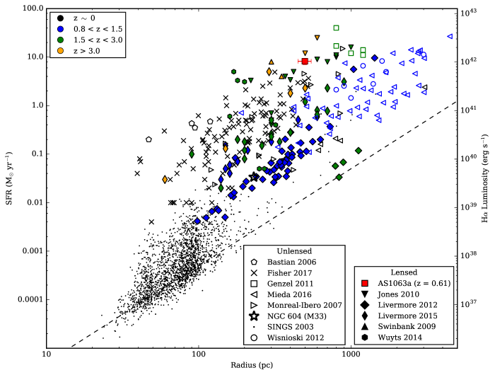
Figure 14: Relation between SFR and the radius of H ii regions (adapted from; Wisnioski et al., 2012; Livermore et al., 2012). The red point is the H ii region from AS1063a at $z=0.61$. The other points are all galaxies above $z>0.8$, color coded by redshift, by combining samples of lensed (solid color symbols; Swinbank et al., 2009; Jones et al., 2010b; Livermore et al., 2012; Wuyts et al., 2014; Livermore et al., 2015) and unlensed (open symbols; Förster Schreiber et al., 2011b; Wisnioski et al., 2012; Mieda et al., 2016) galaxies. The grey points are from SINGS galaxies (Kennicutt et al., 2003). The open black symbols are giant H ii regions found at $z\sim 0$ in Antennae galaxies (Bastian et al., 2006) and ULIRGs (Monreal-Ibero et al., 2007). The black star is the giant H ii region NGC 604 found in M33 (Relaño & Kennicutt, 2009). The black x’s are large star-forming clumps from nearby galaxies (Fisher et al., 2017). The dashed line represents a line of constant H$\alpha$ surface brightness, which is proportional to R².

Local star forming galaxies (from the SINGS sample) appear to fall on a surface brightness empirical relation, where as a clump becomes brighter, it also gets larger. It has been suggested that this relation evolves with redshift in galaxies along the “main sequence”, where higher redshift clumps are more luminous than lower redshift clumps for a given size (Livermore et al., 2012, 2015). This evolution may be driven by a galaxy’s gas fraction where the higher redshift galaxies are found to have higher gas fractions than the local galaxies. However, Mieda et al. (2016), found large resolved clumps (using IFS) in high redshift ($z\sim 1$) galaxies, with wide range of SFRs, which appear to be scaled up versions of local H II regions. Additionally, Johnson et al. (2017b) finds that for a $z=2.48$ galaxy with a low star formation rate (9 M${}_{\sun}\ \rm yr^{-1}$) it contains star forming clumps that are 30 - 50 pc in size. This hints that there is a another process at work. Cosens et al. (2018) recently suggested that there is no redshift evolution in the current clump samples, and that there are really two populations of star forming clumps. The populations can be divided based on whether or not a galaxy is undergoing a starburst (i.e. $\Sigma_{\rm SFR}$).

Another key feature is that the clump in AS1063a appears to have formed in isolation (in-situ). As we show in §4.2.4 the clump appears to be embedded in a rotating disk with no evidence of interaction. This is typical of the clumps found at high redshift ($z>2$) but uncommon for local galaxies. For galaxies at low redshift it is found that massive luminous star forming regions are induced by the interacting galaxies. It is suggested that the conditions at higher redshift, higher gas fractions and cold flow accretion, may be responsible for clumps forming in isolation, perhaps due to gravitational instability. They could also be short lived features, as work from Dekel et al. (2009), Genzel et al. (2011) and Guo et al. (2012) has suggested that clumps can migrate or diffuse within 0.1–1 Gyr. We also know that H$\alpha$ emission traces recent star formation (Kennicutt & Evans, 2012) within the last 3-10 Myr.

It would be expected that such a clump at this redshift would be quite rare. However, two of the largest and brightest clumps in the Livermore et al. (2012) sample ($z=1-1.5$) are at redshift $z=1.01$ (A773). These clumps are more comparable to the size and luminosity of clumps in the Jones et al. (2010b) sample at redshift $z\sim 2$ and the Wisnioski et al. (2012) sample (WiggleZ). Recent work by Guo et al. (2015) has shown that a galaxies’ stellar mass determines the frequency of clumps found from redshifts $z=0.5-2$. The clump fraction remains constant for galaxies with a smaller stellar mass, whereas the clump fraction decreases with time over the redshift range for higher stellar mass galaxies.

5 Conclusions

In this paper we present the results of the infrared/submillimeter survey of the core of the massive galaxy cluster AS1063. Three bright 24 $\micron$ detected sources near (r$<$30″) the cluster core of AS1063 stand out in the survey. Two of the sources are cluster members (AS1063b and AS1063c) with recent star formation. The third source is a lensed galaxy at $z=0.61$ (AS1063a). We also present evidence that AS1063a contains a giant H II region that is about a kiloparsec in diameter and 2 orders of magnitude more luminous than typical local H II regions, with strong Balmer line emission (H$\alpha$-H8) and forbidden line emission ([O II] $\lambda$3727, [O III] $\lambda\lambda$4959,5007, and [Ne III]).

The main conclusions in this paper are the following:

• We discover a gravitationally lensed galaxy (AS1063a) with a giant luminous H II region (D = 1 kpc, SFR$\sim$10 M${}_{\sun}\ \rm yr^{-1}$) at $z=0.61$. It appears to be a single clump with no additional clumps resolved within it larger than 90 pc (ACS resolution with the aide of gravitational lensing).

• The kinematics of the [O II]$\lambda 3727$ doublet indicate that the giant H II region is part of a rotating disk. There is no evidence of any nearby galaxies interacting with AS1063a which suggests that this H II region formed in-situ.

• We find a significant offset between the 24 $\micron$ emission and center of AS1063a, in which it falls between the bulge and H II region of the galaxy. When fitting the extended 24 $\micron$ emission, we find that it is likely that half of the star formation in AS1063a is coming from the giant H II region. Though we cannot rule out the possibility of a obscured star forming region, due to the degeneracy of the fits to the MIPS PSF.

• Using both a dust-to-gas ratio and kinematics of the galaxy rotation we are able to determine the gas fraction, f_gas = 0.13${}^{+0.06}_{-0.04}$, which is typical for LIRGs at that redshift. At $z\sim 2$ gas fractions are normally 0.3 – 0.8.

• Assuming that about half of the star formation comes from the H II region and using the gas fraction, implies that the depletion timescale for the H II region is roughly between 70-230 Myr. Incorporating the stellar age, the lifetime of the H II is predicted to be 280-920 Myr, which makes it short-lived.

The H II region in AS1063a is more luminous than local analogs and is unexpectedly luminous for its redshift, resembling an H II region at $z\sim 2$. This could potentially be a rare occurrence, however in the Livermore et al. (2012) sample, two star forming clumps found in a lensed galaxy in A773, have similar luminosity and size at $z=1.01$. In addition, the giant H II region in AS1063a appears to have formed in isolation, and to have been not induced by a merger. Unlike giant star forming regions in the local Universe, the giant H II region in AS1063a appears more like the ones found in redshift $z\sim 2$ galaxies. Even though recent studies (Guo et al., 2015) have determined the fraction of clumps in field galaxies at redshifts $z=0.5-2$, they are typically unresolved. Larger samples of gravitationally lensed IR galaxies will be necessary to determine the distribution of sizes and luminosities of resolved star forming regions.

Appendix A 24 $\mu$m Selected Galaxies with Spectroscopic Redshifts

In Table 9 and 10 we list the 71 Spitzer/MIPS 24 $\micron$ sources in this sample; 61 of which were targeted with Magellan/LDSS-3 and the redshifts for 10 are from the literature Gómez et al. (2012); Karman et al. (2015); Caminha et al. (2016); Rawle et al. (2016); Karman et al. (2017); Connor et al. (2017). Spectroscopic redshifts for all of the Spitzer/MIPS 24 $\micron$ counterparts are listed in Table 9. The Spitzer/MIPS 24 $\micron$ sources targeted with LDSS-3 but a spectroscopic redshift was unable to be determined are listed in Table 10. For the sources targeted with LDSS-3, a spectroscopic redshift was determined with either one or more emission or absorption features. The redshifts for twenty-three 24 $\mu$m sources were previously unknown, mostly between the redshifts $0.6<z<1.4$. The emission lines detected are listed in Table 9 for the LDSS-3 sample. We adopt similar spectroscopic quality codes as the DEEP2 survey. The redshift quality codes are defined as the following; $z_{q}$ of 2 is a single emission or absorption feature where the redshift is dubious, $z_{q}$ of 3 there is a few emission or absorption features where the redshift is secure, and a $z_{q}$ of 4 several emission and absorption features and the redshift is very secure.

Figure 15 shows the positions of the galaxies from our sample and the literature. From the spectroscopic sample, we find that 29 galaxies are in the background, 15 are cluster members and 5 are foreground galaxies. For one of the sources the correct counterpart is ambiguous, there are two galaxies within 1.58″ of each other and they both fall within the LDSS-3 slit. Based on the distance from the optical counterparts to the 24 $\micron$ source, the lower redshift galaxy ($z=0.474$) appears to be the more likely candidate of the 24 $\micron$ emission. Of the 29 background galaxies; 12 have redshifts $z>1$, one of which is within the central arcmin of the cluster center. Of the 24 galaxies with previously unknown redshifts, 20 of the galaxies are found in the background of the cluster.

We also identify 5 galaxies at redshift $z\sim 0.6$, one of which is discovered in Gómez et al. (2012). The spatial distance between these galaxies and AS1063a, when accounting for the deflection caused by gravitational lensing, are 230, 470, 580 and 980 kpc. This study, Gómez et al. (2012) and Karman et al. (2015) identify 6 galaxies at $z\sim 0.6$ all within 2.4′ of each other and a $\Delta$v of 2400 km s^-1 (5 within 1.4′ and with $\Delta$v of 370 km s^-1). Gruen et al. (2013) uses weak lensing to suggest that there is a background cluster at $z\sim 0.6$, offset by 14.5′ from AS1063. This could potentially be an infalling group, however this is speculative, more wide field spectroscopy is needed to determine the size and structure of the suspected background cluster at $z\sim 0.6$.

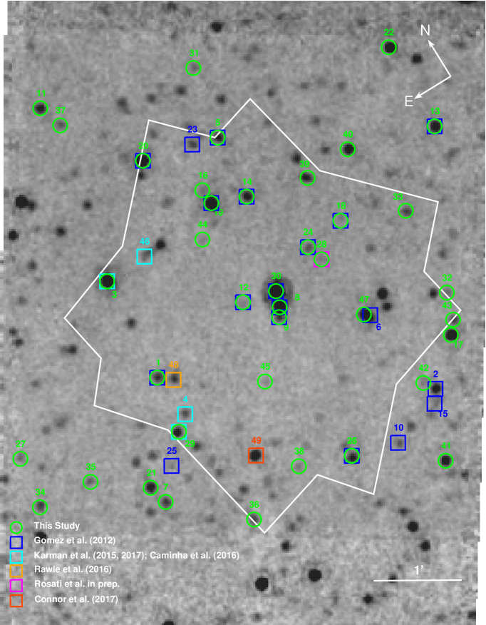
Figure 15: Spitzer/MIPS 24$\micron$ image showing the central 5′$\times$5′ FOV of AS1063. All of the 24 $\micron$ sources that are marked have a redshift. The green circles mark the positions of 24 $\micron$ selected galaxies targeted by this study. The squares mark the positions of the galaxies with redshifts from Gómez et al. (2012); Karman et al. (2015); Caminha et al. (2016); Rawle et al. (2016); Connor et al. (2017); Karman et al. (2017) and Rosati et al. in prep. which are now known to have 24 $\micron$ emission. Source 30 is AS1063a (the main focus of this paper), source 8 is AS1063b and source 9 is AS1063c. The white polygon represents the CLASH ACS FOV.

Table 9: Spectroscopic Redshifts of 24 $\micron$ Selected Galaxies

ID	R.A.	Decl.	F24µm(mJy)	z	zq	Ref.	Emission Lines
1	22:48:51.250	-44:32:04.14	0.222$\pm$0.010	0.082	4	a	[OII], H$\beta$, [OIII]λ4959,5007, HeI, [OI], H$\alpha$, [NII]λ6548,6583, [SII], [ArIII]
2	22:48:36.308	-44:33:52.23	0.356$\pm$0.013	0.198		a,g	$\cdots$
3	22:48:50.728	-44:30:49.15	1.234$\pm$0.017	0.211	4	b,d	[OII], [NeIII], H$\gamma$, H$\beta$, [OIII]λ4959,5007, H$\alpha$, [NII]λ6548,6583, [SII]
4	22:48:50.961	-44:32:35.86	0.102$\pm$0.007	0.237		b,d,g	$\cdots$
5	22:48:39.744	-44:30:04.87	0.220$\pm$0.013	0.275	4	a	[OII], H$\beta$, [OIII]λ4959,5007, H$\alpha$, [NII]λ6548,6583, [SII]
6	22:48:37.389	-44:32:45.05	0.725$\pm$0.016	0.331		a,g	$\cdots$
7	22:48:55.030	-44:33:20.36	0.250$\pm$0.016	0.332	4		[OII], H$\delta$, H$\gamma$, H$\beta$, [OIII]λ5007, HeI, H$\alpha$, [NII]λ6548,6583, [SII]
8	22:48:42.113	-44:32:07.39	0.769$\pm$0.012	0.337	4	a,b	[OII], H$\beta$, [OIII]λ4363,4959,5007, H$\alpha$, [NII]λ6548,6583, [SII]
9	22:48:42.480	-44:32:12.99	0.270$\pm$0.034	0.337	4	a,b	[OII], H$\beta$, [OIII]λ5007, H$\alpha$, [NII]λ6548,6583
10	22:48:40.205	-44:34:10.30	0.111$\pm$0.010	0.338		a,g	$\cdots$
11	22:48:48.503	-44:28:42.90	0.257$\pm$0.012	0.341	4		[OII], H$\alpha$, [NII]λ6548,6583, [SII]
12	22:48:43.960	-44:31:51.02	0.099$\pm$0.005	0.347	4	a,b,h	$\cdots$
13	22:48:27.407	-44:31:17.28	0.342$\pm$0.012	0.348	4	a	[OII], H$\beta$, H$\alpha$, [NII]λ6548,6583, [SII]
14	22:48:40.158	-44:30:50.17	0.256$\pm$0.014	0.351	4	a	[OII], H$\beta$, [OIII]λ5007, H$\alpha$, [NII]λ6548,6583, [SII]
15	22:48:36.857	-44:34:00.61	0.149$\pm$0.006	0.353		a,g	$\cdots$
16	22:48:42.379	-44:30:30.28	0.135$\pm$0.005	0.354	4	h	$\cdots$
17	22:48:33.617	-44:33:26.01	0.511$\pm$0.012	0.335	4		H$\beta$, H$\alpha$, [NII]λ6548,6583, [SII]
18	22:48:35.806	-44:31:38.61	0.063$\pm$0.005	0.335	4	a	[OIII]λ5007, H$\alpha$,[NII]λ6583 [SII]
19	22:48:42.325	-44:30:41.12	0.801$\pm$0.017	0.355	4	a	[OII], [NeIII],[OIII]λ4959,5007, H$\alpha$, [NII]λ6548,6583, [SII]
20	22:48:44.647	-44:29:51.22	0.728$\pm$0.014	0.355	4	a	[OII], H$\alpha$, [NII]λ6548,6583, [SII]
21	22:48:55.368	-44:33:06.54	0.304$\pm$0.015	0.403	4		[OII], H$\beta$, [OIII]λ4959,5007, H$\alpha$, [NII]λ6548,6583
22	22:48:27.245	-44:30:13.99	0.406$\pm$0.011	0.453	4		[OII], H$\beta$, H$\alpha$, [NII]λ6548,6583, [SII]
23	22:48:41.380	-44:29:59.64	0.122$\pm$0.010	0.454		a,g	$\cdots$
24	22:48:38.502	-44:31:42.29	0.128$\pm$0.012	0.457	4	a	[OII], H$\beta$, [OIII]λ4959,5007, H$\alpha$, [NII]λ6548,6583, [SII]
25	22:48:53.479	-44:33:01.29	0.093$\pm$0.005	0.457		a,g	$\cdots$
26	22:48:43.200	-44:34:01.11	0.280$\pm$0.014	0.474	4		[OII], H$\beta$, [OIII]λ5007, H$\alpha$
			0.280$\pm$0.014	0.609	3	a	H$\beta$
27	22:49:01.556	-44:32:01.95	0.049$\pm$0.005	0.570	4		[OII], [OIII]λ5007
28	22:48:38.171	-44:31:54.38	0.092$\pm$0.005	0.610	3	e	[OII]
29	22:48:51.905	-44:32:43.89	0.244$\pm$0.012	0.610	4	b,d,h	$\cdots$
30	22:48:41.760	-44:31:56.53	2.223$\pm$0.015	0.611	4	a,b	[OII], [NeIII], H8, H$\epsilon$, H$\delta$, H$\gamma$, H$\beta$, [OIII]λ4959,5007
31	22:48:38.707	-44:29:15.03	0.051$\pm$0.007	0.622	4		[OII], [NeIII], H8, H$\epsilon$, H$\delta$, H$\gamma$, H$\beta$, [OIII]λ4959,5007
32	22:48:32.400	-44:32:59.69	0.065$\pm$0.007	0.745	3		[OII], [NeIII], H$\beta$
33	22:48:31.871	-44:31:56.48	0.167$\pm$0.013	0.746	4		[OII], [NeIII], H$\delta$, H$\gamma$, H$\beta$, [OIII]λ4959,5007
34	22:49:02.129	-44:32:37.61	0.206$\pm$0.013	0.746	3		[OII], H$\beta$
35	22:48:58.482	-44:32:41.14	0.083$\pm$0.010	0.960	2		[OII]
36	22:48:50.756	-44:34:02.97	0.128$\pm$0.008	0.969	2		[OII]
37	22:48:47.995	-44:29:00.28	0.070$\pm$0.007	0.974	2		[OII], H$\gamma$
38	22:48:46.472	-44:33:47.95	0.044$\pm$0.007	1.033	2		[OII]
39	22:48:36.162	-44:31:01.35	0.264$\pm$0.015	1.034	2		[OII]
40	22:48:32.980	-44:30:59.08	0.316$\pm$0.013	1.035	2		[OII]
41	22:48:38.196	-44:34:38.27	0.399$\pm$0.014	1.074	4		[OII]
42	22:48:36.767	-44:33:44.35	0.108$\pm$0.006	1.116	3		[OII], [NeIII]
43	22:48:32.972	-44:33:17.89	0.138$\pm$0.011	1.241	4		[OII], [NeIII]
44	22:48:44.053	-44:30:59.34	0.074$\pm$0.005	1.241	2		[OII]
45	22:48:45.450	-44:32:45.75	0.048$\pm$0.005	1.285	3		[OII], H$\delta$
46	22:48:47.830	-44:30:48.20	0.191$\pm$0.005	1.427		b,d,g	$\cdots$
47	22:48:37.717	-44:32:42.35	0.725$\pm$0.016	1.440	4		CII]λ2327, [NeIV], MgII, [NeV], [OII], [NeIII]
48	22:48:50.432	-44:32:11.41	0.327$\pm$0.006	1.440		c,d,g	$\cdots$
49	22:48:48.543	-44:33:25.85	0.348$\pm$0.011	2.566		f,g	$\cdots$

Note. — Emission lines in the table are abrevations of the following: [ArIII] - [ArIII]$\lambda 7135$, HeI - HeI$\lambda 5876$, MgII - MgII$\lambda 2796,2804$, [NeIII] - [NeIII]$\lambda 3869$, [NeIV] - [NeIV]$\lambda 2425$, [NeV] - [NeV]$\lambda 3326,3346$, [OI] - [OI]$\lambda 6300$, [OII] - [OII]$\lambda 3727$, [SII] - [SII]$\lambda 6717,6731$

Table 10: 24 $\micron$ Selected Galaxies Targeted without a Redshift

ID	R.A.	Decl.	F24µm(mJy)
50	22:48:38.351	-44:29:43.46	0.146$\pm$0.011
51	22:48:33.829	-44:30:30.27	0.083$\pm$0.009
52	22:48:38.390	-44:33:17.88	0.089$\pm$0.006
53	22:48:51.484	-44:32:59.22	0.153$\pm$0.012
54	22:48:35.514	-44:27:54.21	0.232$\pm$0.014
55	22:48:52.765	-44:29:30.57	0.650$\pm$0.011
56	22:48:36.662	-44:34:19.83	0.072$\pm$0.009
57	22:48:38.959	-44:34:05.20	0.121$\pm$0.010
58	22:48:37.595	-44:34:54.06	0.234$\pm$0.013
59	22:48:26.323	-44:30:46.24	0.077$\pm$0.005
60	22:48:33.278	-44:30:05.67	0.082$\pm$0.008
61	22:48:31.255	-44:30:19.07	0.085$\pm$0.007
62	22:48:29.689	-44:30:35.04	0.030$\pm$0.005
63	22:48:36.515	-44:30:14.18	0.073$\pm$0.009
64	22:48:34.301	-44:30:51.34	0.127$\pm$0.012
65	22:48:40.691	-44:30:41.67	0.094$\pm$0.006
66	22:48:46.584	-44:30:46.90	0.249$\pm$0.009
67	22:48:36.050	-44:32:36.58	0.432$\pm$0.012
68	22:48:50.861	-44:31:22.54	0.130$\pm$0.007
69	22:48:53.780	-44:32:26.19	0.087$\pm$0.009
70	22:49:03.205	-44:32:54.00	0.439$\pm$0.011
71	22:48:23.267	-44:30:38.31	0.078$\pm$0.006

References

- Armus et al. (1990) Armus, L., Heckman, T. M., & Miley, G. K. 1990, ApJ, 364, 471
- Balestra et al. (2013) Balestra, I., Vanzella, E., Rosati, P., et al. 2013, A&A, 559, L9
- Barnes & Sellwood (2003) Barnes, E. I., & Sellwood, J. A. 2003, AJ, 125, 1164
- Barnes & Hernquist (1991) Barnes, J. E., & Hernquist, L. E. 1991, ApJ, 370, L65
- Bastian et al. (2006) Bastian, N., Emsellem, E., Kissler-Patig, M., & Maraston, C. 2006, A&A, 445, 471
- Bertin & Arnouts (1996) Bertin, E., & Arnouts, S. 1996, A&AS, 117, 393
- Boone et al. (2013) Boone, F., Clément, B., Richard, J., et al. 2013, A&A, 559, L1
- Bournaud et al. (2007) Bournaud, F., Elmegreen, B. G., & Elmegreen, D. M. 2007, ApJ, 670, 237
- Bruzual & Charlot (2003) Bruzual, G., & Charlot, S. 2003, MNRAS, 344, 1000
- Caminha et al. (2016) Caminha, G. B., Grillo, C., Rosati, P., et al. 2016, A&A, 587, A80
- Cava et al. (2018) Cava, A., Schaerer, D., Richard, J., et al. 2018, Nature Astronomy, 2, 76
- Chary & Elbaz (2001) Chary, R., & Elbaz, D. 2001, ApJ, 556, 562
- Combes et al. (2012) Combes, F., Rex, M., Rawle, T. D., et al. 2012, A&A, 538, L4
- Connor et al. (2017) Connor, T., Donahue, M., Kelson, D. D., et al. 2017, ApJ, 848, 37
- Cosens et al. (2018) Cosens, M., Wright, S. A., Mieda, E., et al. 2018, ApJ, 869, 11
- Courteau (1997) Courteau, S. 1997, AJ, 114, 2402
- Cowie et al. (1995) Cowie, L. L., Hu, E. M., & Songaila, A. 1995, AJ, 110, 1576
- da Cunha et al. (2013) da Cunha, E., Groves, B., Walter, F., et al. 2013, ApJ, 766, 13
- Daddi et al. (2010) Daddi, E., Bournaud, F., Walter, F., et al. 2010, ApJ, 713, 686
- Dekel et al. (2009) Dekel, A., Sari, R., & Ceverino, D. 2009, ApJ, 703, 785
- Dressler et al. (2011) Dressler, A., Bigelow, B., Hare, T., et al. 2011, PASP, 123, 288
- Egami et al. (2010) Egami, E., Rex, M., Rawle, T. D., et al. 2010, A&A, 518, L12
- Elmegreen et al. (2004a) Elmegreen, D. M., Elmegreen, B. G., & Hirst, A. C. 2004a, ApJ, 604, L21
- Elmegreen et al. (2004b) Elmegreen, D. M., Elmegreen, B. G., & Sheets, C. M. 2004b, ApJ, 603, 74
- Fazio et al. (2004) Fazio, G. G., Hora, J. L., Allen, L. E., et al. 2004, ApJS, 154, 10
- Fernández et al. (2016) Fernández, X., Gim, H. B., van Gorkom, J. H., et al. 2016, ApJ, 824, L1
- Fisher et al. (2017) Fisher, D. B., Glazebrook, K., Damjanov, I., et al. 2017, MNRAS, 464, 491
- Förster Schreiber et al. (2011a) Förster Schreiber, N. M., Shapley, A. E., Erb, D. K., et al. 2011a, ApJ, 731, 65
- Förster Schreiber et al. (2009) Förster Schreiber, N. M., Genzel, R., Bouché, N., et al. 2009, ApJ, 706, 1364
- Förster Schreiber et al. (2011b) Förster Schreiber, N. M., Shapley, A. E., Genzel, R., et al. 2011b, ApJ, 739, 45
- Frye et al. (2012) Frye, B. L., Hurley, M., Bowen, D. V., et al. 2012, ApJ, 754, 17
- Geach et al. (2011) Geach, J. E., Smail, I., Moran, S. M., et al. 2011, ApJ, 730, L19
- Genzel et al. (2011) Genzel, R., Newman, S., Jones, T., et al. 2011, ApJ, 733, 101
- Gómez et al. (2012) Gómez, P. L., Valkonen, L. E., Romer, A. K., et al. 2012, AJ, 144, 79
- Greve et al. (2012) Greve, T. R., Vieira, J. D., Weiß, A., et al. 2012, ApJ, 756, 101
- Griffin et al. (2010) Griffin, M. J., Abergel, A., Abreu, A., et al. 2010, A&A, 518, L3
- Gruen et al. (2013) Gruen, D., Brimioulle, F., Seitz, S., et al. 2013, MNRAS, 432, 1455
- Guo et al. (2012) Guo, Y., Giavalisco, M., Ferguson, H. C., Cassata, P., & Koekemoer, A. M. 2012, ApJ, 757, 120
- Guo et al. (2015) Guo, Y., Ferguson, H. C., Bell, E. F., et al. 2015, ApJ, 800, 39
- Henry & Worthey (1999) Henry, R. B. C., & Worthey, G. 1999, PASP, 111, 919
- Hildebrand (1983) Hildebrand, R. H. 1983, QJRAS, 24, 267
- Hodge et al. (2016) Hodge, J. A., Swinbank, A. M., Simpson, J. M., et al. 2016, ApJ, 833, 103
- Holmberg (1958) Holmberg, E. 1958, Meddelanden fran Lunds Astronomiska Observatorium Serie II, 136, 1
- Holtzman et al. (1992) Holtzman, J. A., Faber, S. M., Shaya, E. J., et al. 1992, AJ, 103, 691
- Houck et al. (2004) Houck, J. R., Roellig, T. L., van Cleve, J., et al. 2004, ApJS, 154, 18
- Johnson et al. (2017a) Johnson, T. L., Sharon, K., Gladders, M. D., et al. 2017a, ApJ, 843, 78
- Johnson et al. (2017b) Johnson, T. L., Rigby, J. R., Sharon, K., et al. 2017b, ApJ, 843, L21
- Jones et al. (2010a) Jones, T., Ellis, R., Jullo, E., & Richard, J. 2010a, ApJ, 725, L176
- Jones et al. (2013) Jones, T., Ellis, R. S., Richard, J., & Jullo, E. 2013, ApJ, 765, 48
- Jones et al. (2010b) Jones, T. A., Swinbank, A. M., Ellis, R. S., Richard, J., & Stark, D. P. 2010b, MNRAS, 404, 1247
- Jullo & Kneib (2009) Jullo, E., & Kneib, J.-P. 2009, MNRAS, 395, 1319
- Jullo et al. (2007) Jullo, E., Kneib, J.-P., Limousin, M., et al. 2007, New Journal of Physics, 9, 447
- Karman et al. (2015) Karman, W., Caputi, K. I., Grillo, C., et al. 2015, A&A, 574, A11
- Karman et al. (2017) Karman, W., Caputi, K. I., Caminha, G. B., et al. 2017, A&A, 599, A28
- Kauffmann et al. (2003) Kauffmann, G., Heckman, T. M., Tremonti, C., et al. 2003, MNRAS, 346, 1055
- Kelson (2003) Kelson, D. D. 2003, PASP, 115, 688
- Kennicutt & Evans (2012) Kennicutt, R. C., & Evans, N. J. 2012, ARA&A, 50, 531
- Kennicutt (1998) Kennicutt, Jr., R. C. 1998, ARA&A, 36, 189
- Kennicutt et al. (2003) Kennicutt, Jr., R. C., Armus, L., Bendo, G., et al. 2003, PASP, 115, 928
- Kewley & Ellison (2008) Kewley, L. J., & Ellison, S. L. 2008, ApJ, 681, 1183
- Kewley et al. (2001) Kewley, L. J., Heisler, C. A., Dopita, M. A., & Lumsden, S. 2001, ApJS, 132, 37
- Kneib et al. (1996) Kneib, J.-P., Ellis, R. S., Smail, I., Couch, W. J., & Sharples, R. M. 1996, ApJ, 471, 643
- Krist et al. (2011) Krist, J. E., Hook, R. N., & Stoehr, F. 2011, in Proc. SPIE, Vol. 8127, Optical Modeling and Performance Predictions V, 81270J
- Kruegel & Siebenmorgen (1994) Kruegel, E., & Siebenmorgen, R. 1994, A&A, 288, 929
- Kümmel et al. (2009) Kümmel, M., Walsh, J. R., Pirzkal, N., Kuntschner, H., & Pasquali, A. 2009, PASP, 121, 59
- Leroy et al. (2011) Leroy, A. K., Bolatto, A., Gordon, K., et al. 2011, ApJ, 737, 12
- Livermore et al. (2012) Livermore, R. C., Jones, T., Richard, J., et al. 2012, MNRAS, 427, 688
- Livermore et al. (2015) Livermore, R. C., Jones, T. A., Richard, J., et al. 2015, MNRAS, 450, 1812
- Madau et al. (1998) Madau, P., Pozzetti, L., & Dickinson, M. 1998, ApJ, 498, 106
- Magdis et al. (2012) Magdis, G. E., Daddi, E., Sargent, M., et al. 2012, ApJ, 758, L9
- Mainali et al. (2017) Mainali, R., Kollmeier, J. A., Stark, D. P., et al. 2017, ApJ, 836, L14
- Maughan et al. (2008) Maughan, B. J., Jones, C., Forman, W., & Van Speybroeck, L. 2008, ApJS, 174, 117
- McLeod et al. (2012) McLeod, B., Fabricant, D., Nystrom, G., et al. 2012, PASP, 124, 1318
- Meurer et al. (1995) Meurer, G. R., Heckman, T. M., Leitherer, C., et al. 1995, AJ, 110, 2665
- Mieda et al. (2016) Mieda, E., Wright, S. A., Larkin, J. E., et al. 2016, ApJ, 831, 78
- Mihos & Hernquist (1996) Mihos, J. C., & Hernquist, L. 1996, ApJ, 464, 641
- Mirabel & Sanders (1989) Mirabel, I. F., & Sanders, D. B. 1989, ApJ, 340, L53
- Monna et al. (2014) Monna, A., Seitz, S., Greisel, N., et al. 2014, MNRAS, 438, 1417
- Monreal-Ibero et al. (2007) Monreal-Ibero, A., Colina, L., Arribas, S., & García-Marín, M. 2007, A&A, 472, 421
- Moustakas et al. (2010) Moustakas, J., Kennicutt, Jr., R. C., Tremonti, C. A., et al. 2010, ApJS, 190, 233
- Noeske et al. (2007) Noeske, K. G., Weiner, B. J., Faber, S. M., et al. 2007, ApJ, 660, L43
- Papadopoulos et al. (2000) Papadopoulos, P. P., Röttgering, H. J. A., van der Werf, P. P., et al. 2000, ApJ, 528, 626
- Peng et al. (2002) Peng, C. Y., Ho, L. C., Impey, C. D., & Rix, H.-W. 2002, AJ, 124, 266
- Peng et al. (2010) —. 2010, AJ, 139, 2097
- Pérez-González et al. (2008) Pérez-González, P. G., Rieke, G. H., Villar, V., et al. 2008, ApJ, 675, 234
- Pérez-González et al. (2013) Pérez-González, P. G., Cava, A., Barro, G., et al. 2013, ApJ, 762, 46
- Pettini & Pagel (2004) Pettini, M., & Pagel, B. E. J. 2004, MNRAS, 348, L59
- Piazzo et al. (2015) Piazzo, L., Calzoletti, L., Faustini, F., et al. 2015, MNRAS, 447, 1471
- Pilbratt et al. (2010) Pilbratt, G. L., Riedinger, J. R., Passvogel, T., et al. 2010, A&A, 518, L1
- Poglitsch et al. (2010) Poglitsch, A., Waelkens, C., Geis, N., et al. 2010, A&A, 518, L2
- Postman et al. (2012) Postman, M., Coe, D., Benítez, N., et al. 2012, ApJS, 199, 25
- Rawle et al. (2012) Rawle, T. D., Edge, A. C., Egami, E., et al. 2012, ApJ, 747, 29
- Rawle et al. (2014) Rawle, T. D., Egami, E., Bussmann, R. S., et al. 2014, ApJ, 783, 59
- Rawle et al. (2016) Rawle, T. D., Altieri, B., Egami, E., et al. 2016, MNRAS, 459, 1626
- Relaño & Kennicutt (2009) Relaño, M., & Kennicutt, Jr., R. C. 2009, ApJ, 699, 1125
- Rex et al. (2010) Rex, M., Rawle, T. D., Egami, E., et al. 2010, A&A, 518, L13
- Richard et al. (2014) Richard, J., Jauzac, M., Limousin, M., et al. 2014, MNRAS, 444, 268
- Rieke et al. (2009) Rieke, G. H., Alonso-Herrero, A., Weiner, B. J., et al. 2009, ApJ, 692, 556
- Rieke et al. (2004) Rieke, G. H., Young, E. T., Engelbracht, C. W., et al. 2004, ApJS, 154, 25
- Rigby & Rieke (2004) Rigby, J. R., & Rieke, G. H. 2004, ApJ, 606, 237
- Rigby et al. (2017) Rigby, J. R., Johnson, T. L., Sharon, K., et al. 2017, ApJ, 843, 79
- Rodighiero et al. (2011) Rodighiero, G., Daddi, E., Baronchelli, I., et al. 2011, ApJ, 739, L40
- Rupke et al. (2010) Rupke, D. S. N., Kewley, L. J., & Chien, L.-H. 2010, ApJ, 723, 1255
- Sanders & Mirabel (1996) Sanders, D. B., & Mirabel, I. F. 1996, ARA&A, 34, 749
- Sandstrom et al. (2013) Sandstrom, K. M., Leroy, A. K., Walter, F., et al. 2013, ApJ, 777, 5
- Santini et al. (2010) Santini, P., Maiolino, R., Magnelli, B., et al. 2010, A&A, 518, L154
- Schmidt et al. (2014) Schmidt, K. B., Treu, T., Brammer, G. B., et al. 2014, ApJ, 782, L36
- Schweizer (1987) Schweizer, F. 1987, in Nearly Normal Galaxies. From the Planck Time to the Present, ed. S. M. Faber, 18–25
- Siringo et al. (2009) Siringo, G., Kreysa, E., Kovács, A., et al. 2009, A&A, 497, 945
- Smith et al. (2007) Smith, J. D. T., Draine, B. T., Dale, D. A., et al. 2007, ApJ, 656, 770
- Sofue et al. (1999) Sofue, Y., Tutui, Y., Honma, M., et al. 1999, ApJ, 523, 136
- Swinbank et al. (2009) Swinbank, A. M., Webb, T. M., Richard, J., et al. 2009, MNRAS, 400, 1121
- Thornley et al. (2000) Thornley, M. D., Schreiber, N. M. F., Lutz, D., et al. 2000, ApJ, 539, 641
- Tody (1986) Tody, D. 1986, in Proc. SPIE, Vol. 627, Instrumentation in astronomy VI, ed. D. L. Crawford, 733
- Tody (1993) Tody, D. 1993, in Astronomical Society of the Pacific Conference Series, Vol. 52, Astronomical Data Analysis Software and Systems II, ed. R. J. Hanisch, R. J. V. Brissenden, & J. Barnes, 173
- Treu et al. (2015) Treu, T., Schmidt, K. B., Brammer, G. B., et al. 2015, ApJ, 812, 114
- Werner et al. (2004) Werner, M. W., Roellig, T. L., Low, F. J., et al. 2004, ApJS, 154, 1
- Whitaker et al. (2012) Whitaker, K. E., van Dokkum, P. G., Brammer, G., & Franx, M. 2012, ApJ, 754, L29
- Whitmore et al. (1993) Whitmore, B. C., Schweizer, F., Leitherer, C., Borne, K., & Robert, C. 1993, AJ, 106, 1354
- Williamson et al. (2011) Williamson, R., Benson, B. A., High, F. W., et al. 2011, ApJ, 738, 139
- Wisnioski et al. (2012) Wisnioski, E., Glazebrook, K., Blake, C., et al. 2012, MNRAS, 422, 3339
- Wisnioski et al. (2013) Wisnioski, E., Glazebrook, K., Blake, C., & Swinbank, A. M. 2013, MNRAS, 436, 266
- Wong et al. (2012) Wong, K. C., Ammons, S. M., Keeton, C. R., & Zabludoff, A. I. 2012, ApJ, 752, 104
- Wuyts et al. (2014) Wuyts, E., Rigby, J. R., Gladders, M. D., & Sharon, K. 2014, ApJ, 781, 61
- Yuan et al. (2011) Yuan, T.-T., Kewley, L. J., Swinbank, A. M., Richard, J., & Livermore, R. C. 2011, ApJ, 732, L14