Crystal field coefficients for yttrium analogues of rare-earth/transition-metal magnets using density-functional theory in the projector-augmented wave formalism

Abstract

We present a method of calculating crystal field coefficients of rare-earth/transition-metal (RE-TM) magnets within density-functional theory (DFT). The principal idea of the method is to calculate the crystal field potential of the yttrium analogue (“Y-analogue”) of the RE-TM magnet, i.e. the material where the lanthanide elements have been substituted with yttrium. The advantage of dealing with Y-analogues is that the methodological and conceptual difficulties associated with treating the highly-localized 4$f$ electrons in DFT are avoided, whilst the nominal valence electronic structure principally responsible for the crystal field is preserved. In order to correctly describe the crystal field potential in the core region of the atoms we use the projector-augmented wave formalism of DFT, which allows the reconstruction of the full charge density and electrostatic potential. The Y-analogue crystal field potentials are combined with radial 4$f$ charge densities obtained in self-interaction-corrected calculations on the lanthanides to obtain crystal field coefficients. We demonstrate our method on a test set of 10 materials comprising 9 RE-TM magnets and elemental Tb. We show that the calculated easy directions of magnetization agree with experimental observations, including a correct description of the anisotropy within the basal plane of Tb and NdCo₅. We further show that the Y-analogue calculations generally agree quantitatively with previous calculations using the open-core approximation to treat the 4$f$ electrons, and argue that our simple approach may be useful for large-scale computational screening of new magnetic materials.

1 Introduction

Rare-earth/transition-metal (RE-TM) compounds, particularly those containing neodymium, samarium and dysprosium, are the highest performing permanent magnets on the commercial market [1, 2]. The key factor underpinning the success of these materials is the possibility of obtaining a huge magnetocrystalline anisotropy (MCA), i.e. a preferential direction for an object to be magnetized independent of its macroscopic shape [3], which originates from the highly-localized 4$f$ electrons of the lanthanide elements. Specifically, the unfilled shell of 4$f$ electrons forms a non-spherically symmetric charge cloud which sits in the (also non-spherically symmetric) crystal potential. The interaction between the 4$f$ cloud and the crystal potential, and the interaction between the spin and orbital degrees of freedom of the 4$f$ electrons themselves, results in a strong coupling of the RE magnetism to the crystal potential [4]. The spin-spin RE-TM interaction further couples the magnetic moments of RE to those of the transition metals iron or cobalt [5]. The TM provides a large saturation magnetization and high Curie temperature, which combine with the high MCA to form an excellent permanent magnet [6].

Experimental research into RE-TM permanent magnets has been carried out for over 50 years [7, 8, 9, 10, 11]. Computational research, particularly that based on parameter-free, “first-principles” methods, is a younger field by comparison [12]. However, the growth of computing power and a more widespread availability of modelling codes has led to a rapid increase in recent years of computational works aimed not only at understanding current RE-TM permanent magnets but also predicting the properties of new materials yet to be synthesized experimentally [13, 14, 15, 16, 17, 18, 19, 20, 21, 22, 23, 24, 25, 26]. Here a first-principles approach is highly desirable, since the novel materials may require visiting a previously unexplored parameter space where the reliability of empirical models is unknown.

However, an enduring challenge presented by RE-TM magnets for first-principles calculations is how to simultaneously describe accurately the itinerant electrons of the TM and the highly-localized 4$f$ electrons of the lanthanide. Practical implementations of density-functional theory (DFT) [27], a first-principles methodology which is highly popular due to its versatility and accuracy, require approximating the exchange-correlation (XC) contribution to the total energy of the electrons. Approximations based on the local spin density and the homogeneous electron gas (LSDA/GGA) work very well for itinerant electrons and form the basis of all widely-available DFT codes [28, 29]. Unfortunately, LSDA/GGA XC functionals do not describe the lanthanide elements well, with the 4$f$ electrons being too delocalized [30].

In a previous publication [31], we discussed some different approaches which attempt to correct the LSDA/GGA description of $4f$ electrons. These approaches include the “open core” scheme [32], which effectively removes the 4$f$ states from the valence band and freezes them in the core, dynamical mean-field theory (DMFT) [33], the self-interaction correction [34], and the LSDA/GGA+$U$ scheme [35]. In that publication we chose the (local) self-interaction correction (LSIC) [36] and combined it with the disordered local moment (DLM) picture of finite temperature magnetism [37] to calculate the magnetization and Curie temperatures of the entire series of RE-TM magnets with formula RECo₅ [31]. However, using the same approach to calculate the MCA is problematic, because current LSIC and DLM implementations employ a spherical approximation for the potential at the RE site. The most important contribution to the MCA, i.e. from the crystal potential, is therefore incorrectly described [38].

If we wish to continue with our LSIC/DLM approach to obtain a comprehensive picture of RE-TM magnets, it is apparent that we must augment the original calculations to account for the non-spherical potential at the RE site. Fortunately, an entire theoretical framework has been developed to describe the effects of this asphericity, namely crystal field (CF) theory [39, 40, 41, 42]. Here, the potential at the RE site is expanded in terms of angular functions, and matrix elements with radial 4$f$ wavefunctions are quantified in terms of CF coefficients. Knowledge of the CF coefficients, combined with a description of the finite temperature TM magnetism, can lead to a very detailed picture of RE-TM magnetism [42].

The CF coefficients can be regarded as empirical parameters used to fit experimental data [43], but they can also be calculated. The seminal crystal field models were based on the potential set up by arrays of point charges [39, 40]. The advent of DFT allowed the CF coefficients to be calculated from first principles [12], originally from the electrostatic potential set up by the charge density [44], or later by also including the XC contribution [17, 45, 46, 47]. As usual, the 4$f$ electrons require special treatment, most frequently via the open core scheme [12]. Recent work has also seen the development of sophisticated techniques using DMFT to evaluate CF coefficients [20] or formulating CF theory in a Wannier basis [48].

One reason that a number of different approaches can be found in the literature is that CF theory is essentially empirical, and there is not a unique way of combining it with non-empirical DFT. In particular, in CF theory the 4$f$ electrons are spectators which feel the crystal field but do not themselves influence it [49]. But in a standard DFT calculation the CF potential contains contributions from all electrons, meaning that special treatment of the 4$f$ electron density (e.g. removing the non-spherical components [17]) is required.

Here, we go a step further and present a method where we completely remove the 4$f$ electrons from the crystal field, by calculating the CF potential of the yttrium (Y)-analogue of the RE-TM magnet. Here “Y-analogue” means that have we have replaced all lanthanide atoms with yttrium; for instance, the Y-analogue of Sm₂Co₁₇ is Y₂Co₁₇. This approach is free from the complications of treating the XC energy of the 4$f$ electrons, and produces a potential which does not contain 4$f$ contributions.

Of course, the validity of the approach depends on whether the valence electrons of the lanthanide are well represented by Y. As a bare minimum, the lanthanide must be in a 3+ state, so that the nominal valence configurations agree. For the widely used RE-TM magnets we believe this requirement to be well satisfied [12], but some care will be required in novel materials if the lanthanide is thought to undergo valence fluctuations [25] (for such materials, the open-core approximation would encounter the same problem as the Y-analogue model). In addition, our calculations on the RE³⁺Co₅ compounds revealed a small contribution from $f$-type states around the Fermi level [31] which will be missing for the Y-analogue, as will be any effects due to the (spherically-symmetric) spin polarization of the 4$f$ electrons. Therefore the use of the Y-analogue must be considered an approximation. However, the advantage of making this approximation is then we are free to compute the potential using common LSDA/GGA functionals, using widely available DFT codes.

Our manuscript describes the implementation of the Y-analogue scheme, focusing particularly on two points. The first is that if the chosen DFT code is not an “all-electron” code, i.e. it does not treat core and valence electrons on the same footing, the charge density and potential will be incomplete in the core region of the atoms. By performing the calculations within the projector-augmented wave (PAW) formalism [50], as found in a number of popular codes including Quantum Espresso [51], GPAW [52] and the Vienna Ab initio Simulation Package (VASP) [53], it is possible to restore this core contribution as a post-processing step. In Secs. 2.3–2.6 we describe how this is done.

The second point is that in order to calculate CF coefficients, we require the radial distribution of the 4$f$ electrons. As we discuss in Section 2.7, here we use the spherically symmetric 4$f$ charge density obtained from a separate LSIC calculation. Therefore our method consists of two separate strands, calculated with different codes: one code provides the potential $V({\bf r})$ for the Y-analogue and the other code provides the radial density $n^{0}_{4f}(r)$ for the spherically-symmetric approximated RE-TM compound. Multiplying the two quantities and integrating yields the CF coefficients.

We have used our method to calculate CF coefficients for 10 materials, comprising 9 RE-TM magnets and elemental Tb. Where data is available we compare our calculations to previous work. The data demonstrate all of the correct qualitative trends with respect to experiment, and are in good quantitative agreement with open-core calculations. We therefore present the method as an approximate but simple scheme to calculate CF coefficients.

The rest of our manuscript is organized as follows. In Section 2 we start with a general overview of the crystal field picture and then discuss the specifics of obtaining the potential in the PAW formalism. We also discuss the calculation of the spherically-symmetric 4$f$ density and some of the conventions regarding CF coefficients. In Section 3 we present the calculated CF coefficients and compare to data previously published. Finally in Section 4 we present our conclusions and discuss potential future developments.

2 Theory

2.1 Crystal field picture

As comprehensively explained in Ref. [42] (and references therein), crystal field theory describes atomic-like electrons, which are eigenstates of a central potential and characterized by a set of quantum numbers $|LSJM_{J}\rangle$, perturbed by the CF potential $V({\bf r})$. In the simplest case of a single magnetic sublattice subject to an external field ${\bf B}$ with a spin-orbit coupling quantified by $\lambda$, the CF Hamiltonian is [42]

$$\hat{H}=\lambda\hat{\bf L}\cdot\hat{\bf S}+\mu_{B}(\hat{\bf L}+2\hat{\bf S})\cdot{\bf B}+\sum_{i}V({\bf r_{i}}).$$ (1)

Here ${\bf r_{i}}$ denotes the position of a 4$f$ electron. $V({\bf r})$ can be conveniently expanded in terms of angular functions centred on the RE site. Using the (complex) spherical harmonics $Y_{lm}({\bf\hat{r}})$, this expansion is

$$V({\bf r})=\sum_{lm}V_{lm}(r)Y_{lm}({\bf\hat{r}}).$$ (2)

Matrix elements of $\sum_{i}V({\bf r_{i}})$ are products of radial and angular parts. The angular parts are rewritten and evaluated in terms of operators, and result in the appearance of Stevens coefficients $\alpha_{J}$, $\beta_{J}$ and $\gamma_{J}$, for $l$ = 2, 4, 6 respectively [54]. The radial part of the matrix element forms the CF coefficient, which is the quantity that we aim to calculate in this work:

$$B_{lm}=\left(\frac{2l+1}{4\pi}\right)^{\frac{1}{2}}\int r^{2}n^{0}_{4f}(r)V_{lm}(r)dr$$ (3)

The sign has been defined such that a negative $V_{lm}(r)$ is attractive to an electron, which is the opposite of a conventional electrostatic potential [42]. $n^{0}_{4f}(r)$ is a spherically-symmetric charge density associated with $4f$ electrons which we discuss in Section 2.7, while we discuss the $(2l+1)/(4\pi)$ prefactor in Section 2.8. First, we focus on calculating $V_{lm}(r)$.

2.2 Kohn-Sham potential

As mentioned in the Introduction, the original formulation of CF theory supposed the perturbing potential $V({\bf r})$ to be electrostatic in origin [39]. However, in DFT the many-body system of interacting electrons is mapped onto non-interacting Kohn-Sham (KS) electrons, which experience both an electrostatic and an exchange-correlation potential. As discussed in Ref. [12], it is reasonable to include the XC contribution to the CF potential. However, since the XC potential is spin dependent one must either average over spins [12] or introduce spin-dependent CF coefficients [20]. To keep things general, we take the latter option and slightly modify (3) so that there is a dependence on spin $\sigma(=\uparrow,\downarrow)$:

$$B^{\sigma}_{lm}=\left(\frac{2l+1}{4\pi}\right)^{\frac{1}{2}}\int r^{2}n^{0}_{4f}(r)V^{\sigma}_{lm}(r)dr$$ (4)

where, inverting (2) and inserting the KS potential,

$$V_{lm}^{\sigma}(r) = \int V^{\sigma}_{\mathrm{KS}}({\bf r})Y^{*}_{lm}({\bf\hat{r}})d{\bf\hat{r}}$$ (5)

$$= \int[V_{\mathrm{H}}({\bf r})+V^{\sigma}_{\mathrm{XC}}({\bf r})]Y^{*}_{lm}({\bf\hat{r}})d{\bf\hat{r}}.$$

In our approach $V^{\sigma}_{\mathrm{KS}}({\bf r})$ is the self-consistent KS potential of the Y-analogue of the RE-TM magnet. Above we have split the KS potential into the electrostatic potential $V_{\mathrm{H}}({\bf r})$ (which includes electrostatic electron-electron and electron-nuclear interactions), and the XC potential $V^{\sigma}_{\mathrm{XC}}({\bf r})$.

2.3 PAW

In principle, if one performs an all-electron DFT calculation (particularly using atom-centred basis sets) then extracting $V_{lm}^{\sigma}(r)$ should be straightforward. However, calculations which make some distinction between core and valence electrons, e.g. those using pseudopotentials, do not deal directly with $V^{\sigma}_{\mathrm{KS}}({\bf r})$ but rather with “pseudized” potentials and densities. The advantage of such schemes is that they remove the large computational effort required to describe the rapidly varying electronic wavefunctions in the core region [55].

The projector-augmented wave (PAW) formalism is a popular method to perform such calculations [50]. The full electronic+nuclear charge density is replaced with a pseudo-density $\tilde{\rho}({\bf r})$, which has an associated pseudo-electrostatic potential which solves the Poisson equation $\nabla^{2}\tilde{V}_{\mathrm{H}}({\bf r})=-4\pi\tilde{\rho}({\bf r})$ (Hartree atomic units). The difference between the full and pseudo-density is denoted $\Delta\rho({\bf r})$. For each atom, an augmentation region is defined, which is an atom-centred sphere with a radius of approximately 1–2.5 Bohr radii depending on the atom [56]. Crucially, outside the augmentation spheres the full and pseudo-densities are identical (i.e. $\Delta\rho({\bf r})$ vanishes). Inside, the pseudo-density is constructed such that it has the same multipole moments as the full density. Therefore, the full and pseudo-electrostatic potentials also match each other outside the augmentation spheres [50, 52].

We thus write down a PAW version of (5):

$$V_{lm}^{\sigma}(r) = \int[\tilde{V}_{\mathrm{H}}({\bf r})+V^{\sigma}_{\mathrm{XC}}(n^{\uparrow}({\bf r}),n^{\downarrow}({\bf r}))]Y^{*}_{lm}({\bf\hat{r}})d{\bf\hat{r}}$$ (6)

$$+\Delta V_{\mathrm{H}lm}(r).$$

$\Delta V_{\mathrm{H}lm}(r)$ is the angular-resolved correction to the electrostatic potential. Note that we have now also specialized to the case that the XC potential depends only on the spin densities at the point ${\bf r}$, i.e. the LSDA [28]. The all-electron spin-density is given by

$$n^{\sigma}({\bf r})=\tilde{n}^{\sigma}({\bf r})+\sum_{lm}\Delta n^{\sigma}_{lm}(r)Y_{lm}({\bf r}).$$ (7)

where $\tilde{n}^{\sigma}({\bf r})$ is the electronic, spin-resolved contribution to the pseudo-density and $\Delta n^{\sigma}_{lm}(r)$ are the atom-centred corrections.

2.4 Angular expansions of pseudized quantities

To obtain the angular expansions of the pseudo-electrostatic potential $\tilde{V}_{\mathrm{H}lm}(r)$ and the electronic pseudo-density $\tilde{n}_{lm}^{\sigma}(r)$, we use a Lebedev grid [57] of 5810 points on the unit sphere with vectors ${\bf\hat{r}_{i}}$ and weights $w_{i}$. For example,

$$\tilde{V}_{\mathrm{H}lm}(r)=4\pi\sum_{i}w_{i}\tilde{V}_{\mathrm{H}}({\bf\hat{r}_{i}}r)Y^{*}_{lm}({\bf\hat{r}_{i}}).$$ (8)

PAW codes generally include a postprocessing option to output $\tilde{V}_{\mathrm{H}}({\bf r})$ or $\tilde{n}^{\sigma}({\bf r})$ on a grid, and the smoothness of the data allows one to obtain their values at arbitrary ${\bf r}$ through interpolation.

2.5 Correction to the pseudo-electrostatic potential

Recalling that $\Delta\rho({\bf r})$ vanishes outside the augmentation sphere, the correction to the electrostatic potential is given by

$$\Delta V_{\mathrm{H}}({\bf r})=\int d{\bf r^{\prime}}\frac{\Delta\rho({\bf r^{\prime}})}{|{\bf r}-{\bf r^{\prime}}|}.$$ (9)

The angular expansion of $\Delta V_{\mathrm{H}}({\bf r})$ is therefore

$$\Delta V_{\mathrm{H}lm}(r)=\left(\frac{4\pi}{2l+1}\right)\int r^{\prime 2}dr^{\prime}\Delta\rho_{lm}(r^{\prime})\frac{r^{l}_{<}}{r^{l+1}_{>}},$$ (10)

with $r_{<}$ and $r_{>}$ respectively denoting the lesser and greater of $r^{\prime}$ and $r$.

2.6 Correction to the pseudo-density $\Delta\rho_{lm}(r)$

$\Delta\rho({\bf r})$ consists of two contributions [52]. The first is from the nuclei, and requires replacing the soft “compensation charges” (which ensure the multipole moments of the full and pseudo-density agree [50]) with the point charge at the origin with a $-Z/r$ potential. The second contribution is the correction to the electron pseudo-density $\Delta n({\bf r})$, which restores the rapid variation of the electron density close to the origin and also replaces the soft pseudo-core density with the contribution from the atomic-like core states. The resulting expression involves a number of PAW quantities and we give it in A. Here, we simply stress that all the quantities required are either already included in the PAW datasets or computed during the SCF calculation, so the computational effort required to obtain $\Delta\rho({\bf r})$ is minimal.

As well as using $\Delta\rho({\bf r})$ to calculate $\Delta V_{\mathrm{H}}({\bf r})$, the spin-resolved all-electron density (7) allows the computation of the XC potential in the same angular representation. Thus, using the steps described above, A and (6), the angular resolved CF potential $V_{lm}^{\sigma}(r)$ appearing in (4) is obtained.

2.7 The spherically-symmetric 4$f$ charge density

We now consider the other ingredient required to calculate the CF coefficients, which is the spherically-symmetric 4$f$ charge density $n^{0}_{4f}(r)$. In CF theory $n^{0}_{4f}(r)$ originates from single-particle eigenfunction of the unperturbed central potential which enters the matrix element of the CF potential, $n^{0}_{4f}(r)=|\psi_{4f}(r)|^{2}$ [42], which is normalized as

$$\int r^{2}n^{0}_{4f}(r)dr=1.$$ (11)

Of course, the Y-analogue model used to obtain $V_{lm}^{\sigma}(r)$ does not provide $n^{0}_{4f}(r)$, since the stated aim of the model was to remove the 4$f$ electrons. However, an approach which aligns closely to the CF picture is to perform an atomic-like calculation for a spherically-symmetric potential, where the potential corresponds to the RE atom embedded in the crystal. Here we describe such an approach, based on scattering theory and the local self-interaction correction (LSIC) [36].

The LSIC is an implementation of the SIC within the multiple-scattering, Korringa-Kohn-Rostoker (KKR) Green’s function formalism of DFT [58]. In particular, the KS potential is by construction in “muffin tin” form, i.e. the potential is spherically symmetric within non-overlapping atom-centred spheres and surrounded by a flat potential interstitial region (it is also possible to use the “atomic sphere” construction, which removes the interstitial region and allows the overlap of spheres) [58]. Previously we used such calculations (which are done at the scalar-relativistic level) as starting points for fully-relativistic DLM calculations on RE-TM compounds for the entire RECo₅ series from Y–Lu inclusive [31].

The scalar-relativistic potential obtained for the RE site from a self-consistent LSIC calculation can be inserted into the problem of the scattering of a free electron by an isolated, spherically-symmetric and finite-ranged potential. Apart from the regular and irregular solutions $Z$ and $J$, the central quantity in such a problem is the $t$-matrix [59]. The Green’s function of the scattered electron is

$$G({\bf r},{\bf r^{\prime}},E) = Z({\bf r},E)t(E)Z^{\times}({\bf r^{\prime}},E)$$ (12)

$$-Z({\bf r},E)J^{\times}({\bf r^{\prime}},E)$$

where $\times$ denotes a left-hand solution to the radial equation, and matrix multiplication over angular indices has been implied (see Refs. [59, 60] for details). The single-particle density $n_{\mathrm{SP}}$ is obtained from the Green’s function as

$$n_{\mathrm{SP}}({\bf r})=-\frac{1}{\pi}\mathrm{Tr}\int_{C}G({\bf r},{\bf r},E)dE$$ (13)

The contour $C$ is a rectangle in the complex plane which encloses the energies of the bound 4$f$ states, which in an LSIC calculation typically sit $\sim$1 Ry below the Fermi level [31]. For the light lanthanides (i.e. atomic numbers smaller than Gd) all of the bound $4f$ states are included. For the heavy lanthanides only the states belonging to the unfilled spin subshell are enclosed in the contour, since these states are the ones responsible for the crystal field effects.

Since $Z$ and $J$ have the form of radial functions multiplied by spherical harmonics, it is quite straightforward to use (12) and (13) to extract the spherically-symmetric part of $n_{\mathrm{SP}}$. We then normalize this function to satisfy (11) and set the result equal to $n^{0}_{4f}(r)$, i.e.

$$n^{0}_{4f}(r)=\frac{\int n_{\mathrm{SP}}({\bf r})d{\bf\hat{r}}}{\int_{\Omega_{\mathrm{MT}}}n_{\mathrm{SP}}({\bf r^{\prime}})d{\bf r^{\prime}}}.$$ (14)

The normalization in (14) has been performed within the muffin tin sphere $\Omega_{\mathrm{MT}}$. Accordingly, when calculating the CF coefficients from (4) the integral is also performed up to the muffin tin radius.

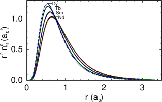
Figure 1: The spherically-symmetric 4$f$ electron density $n^{0}_{4f}(r)$ calculated for 10 compounds: NdCo₅, SmCo₅, Tb (solid lines); NdFe₁₂, SmFe₁₂ (dashed); NdFe₁₂N, SmFe₁₂N, TbFe₂, DyFe₂ (dotted); Sm₂Co₁₇ (long dash). The data fall onto four distinct curves depending on the lanthanide.

In Fig. 1 we plot $n^{0}_{4f}(r)$ obtained for each of the 10 materials in our test set (more details regarding the test set can be found in Sec. 3.1). The most notable feature of Fig. 1 is that $n^{0}_{4f}(r)$ depends on the lanthanide but not on the host compound. As a result, the 10 curves are effectively reduced to 4, corresponding to the number of lanthanides in the test set (Nd, Sm, Tb and Dy).

Physically, the observation that $n^{0}_{4f}(r)$ depends on the lanthanide but not the host compound is consistent with the picture of atomic-like 4$f$ electrons. Practically, this behaviour could be useful for studies screening a large number of candidate compounds based on their CF coefficients. To a good approximation, Fig. 1 supports the idea that one need not recalculate $n^{0}_{4f}(r)$ for every compound, but rather predefine one function for each lanthanide to be used for the full set of candidates. Then the computational work would be restricted to calculating only the potential $V_{lm}^{\sigma}(r)$ for the Y-analogues. For the current manuscript, however, we have recalculated $n^{0}_{4f}(r)$ for each compound.

2.8 “$B$” and “$A$” CF coefficients and axis orientation

Since we have chosen to expand the potential in terms of complex spherical harmonics (2), it is natural to work with the CF coefficients conventionally labelled $B$. These coefficients correspond to expanding the potential with Wybourne operators, which are related to the spherical harmonics by the prefactor appearing in (3) [41, 42]. Within this normalization one can distinguish “real” and “imaginary” CF coefficients depending on the relationship between $B_{lm}$ and $B_{l-m}$. For the materials considered here we have chosen the crystal axes such that the imaginary CF coefficients are zero, so $B_{lm}$ = $B_{l-m}$.

In the past and present CF literature it is more common to find CF coefficients $[A_{lm}\langle r^{l}\rangle]$ which are based on Stevens operators [41]. Ref. [41] gives a table of factors $\alpha_{lm}$ which allow the conversion $[A_{lm}\langle r^{l}\rangle]=\alpha_{lm}B_{lm}$ to be performed. To facilitate comparison with previous work we perform this conversion and report our results using the Stevens form. We stress that despite the notation, $[A_{lm}\langle r^{l}\rangle]$ should be considered a single quantity in our calculations (hence the square brackets) and cannot be be factored into $A_{lm}$ and $\langle r^{l}\rangle$.

We also point out an issue relevant to materials with non-orthogonal axes, e.g. hexagonal crystals. In the expansion of (2), the conventional relation between polar and cartesian co-ordinates applies, i.e. ${\bf\hat{r}}=(\sin\theta\cos\phi,\sin\theta\sin\phi,\cos\theta)$. For cubic and tetragonal crystal structures, it makes sense to choose the crystal axes to coincide with the three cartesian directions. However, for a hexagonal system with the $c$ axis pointing in the $z$ direction, one can choose a crystal axis also to point in the $x$ or $y$ direction.

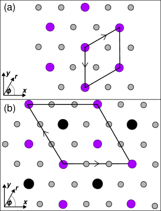
Figure 2: (a) The RECo₅ (CaCu₅) crystal structure [9], showing just the $ab$ plane containing the RE atom. The hexagonal unit cell according to the convention of Ref. [61] is shown with the cartesian axes and polar co-ordinate representation. (b) The RE₂Co₁₇ (Th₂Zn₁₇) crystal structure. Notice how the unit cell is rotated compared to (a), but the hexagonal array of Co atoms surrounding the RE are in the same orientation. Grey circles represent Co, purple RE and black represents pairs of Co atoms (dumbbells).

The reason that such a choice has an impact on CF coefficients, specifically those with nonzero $m$, is illustrated in Fig. 2(a). Here the SmCo₅ structure is shown, focusing on the $ab$ plane containing the Sm atoms. Figure 2(a) obeys the convention given in the book by Bradley and Cracknell [61], so that one of the hexagonal lattice vectors is parallel to the $-y$ direction. Such a system will in general have a nonzero $B_{66}$, which is also equal to $B_{6-6}$. However, one could construct a hexagonal co-ordinate system with a hexagonal vector parallel to the $x$ direction, corresponding to a 90^∘ rotation in the $ab$ plane. Since $Y_{6\pm 6}\propto e^{\pm 6i\phi}$, $B_{66}$ and $B_{6-6}$ would flip sign with this choice of axes. Physically, the difference occurs because in one case a vector with $\phi=0$ and its origin at the RE site points towards the nearest neighbour Co atom, while for the other case the vector points exactly between two.

In this work, we mainly follow the convention of Fig. 2(a) when dealing with hexagonal systems. The key exception is Sm₂Co₁₇, where we have a hexagonal vector pointing along the $x$ direction [Fig. 2(b)]. This choice of axes for Sm₂Co₁₇ ensures that the imaginary $B$ coefficients are zero, and actually gives a local environment for the Sm atoms which is more similar to SmCo₅ [i.e. nearest in-plane Co atoms lying close to the $\phi=0$ direction, which can be seen by comparing Figs. 2(a) and (b)].

We have drawn attention to this issue because not all codes agree on the cartesian orientation of hexagonal axes. For instance, the Hutsepot KKR code [62] used to perform the LSIC calculation uses the orientation of Fig. 2(a) for hexagonal crystals by default. However, in the Quantum Espresso package [51] or the Atomic Simulation Environment (ASE) [63] hexagonal axes are defined with a lattice vector pointing parallel to the $x$ direction [Fig. 2(b)]. With this in mind we think it useful when reporting crystal field coefficients with nonzero $m$ for hexagonal structures to also give the relationship between crystal axes and $\theta$ and $\phi$.

Finally, we note an additional potential source of confusion is that in experimental literature there are $B$ coefficients which are distinct from those introduced above. These alternative $B$ coefficients are the $[A_{lm}\langle r^{l}\rangle]$ quantities multiplied by the appropriate Stevens coefficient $\alpha_{J}$, $\beta_{J}$ or $\gamma_{J}$, depending on $l$  [64]. For clarity, we do not refer to these quantities any further here.

2.9 Anisotropy constants from crystal field coefficients

This work focuses on the calculation of CF coefficients. However, experimental studies involving magnetization measurements more commonly report anisotropy constants, which (for a uniaxial system) come from an expansion of the free energy in terms of the magnetization direction ($\theta_{0}$, $\phi_{0}$):

$$E(\theta_{0},\phi_{0}) = K_{1}\sin^{2}\theta_{0}+K_{2}\sin^{4}\theta_{0}+K_{3}\sin^{6}\theta_{0}$$ (15)

$$+K_{4}\sin^{6}\theta_{0}\cos 6\phi_{0}.$$

For Tb, where there is no contribution from the TM, we can calculate the $K_{i}$ values by diagonalizing the Hamiltonian in (1) within the ground $J$ manifold ($L$=$S$=3, $J$ = 6). We choose the magnitude of the external field in (1) to be very large (5000 T) which constrains the magnetization to point along the chosen field direction ${\bf\hat{B}}$. The zero temperature (ground state) energy is thus obtained as a function of magnetization angle, which can be fitted to the expression 15. In the case that the $l=2$ term dominates, the following relation is satisfied [42]:

$$K_{1}=-3J(J-0.5)\alpha_{J}[A_{20}\langle r^{2}\rangle].$$ (16)

For a general RE-TM magnet it is not straightforward to relate CF coefficients to the $K_{i}$ constants. This is because the CF coefficients only contain the contribution of the RE, but the TM will also contribute to the anisotropy [42]. However, making the reasonable assumption that the RE provides the dominant contribution, one can use the CF coefficients to at least make qualitative statements about the anisotropy. For instance, multiplying the signs of the Stevens factor $\alpha_{J}$ and $[A_{20}\langle r^{2}\rangle]$ gives the sign of negative $K_{1}$, assuming the $l=2$ term is dominant (16). Similarly, for cubic systems like the Laves phase compounds (where the first nonzero CF coefficient has $l=4$), the product of $[A_{40}\langle r^{4}\rangle]$ and $\beta_{J}$ will be positive for an easy [111] direction and negative for [001]. The latter behaviour can be verified by plotting the potential $B_{40}Y_{40}(\theta)+B_{4\pm 4}Y_{4\pm 4}(\theta)$ in the $\phi=0$ plane multiplied by the sign of the Stevens factor, and seeing if the result is maximal or minimal along the [001] direction.

2.10 Computational details

We calculated the potential $V_{lm}^{\sigma}(r)$ including the PAW corrections (6) for the Y-analogues of RE-TM magnets using the GPAW code, version 1.4.0 [52]. We used the latest freely available GPAW PAW datasets (version 0.9.2) [56]. The calculations were performed using a plane wave basis set, expanding the wavefunctions up to a maximum plane wave kinetic energy of 1200 eV. The reciprocal space sampling was performed using $\Gamma$-centred $k$-point meshes and converged for each material, and the Kohn-Sham states occupied according to a Fermi-Dirac distribution with a width of 0.01 eV. The exchange-correlation energy was modelled with the LSDA [28]. The PAW corrections (A) were extracted using our own Python scripts.

To calculate the spherically-symmetric 4$f$ electron density $n^{0}_{4f}(r)$ we used the Hutsepot KKR code [62] to calculate the spherically-symmetric potential at the RE site within the muffin-tin approximation. The muffin tin radii are reported in Table 1. We used the LSDA + LSIC [36] to model the XC energy, where the angular momentum channels were corrected according to the scheme described in Ref. [31]. Using this potential we solved the atomic problem on a logarithmic radial grid to obtain the Green’s function and density [(13) and (14)]. Finally, $V_{lm}^{\sigma}(r)$ and $n^{0}_{4f}(r)$ were combined to calculate CF coefficients from (4) and converted into $[A_{lm}\langle r^{l}\rangle]$ notation [41].

3 Results

3.1 Materials considered

Table 1: Structural parameters used in the calculations, with the Wyckoff positions occupied by each inequivalent atom given. Lattice parameters and muffin tin radii are in Å, internal co-ordinates of the indicated Wyckoff positions are dimensionless.

Material	Space group;	Lattice parameters;	Internal co-ordinates	Source and reference
	RE site symmetry	MT radius
SmCo5	191 (P6/mmm)	$a$ = 4.974, $c$ = 3.978	Sm(1$a$), Co(2$c$), Co(3$g$)	Exp. at 5 K [65]
	$D_{6h}$	$r_{\mathrm{MT}}$=1.645
NdCo5	191 (P6/mmm)	$a$ = 5.006, $c$ = 3.978	Nd(1$a$), Co(2$c$), Co(3$g$)	Exp. at 5 K [65]
	$D_{6h}$	$r_{\mathrm{MT}}$=1.661
Sm2Co17	166 (R$\bar{3}$m)	$a$ = 8.398, $c$ = 12.218	Sm(6$c$), Co(6$c$), Co(9$d$), Co(18$f$), Co(18$h$)	Exp. at 300 K [66]
	$C_{3v}$	$r_{\mathrm{MT}}$=1.781	$z_{6c,\mathrm{Sm}}$ = 0.343; $z_{6c,\mathrm{Co}}$ = 0.099; $x_{18f}$ = 0.283;	(Nd2Co17; see text)
			$(x,z)_{18h}$ = (0.171,0.486)
NdFe12	139 (I4/mmm)	$a$ = 8.533, $c$ = 4.681	Nd(2$a$), Fe(8$f$), Fe(8$i$), Fe(8$j$)	DFT-GGA [47]
	$D_{4h}$	$r_{\mathrm{MT}}$=1.667	$x_{8i}$ = 0.359; $x_{8j}$ = 0.268
NdFe12N	139 (I4/mmm)	$a$ = 8.521, $c$ = 4.883	Nd(2$a$), N(2$b$), Fe(8$f$), Fe(8$i$), Fe(8$j$)	DFT-GGA [47]
	$D_{4h}$	$r_{\mathrm{MT}}$=1.667	$x_{8i}$ = 0.361; $x_{8j}$ = 0.274
SmFe12	139 (I4/mmm)	$a$ = 8.497, $c$ = 4.687	Sm(2$a$), Fe(8$f$), Fe(8$i$), Fe(8$j$)	DFT-GGA [47]
	$D_{4h}$	$r_{\mathrm{MT}}$=1.667	$x_{8i}$ = 0.359; $x_{8j}$ = 0.270
SmFe12N	139 (I4/mmm)	$a$ = 8.517, $c$ = 4.844	Sm(2$a$), N(2$b$), Fe(8$f$), Fe(8$i$), Fe(8$j$)	DFT-GGA [47]
	$D_{4h}$	$r_{\mathrm{MT}}$=1.667	$x_{8i}$ = 0.361; $x_{8j}$ = 0.274
TbFe2	227 (Fd$\bar{3}$m); $T_{d}$	$a$ = 7.341, $r_{\mathrm{MT}}$=1.589	Tb(8$b$), Fe(16$c$)	Exp. at 300 K [65]
DyFe2	227 (Fd$\bar{3}$m); $T_{d}$	$a$ = 7.338, $r_{\mathrm{MT}}$=1.589	Dy(8$b$), Fe(16$c$)	Exp. at 300 K [65]
Tb	194 (P63/mmc)	$a$ = 3.606, $c$ = 5.698	Tb(2$c$)	Exp. at 300 K [67]
	$D_{3h}$	$r_{\mathrm{MT}}$=1.764

In Table 1 we list the 10 materials considered in this work. In our set of materials we have included the archetypal Sm-Co magnets SmCo₅ [7] and Sm₂Co₁₇ [8], and also examples of the 1:12 magnet class e.g. NdFe₁₂N, which are currently the subject of research due to their potential as hard magnetic materials with reduced RE content [68]. We have also included the Laves phase magnets TbFe₂ and DyFe₂ whose alloy is the highly magnetostrictive Terfenol-D compound [69, 70], and also elemental Tb [71]. Tb is an interesting test since the Y-analogue has no atoms in common with the original structure.

Table 1 also gives the structural parameters (lattice constants and internal co-ordinates) used in the calculations. In order to be able to best compare our CF coefficients to previous calculations we have where possible used the same structural parameters. Accordingly, as indicated in Table 1 structural parameters have been sourced both from experimental and computational works. For Sm₂Co₁₇ we follow Ref. [46] and use the structural parameters of the related compound Nd₂Co₁₇ [66], which avoids the experimental difficulties associated with performing neutron experiments on Sm compounds.

As clearly explained in Ref. [42], depending on the point symmetry of the RE site only certain CF coefficients will be nonzero. Furthermore, for the purposes of calculating matrix elements for $f$ electrons we need only calculate CF coefficients for even values of $l$, up to a maximum $l=6$. In order to check that our computational method is robust we calculated the decomposition of the potential (6) for all $lm$ combinations and confirmed that the only nonzero terms were those expected from the point symmetry [61].

3.2 CF coefficients

Table 2: Calculated crystal field coefficients, in K (i.e. $[A_{lm}\langle r^{l}\rangle]/k_{B}$). The two numbers reported for each $lm$ combination corresponds to spin up/down respectively, and the bold number corresponds to the spin of the asymmetric 4$f$ electron cloud, as discussed in the text.

Material	$[A_{20}\langle r^{2}\rangle]$	$[A_{40}\langle r^{4}\rangle]$	$[A_{43}\langle r^{4}\rangle]$	$[A_{44}\langle r^{4}\rangle]$	$[A_{60}\langle r^{6}\rangle]$	$[A_{63}\langle r^{6}\rangle]$	$[A_{64}\langle r^{6}\rangle]$	$[A_{66}\langle r^{6}\rangle]$
SmCo5	-402/-400	-30/-22	—	—	5/4	—	—	-137/-115
DMFT [20]	-313/-262	-40/-55	—	—	35/25	—	—	-731/-593
NdCo5	-421/-415	-36/-26	—	—	6/5	—	—	-174/-146
Sm2Co17	-199/-208	-20/-7	116/108	—	-1/-1	-22/-25	—	-54/-48
open core [46]	-194	-15	74	—	-2	-61	—	-139
NdFe12	-116/-110	4/15	—	-205/-145	10/7	—	-29/-21	—
open core [47]	-77	—	—	—	—	—	—	—
DMFT [20]	-71/-116	-5/-1	—	-76/-270	62/54	—	-224/-107	—
NdFe12N	188/364	-62/-13	—	-161/-101	-17/-16	—	-1/-3	—
open core [47]	367	—	—	—	—	—	—	—
DMFT [20]	477/653	75/112	—	-105 /-141	32/63	—	-65/-91	—
SmFe12	-100/-96	1/10	—	-154/-112	8/6	—	-21/-15	—
open core [47]	-47	—	—	—	—	—	—	—
DMFT [20]	-184/-211	-21/-18	—	-41 /-136	45/40	—	-95/-58	—
SmFe12N	272/414	-47/-6	—	-121/-75	-14/-13	—	-2/-3	—
open core [47]	371	—	—	—	—	—	—	—
DMFT [20]	195/225	78/70	—	22/-91	47/25	—	-97/-82	—
TbFe2	—	28/29	—	139/143	-2/-2	—	39/38	—
DyFe2	—	26/26	—	128/132	-2/-2	—	34/32	—
Tb	-59/-60	-4/-3	—	—	4/4	—	—	36/36

Table 2 gives the CF coefficients calculated for our set of materials. We also reproduce the values of CF coefficients calculated previously in the literature for some of the materials [20, 46, 47].

For our calculations, and Ref. [20], two numbers are reported for each $lm$, corresponding to the CF coefficient calculated using $V_{lm}^{\uparrow}(r)$ and $V_{lm}^{\downarrow}(r)$. One of the two numbers has been written in bold, corresponding to the coefficient that (in the zero temperature, scalar-relativistic picture) is the potential felt by the partially filled 4$f$ spin subshell. Expanding on this point, we first note that we have chosen the TM spins to point in the $\uparrow$ direction. Furthermore, the RE-TM coupling is generally antiferromagnetic between spins [5]. Therefore, for the light REs Nd and Sm the partially filled 4$f$ subshell has $\downarrow$ spin character, so the relevant CF coefficient is calculated using $V_{lm}^{\downarrow}(r)$. For the heavy REs, the 4$f$ $\downarrow$ spin subshell is filled, so $V_{lm}^{\uparrow}(r)$ is relevant for TbFe₂ and DyFe₂. For elemental Tb we chose $\uparrow$ to be the majority spin direction, so the unfilled 4$f$ spin subshell is $\downarrow$. We note that, except for NdFe₁₂N and SmFe₁₂N, we calculate the difference between $V_{lm}^{\uparrow}(r)$ and $V_{lm}^{\downarrow}(r)$ to be rather small. We now discuss each material in more detail.

3.2.1 SmCo₅ and NdCo₅

SmCo₅ crystallizes in the CaCu₅ structure, which is hexagonal with one formula unit in the unit cell [9]. SmCo₅ is characterized by a large uniaxial anisotropy [72], which is understood in terms of CF theory based on the approximate relation (16) between the first anisotropy constant and lowest order CF coefficient, $K_{1}\propto-\alpha_{J}[A_{20}\langle r^{2}\rangle]$ [42]. The positive value of 13/315 for the Stevens $\alpha_{J}$ coefficient of Sm³⁺ [42] means that SmCo₅ should have a large, negative value of $[A_{20}\langle r^{2}\rangle]$ [73].

Recently, Ref. [20] calculated the CF coefficients of SmCo₅ within DMFT, and also provided a useful summary of past calculations and experimental measurements. Experimentally measured values of $[A_{20}\langle r^{2}\rangle]$ vary between -180 and -420 K, whilst calculations found values between -160 and -755 K. There is no particular consensus about the other CF coefficients, although the computational works agreed in finding $[A_{40}\langle r^{4}\rangle]$ to be negative and $[A_{60}\langle r^{6}\rangle]$ to be positive. We reproduce the results of the DMFT calculations with our own results in Table 2.

Our calculations based on the Y-analogue model of SmCo₅ find values of the $[A_{20}\langle r^{2}\rangle]$ coefficient (-402/-400 K) which fall into the previously reported experimental/calculated ranges. The variation in sign of $[A_{20}\langle r^{2}\rangle]$, $[A_{40}\langle r^{4}\rangle]$ and $[A_{60}\langle r^{6}\rangle]$ also follows that observed in previous calculations. Despite the different methodologies involved, our calculated values are reasonably close to the DMFT results [20], with the exception of $[A_{66}\langle r^{6}\rangle]$. This CF coefficient controls the basal plane anisotropy. However, it does not affect the ground-$J$ multiplet of Sm [42]. Furthermore, higher order CF coefficients decay more quickly with temperature [42]. Therefore, the effect of $[A_{66}\langle r^{6}\rangle]$ on the strongly uniaxial SmCo₅ is expected to be difficult to observe, and has not been measured experimentally [73].

For comparison we also considered the isostructural NdCo₅ compound. Within the Y-analogue model, any differences between CF coefficients calculated for SmCo₅ and NdCo₅ must be attributed to (a) the slightly different lattice parameters (Table 1) and (b) the different 4$f$ electron density (Fig. 1). We see from Table 2 that the calculated CF coefficients are actually very similar for both materials. However, Nd³⁺ has a negative Stevens factor (-7/1089) [42], which means NdCo₅ should have an in-plane anisotropy (negative $K_{1}$), This is exactly what is observed experimentally [74]. Furthermore, unlike SmCo₅ the anisotropy within the basal plane has also been measured experimentally, with the easy direction found to point between Co atoms [64] [$\phi=30^{\circ}$ in Fig. 2(a)]. This easy direction is indeed consistent with the negative $[A_{66}\langle r^{6}\rangle]$ which we calculate, since the Stevens $\gamma_{J}$ ($l$=6) coefficient of Nd³⁺ is negative [42].

3.2.2 Sm₂Co₁₇

The magnet Sm₂Co₁₇ forms in the Th₂Zn₁₇ structure. This structure is closely related to SmCo₅ by an ordered substitution of one in three Sm atoms with a pair (dumbbell) of Co atoms [9]. Although there is a distortion of the local environment, the Sm atoms are still surrounded by a hexagon of effectively coplanar Co atoms, as shown in Fig. 2(b). However, as is also clear from Fig. 2(b) the dumbbells lower the hexagonal symmetry so that CF coefficients with $m=\pm 3$ are nonzero. What is not shown in Fig. 2 is the tripling of the unit cell along the $c$ direction compared to SmCo₅, due to the stacking of two Sm atoms and a dumbbell. Again we stress that our choice of axes in Fig. 2(b) is unconventional compared to Fig. 2(a), but physically gives a closer correspondence between the $(\theta,\phi)$ co-ordinate system and the positions of atoms in SmCo₅.

Now considering the calculated $[A_{lm}\langle r^{l}\rangle]$ in Table 2, we see that introducing the Co dumbbells results in reduced coefficients compared to SmCo₅. In particular, $[A_{20}\langle r^{2}\rangle]$ is halved. The value of -208 K is still negative however, supporting uniaxial anisotropy as is observed experimentally [9]. In terms of anisotropy within the basal plane, $[A_{66}\langle r^{6}\rangle]$ is negative like in SmCo₅, but is weaker by a factor of 2.

Ref. [46] reported calculations of the CF coefficients of Sm₂Co₁₇, modelling the Sm in the 3+ state with the open-core approximation. We reproduce the calculated values in Table 2, and find very close agreement with our Y-analogue model. The exception is for the $l=6$ coefficients, with Ref. [46] finding values a factor of 3 larger than our calculations. As for SmCo₅, there is no experimental data for these coefficients. However, we think that it is reasonable that our calculations show a reduction in $[A_{66}\langle r^{6}\rangle]$ for Sm₂Co₁₇ compared to SmCo₅, due to the disrupted hexagonal symmetry.

3.2.3 NdFe₁₂, NdFe₁₂N, SmFe₁₂, SmFe₁₂N

Members of the 1:12 magnet class have a tetragonal, ThMn₁₂ crystal structure with the RE surrounded by 3 TM sublattices. The interstitial $2b$ positions can also be occupied by nonmetal atoms, forming e.g. NdFe₁₂N [68]. The fourfold symmetry in the $ab$ plane gives rise to nonzero CF coefficients with $m\pm 4$. However, it is the lowest order coefficient $[A_{20}\langle r^{2}\rangle]$ (which decays the slowest with temperature) which is expected to have the largest effect on the uniaxial anisotropy. As for the materials above, a negative value of $[A_{20}\langle r^{2}\rangle]$ is expected to yield uniaxial anisotropy for Sm and planar anisotropy for Nd, based on the sign of the Stevens coefficient.

Table 2 shows our calculated CF coefficients for NdFe₁₂, NdFe₁₂N, SmFe₁₂ and SmFe₁₂N. The most striking feature is the sign reversal of $[A_{20}\langle r^{2}\rangle]$ upon nitrogenation, switching from negative to positive. These signs mean that SmFe₁₂ and NdFe₁₂N should have uniaxial anisotropy, and NdFe₁₂ and SmFe₁₂N should be planar. Nitrogenation also provides a negative contribution to $[A_{40}\langle r^{4}\rangle]$, but weakens $[A_{44}\langle r^{4}\rangle]$. The $l=6$ CF coefficents are small for all of the materials.

Also in Table 2 we reproduce reported CF coefficients calculated with DMFT [20] and with the open core approximation [47] (only the $l$=2 coefficients are reported in Ref. [47]). Focusing first on $[A_{20}\langle r^{2}\rangle]$ we find that the three methods calculate the same signs. Furthermore there is close numerical agreement between our Y-analogue calculations and the open core calculations [47], as for Sm₂Co₁₇. However, there is no systematic level of agreement of these calculations with DMFT, with for instance similar values calculated for NdFe₁₂ but variations up to a factor of two for the other materials. The agreement between the Y-analogue model and DMFT for the higher order CF coefficients is similarly unsystematic, with for instance opposite signs found for $[A_{40}\langle r^{4}\rangle]$ but quite close agreement for $[A_{44}\langle r^{4}\rangle]$. Like for SmCo₅, the DMFT calculations find larger values of $l$=6 coefficients than in the Y-analogue model.

We note that both the DMFT and Y-analogue calculations find that nitrogenation introduces a significant difference between the $\uparrow$ and $\downarrow$ CF coefficients. At first sight, this observation is puzzling since N is nonmagnetic. However, as shown in Ref. [47] the introduction of N strengthens the magnetization by approximately 2.5 $\mu_{\mathrm{B}}$ per formula unit, which our calculations find is due to an enhanced Fe magnetization at the 8$f$ sites. The 8$f$ sites sit halfway between RE planes, so it is not unreasonable that an enhanced spin polarization here will affect the $\uparrow$ and $\downarrow$ CF coefficients by differing amounts.

Finally, comparing the Y-analogue calculations between Nd and Sm compounds we see that the same qualitative behavior of the CF coefficients is observed. However, unlike for SmCo₅ and NdCo₅ there are some numerical differences, particularly for the nitrided compounds where there is a large difference in $c$ parameter for NdFe₁₂N and SmFe₁₂N.

3.2.4 TbFe₂ and DyFe₂

The Laves phase REFe₂ compounds are notable for their large room temperature magnetostrictions, particularly the alloy Tb_0.27Dy_0.73Fe₂ (Terfenol-D) [69, 70]. Unlike the other materials in our test set the Laves phase (MgCu₂) structure is cubic, yielding a zero $[A_{20}\langle r^{2}\rangle]$ coefficient. They are also key examples of RE-TM magnets based on heavy REs with practical applications.

In Table 2 we give the CF coefficients calculated using the Y-analogue model for TbFe₂ and DyFe₂. We point out that although four coefficients are presented for each material, only $[A_{40}\langle r^{4}\rangle]$ and $[A_{60}\langle r^{6}\rangle]$ are independent, with the cubic symmetry fixing the ratios $B_{44}:B_{40}$ and $B_{64}:B_{60}$ [61]. The first notable feature is that the calculated coefficients are almost identical for TbFe₂ and DyFe₂. As a consequence, within CF theory any different behavior of the anisotropy must come from the Stevens factors.

The $\beta_{J}$ ($l$=4) factors are 2/16335 and -8/135135 for Tb³⁺ and Dy³⁺, respectively. The $\gamma_{J}$ coefficients also have opposite signs [42]. Therefore, one would expect TbFe₂ and DyFe₂ to have different easy directions of magnetization, either [111] or [100]. Specifically, based on the positive $l=4$ CF coefficients one would expect an easy direction of [111] for TbFe₂ and [100] for DyFe₂ (Sec. 2.9). This behaviour is exactly what is observed experimentally; indeed the easy directions of all of the heavy RFe₂ compounds follow the sign of $\beta_{J}$ [65].

To our knowledge the CF coefficients of TbFe₂ and DyFe₂ have not been calculated from first principles previously. Experimental determination of these cubic terms is also expected to be difficult due to the large magnetostrictive effect. For example, based on Mössbauer measurements the authors of Ref. [75] were unable to determine precise values of $[A_{lm}\langle r^{l}\rangle]$, except that $A_{40}$ was of order 10 K/$a_{0}^{4}$. Furthermore, the ratio $A_{60}/A_{40}$ was determined to be -0.04$a_{0}^{-2}$. As pointed out in Sec. 2.8, we cannot extract $A_{lm}$ from $\langle r^{l}\rangle$ so a direct comparison is not possible. However, our value of $[A_{40}\langle r^{4}\rangle]$ is also of order 10 K, and our calculated ratio $[A_{60}\langle r^{6}\rangle]/[A_{40}\langle r^{4}\rangle]$ is -0.08. Therefore we can at least say that the sign of the ratio of the $l$ = 4 and 6 CF coefficients is consistent with Ref. [75], and also that the magnitudes are reasonable.

3.2.5 Tb

The final material we consider is elemental Tb. Here, every atom in the system is replaced with Y, so arguably this material presents the most difficult challenge to the Y-analogue model, even though the nominal valence electron configurations are the same.

Tb is hexagonal, and has the same nonzero CF coefficients as NdCo₅. Indeed, as seen in Table 2 the relative magnitudes of the different CF coefficients of Tb follow those of NdCo₅ reasonably closely, except for the crucial difference of $[A_{66}\langle r^{6}\rangle]$, which is positive for Tb. Noting that Tb³⁺ has negative Stevens $\alpha_{J}$ and $\gamma_{J}$ coefficients like Nd³⁺, the calculated CF coefficients lead to easy plane anisotropy, with a preferred direction in the basal plane of $\phi=0$, i.e. pointing between the nearest in-plane Tb atoms [Fig. 2(a)]. The calculated easy direction matches that observed experimentally [64].

Unlike the other materials in our test set, there are no other magnetic sublattices present in Tb. Therefore, we can use the method described in Sec. 2.9 to calculate anisotropy constants at 0 K, obtaining values of -17, -12 and 5 MJm^-3 for $K_{1}$, $K_{2}$ and $K_{3}$, and -0.2 MJm^-3 for $K_{4}$. These numbers are smaller than the values reported from low temperature high-field measurements, e.g. -60 MJm^-3 for $K_{1}$ only, and -2.4 MJ for $K_{4}$ [71, 76]. However it is important to remember that our calculations do not include magnetostrictive effects, which are highly important in Tb. For instance, the high-field magnetization curve clearly shows a hysteresis, which has been attributed to a plastic deformation of the crystal [76].

4 Conclusions and outlook

Aside from the numerical results of our work contained in Table 2, we can summarize our results qualitatively as follows:

• The signs of our calculated CF coefficients are consistent with experimentally-observed/previously calculated magnetization directions for all 10 materials (easy axis: SmCo₅, Sm₂Co₁₇, NdFe₁₂N, SmFe₁₂; easy plane: NdCo₅, NdFe₁₂, SmFe₁₂N, Tb; [111] axis: TbFe₂; [001] axis, DyFe₂).

• For systems with data available (NdCo₅ and Tb), the signs of the $[A_{66}\langle r^{6}\rangle]$ coefficients are also consistent with the experimentally-observed basal plane anisotropy.

• Our calculated CF coefficients are generally close (within 50 K/4 meV) of previously reported open core calculations.

• The trend across the Sm-Co series behaves intuitively, with CF coefficients weakened for lower symmetry (SmCo₅ vs Sm₂Co₁₇).

Taken together, our results demonstrate that the Y-analogue model is a viable method of calculating CF coefficients of RE-TM magnets. Of course, it is not the only method, and we do not claim that it is any more accurate than previously published work [12, 17, 20, 44, 45, 46, 47, 48]. In our opinion the strength of the Y-analogue model is in the simplicity of the calculation of the CF potential $V({\bf r})$. Whilst implemented in some DFT codes like OpenMX [77], the open-core approximation (which appears to give similar CF coefficients to the Y-analogue model), is not yet universally available. By contrast, the PAW dataset for Y is distributed as standard in all of the popular DFT codes. We also find the calculations involving Y to be numerically stable. As such, we would expect a high degree of reproducibility of the CF potential calculated for Y-analogues using different codes, similar to that demonstrated e.g. for bulk moduli [78].

As noted in Sec. 2, the CF potential must be supplemented by the radial 4$f$ charge density $n^{0}_{4f}(r)$ in order to calculate the CF coefficient. Unfortunately, calculating $n^{0}_{4f}(r)$ is not completely straightforward, requiring a way of dealing with the 4$f$ electrons like the LSIC. However, as we argued in the discussion surrounding Fig. 1, the same $n^{0}_{4f}(r)$ could be used to calculate the CF coefficients for a range of compounds containing a given lanthanide. This further approximation would then mean only the CF potential needed to be calculated for each compound, enabling high throughput computational screening of materials based on their calculated CF coefficients and scaling up the work of e.g. Refs. [19, 26].

From the point of view of assessing the predictive power of our calculations, the most interesting avenue for future exploration is to go beyond calculating CF coefficients and instead target quantities that can be directly compared to experiments, e.g. magnetization versus field curves, from which anisotropy constants $K_{i}$ (15) are extracted. Although we tentatively discussed anisotropy constants for Tb, our ability to compare to experiment was limited due to us not taking any magnetoelastic effects into account. Including such effects will be crucial if we are to properly account for the magnetostriction of the heavy RE materials, including elemental Tb [71, 76] and the Laves phase Tb_1-xDy_xFe₂ compounds [69].

More generally, we did not attempt to determine $K_{i}$ for the RE-TM compounds here since the CF coefficients do not include the contribution to the anisotropy from the TM. However, we have previously calculated the TM contribution for GdCo₅ (which has no crystal field effects) and obtained values of $K_{i}$ in quantitative agreement with experiment, over a range of temperatures [79]. Therefore, by combining the method presented here with our previous work [79] and finite temperature CF theory [42], we should have the necessary tools to calculate temperature-dependent anisotropy constants of RE-TM magnets entirely from first principles.

Appendix A Explicit expression for correction to the pseudo-density

Here we give the explicit expression for the angular expansion of the correction to the pseudo-density. We use standard GPAW notation [52]. The difference between the full and pseudized density $\Delta\rho({\bf r})$ is the sum of the electronic contribution $\Delta n({\bf r})$ and a nuclear part:

$$\Delta\rho({\bf r})=\Delta n({\bf r})-Z\delta({\bf r})-\sum_{lm}Q_{lm}g_{lm}({\bf r})$$ (17)

Here, $Z$ is the nuclear charge (a positive number), $Q_{lm}$ are the compensation charges used to ensure the multipole moments of $\Delta\rho({\bf r})$ are zero, and $g_{lm}$ are functions which in GPAW are Gaussians multiplied by real spherical harmonics. The spin-resolved correction for the electronic density is

$$\Delta n^{\sigma}({\bf r}) = \frac{n_{c}(r)-\tilde{n}_{c}(r)}{2}+$$ (18)

$$\sum_{i_{1}i_{2}}D_{\sigma i_{1}i_{2}}[\phi_{i_{1}}({\bf r})\phi_{i_{2}}({\bf r})-\tilde{\phi}_{i_{1}}({\bf r})\tilde{\phi}_{i_{2}}({\bf r})].$$

Here, $n_{c}$ and $\tilde{n}_{c}$ are the full and pseudo core densities. $D$ is the atomic density matrix and $\phi$, $\tilde{\phi}$ are the partial waves, which together allow the reconstruction of the wavefunction in the rapidly-varying region close to the nucleus. $i$ is a composite index standing for ($\nu,l,m$) where $\nu$ plays the role of the principal quantum number of the partial waves.

$Z$, $g_{lm}$, $n_{c}$, $\tilde{n}_{c}$, $\phi$ and $\tilde{\phi}$ are properties of the PAW dataset, while $Q_{lm}$ and $D_{\sigma i_{1}i_{2}}$ are determined in the self-consistent calculation. Noting that the compensation charges and the partial waves have the forms $g_{lm}({\bf r})=g_{l}(r)Y^{R}_{lm}({\bf\hat{r}})$ and $\phi_{i_{1}}({\bf r})=\phi_{\nu l}(r)Y^{R}_{lm}({\bf\hat{r}})$ respectively, with the $R$ denoting real spherical harmonics, the angular expansions of $\Delta\rho$ and $\Delta n^{\sigma}$ are readily obtained. The only slight complication is the use of real spherical harmonics in GPAW, which means that one must take some care with integrals like $\int d{\bf\hat{r}}Y^{*}_{lm}({\bf\hat{r}})Y^{R}_{l^{\prime}m^{\prime}}({\bf\hat{r}})$ and $\int d{\bf\hat{r}}Y^{*}_{lm}({\bf\hat{r}})Y^{R}_{l_{1}m_{1}}({\bf\hat{r}})Y^{R}_{l_{2}m_{2}}({\bf\hat{r}})$.

References

References

- [1] Hirosawa S 2018 Scr. Mater. 154 245
- [2] Gutfleisch O, Willard M A, Brück E, Chen C H, Sankar S G and Liu J P 2011 Adv. Mater. 23 821
- [3] Coey J M D 2011 IEEE Trans. Magn. 47 4671
- [4] Gignoux D and Schmitt D 1995 Chapter 138 magnetic properties of intermetallic compounds (Handbook on the Physics and Chemistry of Rare Earths vol 20) pp 293 – 424
- [5] Brooks M S S, Eriksson O and Johansson B 1989 J. Phys. Condens. Matter 1 5861
- [6] Buschow K H J 1977 Rep. Prog. Phys. 40 1179
- [7] Strnat K, Hoffer G, Olson J, Ostertag W and Becker J J 1967 J. Appl. Phys. 38 1001
- [8] Strnat K 1972 IEEE Trans. Magn. 8 511
- [9] Kumar K 1988 J. Appl. Phys. 63 R13
- [10] Sagawa M, Fujimura S, Togawa N, Yamamoto H and Matsuura Y 1984 J. Appl. Phys. 55 2083
- [11] Croat J J, Herbst J F, Lee R W and Pinkerton F E 1984 J. Appl. Phys. 55 2078
- [12] Richter M 1998 J. Phys. D: Appl. Phys. 31 1017
- [13] Larson P, Mazin I I and Papaconstantopoulos D A 2003 Phys. Rev. B 67 214405
- [14] Kashyap A, Skomski R, Sabiryanov R F, Jaswal S S and Sellmyer D J 2003 IEEE Trans. Magn. 39 2908
- [15] Miura Y, Tsuchiura H and Yoshioka T 2014 J. Appl. Phys. 115 17A765
- [16] Matsumoto M, Banerjee R and Staunton J B 2014 Phys. Rev. B 90 054421
- [17] Miyake T, Terakura K, Harashima Y, Kino H and Ishibashi S 2014 J. Phys. Soc. Jpn. 83 043702
- [18] Harashima Y, Terakura K, Kino H, Ishibashi S and Miyake T 2015 Phys. Rev. B 92 184426
- [19] Körner W, Krugel G and Elsässer C 2016 Sci. Rep. 6 24686
- [20] Delange P, Biermann S, Miyake T and Pourovskii L 2017 Phys. Rev. B 96 155132
- [21] Chouhan R K and Paudyal D 2017 J. Alloys Compd 723 208
- [22] Patrick C E, Kumar S, Balakrishnan G, Edwards R S, Lees M R, Mendive-Tapia E, Petit L and Staunton J B 2017 Phys. Rev. Mater. 1 024411
- [23] Toga Y, Nishino M, Miyashita S, Miyake T and Sakuma A 2018 Phys. Rev. B 98 054418
- [24] Sakurai M, Wu S, Zhao X, Nguyen M C, Wang C Z, Ho K M and Chelikowsky J R 2018 Phys. Rev. Mater. 2 084410
- [25] Miyake T and Akai H 2018 J. Phys. Soc. Jpn. 87 041009
- [26] Tatetsu Y, Harashima Y, Miyake T and Gohda Y 2018 Phys. Rev. Mater. 2 074410
- [27] Kohn W and Sham L J 1965 Phys. Rev. 140 A1133
- [28] Vosko S H, Wilk L and Nusair M 1980 Can. J. Phys. 58 1200
- [29] Perdew J P, Burke K and Ernzerhof M 1996 Phys. Rev. Lett. 77 3865
- [30] Richter M and Eschrig H 1991 Physica B: Condens. Matter 172 85
- [31] Patrick C E and Staunton J B 2018 Phys. Rev. B 97 224415
- [32] Brooks M S S, Nordstrom L and Johansson B 1991 J. Phys. Condens. Matter 3 2357
- [33] Kotliar G, Savrasov S Y, Haule K, Oudovenko V S, Parcollet O and Marianetti C A 2006 Rev. Mod. Phys. 78 865
- [34] Perdew J P and Zunger A 1981 Phys. Rev. B 23 5048
- [35] Anisimov V I, Aryasetiawan F and Lichtenstein A I 1997 J. Phys. Condens. Matter 9 767
- [36] Lüders M, Ernst A, Däne M, Szotek Z, Svane A, Ködderitzsch D, Hergert W, Györffy B L and Temmerman W M 2005 Phys. Rev. B 71 205109
- [37] Györffy B L, Pindor A J, Staunton J, Stocks G M and Winter H 1985 J. Phys. F: Met. Phys. 15 1337
- [38] Hummler K and Fähnle M 1996 Phys. Rev. B 53 3272
- [39] Bleaney B and Stevens K W H 1953 Rep. Prog. Phys. 16 108
- [40] Griffith J S 1961 The theory of transition-metal ions (Cambridge University Press)
- [41] Newman D J and Ng B 1989 Rep. Prog. Phys. 52 699
- [42] Kuz’min M D and Tishin A M 2008 vol 17 (Elsevier B.V.) chap 3, p 149
- [43] Tie-song Z, Han-min J, Guang-hua G, Xiu-feng H and Hong C 1991 Phys. Rev. B 43 8593
- [44] Richter M, Steinbeck L, Nitzsche U, Oppeneer P M and Eschrig H 1995 J. Alloys Compd 225 469
- [45] Novák P 1996 Phys. Status Solidi B 198 729–740
- [46] Steinbeck L, Richter M, Nitzsche U and Eschrig H 1996 Phys. Rev. B 53 7111
- [47] Harashima Y, Terakura K, Kino H, Ishibashi S and Miyake T 2015 Proceedings of Computational Science Workshop 2014 (CSW2014) p 011021
- [48] Novák P, Knížek K and Kuneš J 2013 Phys. Rev. B 87 205139
- [49] Buck S and Fähnle M 1997 J. Magn. Magn. Mater. 166 297
- [50] Blöchl P E 1994 Phys. Rev. B 50 17953
- [51] Giannozzi P et al. 2009 J. Phys. Condens. Matter 21 395502
- [52] Enkovaara J et al. 2010 J. Phys. Condens. Matter 22 253202
- [53] Kresse G and Joubert D 1999 Phys. Rev. B 59 1758
- [54] Stevens K W H 1952 Proc. Phys. Soc. 65 209
- [55] Martin R M 2004 Electronic Structure: Basic theory and practical methods (Cambridge University Press)
- [56] Information regarding the PAW datasets may be found at https://wiki.fysik.dtu.dk/gpaw/setups/setups.html
- [57] Lebedev V and Laikov D 1999 Dokl. Math. 59 477
- [58] Györffy B L and Stocks G M 1979 Electrons in Disordered Metals and at Metallic Surfaces (Springer US) chap 4, pp 89–192 Nato Science Series B
- [59] Ebert H, Ködderitzsch D and Minár J 2011 Rep. Prog. Phys. 74 096501
- [60] Tamura E 1992 Phys. Rev. B 45 3271
- [61] Bradley C J and Cracknell A P 1972 The Mathematical Theory of Symmetry in Solids (Oxford University Press)
- [62] Däne M, Lüders M, Ernst A, Ködderitzsch D, Temmerman W M, Szotek Z and Hergert W 2009 J. Phys. Condens. Matter 21 045604
- [63] Larsen A H et al. 2017 J. Phys.: Condens. Matter 29 273002
- [64] Radwański R J 1987 J. Phys. F: Met. Phys. 17 267
- [65] Andreev A V 1995 Handbook of Magnetic Materials vol 8 (Elsevier North-Holland, New York) chap 2, p 59
- [66] Herbst J F, Croat J J, Lee R W and Yelon W B 1982 J. Appl. Phys. 53 250–256
- [67] Smidt F and Daane A 1963 J. Phys. Chem. Solids 24 361
- [68] Gabay A and Hadjipanayis G 2018 Scr. Mater. 154 284
- [69] Clark A E 1973 Appl. Phys. Lett. 23 642
- [70] Abbundi R and Clark A 1977 IEEE Trans. Magn. 13 1519
- [71] Rhyne J J and Clark A E 1967 J. Appl. Phys 38 1379
- [72] Ermolenko A 1976 IEEE Trans. Magn. 12 992
- [73] Buschow K, van Diepen A and de Wijn H 1974 Solid State Commun. 15 903
- [74] Klein H, Menth A and Perkins R 1975 Physica (Amsterdam) 80B+C 153
- [75] Atzmony U, Dariel M P, Bauminger E R, Lebenbaum D, Nowik I and Ofer S 1973 Phys. Rev. B 7 4220
- [76] Chikazumi S, Tanuma S, Oguro I, Ono F and Tajima K 1969 IEEE Trans. Magn. 5 265–268
- [77] Ozaki T 2003 Phys. Rev. B 67 155108
- [78] Lejaeghere K et al. 2016 Science 351
- [79] Patrick C E, Kumar S, Balakrishnan G, Edwards R S, Lees M R, Petit L and Staunton J B 2018 Phys. Rev. Lett. 120 097202