Dynamic importance of network nodes is poorly predicted by static structural features

Abstract

One of the most central questions in network science is: which nodes are most important? Often this question is answered using structural properties such as high connectedness or centrality in the network. However, static structural connectedness does not necessarily translate to dynamical importance. To demonstrate this, we simulate the kinetic Ising spin model on generated networks and one real-world weighted network. The dynamic impact of nodes is assessed by causally intervening on node state probabilities and measuring the effect on the systemic dynamics. The results show that structural features such as network centrality or connectedness are actually poor predictors of the dynamical impact of a node on the rest of the network. A solution is offered in the form of an information theoretical measure named integrated mutual information. The metric is able to accurately predict the dynamically most important node (“driver” node) in networks based on observational data of non-intervened dynamics. We conclude that the driver node(s) in networks are not necessarily the most well-connected or central nodes. Indeed, the common assumption of network structural features being proportional to dynamical importance is false. Consequently, great care should be taken when deriving dynamical importance from network data alone. These results highlight the need for novel inference methods that take both structure and dynamics into account.

1 Introduction

Understanding complex systems is a fundamental problem for the 21st century [23]. Despite the apparent differences and purposes of many real-world networked complex systems, previous research shows several universal characteristics in networks properties such as the small-world phenomenon [57], fat-tail degree [39], and feedback loops [53]. This has lead to the common but often implicit assumption that the connectedness of a node in the network is proportional to its dynamic importance [24]. For example in epidemic research, high degree nodes or “super-spreaders” are associated to dominant epidemic risk and therefore deserve special attention [49]. Yet, prior research shows that the shared network characteristics is not shared in the dynamic or functional properties that are exerted on these networks [3, 20]. In particular, the dynamic importance of a node varies as a function of both the dynamics that exist on the network in addition to its structural connectedness. This effect was rigorously shown by Harush and colleagues [20]. In their study, the dynamic processes were varied while keeping the network structure the same. Both random generated networks as well as real-world networks were studied. Nodal importance was computed based on the “information flow” through a node. The flow through a node had a non-linear relation between its structural connectedness and the type of dynamics present in the system. These results highlight the non-intuitive and non-trivial interplay of the structure of a system and dynamics between the nodes of a system. However, the results required full knowledge of the system, i.e. both the network structure and the dynamics of the system are required to estimate the node with the highest dynamic importance. For a real-world system having both the dynamics available and the underlying network structure may be difficult. In addition, in their study the network structure was deemed constant. It remains unclear whether the proposed flow would generalize to systems with varying network structure. In addition, the results were obtained from steady-state. For dynamical processes an out-of-equilibrium approach highlight how trajectories generate systemic behavior. What is needed are methods that can detect the highest dynamic importance of a node from observations directly without knowing or assuming the underlying network or causal structure among variables.

A node’s dynamic (or causal) importance, is traditionally inferred by means of interventions and counterfactuals [40, 59]. Through external interventions the behavior of the system may change. That is, an intervention on a part of the system causes a divergence of the system behavior proportional to its dynamic importance; high causal importance relates to a large change in the system behavior. It is common for studies using causal interventions apply so-called hard intervention strategies [46]. In hard interventions a node is pinned to a state. This effectively removes all incoming connections to a node, removing all influences the system has on this node. The use of hard interventions is common in various disciplines such as gene-knockout experiments, epidemic spreading, network analysis and driver node identification.

Applying external interventions to identify nodes with high dynamical importance, referred to as driver nodes, is challenging for three reasons. First, hard interventions may cause a change in systemic behavior that does not occur in the non-intervened behavior (e.g. see fig. 1 B ) or may be impossible in practice (e.g. requiring infinite resources [56]). This complicates theory forming on what mechanisms underlie observed systemic behavior. Second, most approaches for causal inference assume that the causal interactions follow a particular structure without (local) loops [35, 14, 9]. This assumption simplifies theoretical analysis and is in many cases justified under the assumption that causes precede their effects in time. However, this approach assumes that the underlying causal structure is known and or accessible. If the underlying causal structure is not known, it has to be inferred from data which prompts problems in terms of temporal resolution and scale. For example in a causal process where $A\to B\to C\to A$, the cycle may be unrolled over time. This effectively removes cycles. However, this requires the data to support time resolution such that it reflects unrolled (non-cyclical) causal processes [35]. Cyclical causal structures do occur in real-world systems such as ecosystems, biological systems, gene-regulatory systems and so on. Importantly, for many of these systems determining the correct temporal scale for causal interactions is non-trivial. Consequently, it remains an open question on how to perform causal inference applying these in general for cyclical causal events. Thirdly, the underlying causal structure may not be known or difficult to determine [11]. In addition, many dynamical systems are prohibited from analytical approaches to decompose each nodal dynamical importance directly due to the polyadic, often non-linear, interactions [29].

For closed systems, it is possible to avoid these challenges to deduce the driver node by considering cross-sectional time series and computing the correlation of each node with the entire system out-of-equilibrium and without lossy compression [51]. Here, a driver node is the element of the system that is correlated the most with the entire system as a function of time. It has the maximum dynamic (causal) impact when intervened upon across all nodes. By taking the entire system into account, any internal confounding information is implicitly accounted for; there cannot exist any other node with more dynamic importance than the node with the highest correlation as the system is closed and external confounding is excluded.

Shannon information theory offers profound advantages over previous approaches for defining a measure of dynamical importance of driver node on the behavior of all other nodes [8]. Firstly and most prominently, Shannon mutual information can quantify statistical associations among variables without bias to specific forms of association [28]. In particular, it equals zero if and only if the full probability distribution of the system state remains exactly unchanged regardless of the state of the node. Second, mutual information does not require a priori knowledge of the representational base of the system. That is, it allows for direct comparison among different systems that may have different units of measurement such as currency, density of animals, voltage per surface area and so on. Finally, it is defined for both discrete-valued and real-valued state variables.

The concept of measuring the dynamic importance of a node through information flow is not new. Colloquially, information flows from process $X$ to process $Y$ represents the existence of statistical coherence between the present information in $Y$ and the past of $X$ not accounted for by the past of $Y$. Various methods have been proposed in the past such as transfer entropy [47] and its derivatives [33, 48, 50, 58]. Although originally intended as a predictive measure, the notions of information and information flow can be extended to causal influence or dynamic importance. Previous research developed several measures and methods for determining how much information flow between two processes is truly causal; examples include (but not limited to) conditional mutual information under causal intervention [2], causation entropy [52], permutation conditional mutual information [45], time-delayed Shannon mutual information [31].

These measures are commonly used to infer the information transfer between sets of nodes by possibly correcting for a third confounding variable [27, 46]. That is, informational flows are used to determine how information is transferred or shared between pair or sets of variables. However, in polyadic settings most measures of information flow are prone to underestimate or overestimate nodal importance [25]. Determining how much information flow is causal between source and sink variables in polyadic settings remains difficult due to the so-called synergetic and redundant information [25, 42].

Instead of focusing on the open problem of full information decomposition among variables [52, 2, 46, 47, 27], we focus here on the amount of information that a node shares with the entire system. A driver node is expected to have a corresponding high information flow from it to the system. We introduce a novel metric named integrated mutual information (IMI) based on time-delayed Shannon mutual information with a node and the entire system over time that captures driver nodes with the highest causal impact in ergodic systems. Additionally, we avoid the problem of confounding information synergy with redundancy by avoiding conditional mutual information. The consequence of this is that we quantify only how much causal impact one single node has on the entire network. In other words, we will not be able to infer which parts of the network are impacted more than others; nor how exactly the causal influence percolates through the network. This is nevertheless sufficient for the purpose of this study.

Using this approach it was previously shown analytically that the number of connections of a node does necessarily not scale monotonically with its dynamical importance in infinite-sized, locally-tree-like networks (i.e. networks without loops) [41]. For those networks, nodes with high dynamic importance were not nodes with high degree (so-called hubs). Instead, the nodes with intermediate connectedness were identified with the highest dynamical importance. This study extends this prior research by numerically computing information flow in finite-sized, random networks, i.e. where small feedback loops cannot be ignored, and studies the relation between connectivity and the dynamical importance of nodes in such networks.

The aim of this paper is to test the common (often implicit) hypothesis that the connectedness of a node is proportional to its dynamical importance. A node’s dynamic importance is determined by simulating the (out-of-equilibrium) dynamics of a system under causal external interventions. The distance between the system state probability distributions with and without performing the intervention is used as a ground truth for a node’s causal influence over time (see 2.2). The resulting causal impact score over time is compared with common network centrality metrics (appendix 8.6) as well as our proposed information-based metric.

In contrast to other studies, the proposed metrics in this study (section 2) does not make assumptions on network structure or type of dynamics. Small networks are used (up to 12 nodes) for which each node has an associated discrete state whose dynamics is governed by a stochastic update rule in discrete time. Smaller network sizes have the of studying “network motifs” that are embedded in larger network structure [1]; understanding causal flows of smaller structures may provide insights into larger systems consisting of a combination of smaller network structures. In addition, the use of small network sizes offers a numerical advantage for accurate estimation of causal and information measures. In total 16 Erdös-Rényi networks are generated (10 nodes), and one real-world weighted network (12 nodes) obtained from [16]. Temporal dynamics of the nodes are simulated using kinetic Ising spin dynamics with Glauber updating for the purpose of demonstrating a case of non-trivial relation between network connectivity and dynamic importance, but our approach easily generalizes to any other dynamics or networks generation model.

The results show that nodes with generally nodes with high structural connectedness as measured by closeness, betweenness, eigenvector and degree centrality are not the driver node(s). Our novel metric, IMI, achieved significantly better performance in predicting the driver node for non-intervened dynamical systems. In addition and most importantly, hard causal interventions lead to causal flows that differ from the non-intervened dynamics. That is, as a function of external intervention, systemic behavior may result in in “unnatural” system behavior that do not occur in the unperturbed system. The proposed metric IMI does not rely on the assumptions on dynamics, nor on assumptions on structural properties of the network. Therefore, the results of this study provide scientists of all fields a novel, reliable and accurate metric for the identification of driver nodes.

2 Theoretical background

2.1 Terminology

In this paper, we consider a complex system as a set of discrete random variables $S=\{s_{1},s_{2},\dots,s_{n}\}$ with interaction structure $E=\{(s_{i},s_{k})|s_{i},s_{k}\in S\}$, where each $s_{i}\in S$ has an alphabet $A$. This is also known as a (discrete) dynamical network [13]. Please note that we use the term node and variable interchangeably referring to an element $s_{i}\in S$. The system chooses its next state $S^{t}$ in discrete time with probability:

$$\begin{split}p(S^{t}|S^{t-1},\dots,S^{t_{0}})=p(S^{t}|S^{t-1}),\end{split}$$ (1)

which is also known as a first-order Markov chain. More specifically, each discrete time step, a single variable $s_{i}\in S$ is chosen with uniform probability and updated. That is,

$$\begin{split}p(S^{t}|S^{t-1},\dots,S^{t_{0}})=p(S^{t}|S^{t-1})=\prod_{j}p(s_{j}^{t}|S^{t-1})=p(s_{i}^{t}|S^{t-1}).\end{split}$$ (2)

For temporal dynamics, we adopt here the Metropolis-Hasting algorithm [22]. By drawing a proposal state $S^{t+1}=X^{\prime}$ from current state $S^{t}=X$ from a proposal distribution $g(X^{\prime}|X)$ and accepting the new state $X^{\prime}$ with probability,

$$\begin{split}A(S^{t+1}=X^{\prime},S^{t}=X)&=\min(1,\frac{p(S^{t+1}=X^{\prime})g(S^{t+1}=X|S^{t}=X^{\prime})}{p(S^{t}=X)g(S^{t+1}=X^{\prime}|S^{t}=X)}\\ &=\min(1,\frac{p(s_{i}^{t+1}=x^{\prime})g(s_{i}^{t}=x|s_{i}^{t}=x^{\prime})}{p(s_{i}^{t+1}=x)g(s_{i}^{t}=x^{\prime}|s_{i}^{t}=x)}),\end{split}$$ (3)

where $x^{\prime}\in A$. If the new state is not accepted, then the next state will be set to $S^{t+1}=X$. As the next state $S^{t+1}$ is determined through considering updating a single variable $s_{i}\in S$, the next state $X^{\prime}$ will be generated through the proposal state $x^{\prime}$ drawn uniformly from the possible states $A$ such that $g(x^{\prime}|x)=g(x|x^{\prime})=g(x^{\prime})=\frac{1}{|A|}$. This means that $\frac{g(X^{\prime}|X)}{g(X|X^{\prime})}=\frac{g(x^{\prime}|x)}{g(x|x^{\prime})}=1$.

For our experiments, we use the kinetic Ising model which is thought to fall in the same universality class as various other complex behaviors [37], such as (directed) percolation, diffusion, and many extensions of the model have been used as a base for opinion dynamics, modeling neural behavior and so on. For demonstrating our primary claim that high network connectivity does not necessarily lead to high dynamical importance, a single dynamics suffices as counterexample.

It is nevertheless important to emphasize that our proposed driver node inference method does not depend on the exact type of dynamics. That is, the choice for the kinetic Ising spin dynamics is arbitrary in that respect. Our methods only require that for a given dynamics the data-processing inequality is satisfied. More details on the methods and its assumption will follow in 2.3.

The kinetic Ising model consists of binary variables dictated by a Gibbs distribution that interact through nearest neighbor interactions. A prominent property of the Ising model in higher dimensions (two or more) is the phase transition from an ordered phase to a disordered phase by increasing the noise parameter $\beta$. For finite systems, the kinetic Ising model shows a continuous phase transition from ordered to unordered system regime (fig. 2 B). The Metropolis-Hastings update rule specifically for the kinetic Ising model equals:

$$\begin{split}p(\text{accept }X^{\prime})=\frac{p(X^{\prime})}{p(X)}=\begin{cases}1&\text{if }\mathcal{H}(X^{\prime})-\mathcal{H}(X)<0\\ \exp(-\beta(\mathcal{H}(X^{\prime})-\mathcal{H}(X))&\text{otherwise,}\end{cases}\end{split}$$ (4)

where $\mathcal{H}(S)$ is the system Hamiltonian defined as

$$\begin{split}\mathcal{H}(S)=-\sum_{i,j}J_{ij}s_{i}s_{j}-h_{i}s_{i}.\end{split}$$ (5)

Here $\beta$ is the inverse temperature $\frac{1}{k_{b}T}$ with Boltzmann constant $k_{b}$, $J_{ij}$ is the interaction strength between variables $s_{i}$ and $s_{j}$; $h_{i}$ represents external influence on node $i$. The matrix $J$ effectively represents the network of the system: an edge between $s_{i},s_{j}\in S$ exists if $|J_{ij}|>0$. The networks considered in this study are undirected networks, which means that $J$ is an $|S|\times|S|$ symmetric matrix. For the randomly generated networks the edges $J_{ij}\in\{0,1\}$; for the real network dataset the edge weights are positive and negative real numbers (section 3).

The $\beta$ parameter can be seen as the (inverse) noise parameter in the system. Low values of $\beta$ will induce each node in the system to detach from the influence of its neighbors, i.e. the probability of finding a node in a state $p(s_{i}=a),a\in A$ will tend to uniform distribution as $\beta\rightarrow 0$. In contrast, high values of $\beta$ increases the influence a neighbor of a node may have on determining the node’s next state.

2.2 Causal interventions and dynamic importance

We call a node a driver node for a dynamical system when it has the largest causal impact on the system dynamics. In brief, we will determine a node’s causal impact by simulating a transient intervention and subsequently quantifying the difference between the system dynamics under intervention and without intervention. We expect that the impact of the driver nodes will penetrate deeper into the system and remain present longer than for nodes with lower causal impact. Here, we define causal impact by means of external intervention on a node. The external causal intervention $\vec{\epsilon}$ on node $s_{j}\in S$ can be described as

$$\begin{split}p_{s_{j}}^{\prime}(s_{i}^{t}|S^{t-1})=p(s_{i}^{t}|S^{t-1})+\vec{\epsilon}\delta_{ij},\end{split}$$ (6)

where $\delta_{ij}$ is the Kronecker-delta, and $\textrm{dim}(\vec{\epsilon})=|A|$. In addition, $\sum_{i=0}^{|A|}\epsilon_{i}=0$ and $\sum_{i=0}^{|A|}|\epsilon_{i}|=c$ for some $c\in(0,1]$. Note only those $\vec{\epsilon}$ are allowed that generate valid new probabilities, i.e. $0\leq p^{\prime}\leq 1$.

Relative to some equilibrium distribution $p(S^{\tau})$, the effect of intervention $\vec{\epsilon}$ will result in a new system state equilibrium distribution $p^{\prime}(S^{\tau})$. Subsequently the intervention is removed at a random system state, after which the distribution of system states will gradually converge back to the original equilibrium. Nodes with higher dynamic importance will cause a larger difference in the system state probability distribution over time. Consequently, we quantify the causal impact of a node by integrating over time $t$ the difference in system state distribution from the moment the intervention is released ($t=\tau$). Since our model is discrete in time, the integral becomes a summation. Thus, we define the causal impact of node $s_{i}\in S$ as

$$\begin{split}\Gamma(s_{i})&=\sum^{\infty}_{t=\tau}\gamma(s_{i}^{t})\Delta t\\ &=\sum_{t=\tau}^{\infty}\sum_{s_{j}\in S}D_{KL}(p^{\prime}_{s_{i}}(s_{j}^{t})||p(s_{j}^{t}))\Delta t\end{split}$$ (7)

where $D_{KL}$ is the KL-divergence, and $\Delta t=1$ throughout the paper. KL-divergence $D_{KL}(p||q)$ quantifies the difference between probability distributions and is non-negative, invariant under affine parameter transformation and zero when $p=q$. For example, if $\Gamma(s_{i})=0$ the intervention on nodes $i$ caused no difference in any state probabilities.

The driver node can then readily be defined as $\textrm{argmax}_{s_{i}\in S}(\Gamma(s_{i}))$. A numerical implementation of driver node identification is given in section 3.2.6.

In this study we allow the intervention to evolve for some time period $\Delta t_{\textrm{nudge}}=\tau-t_{0}$ after which the nudge is removed (see 3.2.6 and fig. 2 C). The intervention will transiently bring the system out of equilibrium. For ergodic systems, the effect of the intervention will be lost from the system over time. Namely, $P_{s_{i}}^{\prime}(S),\forall s_{i}$ will tend to equilibrium distribution $P(S)$ from $\tau$ on wards. The causal impact is computed relative to this $\tau$ (fig. 2 C). As a consequence $\Gamma(s_{i})$ will be finite for systems under study here, but may diverge for non-ergodic systems. The duration $\tau$ needs to be set appropriately that the intervention is allowed to percolate through the system. Here we used $\tau=15$ for random networks consisting of 10 nodes and $\tau=25$ for the real-world weighted network consisting of 12 nodes (see section 3.1).

The time prior to $\tau$ is used for computing the causal impact on a node as the intervention could be disproportional affected by the act of changing the node distribution. It does not accurately reflect the causal impact of the node on the rest of the system. Only the decay after $\tau$ would be proportional to the causal impact a node has on all other nodes. The causal impact is therefore computed based on the decay of the causal impact relative to $\tau$.

2.2.1 Intervention size

In experiments concerned with measuring causal flows in networks, often “hard” causal interventions are used to determine the causal impact of nodes [61, 32, 18, 60]. Hard causal interventions are those that (effectively) remove all inputs from a node. In contrast, soft interventions, keep the existing causal inputs intact but add an additional causal effect to the dynamics of a variable. In general, the larger the added causal effect of the soft intervention, the more this intervention will ‘overpower’ the existing causal effects and hence the more the soft intervention converges to a hard intervention. In non-linear dynamical systems the intervention size is crucial, since even small interventions can have large effects, especially in the presence of bifurcations. In order to characterize the system without intervention as much as possible, one should thus aim to intervene with a minimal (but still measurable) effect. To illustrate this further, consider the system depicted in fig. 1 B, where each node is update with eq. (4). The figure shows the effect of intervention size on the observed system dynamics. Namely, when a hard intervention is used (bottom) the system magnetizes. In contrast, in the non-intervened system, the system magnetizes periodically, i.e. there system dynamics evolve with time periods of magnetization and metastable switches to the other side of the magnetization. Contrasting the non-intervened system (top plot) with the bottom plot (hard) intervention, shows how the metastable behavior disappears. Soft interventions (middle plot) maintain the meta-stable behavior of the system.

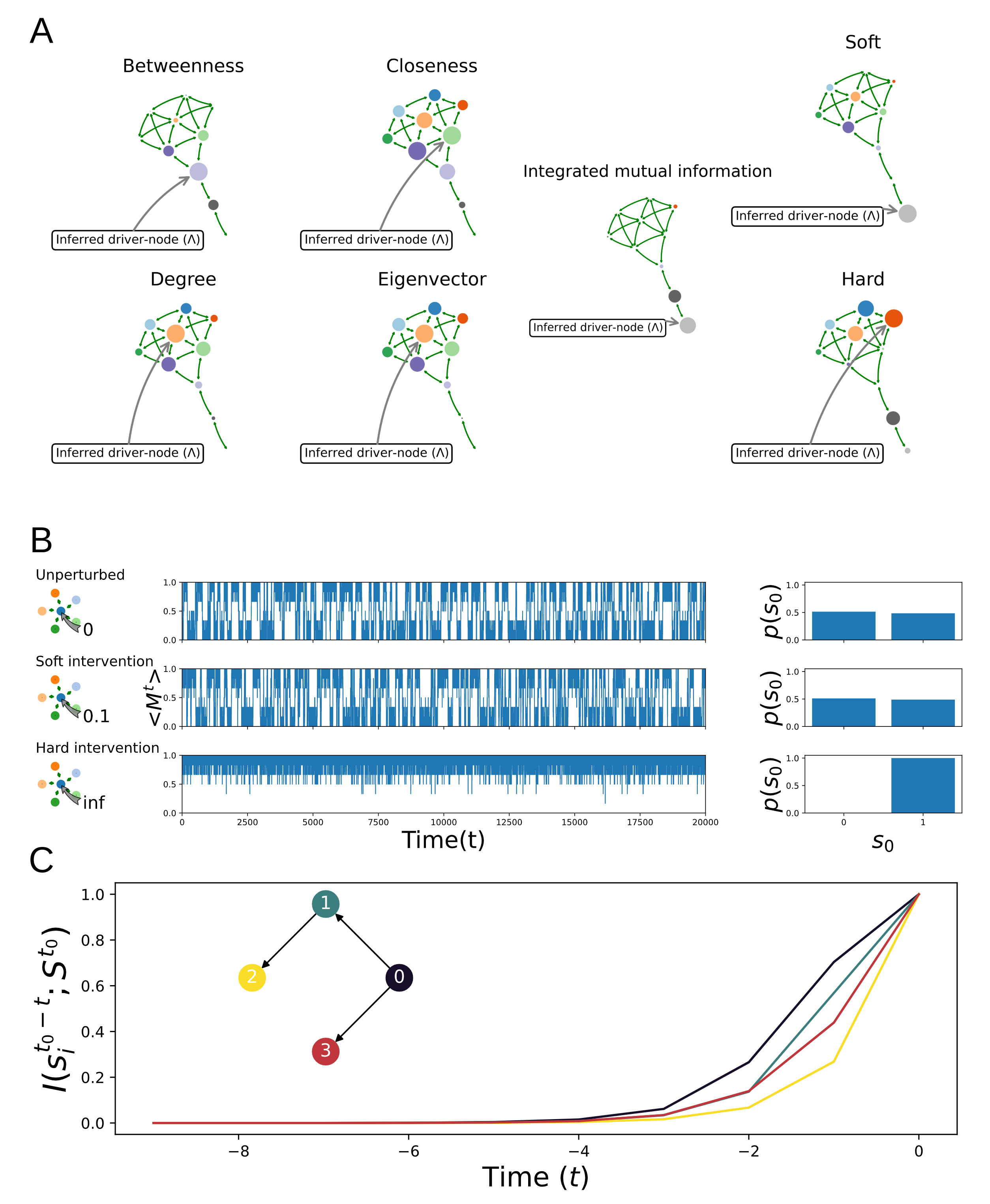
Figure 1: (A) Driver node inference. Dynamics are simulated using kinetic Ising spin dynamics. Causal interventions (soft and hard) are shown in the left column. Structural metrics (betweenness, closeness, degree, eigevenvector centrality) each produce different driver node estimates. Integrated mutual information predicts the driver node for soft causal interventions. High causal interventions produce different system dynamics (see B for an example) and different driver nodes. This figure show that dynamics interact with structure to produce non-trivial driver node estimates. In addition, causal intervention size (hard or soft) influence the observed system dynamics. (B) Effect of intervention size on system magnetization $<M^{t}>=\frac{1}{n}\sum_{i}s_{i}^{t}$ with kinetic Ising spin dynamics (see 2.1). Energy is added (gray arrow) to the nodal Hamiltonian of the blue node ($s_{0}$). (top) Non-Intervened system dynamics are shown with the distribution of the blue node $s_{0}$ (right). (middle) Soft intervention on node $s_{0}$ keeps similar dynamics as the non-intervened system dynamics. (bottom) Hard interventions yield profound different system dynamics compared to non-intervened dynamics. (C) Example of non-causal inflation of mutual information decay. The network structure is given by the graph inset; consisting of a system with 4 nodes in which each node is binary variable. Node 0 has a 50/50 distribution and all other nodes copy the state of its predecessor. Node 0 has the largest causal influence as it can influence the state of all other nodes in the system (over time). The information content of node 3 is biased; it stores the information from 0, but has no downstream causal effects. Yet, its information decay is similar to 1 which has one downstream node. The true driver node (0) has the largest information decay over time and is not confounded.

There will always be a minimal intervention size for which there is a measurable (i.e. non-zero) causal effect (eq. (7)), given finite amount of data. The causal impact will be maximal for hard interventions. As the intervention size is decreased so will causal impact. We hypothesize that there exists a lower bound for the soft interventions for which there will be a measurable causal impact. This minimal intervention size is dependent on the systems structure as well as the dynamics of the system and is difficult to determine a priori. Yet it is important to approach this minimum because if the intervention size is too large, then the intervened system dynamics will diverge from the non-intervened system dynamics, losing its representative capacity. Therefore, we estimate this minimum numerically, described further in section 3.2.

2.2.2 Intervention in kinetic Ising model

Nudge interventions are implemented by modifying the system Hamiltonian (eq. (5))

$$\mathcal{H}_{\textrm{nudge }s_{k}}(S)=-\sum_{i,j}J_{ij}s_{i}s_{j}-\sum_{i}h_{i}s_{i}-\eta s_{i}\delta_{ik}.$$ (8)

That is, an energy term is added to the intervened node $s_{k}$ by letting it interact with an external ‘spin state’ $\eta$. Both soft and hard interventions were used (see section 2.2.1). For hard interventions ($\eta\rightarrow\infty$) the nodal dynamics of the nudge node $s_{k}$ are no longer influenced by nearest neighbor interaction. That is, the node state for the intervened node $s_{j}$ will not change as a function of time. For soft interventions a grid-search was used with $\vec{\eta}:=\{\eta:\eta=0.55+i,i\in\{1,\dots,10\}\}$ to determine a minimal yet measurable intervention strength. Once determined the same $\eta$ was applied to each node in turn and this process is repeated for all networks in the experiments.

2.3 Measuring information flow

Each node in a dynamical system can be considered as an information storage unit [43, 42]. For example in social networks gossip can be considered as information one person possesses. Similarly, disease can be present in one city while being absent in another. Over time through interaction, this information stored in a node will percolate throughout the system while at the same time decaying due to noise. The longer the information of a node stays in the system, the longer it could affect the system dynamics. Therefore, dynamic impact of a node is upper-bounded by the amount of information a node shares with the entire system [41, 44, 42].

How does one measure information stored in a node? A node $s_{i}$ dictated by stochastic and ergodic dynamics can be considered a random variable. In Shannon information theory information is quantified in bits, i.e. yes/no questions concerning the outcome of a random variable. The average information that a random variable can encode is called entropy and is defined as:

$$\begin{split}H(s_{i})=-\sum_{s_{i}=x}p(x)\log p(x).\end{split}$$ (9)

Note all $\log$ are base 2 in this paper unless specified otherwise.

Entropy can also be interpreted as the amount of uncertainty of a random variable. In the extremes the random variable either conveys no uncertainty (i.e. a node always assumes the same state), or is randomly chosen between all possible states (uniform distribution). For example consider a coin flip. One may ask how much information does a single coin flip encode? If the coin is fair, i.e. there is equal probability of the outcome being heads or tails, the amount of questions needed to determine the outcome is exactly 1. In other words, a fair coin encodes 1 bit of information. However, when the coin is unfair the information encoded is less than one. In the extreme case where the coin always turns up heads, the entropy is exactly 0.

The information shared between a node state $s_{i}$ and a system state $S$ can be quantified by mutual information [41, 8, 44, 42, 26]. Mutual information can be informally thought of as a non-linear correlation function which inherits its properties from the Kullback-Leibler divergence. Formally, mutual information quantifies the reduction in uncertainty of random variable $X$ by knowing the outcome of random variable $Y$ [8]:

$$\begin{split}I(X:Y)&=\sum_{x\in X,y\in Y}p(x,y)\log\frac{p(x,y)}{p(x)p(y)}\\ &=H(X)-H(X|Y),\end{split}$$ (10)

where $p(x)$ and $p(y)$ are the marginals of $p(x,y)$ over $X$ and $Y$ respectively, and $H(X|Y)$ is the conditional entropy of $X$. The conditional entropy $H(X|Y)$ is similar to the entropy; it quantifies the reduction in uncertainty of the outcome $X$ by knowing the outcome of $Y$. Please note that the yes/no question interpretation even applies to continuous variables; although it may take an infinite amount of questions to determine the outcome of a continuous random variable.

2.3.1 Mutual information and causality

Consider an Markovian, isolated system consisting of two nodes $S=\{s_{i},s_{j}\}$ where $s_{j}$ causally depends on the previous state of $s_{i}$, encoded by a conditional probability distribution. We show here that the causal impact of $s_{i}$ on $s_{j}$ then reduces to mutual information.

For Markovian systems, the future state of the system is independent of its past given its present (eq. (2)). Therefore, we can write

$$\begin{split}p(s_{j}^{t+1}|S^{t})=p(s_{j}^{t+1}|s_{i}^{t}).\end{split}$$ (11)

For any two nodes $s_{i},s_{j}\in S$, the KL-divergence $D_{KL}(p(s_{j}^{t+1}|s_{i}^{t})||p(s_{j}^{t}))$ reduces to $I(s_{i}^{t+1};s_{j}^{t})$.

Theorem 1.

$E_{s_{i}}[D_{KL}(p(s_{j}^{t+1}|s_{i}^{t})||p(s_{j}^{t})]=I(s_{i}^{t+1};s_{j}^{t})$ when $s_{i}$ and $s_{j}$ have no common neighbors.

Proof:

$$\begin{split}E_{s_{i}^{t}}[D_{KL}(p(s_{j}^{t+1}|s_{i}^{t})||p(s_{j}^{t})]&=E_{s_{i}^{t}}\left[E_{s_{j}^{t+1}\mid s_{i}^{t}}\left[\log\frac{p(s_{j}^{t+1}\mid s_{i}^{t})}{p(s_{j}^{t+1})}\right]\right]\\ &=\sum_{s_{i}^{t}}p(s_{i}^{t})\sum_{s_{j}^{t+1}}p(s_{j}^{t+1}\mid s_{i}^{t})\log\frac{p(s_{j}^{t+1}\mid s_{i}^{t})}{p(s_{j}^{t+1})}\\ &=\sum_{s_{i}^{t}}p(s_{i}^{t})\sum_{s_{j}}\log p(s_{j}^{t+1}\mid s_{i}^{t})\log p(s_{j}^{t+1}\mid s_{i}^{t})-\sum_{s_{j}^{t+1}}p(s_{j}^{t+1})\log p(s_{j}^{t+1})\\ &=H(s_{j}^{t+1})-H(s_{j}^{t+1}\mid s_{i}^{t})\\ &=I(s_{j}^{t+1}:s_{i}^{t})\blacksquare.\end{split}$$ (12)

In this study, the entire system is considered as a downstream “node”. That is $I(S^{t+1};s_{i}^{t})$ is the causal information flow since does there cannot exist any confounding node, i.e. we consider systems where all variables are observed.

2.3.2 Integrated mutual information

In a network of nodes each causal relation (edge) is obviously not isolated, so confounding variables exist. Therefore, the mutual information between a node state and a future state $I(S^{t_{0}-t};s_{i}^{t_{0}})$ cannot be interpreted purely causal in general. Namely, this mutual information could in principle be created purely by another variable $s_{j}^{t_{0}-\omega}$ influencing both $s_{i}^{t_{0}}$ and $S^{t_{0}-t}$, even if there exists no causal influence from $s^{t_{0}}$ to any other variable.

Assuming the network itself is isolated, the only node for which the mutual information with a future system state could not have been fully created by a confounding variable is the driver node. That is, the driver node has the largest mutual information with the future system state. If this were fully induced by a confounding variable, then a different node would have to have even larger mutual information with the same future system state. In addition, this must hold for all future system states. By definition of the driver node, this cannot be true under the condition that the system isolated.

This point is illustrated in 1 C. Note that for all other nodes, however, it is possible for its mutual information value to be inflated due to non-causal correlations. This may result to a non-zero mutual information $I(s_{i}^{t_{0}-t}:s_{j}^{t})$ among the two variables even if they do not depend on each other in causal manner (fig. 1). Consequently, we define the integrated mutual information (IMI) for node $s_{i}$ as

where $S^{t_{0}}$ is the system state at some time $t_{0}$ and $s_{i}^{t_{0}-t}$ is the state of a node $t$ away from that system state. At time $t=0$ the value equals $I(s_{i}^{t_{0}};S^{t_{0}})=H(s_{i}^{t})$ for any node.

Here, undirected networks are considered. Due to detailed balance for undirected networks there exists a time symmetry in terms of variable dynamics. This means that for the systems considered in this study $I(s_{i}^{t_{0}-t};S^{t}_{0})=I(s_{i}^{t_{0}+t};S^{t}_{0})$ (see appendix 8.2). It is computationally easier to compute $I(s_{i}^{t_{0}+t};S^{t}_{0})$ rather than the reverse (see section. 3.2.2). For directed graphs, however, the meaning and interpretation of integrated mutual information changes depending on the direction in time it is computed (see appendix 8.2). This effect is outside the scope of the present study and will be the subject of future studies. For undirected graphs, the causal impact are time invariant and is equal forward and backward in time.

$$\begin{split}\mu(s_{i})=\sum^{\infty}_{t=t_{0}}I(s_{i}^{t_{0}-t};S^{t_{0}})\Delta t,\end{split}$$ (13)

For all ergodic Markovian systems the delayed mutual information $I(s_{i}^{t_{0}-t};S^{t_{0}})$ will always decay to zero as $t\rightarrow\infty$ [41, 8]. This decay is monotonic, which follows from the data-processing inequality [8] and states that information can never increase in Markov chains without external information injection (appendix 8.1). The question is how fast this decay takes place for each node (fig. 1 C), and consequently how much informational impact the node will have on the system.

Taking the entire system as a downstream ‘node’, $I(S^{t+1};s_{i}^{t})$ represents pure causal information flow for the driver node as long as there are no confounding variables. For the rest of the study we will therefore use the notation $I(s_{i}^{t_{0}+t};S^{t_{0}})$.

3 Methods and network data

3.1 Network data

3.1.1 Random networks

In total 16 Erdös-Rényi random networks were generated consisting of 10 nodes each. Each random network is generated by first drawing a random connection probability uniformly from [0,1], and then creating each possible undirected edge with probability $r$. Out of these 16 networks, ~82 percent had a single connected component (fig. 2). Each edge had unitary weight.

3.1.2 Real-world network: psychosymptoms

In addition to the generated random networks, we also test a small weighted network inferred from real data. This network differs from the random networks in that it is weighted and reflecting interactions among variables as a consequence of a real-world process, as well as reflecting inferred interactions from real data. The network data originates from the Changing Lives of Older Couples (CLOC) and compared depressive symptoms assessed via the 11-item Center for Epidemologic Studies Depression Scale (CES-D) among those who lost their partner (N=241) with still-married control group (N=274) [16]. Each of the CES-D items were binarized with the aid of a causal search algorithm using Ising model developed by [54] and represented as a node with weighted connections (fig. 5 D). For more info on the procedure see [54, 12, 16]. The 11 CES-D items are (abbreviated names used in the remainder of this text in brackets): ‘I felt depressed’ (depr), ‘I felt that everything I did was an effort’ (effort), ‘My sleep was restless’ (sleep), ‘I was happy’ (happy)‘, ‘I felt lonely’ (lonely), ‘People were unfriendly’ (unfr), ‘I enjoyed life’ (enjoy), ‘My appetite was poor’ (appet), ‘I felt sad’ (sad), ‘I felt that people disliked me’ (dislike), and ‘I could not get going’ (getgo).

3.2 Numerical methods

3.2.1 Magnetization matching

A prominent feature of the (kinetic) Ising model is the phase change that occurs as a function of noise (fig.2B)[19]. In this paper we tested whether the amount of noise would (i) affect which nodes becomes the driver node in the system, and (ii) whether the correct driver node could be predicted using either IMI or network centrality metrics. We tested three levels of noise (fig. 2 B); a low noise level (80% of the maximum magnetization), a medium noise level (70%), and a high noise level (60%) were used. This magnetization matching was achieved by estimating the magnetization curve as a function of $\beta^{-1}$ numerically.

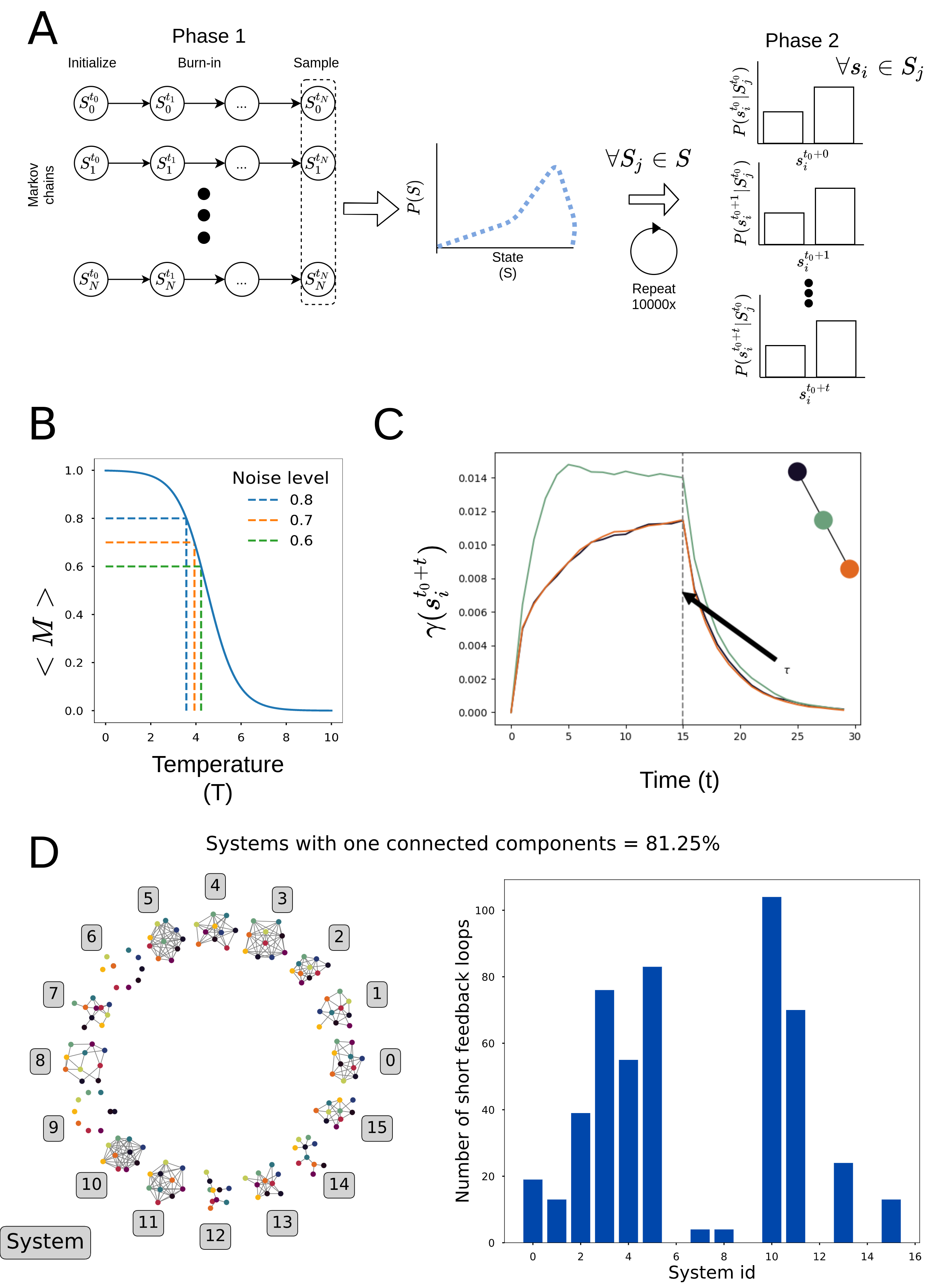
Figure 2: (A) Phase 1 initializes 10000 independent random Markov chains and equilibrated the chains for $t_{n}=1000$ time steps. The state distribution is estimated at $t_{n}=1000$ over the 10000 chains. In phase 2 for system states conditional distributions are estimated for $t$ time-steps from which mutual information is estimated $I(s_{i}^{t_{0}+t};S^{t_{0}})$. (B) Illustration of temperature matching. The graph depicts the conceptual transition between an ordered state (aligned spins) to a disorered state for the kinetic Ising on complex networks. The noise level was matched to the magnetization ratio of the max magnetization. For increase in temperature the noise level increases. (C) Illustration of applied interventions in an undirected 3 state system (top right corner). Each node is nudged according to eq. (7). The time prior to $\tau$ “pushes” the system dynamics out of equilibrium. From $\tau$ onwards the causal impact decays proportional to the causal impact a node has on the rest of the system. (D) Generated Erdös-Rényi networks. (left) Structure of each network, the number indicates the system id. (right)Number of triangles (feedback loops) for each system.

3.2.2 Estimating $p(S^{t_{0}})$ and $p(S^{t_{0}+t}|S^{t_{0}})$

For each noise level, $N=$1000$$ independent Markov chains are run for simulation with 1000 steps (fig. 2 A). Each chain was initialized with random state distribution over nodes. Each simulation step executes the following:

1. Pick a node at random from the system with equal probability;

2. Compute energy using eq. (5);

3. Flip the node state with probability eq. (4).

From this set, the equilibrium distribution over states $p(S^{t_{0}})$ was constructed in the form of sample of $N$ system states.

For this sample of system states, Monte-Carlo methods are similarly used to construct the conditional $p(s_{i}^{t_{0}+t}|S^{t_{0}})$. For each of the sample states $S_{i}\in S^{t_{0}}$, the procedure above was repeated 100000 times for 100 time steps in the psychosymptoms and 30 time steps for the random generated networks. All numerical experiments were repeated $n_{\textrm{trials}}=20$ times to provide confidence intervals for the results in all nudge conditions and temperature settings (noise conditions).

3.2.3 Time symmetry and mutual information

Thusfar, the definition of causal impact and IMI is ambiguous to the whether $t$ is positive or negative. Namely, if the node state $s_{i}^{t\pm 1}$ is captured in forward in time or backward in time with respect to some state $S^{t}$. For undirected networks with Ising spin dynamics there exists time symmetry with respect to how causal influence flows through the network due to detailed balance (see appendix 8.2). However, for directed networks this is not the case. The results obtained here are obtained using forward simulation in time only. The detailed balance condition ensures that the results would be symmetric when simulating the system backwards in time.

3.2.4 Area under the curve estimation

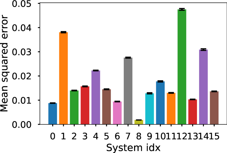
Figure 7: Average mean squared error $\pm 2SEM$ per system

The mutual information over time and KL-divergence over time were scaled for visual purposes in the range $[0,1]$ per trial set. A double exponential, $y=a\exp(-b(t-c))+d\exp(-e(t-f))$, was fitted to estimate these curves and subsequently IMI (eq. (13) and (7)) using least squares regression (fig. 3 C,5 C). The kernel showed to be a good fit as indicated by the low fit error (fig. 7, 8).

3.2.5 Sampling bias correction

Empirical estimates for mutual information are inherently contaminated due to sampling bias. In order to correct for this, Panzeri-Treves correction was applied [38]. This method offer a good performance in terms of signal-to-noise and computational complexity.

3.2.6 Driver node prediction and precision quantification

It is possible for two or more nodes to have exactly equal network structure features as well as node dynamics. For example consider a ring structure where each node has the exact same connectivity and all nodes have the same dynamics. In this case each node must have the same causal effect, and it would be impossible to disentangle these nodes causally from one another. Similarly graphs that are similar, e.g. show high degree of structural similarity but are not isomorphic, this causal separation may proof difficult for finite samples in stochastic settings as was discussed in 3.2.2. Consequently, we applied a parametric bootstrap procedure to estimate driver node sets (algorithm (10)).

Driver set estimation

The area under curve values, e.g. integrated mutual information and causal impact, were resampled to generate bootstrap distributions ( appendix 8.7). This creates a confidence interval for the integrated mutual information and causal impact. From these bootstrap distributions a driver node set is estimated (see algorithm (10) in appendix 8.7). The bootstrap procedure constructs driver node set $\Lambda$ iteratively by comparing the overlap $\phi$ with of the bootstrap for each variable with the distribution of the estimated driver node. For all experiments $\phi=0.5$. The driver node distribution was taken as the bootstrap distribution with the highest mean. Variables will be included to the driver node set $\Lambda$ if the overlap between its bootstrap distribution $i$ and driver node bootstrap distribution $j$ was $\phi_{ij}>0.5$. In total $N=1e4$ bootstrap trial were constructed of size $M=n_{\textrm{trials}}=20$; for each of the trials the average was computed. For each variables a Gaussian distribution was estimated over the $N$ bootstrap. This distribution was used for computing the overlap with the driver node distribution.

The bootstrap procedure cannot be applied to the network centrality metrics as there exists only one centrality rank assignment per network structure. Therefore, the driver nodes as inferred by maximum centrality metrics is the set of nodes ($\Lambda$) whose centrality metric ($f$) equals this maximum value, i.e.

$$\begin{split}\Lambda_{cent}=\textrm{argmax}f_{cent}(x):=\{x\in S:f_{cent}(s)\leq f(x)\forall s\in S\}\end{split}$$ (14)

where $f$ is the centrality function which assigns a real value to each node in the system. For degree centrality,

$$\begin{split}f_{deg}(a_{i})=\sum_{j}a_{ij}\end{split}$$ (15)

where $a_{ij}$ is the weighted connectivity between node $i$ and $j$ in the adjacency matrix $A$ of the network. If $a_{ij}>0$ node $i$ and $j$ are connected. In this study degree, betweenness, closeness or eigenvector centrality were used. (see section 8.6 for the formal definitions for the centrality measures).

Ground truth comparison

The ground truth values are the driver node estimations for the causal impact bootstrap distribution. Each estimator also generated a driver node set estimation. That is for integrated mutual information, degree centrality, closeseness centrality, betweeness centrality, eigenvector centrality, the bootstrap distribution generates an estimated driver set. To evaluate the performance of these estimators, an overlap score was computed with the ground-truth (causal impact estimation) using the Jaccard similarity metric:

$$J=\frac{A\cap B}{A\cup B}.$$ (16)

A Jaccard score of 1 means perfect overlap, i.e. the driver node set identified by causal impact and predictor set by IMI or one of the centrality metrics are identical. Conversely, a Jaccard score of 0 means completely disjoint driver-sets.

For every network, intervention size and temperature the similarity metric we computed the Jaccard score per predictor. Additionally, the relative performance ratio of the IMI predictor was evaluated by

$$\begin{split}R_{cent}=J_{IMI}-J_{cent}\end{split}$$ (17)

where $J_{cent}$ is the Jaccard score of the structural metrics (betweenness, closeseness, betweeness, eigenvector centrality). This performance indicator falls within [-1, 1] range: A value of -1 would indicate that the centrality metric correctly identified the driver node set; a score of 0 would indicate equal performance for the driver node identification between a centrality metric and IMI; a score of 1 would indicate a correct identification of the driver node for IMI, but a false identification of the centrality metric. The ratios were bootstrapped ($N=$100\,000$$) and tested for significance at $\alpha=0.01$. The driver node inferred performance is bound between $(0,\infty)$.

3.2.7 Software

A general toolbox was developed for analyzing any discrete systems using IMI, e.g. Susceptible-Infected-Recovered [34], Random Boolean networks [21]. The core engine is written in 3.07a with python 3.9.4 and offers C/C++ level performance, for more information see appendix 8.5.

4 Results

4.1 Random network results

Driver node inference accuracy is depicted in fig. 3 A for both IMI and the network centrality measures. Three crucial observations can be made from the Jaccard scores. First, for nearly all systems there exists an intervention size for which IMI obtains a Jaccard score of 1 (perfect true driver node inference), whereas this is not always the case for the centrality metrics, see e.g. system 3, 7, 15. Secondly, IMI is predictive nearly only for soft intervention sizes, i.e. intervention sizes smaller or of similar order of magnitude as the existing forces acting on nodes(i.e. their degree in the $J$ interaction matrix). In contrast, centrality metrics are mainly predictive for hard interventions. The statistical results reflect these observations (fig. 4 A and B).

In figure 3 B average decay curves are shown for IMI (top) and different intervention sizes (middle) and hard interventions (bottom) for the systems 2, 5, 12. Their network structure is depicted in fig. 3 B (top). Comparing hard interventions (bottom) with a more moderate intervention strength (middle) in system 2, shows that the driver node can significantly differ depending on the intervention size applied to the system. The order of the causal importance is noticeably different for the minimal intervention $\eta^{*}$ versus the strong intervention $\eta=\infty$ (middle and bottom plot in figure 3 B).

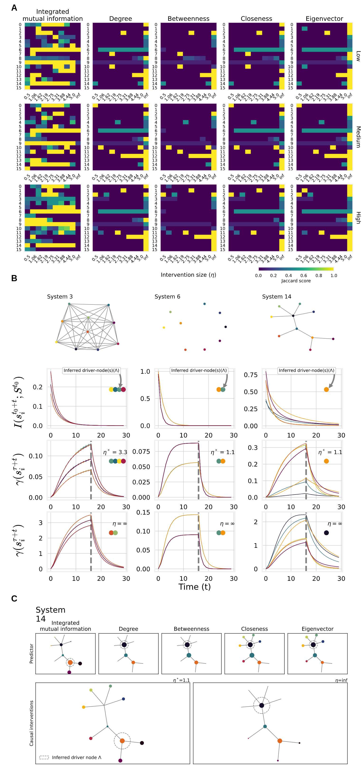
Figure 3: (A) Jaccard score per system (see figure 2 D for the various network structures) as a function of intervention size. Each row depicts an increase in noise indicated by the label on the right side of the plot. On average integrated mutual information is a better predictor for the driver node than the centrality metrics used in this study (see also fig. 4). Additionally, centrality metric tend to become predictor for hard interventions ($\eta=\infty$), whereas this is not the (generally) so for integrated mutual information. Hard interventions can cause different causal dynamics not present in unperturbed system dynamics (see B/C). Integrated mutual information is based on observations of the system. The Jaccord score indicates that integrated mutual information can infer driver nodes for unperturbed dynamics. (B) Example of typical experimental results. The figures highlight a selection from the generated random networks form A for the low noise condition. (top) The graph structure of the system and the mutual information decay curves (second from top). (second bottom and bottom) Show the causal impact decay for soft intervention $\eta^{*}$ and hard intervention $\eta=\infty$. The gray dotted line indicates $t=\tau$ where the nudge is removed from the system, the $t>\tau$ produces causal decay proportional to a node’s causal importance. For soft causal interventions the inferred driver node based on integrated mutual information (second from top) is predictive for the true causal driver node (second from bottom) with soft causal interventions. Importantly, the causal driver node may change as a function of the intervention size (second bottom vs bottom plot). The centrality metrics tend to not correctly identify the driver node (see C for an example). (C) Mutual information decay ($I(s_{i}^{t_{0}+t};S^{t_{0}+t})$) (top) and causal impact ($\gamma(s_{i}^{\tau+t})$ for minimal soft intervention $\eta^{*}$ (middle) and hard intervention (bottom).

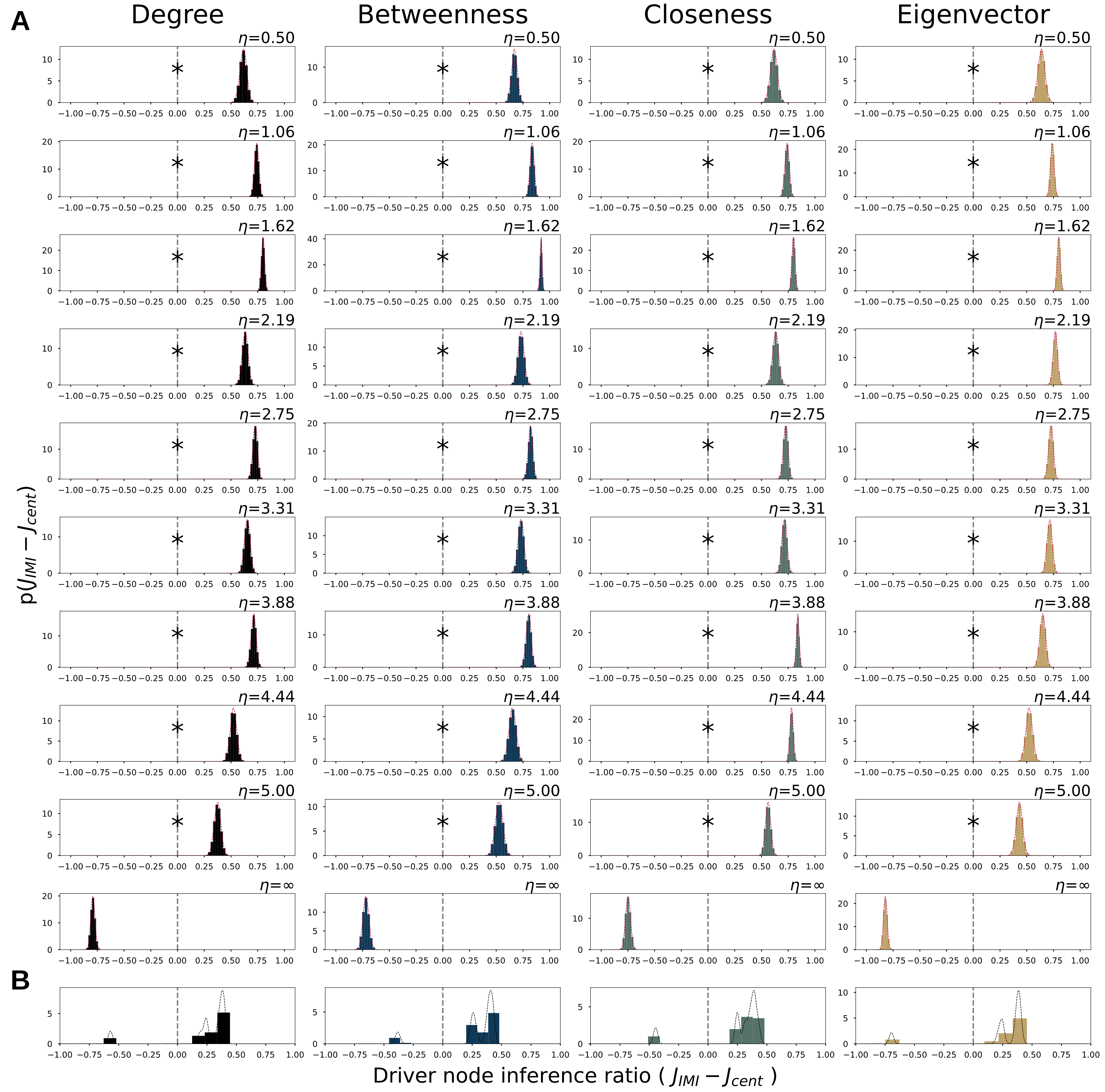
Figure 4: (A) Bootstrap results for driver node inference score $R_{cent}=J_{IMI}-J_{cent}$ per intervention size and for all interventions and noise levels(B). A kernel density is fitted for each distribution and integrated over the interval [-1, 0]. An inference ratio of 1 indicates that IMI is better a predicting the driver node than the structural metric and vice versa for a score of 0. Significant intervals are indicated by a asterisk * ($\alpha=0.01$). Except for the hard interventions ($\eta=\infty$) intervention size IMI is a better predictor than any of the network structural features.

4.2 Real-world network: psychosymptoms results

The psychosymptoms system reveals similar results to the random networks (fig. 5). Namely, for medium to high noise level IMI yielded significantly higher Jaccard scores than centrality metrics for low causal intervention (fig. 5 C/D, $p<<0.01$), while not for hard interventions. In contrast, hard interventions yield different causal structures altogether which do not reflect non-intervened dynamics (fig. 5 A/B). For example the true driver node under hard interventions identify ‘dislike’ (medium and high noise) to be the driver node (fig. 5 A ). Whereas for low causal intervention ‘sad’ is identified as driver node (fig. 5 A). This implies that intervention itself has impact on what causal structure is observed and that the intervention can show systemic behavior not present in the non-intervened system. The soft intervention of $\eta=0.1$ was too low to provide proper resolution for identification of driver nodes in the low noise setting (fig. 5 A). Hard intervention in low noise condition did provide a different driver node than the soft intervention. The grid-search for optimal $\eta^{*}$ was insufficient for the psychosymptom network and should be investigated in future studies.

In addition, the change in driver node observed in figure 5 A highlights one major flaw in centrality metrics: they cannot account for a change in driver nodes due to a change in dynamics. The implicit assumption on dynamics that each centrality metric holds, provides only one estimate per network structure. In contrast, IMI does not depend on what mechanisms generate system dynamics. Instead, it uses the distribution dictated by these system dynamics which match the true driver nodes.

Fried and colleagues postulated that ‘lonely’ was the gateway from which information spreads through the network, i.e. bereavement was embodied mainly by ‘loneliness’ which then percolated its effect to the other symptoms [16]. Since the data was cross-sectional, the comparison with the results from this study relies on the assumption that binary dynamics are representative of the absence and presence of psychological symptoms. If correct, the results from this study give a causal perspective on the associative results from [16]. The results from this study postulate that ‘depr’, ‘lonely’ and ‘sad’ have similar causal effect for moderate to high thermal noise.

It is important to emphasize that a quantification is given in terms of absolute effect size and not directed effects. This means that nudging for instance ‘sleep’ has some effect $X$ on the psycho-symptom network, in what direction that effect is, or whether it has a positive or negative effect on the bereavement score / cognitive load of the patient is not clear, and should be the subject of future studies (see appendix 8.4).

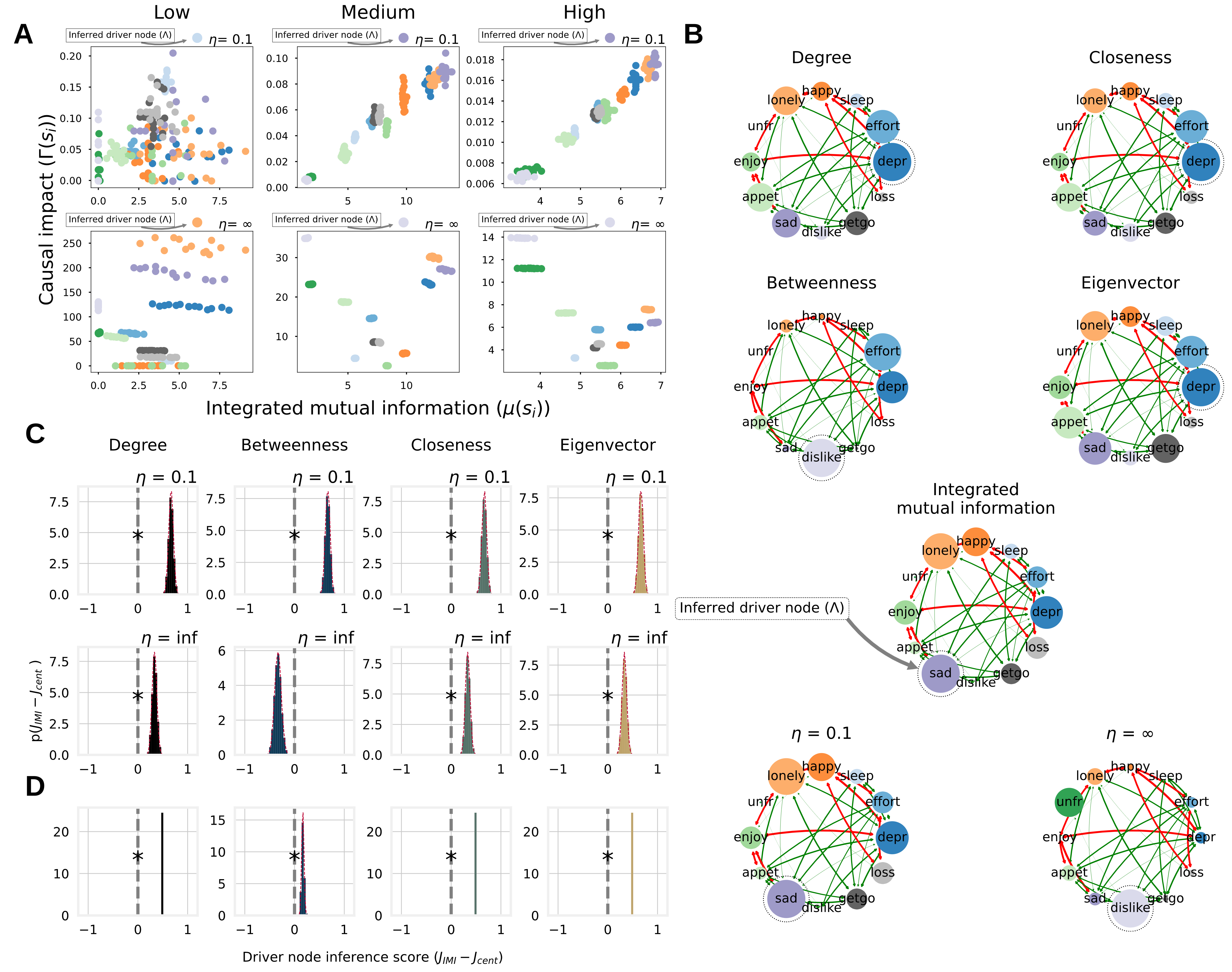
Figure 5: (A) Causal impact versus integrated mutual information for different noise levels and intervention sizes. The inferred driver node is indicated above each figure with a dot. For low noise level the numerical estimates were too noise and driver estimation was inaccurate. For intermediate to high noise level, causal impact scale linearly with integrated mutual information for soft interventions. Causal driver node was wrongly predicted for hard interventions by integrated mutual information. Notice how the causal flows change as a function of intervention size (top versus bottom plot). (B) Driver node identification in real-world network of psychosymptoms for medium noise as a function network features (top 4 subplots) and integrated mutual information (middle), and true causal driver nodes per intervention size (bottom). Integrated mutual information correctly identified the driver node with soft interventions, but not for high interventions. Only betweenness centrality correctly identified the true driver node for high causal interventions. (C) Bootstrap distributions for driver node inference score as function of intervention size across noise levels. A score of 1 indicates that integrated mutual information identified the driver node correctly, but the structural metric didn’t, and vice versa for a score of -1. In red kernel density estimates are indicated and integrated over [-1, 0]. The asterisk (*) indicates a significant better inference score for integrated mutual information ($\alpha<.01$). Integrated mutual information was a better predictor than any of the network features for soft interventions. (D) Bootstrap distribution for driver node inference score as function of temperature and nudge size. The integrated mutual information was a significant better predictor across noise and intervention size ($\alpha<0.05$ indicated by *).

5 Discussion

Structural metrics can be considered as implicitly assuming a particular dynamics [5, 4]. For example, the eigenvector centrality has a clear analytical connection with linear dynamics, such as a simple diffusion process. Betweenness centrality on the other hand can be considered to assume that causation between nodes is transmitted mainly along the shortest paths between pairs of nodes (see appendix 8.6), such as in message or package routing. Finally, many more network centrality metrics have been developed based on specific dynamics, such as current and flow centrality measures. Thus, such network structural metrics could indeed be used, but a careful analysis of the dynamic equations is required to assess which centrality measure (if any) turns out appropriate.

The results from this study show that high degree nodes with Ising spin dynamics tend to actually not be a driver node for small interventions. In this model it can be understood since high degree nodes exhibit “frozen” behavior; their large(r) number of neighbors effectively sum up to a constant and strong force towards the majority state. Consequently, a constant (soft) intervention will be relatively ineffective with hubs. For non-intervened Ising dynamics, it makes intuitive sense that the dynamics are driven by the nodes which are neither “frozen” (hubs) nor are poorly connected (low-degree nodes), which is reflected by the soft intervention setting. This insight is specific to the Ising system but illustrates that the information flow and causal flow of a system is not merely determined by the connectedness of a node in the network. Rather, the connectedness of the entire system in addition to inter-node dynamics combined are crucially important for causal flows and driver node identification.

The results further imply that for unperturbed dynamics structural metrics may not be predictive for determining the causal importance of nodes. Soft interventions revealed different causal structure than hard interventions (fig. 3 5). For hard interventions, structural metrics do become predictive for causal importance for the networks studied here. However, the dynamics of these systems are shown to deviate from the non-intervened dynamics, causing system dynamics that are not representative of the non-intervened system. This can be seen in the causal influence in figure 3 and 5 where the causal influence for hard interventions is opposite to soft causal interventions. Consequently, if the aim is to provide understanding to the information flows for non-intervened dynamics, then hard interventions are not preferred.

In addition, the results imply that in order to achieve maximum impact for a fixed ‘intervention’ budget (injected energy), choosing the high degree nodes is not necessarily optimal. The adjusted Hamiltonian (eq. (8)) introduces a bias on low degree nodes. Here, a causal intervention was performed by adding fixed energy to the Hamiltonian. For fixed intervention size $\eta=c$, the causal impact on the nodal distribution will be relatively higher for nodes with low degree than nodes with higher degree. Higher degree nodes may have higher causal effect in principle if the same probability mass is changed. However, moving the same probability mass scales non-linearly in kinetic Ising (eq. (5)). For a limited ‘intervention budget’ it is preferred to locate those elements of the system that reaches maximal causal effect.

For, some systems, however, the inferred driver node never matched the true driver node(s) (e.g. system 8 in fig. 3). This could be due to two main reasons. First a grid-search was applied for the intervention size. It was argued that there would be a minimal intervention $\eta^{*}$ which would lead to a measurable effect. It is possible that the parameter space used here missed the intervention size that provided enough resolution to accurately determined the driver node(s). Second, the numerical procedure for driver node inference could be optimized. The overlap of distribution was set to $\phi=0.5$, to infer the driver node set $\Lambda$, to prevent false positives for driver node identification due to noise in observed system states. However, the choice of parameter was not optimized and could lead to ambiguous driver node inference. System 8 in particular was most nodes in the network had a similar connectivity pattern, and as such causal isomorphy occurs, i.e. the causal importance of a node is indistinguishable from any other node in the system. The bootstrap estimates led to high level but not perfect of overlap (see appendix 8.7). Consequently, if $\phi$ was set differently, the inferred driver nodes could be improved. In future studies, we aim to further look into what how this numerical procedure could be improved for inferring driver nodes in dynamical networks particularly for causal isomorphic nodes.

5.1 Limitations

The systems considered are discrete and ergodic. IMI assumes that the data-processing inequality holds for the system(section 2.3.2). The data-processing inequality in ergodic systems ensures that $I(s_{i}^{t_{0}+t};S^{t_{0}})$ monotonically approaches zeros as $t\rightarrow\infty$ (see appendix 8.1). As a consequence IMI will always be finite for ergodic systems. For non-ergodic systems, the data-processing inequality can only guarantee that $I(s_{i}^{t_{0}+t};S^{t_{0}})$ never increases as a function of $t$. Namely, the data-processing inequality ensures that no local manipulation of information may increase the information content of a signal. This implies that as $t\rightarrow\infty$, IMI may not converge for nodes with non-zero baselines. For these cases, however, it is possible determine the driver nodes by considering finite time-scales, or subtracting the asymptotic $\gamma$ value and reporting it separately.

In addition, we merely studied on type of dynamic here, i.e. the kinetic Ising model. Integrated mutual information does not assume a particular type of dynamic, i.e. it merely requires the data processing inequality to be true. We believe that the methods proposed here can readily be applied to other ergodic systems with different kinds of dynamics and produce reliable estimates for the driver node under theoretical constrains used in this study (see 2). However, future work would need to study these claims in more detail.

Systems of size at most $n=12$ were used. The size of the system was chosen due in order to provide high reliability of the probability distributions. In addition, larger graphs can be decomposed in various different network motifs [1]. It is believed that these motifs form the “computational” buildings blocks for larger complex systems under the assumption of nearest neighbor interactions. That is, understanding the motifs would gain insights in how a macroscopic property emerges from local interactions. The aim of this study was to relate structural connectedness to dynamic importance; the exact nature or occurence of motifs were not the focal point. In real-world systems, however, it is exactly the composition and interaction of these motifs that are vital to complex systems. Here, the motifs were implicit on the real-world network and the generated structures. We leave it up to future work to map out the driver nodes of common network motifs in different dynamics using and relate the structural importance to the dynamical importance.

6 Conclusions

Our results indicate that dynamic importance cannot necessarily be reliably inferred from network structural features alone, demonstrated here using kinetic Ising spin dynamics. The goal of this paper was to show that structural methods can provide unreliable estimates of the driver node in dynamical systems. The results from this study show that the common assumption of structurally central or well-connected nodes being simultaneously dynamically most important is not necessarily true. This implies that we cannot abstract away the dynamics of a dynamic system before inferring driver nodes. The proposed information theoretic metric, integrated mutual information (IMI), was better able identify the driver node for non-intervened dynamics in systems. Importantly, IMI does not require knowing the dynamics equations and/or the network structure of the system. It is instead calculated directly from a cross-section of time-series of the system without interventions. The proposed metric could potentially be useful in applications with rich data sets and where performing interventions are infeasible or impractical.

7 Acknowledgment

This research is supported by grant Hyperion 2454972 of the Dutch National Police. In addition, Rick Quax acknowledges funding from the European Union’s Horizon 2020 research and innovation program under grant agreement No 848146 (ToAition).

We thank M.Sc. Fiona Lippert, Dr. Paul Duijn and Dr. Thijs Vis for fruitful discussions in support of this paper. We declare that no conflict of interests are present in the conduction of this study.

8 Appendix

8.1 Data-processing inequality

The data-processing inequality can be used to show that no clever manipulation of the data can improve the inferences made from that data (see for more detail [8]).

Definition 1.

Random variables $X\rightarrow Y\rightarrow Z$ are said to form a Markov chain if the conditional distribution of $Z$ depends only on $Y$ and is conditionally independent of $X$. Specifically, $X,Y,Z$ form a Markov chain if the joint probability can be written as:

$$\begin{split}p(x,y,z)=p(x)p(y|x)p(z|y)\end{split}$$ (18)

Theorem 2.

(Data-processing inequality) If $X\rightarrow Y\rightarrow Z$, then $I(X;Y)\geq I(X;Z)$.

Proof: By the chain rule, the mutual information can be expanded in two different ways:

$$\begin{split}I(X;Y;Z)&=I(X;Z)+I(X;Y|Z)\\ &=I(X;Y)+I(X;Z|Y)\end{split}$$ (19)

Since $X$ and $Z$ are conditionally independent given $Y$, we have $I(X;Z|Y)=0$. Conversely, if $I(X;Y|Z)\geq 0$, this would give

$$\begin{split}I(X;Y)\geq I(X;Z).\end{split}$$ (20)

Thus we only have equality if and only if $I(X;Y|Z)=0$ for Markov chains. Similarly, one can prove that $I(Y;Z)\geq I(X;Z)\blacksquare$.

Corollary 1.

If $Z=g(Y)\rightarrow I(X;Y)\geq I(X;g(Y))$

Proof: $X\rightarrow Y\rightarrow g(Y)$ forms a Markov chain $\blacksquare$.

This result implies that no function $g(Y)$ can increase the information about $X$.

Corollary 2.

If $X\rightarrow Y\rightarrow Z$, then $I(X;Y|Z)\leq I(X;Y)$

From eq. (19) it is noted that $I(X;Z|Y)=0$ due to the definition the Markov chain and $I(X;Z)\geq 0$. Therefore:

$$\begin{split}I(X;Y|Z)\leq I(X;Y)\blacksquare\end{split}$$ (21)

The dependence of $X$ and $Y$ is decreased or remains unchanged by the observation of a “downstream” random variable $Z$. For any complex system in which the state distribution follows a Markov chain, i.e. $X^{t_{0}}\to X^{t_{0}+1}\to\dots\to X^{t_{0}+\infty}$. The mutual information $I(X^{t_{0}};X^{t_{0}+t})$ will always decay to zero as $t\to\infty$.

8.2 Mutual information and time symmetry

The methods applied in the main text imply that the metric can be used symetrically. In this study time-delayed mutual information was performed in a ‘forward’ manner for pratical purposes. Namely, the system state was simulated for positive $t$ from some $t_{0}$. For undirected networks there is a symmetry with regard to where information flows. Information is not bounded by any directionality of edges (fig. 6(b)).

It is important to emphasize that this (generally) is not the case for directed networks. If information is constricted to flow in one direction, the mutual direction of time simulation is crucial. Additionally, directed networks show that the metric can be applied for different purposed. This can be seen in fig. 6(a), where forward simulations gives ‘information sinks’ and backward simulation provides ‘information sources’. IMI in directed networks will provide information about what nodes receive the most information over time. In contrast, simulating backwards shows what nodes have most impact on the instantaneous state of the system. This dual-use of information will be the focus of future studies.

8.2.1 Time reversibility and detailed balance

In order to show that $I(s_{i}^{t+1};S^{t})=I(s_{i}^{t-1};S^{t})$, we have to show that $p(S^{t+1}_{*}|S^{t}_{*})=p(S^{t-1}_{*}|S^{t})$.

Two-sided Markov Chains

For a positive recurring Markov chain $\{S^{t}:t\in\mathbb{N}\}$ with transition matrix $P$ and stationary distribution $\pi$, let $\{S^{t}_{*}:t\in\mathbb{N}\}$ a stationary version of this chain, i.e. $S^{0}\sim\pi$. We can construct a two-sided extension of $S^{t}$ by defining a shift $k\geq 1$, extending the process $S$ backwards in time: $S^{t}_{*}(k)=S^{t-k}_{*}$ with $0\leq k<\infty$. It is true that by stationarity $S^{t-k}_{*}$ has the same stationary distribution as $S^{t}$: we arrive at $\{S^{t}_{*}:t\in\mathbb{Z}\}$.

Detailed balance

Let $\{S^{t}_{*}:t\in\mathbb{Z}\}$ be a two-sided extension of a positive recurrent Markov chain with transition matrix $P$ and stationary distribution $\pi$. A transition from state $i$ to $j$ is denoted with notation $i\rightarrow j$.

$$\begin{split}p(S^{1}_{*}=j|S^{0}=i)&=p(S^{1}_{*}(k=1)=j|p(S^{0}_{*}(k=1))=i)\\ &=p(S^{0}_{*}=j|S^{-1}_{*}=i)\\ &=\frac{p(S^{-1}_{*}=i|S^{0}_{*}=j)p(S^{0}_{*}=j)}{p(S^{-1}_{*}=i)}\\ &=\frac{\pi_{j}}{\pi_{i}}P_{i\rightarrow j}\end{split}$$ (22)

In other words the time-reverse Markov chain is a Markov chain with transition probabilities:

$$\begin{split}P_{i\rightarrow j}\pi_{i}=\pi_{j}P_{j\rightarrow i}\end{split}$$ (23)

This is also known as detailed balance. In the manuscript, ergodic systems are used and therefore satisfy the time-symmetry. This results that $I(s_{i}^{t+1};S^{t})=I(s_{i}^{t-1};S^{t})$.

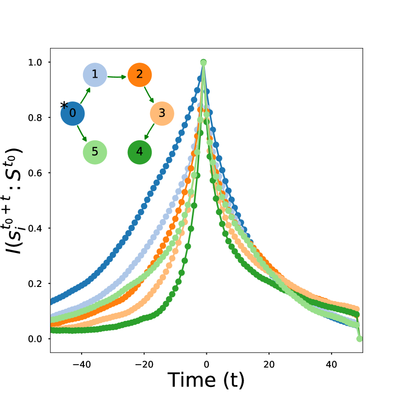
(a)

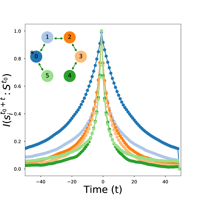
(b)

Figure 6: Example of time symmetry in directed and undirected networks. Figure 6(a) shows the asymmetry that occurs when information flow is directed. The time before the system state $t<t_{0}$ can be interpreted as information sending. Namely, nodes that have the most impact on the current system state $S^{t_{0}}$. In contrast, information for $t>t_{0}$ as information receiving; nodes that receive information from $S^{t_{0}}$. The most striking example is node 4 which has a sharp decay for $t<t_{0}$ but a relatively fat tail for $t>t_{0}$. This change is due to the difference in meaning of the IMI, e.g. sending vs receiving.
figure 6(b) shows that for undirected networks there is no difference between node importance before or after $t_{0}$; information flows both directions.

8.3 Data correction and fit errors

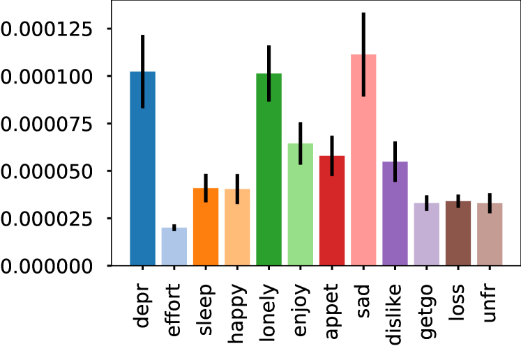
Figure 8: Average mean squared error $\pm 2SEM$ for psychosymptom system.

8.4 Validation of psychosymptoms

The results from this study imply that for low thermal noise not enough resolution was possible to reliably estimate the driver node. For medium to high noise levels, the ‘sad’ emerged as the driver node.

In the original study, the bereavement score was most affected by ‘lonely’, and showed weak negative associations with ‘happy’ and ‘effort’ (fig. 9 adopted from [16]). Consequently, it seems that medium to high thermal noise is most congruent with the original study. Fried and colleagues postulated that ‘lonely’ was the gateway from which information spreads through the network, i.e. bereavement was embodied mainly by ‘loneliness’ which then percolated its effect to the other symptoms. Since the nature of the data was cross-sectional, the comparison with the results from this study relies on the assumption that binary dynamics are representative of the absence and presence of psychological symptoms. If correct, the results from this study give a causal perspective on the associative results from [16]. The results from this study postulate that ‘depr’, ‘lonely’ and ‘sad’ have similar causal effect for moderate to high thermal noise.

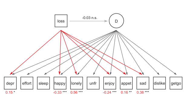
Figure 9: Main results from Friend and colleagues [16]. The network represents the output from a Multiple Indicators Multiple Causes (MIMIC) model. The red lines indicate significant direct effects of spousal loss on Center for Epidemological Studies Depression Scale(CES-D items); standardized estimates of these affects are represented in red below the symptoms. There was no significant loading of loss on the latent factor $D$. For more info see [16].

It is important to emphasize that a quantification is given in terms of absolute effect size and not directed effects. This means that nudging for instance ‘sleep’ has some effect $X$ on the psycho-symptom network, in what direction that effect is, or whether it has a positive or negative effect on the bereavement score / cognitive load of the patient is not clear, and should be the subject of future studies.

As a final note, the field of psychometrics is concerned with relating how observables (e.g. behavior, responses on questionnaires, etc) relate to theoretical cognitive constructs such as intelligence or mental disorders. A common approach in understanding high level phenomena such as depression is to use a latent variable model, i.e. assuming some high abstract feature to be the cause of the observables (or vice versa). Only recently has this paradigm shifted from a latent variable model to a network based approach [55, 11, 6]. Marsman et al. recently reconciled these two approached by showing statistical equivalence between the Ising model and canonically used latent variable models in psychometrics [36]. The two approaches thus highlight different aspects in theory building; measurement invariance and correlation structure may be interesting from a common cause approach but not from a network perspective which is more interested in dynamical aspects of the system. Both approaches, however, aid in highlighting different aspects of the psychological constructs.

8.5 Code manual

Accompanying this paper, I developed a general framework for analyzing discrete systems using IMI. The code is written in python 3.7.2 and uses cython 0.28.2 for c/c++ level performance. The code is freely available on cvanelteren.github.io includes the latest build instructions.hat follows here is a brief overview of the framework.

8.6 Structural methods

Network analysis has traditionally resulted in analyzing the structure of the network. A fundamental concept within network science is centrality, and how to measure the centrality of nodes has become an essential part of understanding networked systems such as social networks, the internet, biological networks, traffic and ecological networks. At its core, a centrality measure quantifies the ‘importance’ of a node based on some structural property. It allows ranking nodes based on a real-valued function.

There is, however, a long-standing debate concerning what centrality metrics actually measure for networked systems [7, 4, 5, 49] . From a network theoretical perspective most centrality measures, e.g. betweenness, closeness, eigenvector and degree centrality, essentially classify the ‘walk structure’ of a network [4, 5]. A walk from node $i$ to node $j$ is a sequence of adjacent nodes that begins with $i$ and ends with $j$. The structure of walks can be divided along different criteria. For example a trail is a walk in which no edge (i.e. adjacent pair of nodes) is repeated. In contrast, a path is a trail in which no node is visited more than once. Similarly, one could define a walk structure by only using the shortest path from one node to another, or by using random movements between nodes (random walks).

Alternatively, from a complex systems perspective, centrality metrics implicitly assume dynamics on the network structure. Betweenness centrality for example, computes centrality based on how often a node acts as a bridge along the shortest path between two other nodes. If one assumes that the network has dynamics $D$ where information between nodes follows the shortest path, this metric may be a valid description to use and identify dynamically important nodes.

In the best case, a centrality metric is fully predictive for identifying important nodes a complex system. Consequently, the centrality metric can be used to understand the system. However, an issue with the use of centrality metrics is determining which centrality metric to use. Consider for example figure 1 A; different centrality metrics can identify different nodes as most central. This has lead to the common observation that some centrality measures can ‘get it wrong’ when the aim is to predict dynamical important structure in networked systems. Additionally, the ranking produced through some centrality metric does not quantify inter-rank differences. This potentially leads to underestimation of nodal influence when used in dynamic context [49].

We will show how centrality measures have no meaningful prediction power of the most causal node in nodes dictated by the Gibbs measure. We are aware that centrality measures do not embody the full extent of what structural methods embody, or what network science in particular has to offer. However, many structural methods share the common characteristics listed above, i.e. they quantify the walk structure of a network. For our analysis, we used the weighted variants of degree centrality, betweenness centrality, information centrality, and eigenvector centrality. What follows is a brief description of commonly used centrality metrics.

8.6.1 Degree centrality

Degree centrality is the best-known measure of all the centrality measures. It is often thought that degree centrality is indicative for the dynamic importance of a node. This intuition is based on the concept of flow: the more connection a node has, the more interaction potential that node has and therefore the more important a node must be. Freeman defined centrality measure as the count of the number of edges incident upon a given node [15]:

$$c_{i}^{\textnormal{deg}}=\sum_{j}a_{ij}$$ (24)

where $a_{ij}$ is the row/column of node $i$ in the adjacency matrix $A$ of the network. Please note that the entries $a_{ij}$ are weighted and not binary.

8.6.2 Betweenness centrality

Betweenness centrality quantifies the number of times a node acts as a bridge along the shortest path between two other nodes. It was introduced as a measure for quantifying the control of communication among humans in social networks by Freeman [15]. Nodes that have a high probability to occur on a randomly chosen shortest path between two randomly chosen vertices have a high betweenness. Formally, this can be written as:

$$\begin{split}c^{\textrm{betw}}_{i}=\sum_{j,k}\frac{\sigma(j,k|i)}{\sigma(j,k)}\end{split}$$ (25)

where $\sigma(j,k)$ represents the number of shortest paths between node $j$ and $k$, and $\sigma(j,k|i)$ is the subset that goes through node $i$. We use the normalized version of betweenness that divides the betweenness score by the number of pairs of vertices (not including node $i$);

$$\begin{split}c^{\textrm{betw}}_{i}&=\frac{1}{Z}\sum_{j,k}\frac{\sigma(j,k|i)}{\sigma(j,k)}\\ \ Z&=\frac{((n-1)(n-2))}{2}\end{split}$$ (26)

8.6.3 Closeness centrality

Closeness centrality is defined as the reciprocal sum of the length of the shortest paths between the node $i$ and all other nodes in the network $j\in N$:

$$c^{\textrm{close}}_{i}=\frac{1}{\sum_{j}^{N}d(i,j)}.$$ (27)

From a complex system perspective it assumes that information is transferred along its shortest paths. A node with short distance to many other nodes will be able to quickly transfer its information to other nodes in the network.

8.6.4 Eigenvector centrality

Eigenvector centrality is the most difficult centrality measure to give an intuitive feeling for. Where $A$ is the adjacency matrix of the system, eigenvector centrality of node $i$ is defined as:

$$\begin{split}c^{\textrm{ev}}_{i}=\frac{1}{\lambda}\sum_{j}a_{ij}x_{j}\leftrightarrow Ax=\lambda x\end{split}$$ (28)

For any square matrix of rank $n$, the matrix will have at most $n$ eigenvector-eigenvalues pairs. A common choice for eigenvector centrality is motivated by The Perron-Frobenius theorem, and involves choosing the eigenvector $x$ with the largest eigenvalue $\lambda$ [10, 17]. This has the desired property that if $A$ is irreducible, or equivalently if the network is strongly connected, that the eigenvector $x$ is both unique and positive.

The sign and size of the eigenvalue are important for the relation between the value and importance of a node. In linear differential equations negative eigenvalues correspond to non-oscillatory exponentially stable solutions. In contrast, in difference equations it indicates an oscillatory behavior. Geometrically speaking, negative eigenvector embodies a linear transformation across some axis.

Intuitively speaking, eigenvector centrality quantifies the influence of a node in the network. It assigns relatives scores to all nodes in the network based on the concept that connections to high-scoring nodes contribute more to the score of the node in question than equal connections to low-scoring nodes. A high eigenvector score implies that the node is connected to many other nodes that themselves have high scores. Google PageRank and Katz centrality are variants of eigenvector centrality [30]. A node with high eigenvector centrality is not necessarily a node that has many connection (incoming or outgoing). For example a node may have a high eigenvector centrality if it has few connections, but those connections are connected to nodes that are of high importance.

8.7 Bootstrap distributions

A total of $10\,000$ bootstrap samples were conducted with replacement. For each nodal bootstrap distribution a gaussian kernel density was estimated. The node with the highest causal impact was chosen as the initial driver set $\Lambda$. Then the overlap $\phi$ between this driver node and the remaining nodes in the system was computed iteratively. We considered the overlap $\phi=0.5$ or higher was sufficient for the node was to be considered causally similar to the driver node. Therefore, the proposed node will be included in the driver node set if $\phi\geq 0.5$.

8.7.1 Numerical procedure

⬇

def bootstrapDrivers(D, N, M, phi=0.5) -> dict:

"""

Determines driver-nodes through the boostrap distribution It consists as an

iterative procedure that takes the max value in the data, then a normal

distribution is fitted an tested with overlap for the other nodes in the

data at ‘phi‘

\parParameters

———-

D: np.array

2d matrix consisting of size n_features x n_observations

N: int

Total number of samples used for bootstrap

M: int,

number of draws for each of each bootstrap sample

phi : float

Overlap between distribution.

\parReturns

———-

dict of driver-nodes under overlap ‘phi‘

"""

# part of standard library python

from statistics import NormalDist

import numpy as np

\par# generate subsamples

n_features, n_obs = D.shape

D_bar = np.zeros((n_features, N))

# sample from observations

for var in range(n_features):

D_bar[var] = np.random.choice(D[var], size=(N, M)).mean(1)

\par# create bootstrap distribution

driver = D_bar.mean(1).argmax()

driverDist = NormalDist().from_samples(D_bar[driver])

\par# other nodes to consider

drivers = {} # Lambda

options = np.arange(n_features)

for var in options:

# fit distribution

otherDist = NormalDist().from_samples(D_bar[var])

# compute overlap

overlap = driverDist.overlap(otherDist)

if overlap > phi:

drivers[var] = (otherDist.mean, otherDist.variance)

return drivers

Figure 10: Driver node detection algorithm in python.

8.7.2 Erdös-Rényi networks

Bootstrap distribution kernel density estimates for Erdös-Rényi networks. X indicates area under the curve for mutual information or causal impact respectively. Note $x$ here refers to the input variable which are the area under curves either for integrated mutual information ($\eta=0$) or for causal impact $\eta>0$.

8.7.3 Psycho networks

Note $x$ here refers to the input variable which are the area under curves either for integrated mutual information ($\eta=0$) or for causal impact $\eta>0$.

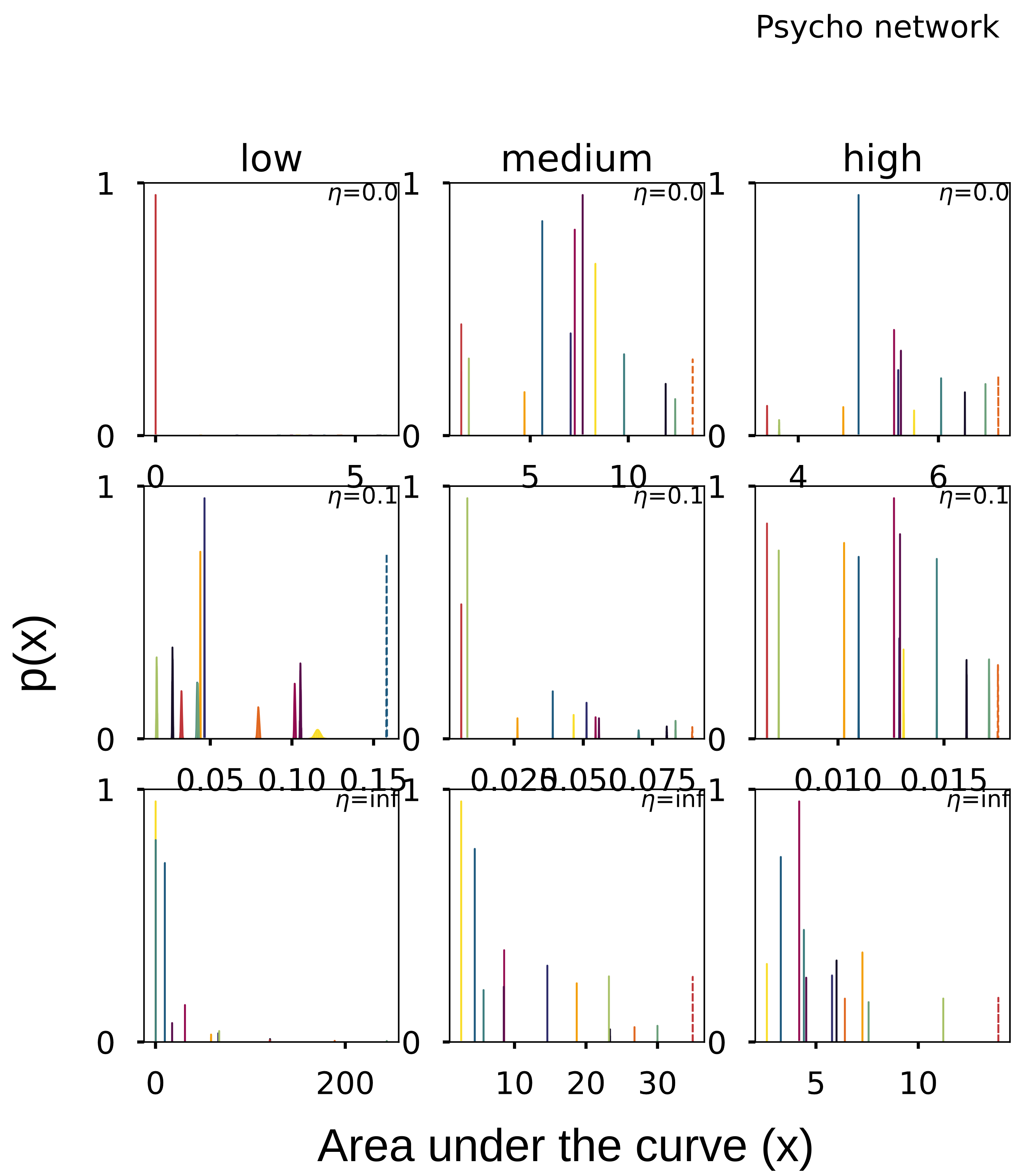
Figure 11: Bootstrap distribution for psychosymptom network. Driver node is indicated by a dotted line.

References

- [1] Uri Alon “Network Motifs: Theory and Experimental Approaches” In Nature Reviews Genetics 8.6, 2007, pp. 450–461 DOI: 10.1038/nrg2102
- [2] Nihat Ay and Daniel Polani “Information Flows in Causal Networks” In Advances in Complex Systems 11.01, 2008, pp. 17–41 DOI: 10.1142/S0219525908001465
- [3] Baruch Barzel and Albert-László Barabási “Universality in Network Dynamics” In Nature Physics 9.10 Nature Publishing Group, 2013, pp. 673–681 DOI: 10.1038/nphys2741
- [4] Stephen P. Borgatti “Centrality and Network Flow” In Social Networks 27.1, 2005, pp. 55–71 DOI: 10.1016/j.socnet.2004.11.008
- [5] Stephen P. Borgatti and Martin G. Everett “A Graph-Theoretic Perspective on Centrality” In Social Networks 28.4, 2006, pp. 466–484 DOI: 10.1016/j.socnet.2005.11.005
- [6] Denny Borsboom et al. “The Small World of Psychopathology” In PLoS ONE 6.11, 2011 DOI: 10.1371/journal.pone.0027407
- [7] Laura F Bringmann et al. “What Do Centrality Measures Measure in Psychological Networks ?”, 2018, pp. 1–34 DOI: 10.13140/RG.2.2.25024.58884
- [8] Thomas M. Cover and Joy A. Thomas “Elements of Information Theory” In Elements of Information Theory, 2005 DOI: 10.1002/047174882X
- [9] Fabian Dablander and Max Hinne “Node Centrality Measures Are a Poor Substitute for Causal Inference” In Scientific Reports 9.1 Springer US, 2019, pp. 1–13 DOI: 10.1038/s41598-019-43033-9
- [10] P. Debye and P. Scherrer “Werk Übergeordnetes Werk” In Nachr. Ges. Wiss. Göttingen, Math.-physik. Klasse 2, 1918, pp. 101–120
- [11] Sacha Epskamp, Denny Borsboom and Eiko I. Fried “Estimating Psychological Networks and Their Accuracy: A Tutorial Paper” In Behavior Research Methods 50.1 Behavior Research Methods, 2018, pp. 195–212 DOI: 10.3758/s13428-017-0862-1
- [12] Sacha Epskamp, Joost Kruis and Maarten Marsman “Estimating Psychopathological Networks: Be Careful What You Wish For” In PLoS ONE 12.6, 2017, pp. 1–13 DOI: 10.1371/journal.pone.0179891
- [13] “Networks: From Biology to Theory” London: Springer, 2007
- [14] Patrick Forré and Joris M Mooij “Causal Calculus in the Presence of Cycles, Latent Confounders and Selection Bias”, pp. 10
- [15] L.. Freeman “Centrality in Social Networks” In Social Networks 1.3, 1979, pp. 215–239 DOI: 10.1016/0378-8733(78)90021-7
- [16] Eiko I. Fried et al. “From Loss to Loneliness: The Relationship between Bereavement and Depressive Symptoms” In Journal of Abnormal Psychology 124.2, 2015, pp. 256–265 DOI: 10.1037/abn0000028
- [17] Georg Ferdinand Frobenius “Über Matrizen Aus Nicht Negativen Elementen” In Sitzungsberichte der Preussischen Akademie der Wissenschaften zu Berlin, 1912, pp. 456–477 DOI: 10.3931/e-rara-18865
- [18] Alexander J. Gates and Luis M. Rocha “Control of Complex Networks Requires Both Structure and Dynamics” In Scientific Reports 6.April Nature Publishing Group, 2016, pp. 1–11 DOI: 10.1038/srep24456
- [19] Roy J. Glauber “Time-Dependent Statistics of the Ising Model” In Journal of Mathematical Physics 4.2, 1963, pp. 294–307 DOI: 10.1063/1.1703954
- [20] Uzi Harush and Baruch Barzel “Dynamic Patterns of Information Flow in Complex Networks” In Nature Communications 8.1 Springer US, 2017, pp. 1–11 DOI: 10.1038/s41467-017-01916-3
- [21] Inman Harvey and Terry Bossomaier “Time out of Joint: Attractors in Asynchronous Random Boolean Networks” In Proceedings of the Fourth European Conference on Artificial Life, 1997, pp. 67–75 DOI: 10.1103/PhysRevA.84.041806
- [22] W K Hastings “Monte Carlo Sampling Methods Using Markov Chains and Their Applications”, 1970, pp. 13
- [23] Stephen Hawking “"Unified Theory" Is Getting Closer, Hawking Predicts” In San Jose Mercury News, 2000
- [24] Paula Ianishi et al. “Probability on Graphical Structure: A Knowledge-Based Agricultural Case” In Annals of Data Science, 2020 DOI: 10.1007/s40745-020-00311-y
- [25] Ryan G. James, Nix Barnett and James P. Crutchfield “Information Flows? A Critique of Transfer Entropies” In Physical Review Letters 116.23, 2016, pp. 1–6 DOI: 10.1103/PhysRevLett.116.238701
- [26] Ryan G. James and James P. Crutchfield “Multivariate Dependence beyond Shannon Information” In Entropy 19.10, 2017 DOI: 10.3390/e19100531
- [27] Dominik Janzing, David Balduzzi, Moritz Grosse-Wentrup and Bernhard Schölkopf “Quantifying Causal Influences” In Annals of Statistics 41.5, 2013, pp. 2324–2358 DOI: 10.1214/13-AOS1145
- [28] Justin B. Kinney and Gurinder S. Atwal “Equitability, Mutual Information, and the Maximal Information Coefficient” In Proceedings of the National Academy of Sciences 111.9, 2014, pp. 3354–3359 DOI: 10.1073/pnas.1309933111
- [29] James Ladyman, James Lambert and Karoline Wiesner “What Is a Complex System?” In European Journal for Philosophy of Science 3.1, 2013, pp. 33–67 DOI: 10.1007/s13194-012-0056-8
- [30] Amy N. Langville and Carl D. Meyer “A Survey of Eigenvector Methods for Web Information Retrieval” In SIAM Review 47.1, 2005, pp. 135–161 DOI: 10.1137/S0036144503424786
- [31] Songting Li, Yanyang Xiao, Douglas Zhou and David Cai “Causal Inference in Nonlinear Systems: Granger Causality versus Time-Delayed Mutual Information” In Physical Review E 97.5, 2018, pp. 052216 DOI: 10.1103/PhysRevE.97.052216
- [32] Yang Yu Liu and Albert László Barabási “Control Principles of Complex Systems” In Reviews of Modern Physics 88.3, 2016, pp. 1–61 DOI: 10.1103/RevModPhys.88.035006
- [33] Joseph T. Lizier, Benjamin Flecker and Paul L. Williams “Towards a Synergy-Based Approach to Measuring Information Modification” In IEEE Symposium on Artificial Life (ALIFE) 2013-Janua.January, 2013, pp. 43–51 DOI: 10.1109/ALIFE.2013.6602430
- [34] Hirotsugu Matsuda and Akira Sasaki “Global Stability of an SIR Epidemic Model with Time Delays”, 1994, pp. 251–268
- [35] Joris M Mooij, Tom Heskes, Dominik Janzing and Bernhard Scholkopf “On Causal Discovery with Cyclic Additive Noise Models”, pp. 10
- [36] Nature guide to authors: First paragraphs for letters “How to Construct a Nature Summary Paragraph” In Nature 435.May, 2005, pp. 114–1148
- [37] Géza Ódor “Universality Classes in Nonequilibrium Lattice Systems” In Reviews of Modern Physics 76.3, 2004, pp. 663–724 DOI: 10.1103/RevModPhys.76.663
- [38] S. Panzeri, R. Senatore, M.. Montemurro and R.. Petersen “Correcting for the Sampling Bias Problem in Spike Train Information Measures” In Journal of Neurophysiology 98.3, 2007, pp. 1064–1072 DOI: 10.1152/jn.00559.2007
- [39] “Statistical Mechanics of Complex Networks”, Lecture Notes in Physics 625 New York: Springer, 2003
- [40] Judea Pearl “Causality Second Edition”, 2000, pp. 1–386 DOI: citeulike-article-id:3888442
- [41] Rick Quax, Andrea Apolloni and Peter M Sloot “The Diminishing Role of Hubs in Dynamical Processes on Complex Networks.” In Journal of the Royal Society, Interface / the Royal Society 10Q.88, 2013, pp. 20130568 DOI: 10.1098/rsif.2013.0568
- [42] Rick Quax, Omri Har-Shemesh and Peter M.A. Sloot “Quantifying Synergistic Information Using Intermediate Stochastic Variables” In Entropy 19.2, 2017, pp. 7–10 DOI: 10.3390/e19020085
- [43] Rick Quax, Omri Har-shemesh, Stefan Thurner and Peter M A Sloot “Stripping Syntax from Complexity : An Information-Theoretical Perspective on Complex Systems” In arXiv preprint march.April 2017, 2016 arXiv: http://arxiv.org/abs/1603.03552
- [44] Rick Quax, Drona Kandhai and Peter M.. Sloot “Information Dissipation as an Early-Warning Signal for the Lehman Brothers Collapse in Financial Time Series” In Scientific Reports 3.1, 2013, pp. 1898 DOI: 10.1038/srep01898
- [45] Jakob Runge et al. “Inferring Causation from Time Series in Earth System Sciences” In Nature Communications 10.1 Springer US, 2019, pp. 1–13 DOI: 10.1038/s41467-019-10105-3
- [46] Gabriel Schamberg, William Chapman, Shang-Ping Xie and Todd P. Coleman “Direct and Indirect Effects—An Information Theoretic Perspective” In Entropy 22.8 Multidisciplinary Digital Publishing Institute, 2020, pp. 854 DOI: 10.3390/e22080854
- [47] Thomas Schreiber “Measuring Information Transfer” In Physical Review Letters 85.2, 2000, pp. 461–464 DOI: 10.1103/PhysRevLett.85.461
- [48] Ahmet Sensoy, Cihat Sobaci, Sadri Sensoy and Fatih Alali “Effective Transfer Entropy Approach to Information Flow between Exchange Rates and Stock Markets” In Chaos, Solitons & Fractals 68, 2014, pp. 180–185 DOI: 10.1016/j.chaos.2014.08.007
- [49] Mile Šikić, Alen Lančić, Nino Antulov-Fantulin and Hrvoje Štefančić “Epidemic Centrality - Is There an Underestimated Epidemic Impact of Network Peripheral Nodes?” In European Physical Journal B 86.10, 2013, pp. 1–23 DOI: 10.1140/epjb/e2013-31025-5
- [50] Maryam Songhorzadeh, Karim Ansari-Asl and Alimorad Mahmoudi “Two Step Transfer Entropy – An Estimator of Delayed Directional Couplings between Multivariate EEG Time Series” In Computers in Biology and Medicine 79, 2016, pp. 110–122 DOI: 10.1016/j.compbiomed.2016.10.010
- [51] Patrick A. Stokes and Patrick L. Purdon “A Study of Problems Encountered in Granger Causality Analysis from a Neuroscience Perspective” In Proceedings of the National Academy of Sciences 114.34, 2017, pp. E7063–E7072 DOI: 10.1073/pnas.1704663114
- [52] Jie Sun and Erik M. Bollt “Causation Entropy Identifies Indirect Influences, Dominance of Neighbors and Anticipatory Couplings” In Physica D: Nonlinear Phenomena 267, 2014, pp. 49–57 DOI: 10.1016/j.physd.2013.07.001
- [53] Reni Thomas, Denis Thieffry, Marcelle Kaufman and Service de Chimie-Physique “DYNAMICAL BEHAVIOUR OF BIOLOGICAL REGULATORY NETWORKS–I. BIOLOGICAL ROLE OF FEEDBACK LOOPS AND PRACTICAL USE OF THE CONCEPT OF THE LOOP-CHARACTERISTIC STATE”, pp. 30
- [54] Claudia D. Van Borkulo et al. “A New Method for Constructing Networks from Binary Data” In Scientific Reports 4, 2014, pp. 1–10 DOI: 10.1038/srep05918
- [55] Lourens J. Waldorp et al. “Deconstructing the Construct: A Network Perspective on Psychological Phenomena” In New Ideas in Psychology 31.1 Elsevier Ltd, 2011, pp. 43–53 DOI: 10.1016/j.newideapsych.2011.02.007
- [56] Wen Xu Wang, Ying Cheng Lai and Celso Grebogi “Data Based Identification and Prediction of Nonlinear and Complex Dynamical Systems” In Physics Reports 644.June Elsevier B.V., 2016, pp. 1–76 DOI: 10.1016/j.physrep.2016.06.004
- [57] Duncan J Watts and Steven H Strogatz “Collective Dynamics of ‘Small-World’ Networks”, 1998, pp. 3
- [58] Michael Wibral, Joseph T Lizier Editors and Scott Kelso “Directed Information Measures in Neuroscience”, 2014 DOI: 10.1007/978-3-642-54474-3
- [59] James Woodward “Interventionism and Causal Exclusion” In Philosophy and Phenomenological Research 91.2, 2015, pp. 303–347 DOI: 10.1111/phpr.12095
- [60] Gang Yan et al. “Network Control Principles Predict Neuron Function in the Caenorhabditis Elegans Connectome” In Nature 550.7677 Nature Publishing Group, 2017, pp. 519–523 DOI: 10.1038/nature24056
- [61] Xizhe Zhang, Jianfei Han and Weixiong Zhang “An Efficient Algorithm for Finding All Possible Input Nodes for Controlling Complex Networks” In Scientific Reports 7.1 Springer US, 2017, pp. 1–8 DOI: 10.1038/s41598-017-10744-w