Envelope solitons in double pair plasmas

Abstract

A double pair plasma system containing cold inertial positive and negative ions, and inertialess super-thermal electrons and positrons is considered. The standard nonlinear Schrödinger equation is derived by using the reductive perturbation method to investigate the nonlinear dynamics of the ion-acoustic waves (IAWs) as well as their modulation instability. It is observed that the ion-acoustic dark (bright) envelope solitons are formed for modulationally stable (unstable) plasma region, and that the presence of highly dense super-thermal electrons and positrons enhances (reduces) this unstable (stable) region. It is also found that the effect of super-thermality of electron or positron species causes to increase the nonlinearity, and to fasten the formation of the bright envelope solitons. These results are applicable to both space and laboratory plasma systems for understanding the propagation of localized electrostatic disturbances.

1 Introduction

Double pair plasmas are considered as fully ionized gases consisting of positively and negatively charged ions as well as an electron and positron having equal mass and opposite charge, and have been observed to exist in space environments, viz., upper regions of Titan’s atmosphere [1], chromosphere, solar wind, D-region ($\rm H^{+},O_{2}^{-}$) and F-region ($\rm H^{+},H^{-}$) of the Earth’s ionosphere [2], cometary comae [3, 4], and laboratory situations, viz., neutral beam sources [5], plasma processing reactors [6], and Fullerene ($\rm C^{+},C^{-}$) [7], etc.

The super-thermal features of fast particles in a plasma system are measured by the deviation of the plasma particles distribution from the well known Maxwellian distribution, and this deviation is expressed by the super-thermal parameter ($\kappa$) in a super-thermal $\kappa$-distribution [8, 9, 10, 11, 12]. The deviation between Kappa and Maxwellian distribution is negligible for large values of $\kappa$ ($\kappa\rightarrow\infty$). The super-thermality of the plasma species leads an effective change on the electron-acoustic waves (EAWs) [9], positron-acoustic waves (PAWs), ion-acoustic (IA) waves (IAWs), IA solitary waves (IASWs) [10], and IA double layers (IA-DLs) [13]. Sultana and Kourakis studied EAWs in super-thermal plasmas to examine the stability criterion of the EAWs. Ghosh et al. [10] considered unmagnetized three components plasma having super-thermal electrons and positrons, and observed the velocity of the solitary waves decreases with increasing $\kappa$. Chatterjee and Ghosh [11] investigated head-on-collision of IASWs in a three components plasma medium. Saha et al. [12] reported dynamic properties of the IASWs by considering super-thermal electrons and positrons, and found that the amplitude of the IASWs decreases while width increases with increasing $\kappa$.

The occurrence of the electrostatic bright and dark envelope solitons, and modulational instability (MI) of the carrier waves in any plasma medium are demonstrated by the standard nonlinear Schrödinger equation (NLSE) [14, 15, 16, 17, 18, 19, 20, 21, 22, 23, 24, 25, 26]. Gharaee et al. [17] have reported the MI of the IAWs in an electron-ion plasma system and obtained that the critical frequency of the MI of IAWs reduces with the presence of the super-thermal electrons. Chowdhury et al. [18] have demonstrated the formation of IA envelope solitons in a quantum plasma, and have found that the magnitude of the amplitude of the IA envelope solitons remains constant against the variation of different plasma parameters. Alinejad et al. [19] have investigated the MI of IAWs in a three components plasma medium with $\kappa$-distributed electrons, and have observed that the $k_{c}$ decreases with $\kappa$. Eslami et al. [20] have investigated the stability criterion of IAWs in an electron-positron-ion (e-p-i) plasma and observed that the number density and temperature of the positron significantly modify the nature of the stability conditions of IAWs in an e-p-i plasma. Ahmed et al. [21] have studied MI of IAWs in an e-p-i plasma medium in presence of $\kappa$-distributed electrons and positrons, and have found that the critical waves number ($k_{c}$) decreases with an increase in the value of $\kappa$. El-Labany et al. [1] have examined the stability of the IAWs in a three components pair ion plasma medium.

Recently, Dubinov et al. [27] have investigated IASWs in a symmetric pair-ion plasma (PIP). El-Labany et al. [13] observed IA-DLs in a three components double ion plasma medium as well as how the positive and negative ions organize the critical point. Dubinov et al. [28] examined electrostatic baryonic waves in an ambiplasma medium containing protons, antiprotons, electrons and positrons. Jannat et al. [29] studied Gardner Solitons by considering four components PIP model having inertial positive and negative ions as well as inertialess electrons and positrons. In our present paper, we have extended the work of Jannat et al. [29] by considering a mathematical model regarding four components PIP model consisting of positive and negative ion as well as electron and positron featuring super-thermal $\kappa$-distribution, and will study the MI of IAWs and the configuration of the electrostatic IA bright and dark envelope solitons.

The outline of the paper is as follows: The governing equations describing our plasma model are presented in Section 2. A NLSE is derived in Section 3. Modulational instability and envelope solitons are given in Section 4. A brief conclusion is, finally, provided in Section 5.

2 Governing Equations

We consider a four components plasma system consisting of inertial negative ions, positive ions and inertialess electrons and positrons. At equilibrium, the quasi-neutrality condition can be expressed as $Z_{+}n_{+0}+n_{p0}=Z_{-}n_{-0}+n_{e0}$; where $n_{+0}$, $n_{p0}$, $n_{-0}$, and $n_{e0}$ are the equilibrium number densities of positive ions, super-thermal positrons, negative ions, and super-thermal electrons, respectively. Now, the basic set of normalized equations can be written in the form

$$\frac{\partial n_{-}}{\partial t}+\frac{\partial}{\partial x}(n_{-}u_{-})=0,$$ (1)

$$\frac{\partial u_{-}}{\partial t}+u_{-}\frac{\partial u_{-}}{\partial x}=\gamma_{1}\frac{\partial\phi}{\partial x},$$ (2)

$$\frac{\partial n_{+}}{\partial t}+\frac{\partial}{\partial x}(n_{+}u_{+})=0,$$ (3)

$$\frac{\partial u_{+}}{\partial t}+u_{+}\frac{\partial u_{+}}{\partial x}=-\frac{\partial\phi}{\partial x},$$ (4)

$$\frac{\partial^{2}\phi}{\partial x^{2}}=\gamma_{2}n_{e}-\gamma_{3}n_{p}+(1-\gamma_{2}+\gamma_{3})n_{-}-n_{+},$$ (5)

where $n_{-}$ and $n_{+}$ are the negative and positive ion number density normalized by their equilibrium value $n_{-0}$ and $n_{+0}$, respectively; $u_{-}$ and $u_{+}$ are the negative and positive ion fluid speed normalized by wave speed $C_{+}=(Z_{+}k_{B}T_{e}/m_{+})^{1/2}$ (with $T_{e}$ being the temperature super-thermal electron, $m_{+}$ being the positive ion mass, and $k_{B}$ being the Boltzmann constant); $\phi$ is the electrostatic wave potential normalized by $k_{B}T_{e}/e$ (with $e$ being the magnitude of single electron charge); the time and space variables are normalized by $\omega_{p+}^{-1}=(m_{+}/4\pi e^{2}Z_{+}^{2}n_{+0})^{1/2}$ and $\lambda_{D+}=(k_{B}T_{e}/4\pi e^{2}Z_{+}n_{+0})^{1/2}$, respectively; and $\gamma_{1}=Z_{-}m_{+}/Z_{+}m_{-}$, $\gamma_{2}=n_{e0}/Z_{+}n_{+0}$, and $\gamma_{3}=n_{p0}/Z_{+}n_{+0}$. Now, the expressions for electron and positron number density obeying $\kappa$-distribution are, respectively, given by [8, 9, 4]

$$n_{e}=\left[1-\frac{\phi}{\kappa-3/2}\right]^{-\kappa+1/2},$$ (6)

$$n_{p}=\left[1+\frac{\gamma_{4}\phi}{\kappa-3/2}\right]^{-\kappa+1/2},$$ (7)

where $\gamma_{4}=T_{e}/T_{p}$. Here, the parameter $\kappa$ represents the super-thermal property of the electrons and positrons. Now, by substituting (6) and (7) into (5), and expanding up to third order of $\phi$, we get

$$\frac{\partial^{2}\phi}{\partial x^{2}}+n_{+}+\gamma_{3}=\gamma_{2}+(1-\gamma_{2}+\gamma_{3})n_{-}+M_{1}\phi+M_{2}\phi^{2}+M_{3}\phi^{3}+\cdot\cdot\cdot,$$ (8)

where

$$M_{1}=\frac{(\gamma_{2}+\gamma_{3}\gamma_{4})(2\kappa-1)}{(2\kappa-3)},~{}~{}~{}~{}~{}M_{2}=\frac{(\gamma_{2}-\gamma_{3}\gamma_{4}^{2})(2\kappa-1)(2\kappa+1)}{2(2\kappa-3)^{2}},$$

$$M_{3}=\frac{(\gamma_{2}+\gamma_{3}\gamma_{4}^{3})(2\kappa-1)(2\kappa+1)(2\kappa+3)}{6(2\kappa-3)^{3}}.\$$

We note that the term on the right hand side of the Eq. (8) is the contribution of super-thermal electrons and positrons.

3 Derivation of the NLSE

To study the MI of the IAWs, we want to derive the NLSE by employing the reductive perturbation method (RPM) and for that case, we can write the stretched co-ordinates in the form [22, 23]

$$\xi={\epsilon}(x-v_{g}t),$$ (9)

$$\tau={\epsilon}^{2}t,$$ (10)

where $v_{g}$ is the group velocity and $\epsilon$ is a small parameter. Then, we can write the dependent variables as [22, 23]

$$n_{-}=1+\sum_{m=1}^{\infty}\epsilon^{(m)}\sum_{l=-\infty}^{\infty}n_{-l}^{(m)}(\xi,\tau)~{}\mbox{exp}[il(kx-\omega t)],$$ (11)

$$u_{-}=\sum_{m=1}^{\infty}\epsilon^{(m)}\sum_{l=-\infty}^{\infty}u_{-l}^{(m)}(\xi,\tau)~{}\mbox{exp}[il(kx-\omega t)],$$ (12)

$$n_{+}=1+\sum_{m=1}^{\infty}\epsilon^{(m)}\sum_{l=-\infty}^{\infty}n_{+l}^{(m)}(\xi,\tau)~{}\mbox{exp}[il(kx-\omega t)],$$ (13)

$$u_{+}=\sum_{m=1}^{\infty}\epsilon^{(m)}\sum_{l=-\infty}^{\infty}u_{+l}^{(m)}(\xi,\tau)~{}\mbox{exp}[il(kx-\omega t)],$$ (14)

$$\phi=\sum_{m=1}^{\infty}\epsilon^{(m)}\sum_{l=-\infty}^{\infty}\phi_{l}^{(m)}(\xi,\tau)~{}\mbox{exp}[il(kx-\omega t)].\$$ (15)

The derivative operators can be written as

$$\frac{\partial}{\partial t}\rightarrow\frac{\partial}{\partial t}-\epsilon v_{g}\frac{\partial}{\partial\xi}+\epsilon^{2}\frac{\partial}{\partial\tau},$$ (16)

$$\frac{\partial}{\partial x}\rightarrow\frac{\partial}{\partial x}+\epsilon\frac{\partial}{\partial\xi}.$$ (17)

Now, by substituting (9)-(17) into (1)-(4), and (8), and collecting the terms containing $\epsilon$, the first order ($m=1$ with $l=1$) reduced equations can be written as

$$n_{-1}^{(1)}=-\frac{\gamma_{1}k^{2}}{\omega^{2}}\phi_{1}^{(1)},$$ (18)

$$u_{-1}^{(1)}=-\frac{\gamma_{1}k}{\omega}\phi_{1}^{(1)},$$ (19)

$$n_{+1}^{(1)}=\frac{k^{2}}{\omega^{2}}\phi_{1}^{(1)},$$ (20)

$$u_{+1}^{(1)}=\frac{k}{\omega}\phi_{1}^{(1)},\$$ (21)

these relation provides the dispersion relation for IAWs

$$\omega^{2}=\frac{k^{2}[1+\gamma_{1}(1-\gamma_{2}+\gamma_{3})]}{k^{2}+M_{1}}.$$ (22)

We have numerically analysed Eq. (22) to examine the linear dispersion properties of IAWs for different values of the $\gamma_{3}$. The results are displayed in Fig. 1, which shows that (i) in the short wavelength limit, the dispersion curves become saturated and the maximum frequency of the IAWs is equal to the positive ion plasma frequency ($\omega_{p+}$); (ii) in the long wavelength limit, the angular frequency of the IAWs linearly increases with the wave number k; (iii) the nature of the IAWs are, therefore, similar to other kinds of acoustic-type waves (i.e. EAWs and PAWs) but with different time and length scales. The angular frequency of IAWs, sometimes, can be found in the form of biquadratic equation by considering the adiabatic pressure [28, 30, 31, 32, 33] in the governing equations specially in the momentum equations. As biquadratic equation has two possible positive solutions corresponding to the positive and negative sign. Then, it may be considered that the positive (negative) sign represents first (slow) IA modes [30]. The fast IA mode also corresponds to the case in which both ion species oscillate in phase with electrons and positrons. On the other hand, the slow IA mode corresponds to the case in which only one ion oscillate in phase with electrons and positrons while other ion species are in anti-phase with them [30]. If anyone considers the dynamics of the pair-ion without considering adiabatic pressure [1, 2, 34, 35] in the governing equations then it may not be possible to find the angular frequency in the form of biquadratic equation. The second-order ($m=2$ with $l=1$) equations are given by

$$n_{-1}^{(2)}=-\frac{\gamma_{1}k^{2}}{\omega^{2}}\phi_{1}^{(2)}-\frac{2i\gamma_{1}k(v_{g}k-\omega)}{\omega^{3}}\frac{\partial\phi_{1}^{(1)}}{\partial\xi},$$ (23)

$$u_{-1}^{(2)}=-\frac{\gamma_{1}k}{\omega}\phi_{1}^{(2)}-\frac{i\gamma_{1}(v_{g}k-\omega)}{\omega^{2}}\frac{\partial\phi_{1}^{(1)}}{\partial\xi},$$ (24)

$$n_{+1}^{(2)}=\frac{k^{2}}{\omega^{2}}\phi_{1}^{(2)}+\frac{2ik(v_{g}k-\omega)}{\omega^{3}}\frac{\partial\phi_{1}^{(1)}}{\partial\xi},$$ (25)

$$u_{+1}^{(2)}=\frac{k}{\omega}\phi_{1}^{(2)}+\frac{i(v_{g}k-\omega)}{\omega^{2}}\frac{\partial\phi_{1}^{(1)}}{\partial\xi},\$$ (26)

with the compatibility condition

$$v_{g}=\frac{\partial\omega}{\partial k}=\frac{\omega[1+\gamma_{1}(1-\gamma_{2}+\gamma_{3})-\omega^{2}]}{k[1+\gamma_{1}(1-\gamma_{2}+\gamma_{3})]}.\$$ (27)

The coefficients of $\epsilon$ for $m=2$ with $l=2$ provide the second order harmonic amplitudes which are found to be proportional to $|\phi_{1}^{(1)}|^{2}$

$$n_{{}_{-}2}^{(2)}=M_{4}|\phi_{1}^{(1)}|^{2},$$ (28)

$$u_{-2}^{(2)}=M_{5}|\phi_{1}^{(1)}|^{2},$$ (29)

$$n_{+2}^{(2)}=M_{6}|\phi_{1}^{(1)}|^{2},$$ (30)

$$u_{+2}^{(2)}=M_{7}|\phi_{1}^{(1)}|^{2},$$ (31)

$$\phi_{2}^{(2)}=M_{8}|\phi_{1}^{(1)}|^{2},\$$ (32)

where

$$M_{4}=\frac{3\gamma_{1}^{2}k^{4}-2\gamma_{1}\omega^{2}k^{2}M_{8}}{2\omega^{4}},~{}~{}~{}~{}~{}M_{5}=\frac{\gamma_{1}^{2}k^{3}-2\gamma_{1}\omega^{2}kM_{8}}{2\omega^{3}},$$

$$M_{6}=\frac{3k^{4}+2\omega^{2}k^{2}M_{8}}{2\omega^{4}},~{}~{}~{}~{}~{}~{}M_{7}=\frac{k^{3}+2\omega^{2}kM_{8}}{2\omega^{3}},$$

$$M_{8}=\frac{2M_{2}\omega^{4}-3k^{4}+3\gamma_{1}^{2}k^{4}(1-\gamma_{2}+\gamma_{3})}{2\omega^{2}k^{2}-2\omega^{4}(4k^{2}+M_{1})+2\gamma_{1}\omega^{2}k^{2}(1-\gamma_{2}+\gamma_{3})}.\$$

Now, we consider the expression for ($m=3$ with $l=0$) and ($m=2$ with $l=0$), which leads the zeroth harmonic modes. Thus, we obtain

$$n_{-0}^{(2)}=M_{9}|\phi_{1}^{(1)}|^{2},$$ (33)

$$u_{-0}^{(2)}=M_{10}|\phi_{1}^{(1)}|^{2},$$ (34)

$$n_{+0}^{(2)}=M_{11}|\phi_{1}^{(1)}|^{2},$$ (35)

$$u_{+0}^{(2)}=M_{12}|\phi_{1}^{(1)}|^{2},$$ (36)

$$\phi_{0}^{(2)}=M_{13}|\phi_{1}^{(1)}|^{2},\$$ (37)

where

$$M_{9}=\frac{\omega\gamma_{1}^{2}k^{2}+2\gamma_{1}^{2}k^{3}v_{g}-\gamma_{1}\omega^{3}M_{13}}{v_{g}^{2}\omega^{3}},~{}~{}~{}~{}~{}~{}~{}M_{10}=\frac{\gamma_{1}^{2}k^{2}-\gamma_{1}\omega^{2}M_{13}}{v_{g}\omega^{2}},$$

$$M_{11}=\frac{\omega k^{2}+2v_{g}k^{3}+\omega^{3}M_{13}}{v_{g}^{2}\omega^{3}},~{}~{}~{}~{}~{}~{}~{}M_{12}=\frac{k^{2}+\omega^{2}M_{13}}{v_{g}\omega^{2}},$$

$$M_{13}=\frac{2M_{2}v_{g}^{2}\omega^{3}+\omega\gamma_{1}^{2}k^{2}(1-\gamma_{2}+\gamma_{3})+2\gamma_{1}^{2}k^{3}v_{g}(1-\gamma_{2}+\gamma_{3})-k^{2}\omega-2k^{3}v_{g}}{\omega^{3}[1+\gamma_{1}(1-\gamma_{2}+\gamma_{3})-M_{1}v_{g}^{2}]}.\$$

Finally, the third harmonic modes ($m=3$) and ($l=1$) with the help of (18)$-$(37), give a set of equations, which can be reduced to the following NLSE:

$$i\frac{\partial\Phi}{\partial\tau}+P\frac{\partial^{2}\Phi}{\partial\xi^{2}}+Q\mid\Phi\mid^{2}\Phi=0,$$ (38)

where $\Phi=\phi_{1}^{(1)}$ for simplicity. The dispersion ($P$) and nonlinear ($Q$) coefficients have the following form, respectively:

$$P=\frac{3v_{g}}{2}\Big{[}\frac{v_{g}}{\omega}-\frac{1}{k}\Big{]},$$

$$Q=\frac{\omega^{3}}{2k^{2}[1+\gamma_{1}(1-\gamma_{2}+\gamma_{3})]}\times\Big{[}3M_{3}+2M_{2}(M_{8}+M_{13})-\frac{k^{2}(M_{6}+M_{11})}{\omega^{2}}$$

$$-\frac{2k^{3}(M_{7}+M_{12})}{\omega^{3}}-\frac{\gamma_{1}k^{2}(1-\gamma_{2}+\gamma_{3})(M_{4}+M_{9})}{\omega^{2}}-\frac{2\gamma_{1}k^{3}(1-\gamma_{2}+\gamma_{3})(M_{5}+M_{10})}{\omega^{3}}\Big{]}.$$

It may be noted here that both $P$ and $Q$ are function of various plasma parameters such as $\gamma_{1}$, $\gamma_{2}$, $\gamma_{3}$, $\gamma_{4}$, $\kappa$, and $k$. So, all the plasma parameters are used to maintain the nonlinearity and the dispersion properties of the PIP.

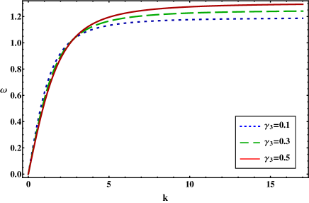
Figure 1: Plot of $\omega$ vs $k$ for different values of $\gamma_{3}$ when $\gamma_{1}=0.7$, $\gamma_{2}=0.5$, $\gamma_{4}=1.2$, and $\kappa=1.8$.

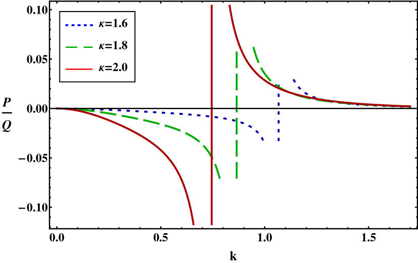
(a)

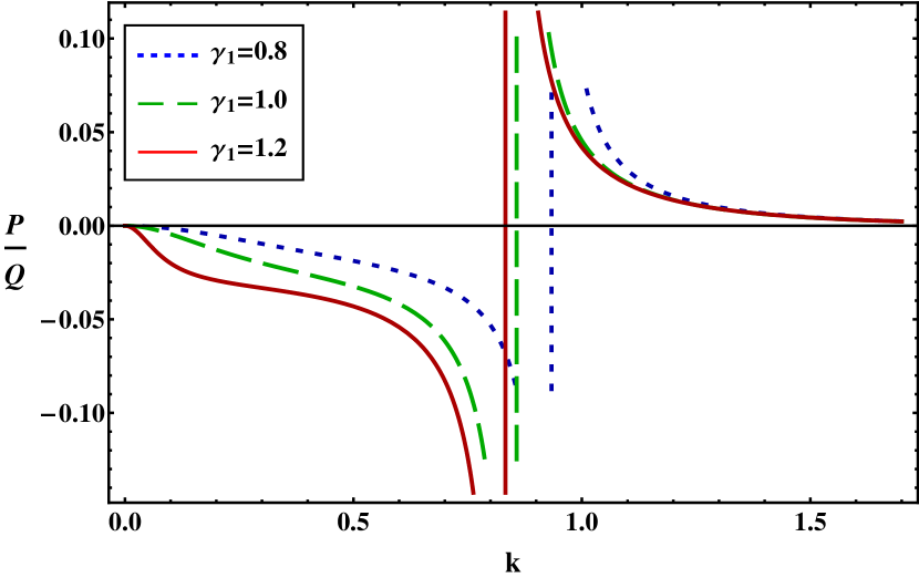
(b)

Figure 2: Showing the variation of $P/Q$ with $k$ (a) for $\kappa$ and (b) for $\gamma_{1}$, when other plasma parameters are $\gamma_{2}=0.5$, $\gamma_{3}=0.4$, and $\gamma_{4}=1.2$.

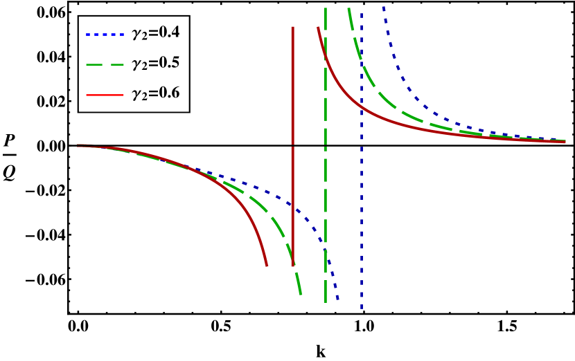
(a)

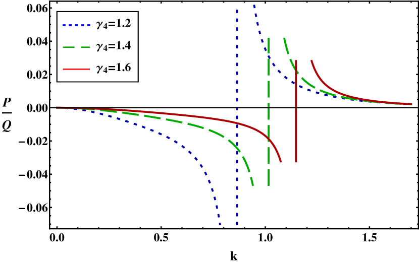
(b)

Figure 3: Showing the variation of $P/Q$ with $k$ (a) for $\gamma_{2}$ and (b) for $\gamma_{4}$, when other plasma parameters are $\gamma_{1}=0.7$, $\gamma_{3}=0.4$, and $\kappa=1.8$.

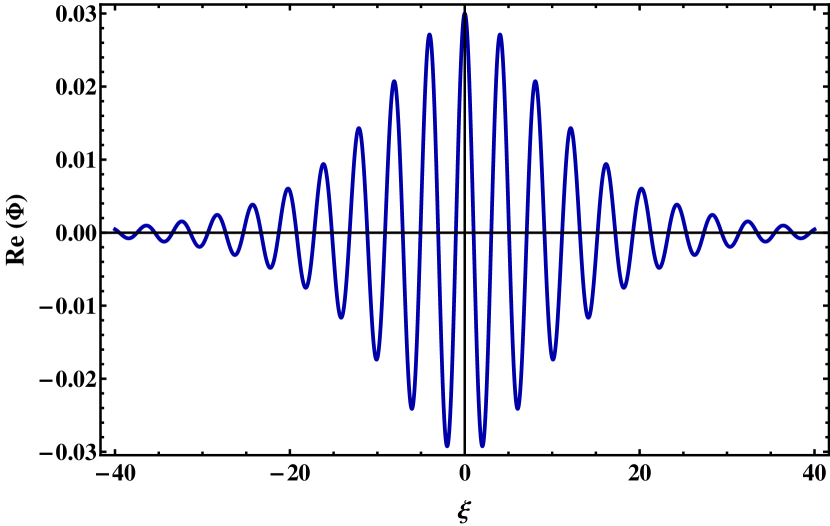
(a)

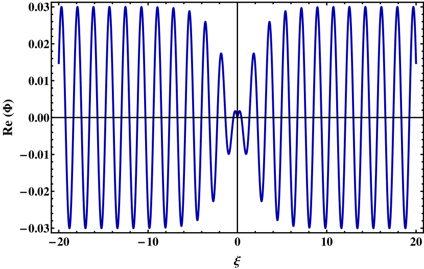
(b)

Figure 4: (a) Bright envelope solitons for $k=1.0$ and (b) dark envelope solitons for $k=0.2$, when other plasma parameters are $\tau=0$, $\psi_{0}=0.0009$, $U=0.3$, $\Omega_{0}=0.4$, $\kappa=1.8$, $\gamma_{1}=0.7$, $\gamma_{2}=0.5$, $\gamma_{3}=0.4$, and $\gamma_{4}=1.2$.

4 Modulational instability and envelope solitons

When $P$ and $Q$ are opposite sign then they offer a modulationally stable region for IAWs and allow to generate electrostatic dark envelope solitions. On the other hand, when both $P$ and $Q$ are of the same sign then they offer a modulationally unstable region for IAWs and allow to generate electrostatic bright envelope solitions [17, 18, 19, 20, 21, 22, 23]. The plot of $P/Q$ against $k$ yields stable and unstable domains for the DAWs. The point, at which transition of $P/Q$ curve intersect with $k$-axis, is known as threshold or critical wave number $k$ ($=k_{c}$).

A clear idea about the effects of $\kappa$ on the stable and unstable regions for IAWs can be observed from Fig. 2(a), and the outcomes from this figure can be expressed as (i) there is a stable region (i.e., $k<k_{c}$) for IAWs in the figure, and this stable region allows to generate the electrostatic dark envelope solitons; (ii) similarly, there is a unstable region (i.e., $k>k_{c}$) for IAWs in the figure, and this unstable region allows to generate the electrostatic bright envelope solitons; (iii) the stable region for the IAWs decreases with the increase in the value of $\kappa$. The variation of $P/Q$ with $k$ for different values of $\gamma_{1}$ can be shown in Fig. 2(b) which provides the information about the effects of the mass of the positive ($m_{+}$) and negative ($m_{-}$) ions as well as their charge state of the positive ($Z_{+}$) and negative ($Z_{-}$) ions, and it is clear from this figure that (i) an increase in the value of $\gamma_{1}$ can shift the $k_{c}$ to a smaller value of $k$ while a decrease in the value of $\gamma_{1}$ can shift the $k_{c}$ to a larger value of $k$; (ii) a massive positive (negative) ion allows to generate electrostatic bright envelope solitons associated with IAWs for small (large) value of $k$ by reducing (increasing) $k_{c}$ (via $\gamma_{1}=Z_{-}m_{+}/Z_{+}m_{-}$).

Figure 3(a) indicates the deviation in the stable and unstable regions of IAWs according to the variation of $\gamma_{2}$, and it can be seen from this figure that (i) an increase in the value of $\gamma_{2}$ is responsible for a fast destabilization of the IAWs as well as allows to generate electrostatic bright envelope solitons for small value of $k$; (ii) the presence of excess super-thermal electron would reduce the $k_{c}$ to a lower value while the presence of excess inertial positive ion would lead the $k_{c}$ to a higher value for a constant value of $Z_{+}$; (iii) highly dense super-thermal electrons offer bright envelope solitons (i.e., $k>k_{c}$) associated IAWs for small $k$ while excess inertial positive ions offer bright envelope solitons (i.e., $k>k_{c}$) associated IAWs for large $k$ (via $\gamma_{2}=n_{e0}/Z_{+}n_{+0}$). Figure 3(b) reflects the temperature effect of the electron and positron (via $\gamma_{4}=T_{e}/T_{p}$) in recognizing the stable and unstable regions of IAWs as well as the formation of bright and dark envelope solitons, and it is obvious from this figure that (i) the stable region for IAWs increases with increasing value of $\gamma_{4}$; (ii) the temperature of electron maximizes (minimizes) the $k_{c}$ as well as modulationally stable region of IAWs.

The bright (when $P/Q>0$) and dark (when $P/Q<0$) envelope soliton solutions, respectively, can be written as [22, 23, 9, 24, 25, 26]

$$\Phi(\xi,\tau)=\left[\psi_{0}~{}\mbox{sech}^{2}\left(\frac{\xi-U\tau}{W}\right)\right]^{\frac{1}{2}}\times\exp\left[\frac{i}{2P}\left\{U\xi+\left(\Omega_{0}-\frac{U^{2}}{2}\right)\tau\right\}\right],$$ (39)

$$\Phi(\xi,\tau)=\left[\psi_{0}~{}\mbox{tanh}^{2}\left(\frac{\xi-U\tau}{W}\right)\right]^{\frac{1}{2}}\times\exp\left[\frac{i}{2P}\left\{U\xi-\left(\frac{U^{2}}{2}-2PQ\psi_{0}\right)\tau\right\}\right],$$ (40)

where $\psi_{0}$ indicates the envelope amplitude, $U$ is the traveling speed of the localized pulse, $W$ is the pulse width which can be written as $W~{}[=(2P\psi_{0}/Q)^{1/2}]$, and $\Omega_{0}$ is the oscillating frequency for $U=0$. we have depicted bright and dark envelope solitons in Figs. 4(a) and 4(b) by numerically analyzed Eqs. (39) and (40), respectively.

5 Conclusion

The amplitude modulation of IAWs has been theoretically investigated in an unmagnetized four components PIP medium consisting of positively and negatively charged inertial ions as well as inertialess $\kappa$-distributed electrons and positrons. A NLSE, which governs the MI of IAWs and the formation of electrostatic bright and dark envelope solitons in PIP medium, is derived by using the RPM. To conclude, we hope that our results may be useful in understanding the nonlinear phenomena (viz. MI of IAWs and envelope solitons) in space PIP system (viz., upper regions of Titan’s atmosphere [1], chromosphere, solar wind, D-region ($\rm H^{+},O_{2}^{-}$) and F-region ($\rm H^{+},H^{-}$) of the Earth’s ionosphere [2], cometary comae [3, 4]) and laboratory PIP system (viz., neutral beam sources [5], plasma processing reactors [6], and Fullerene ($\rm C^{+},C^{-}$) [7, 36], etc.).

References

- [1] S. K. El-Labany, W. M. Moslem et al., Astrophys. Space Sci. 338, 3 (2012).
- [2] S. A. Elwakil, E. K. El-Shewy, and H. G. Abdelwahed, Phys. Plasmas 17, 052301 (2010).
- [3] P. H. Chaizy, H. Rème, J. A. Sauvaud et al., Nature 349, 393 (1991).
- [4] N. A. Chowdhury, A. Mannan, M. M. Hasan, and A. A. Mamun, Chaos 27, 093105 (2017).
- [5] M. Bacal and G. W. Hamilton, Phys. Rev. Lett. 42, 1538 (1979).
- [6] R. A. Gottscho and C. E. Gaebe, IEEE Trans. Plasma Sci. 14, 92 (1986).
- [7] R. Sabry, Phys. Plasmas 15, 092101 (2008).
- [8] V. M. Vasyliunas, J. Geophys. Res. 73, 2839 (1968).
- [9] S. Sultana and I. Kourakis, Plasma Phys. Control. Fusion 53, 045003 (2011).
- [10] D. K. Ghosh, P. Chatterjee, and B. Sahu, Astrophys. Space Sci. 341, 559 (2012).
- [11] P. Chatterjee and U. N. Ghosh, Eur. Phys. J. D 64, 413 (2011).
- [12] A. Saha, N. Pal, and P. Chatterjee, Phys. Plasmas 21, 102101 (2014).
- [13] S. K. El-Labany, R. Sabry, W. F. El-Taibany, and E. A. Elghmaz, Astrophys. Space Sci. 340, 77 (2012).
- [14] N. A. Chowdhury, A. Mannan, and A. A. Mamun, Phys. plasmas 24, 113701 (2017).
- [15] M. H. Rahman, A. Mannan, N. A. Chowdhury, and A. A. Mamun, Phys. Plasmas 25, 102118 (2018).
- [16] S. Jahan, N. A. Chowdhury, A. Mannan, and A. A. Mamun, Commun. Theor. Phys. 71, 327 (2019).
- [17] H. Gharaee, S. Afghah, and H. Abbasi, Phys. Plasmas 18, 032116 (2011).
- [18] N. A. Chowdhury, M. M. Hasan, A. Mannan, A. A. Mamun, Vacuum 147, 31 (2018).
- [19] H. Alinejad, M. Mahdavi, and M. Shahmansouri, Astrophys. Space Sci. 352, 571 (2014).
- [20] P. Eslami, M. Mottaghizadeh, and H. R. Pakzad, Phys. Plasmas 18, 102313 (2011).
- [21] N. Ahmed, A. Mannan, N. A. Chowdhury, and A. A. Mamun, Chaos 28, 123107 (2018).
- [22] I. Kourakis and P. K. Shukla, Phys. Plasmas 10, 3459 (2003).
- [23] I. Kourakis and P. K. Shukla, Nonlinear Proc. Geophys. 12, 407 (2005).
- [24] M. H. Rahman, N. A. Chowdhury, A. Mannan, M. Rahman, and A. A. Mamun, Chinese J. Phys. 56, 2061 (2018).
- [25] N. A. Chowdhury, A. Mannan, M. R. Hossen, and A. A. Mamun, Contrib. Plasma Phys. 58, 870 (2018).
- [26] N. A. Chowdhury, A. Mannan, M. M. Hasan, and A. A. Mamun, Plasma Phys. Rep. 45, 01 (2019).
- [27] A. E. Dubinov, I. D. Dubinova, and V. A. Gordienko, Phys. Plasmas 13, 082111 (2006).
- [28] A. E. Dubinov, S. K. Saikov, and A. P. Tsatskin, J. Exp. Theo. Phys. 112, 1051 (2011).
- [29] N. Jannat, M. Ferdousi, and A. A. Mamun, Plasma Phys. Rep. 42, 678 (2016).
- [30] E. Saberian, A. Esfandyri-Kalejahi, and M. Afsari-Ghazi, Plasma Phys. Rep. 43, 83 (2017).
- [31] I. Kourakis, A. Esfandyri-Kalejahi, M. Mehdipoor, and P. K. Shukla, Phys. Plasmas 13, 052117 (2006).
- [32] A. Esfandyri-Kalejahi, I. Kourakis, M. Mehdipoor, and P. K. Shukla, J. Phys. 39, 13817 (2006).
- [33] A. Esfandyri-Kalejahi, I. Kourakis, and P. K. Shukla, Phys. Plasmas 13, 122310 (2006).
- [34] U. M. Abdelsalam, W. M. Moslem, A. H. Khater, and P. K. Shukla, Phys. Plasmas 18, 092305 (2011).
- [35] S. K. El-Labany, E. K. El-Shewy et al., Plasma Phys. Rep. 18, 092305 (2011).
- [36] S.Khondaker et al., Contrib. Plasma Phys. e201800125. https://doi.org/10.1002/ctpp.201800125 (2019).