Leveraging the bfloat16 Artificial Intelligence Datatype For Higher-Precision Computations

Abstract

In recent years fused-multiply-add (FMA) units with lower-precision multiplications and higher-precision accumulation have proven useful in machine learning/artificial intelligence applications, most notably in training deep neural networks due to their extreme computational intensity. Compared to classical IEEE-754 32 bit (FP32) and 64 bit (FP64) arithmetic, these reduced precision arithmetic can naturally be sped up disproportional to their shortened width. The common strategy of all major hardware vendors is to aggressively further enhance their performance disproportionately. One particular FMA operation that multiplies two BF16 numbers while accumulating in FP32 has been found useful in deep learning, where BF16 is the 16-bit floating point datatype with IEEE FP32 numerical range but 8 significant bits of precision. In this paper, we examine the use this FMA unit to implement higher-precision matrix routines in terms of potential performance gain and implications on accuracy. We demonstrate how a decomposition into multiple smaller datatypes can be used to assemble a high-precision result, leveraging the higher precision accumulation of the FMA unit. We first demonstrate that computations of vector inner products and by natural extension, matrix-matrix products can be achieved by decomposing FP32 numbers in several BF16 numbers followed by appropriate computations that can accommodate the dynamic range and preserve accuracy compared to standard FP32 computations, while projecting up to 5.2$\times$ speed-up. Furthermore, we examine solution of linear equations formulated in the residual form that allows for iterative refinement. We demonstrate that the solution obtained to be comparable to those offered by FP64 under a large range of linear system condition numbers.

I Introduction

bfloat16 (BF16) is a new floating-point format [1] that is gaining traction due to its ability to work well in machine learning algorithms, in particular deep learning training. In contrast to the IEEE754-standardized 16bit (FP16) variant, BF16 does not compromise at all on range when being compared to FP32. As a reminder, FP32 numbers have 8 bits of exponent and 24 bits of mantissa (one implicit). BF16 cuts 16 bits from the 24-bit FP32 mantissa to create a 16-bit floating point datatype. In contrast FP16, roughly halves the FP32 mantissa to 10 explicit bits and has to reduce the exponent to 5 bits to fit the 16-bit datatype envelope.

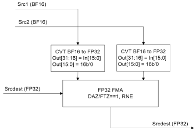
Figure 1: BF16 FMA unit as proposed in [2]. This unit is fully compatible with IEEE FP32.

Although BF16 offers less precision than FP16, it is better suited to support deep learning tasks. As shown in [3], FP16’s range is not enough to accomplish deep learning training out-of-the-box due to its limited range. BF16 does not suffer from this issue and the limited precision actually helps to generalize the learned weights in the neural net training task. In other words, lower precision can be seen as offering a built-in regularization property.

Additionally, the heart of deep learning is matrix multiplication. That means computing inner products of vectors of various length. Normally the dimensions of these vectors are pretty long: several hundreds to tens of thousands. Therefore, the community has settled on mixed-precision fused-multiply-add (FMA) hardware units. E.g. NVIDIA announced their FP16 input with FP32 output Tensorcores support in Volta and Turing GPUs and Intel has recently published their BF16 hardware numeric definition for up-coming processors code-named Cooper Lake [2]. NVIDIA did not publish the exact hardware specification, whereas Intel’s BF16 FMA is depicted in Fig. 1. The heart of this is a traditional FP32 FMA unit which can deal with BF16 numbers that are interpreted as short FP32 numbers. The key functionality is the FP32 accumulation of the unit. This means that the 16bit product’s result is fully preserved and accumulated with 24bit precision. Google’s TPU also offers BF16 multiply with FP32 accumulate, but as for NVIDIA’s Volta and Turing, the exact hardware definition is not available.

When looking at the FP16/BF16 performance specs, we can make one important observation: the number of floating point operations per second (FLOPS) provided in these formats are at least one order of magnitude higher than for FP32. E.g. Volta offers more than 120 TFLOPS of FP16 compute while only providing 15 TFLOPS of FP32 compute (both FMA). This is due to much smaller multiplier and offering the FLOPS only in form of matrix multiplication by implementing a systolic array in hardware. BF16 is expected to be even better in this respect as the mantissa is 30% shorter. Therefore one pressing question is: can this high computational performance be efficiently harvested for FP32 compute.

There is a precedent in HPC research to exploit multiple floating-point numbers combined together, often references as single-single or double-double precision [4]. This does nothing for the exponent bits, but if we consider two BF16s combined together, that yields 8 bits of exponent and 16 bits of mantissa total. And three BF16s would represent 8 bits of exponents and 24 bits of mantissa total. The first observation one might make is that this last case, a triplet of BF16s, is comparable to FP32 as we have identical range and mantissa bits. Recently such an idea was also employed for NVIDIA Tensorcores with two FP16 numbers for FFT [5]. However more mechanics are needed due to lower ranges of FP16 and only 22 bits total mantissa (if counting the implicit bits.)

In this paper, we study the numerical properties, accuracy, and performance ramifications of 3 (or 2) BF16 combined together versus FP32. Despite a similar number of exponent bits and mantissa bits, resulting algorithms will not be bitwise identical to FP32 calculations. In some cases, it will be less accurate. In some cases, it will be more accurate.

In our numeric studies, we consider the case of doing a dot product of two vectors x and y. This is the basis of a matrix-matrix multiply algorithm (GEMM), which in turn is the basis for many computations in linear algebra, as GEMM is the core routine behind the Level-3 BLAS [6] and much of LAPACK [7].

Our paper makes following contributions:

• we discuss an accumulation error analysis for the dot-product of two vectors represented as triplets of BF16 numbers. There are cases where multiplying two BF16s might yield exact, or near exact, results. This means that we often will have much greater accuracy than FP32 calculations.

• we consider the issue of “short-cuts” where we don’t consider all the bits available to us. For instance, three BF16 splitting of FP32 number will require 9 multiplication (all-to-all), but do we really need to consider lower-order terms? The least significant bits should have a minimal impact on the final result. We will show that a 6-produce version achieves acceptable accuracy.

• we analyze common BLAS and LAPACK kernels, namely SGEMM and SGETRF using our combined datatype. We focus on matrices of both small and large exponential range.

• we consider performance implications: asymptotically a 6-product version has six times as much work compared to GEMM in FP32. Depending on the factor improvement of BF16 GEMM over FP32 GEMM, a closer look at the accuracy and performance ramifications is not only interesting, but justified, potentially offering up to 5.2$\times$ speed-up.

• to complete our work, we also investigate how BF16 compares to FP16 when being used in one-sided decomposition which are sped-up by iterative refinement. Here we can conclude that in general case BF16 may not be enough, but for diagonally-dominant matrices its performance is comparable to FP16.

II Combined Lower Precision Datatypes And Their Application to BLAS and LAPACK Routines

This sections covers how we decompose FP32 numbers into multiple BF16 numbers and derives error bounds for dot-product computations using this type. We also discuss how we can skip lower order terms while maintaining FP32 comparable accuracy.

II-A Decomposition of a FP32 number into multiple BF16 numbers

We use the notation ${\cal F}_{32}$ and ${\cal B}_{16}$ to denote that set of reals number representable in FP32 and BF16, respectively. Lets assume that $a$ is a ${\cal F}_{32}$ number and it is stored into 3 ${\cal B}_{16}$: ${b}^{({0})}$, ${b}^{({1})}$, and ${b}^{({2})}$. $({\cal F}_{32})$ and $({\cal B}_{16})$ shall denote the conversion operator to the respective type. We assign these values as follows:

$${b}^{({0})}= ({\cal B}_{16})a$$

$${b}^{({1})}= ({\cal B}_{16})(({\cal F}_{32})(a-({\cal F}_{32}){b}^{({0})}))$$

$${b}^{({2})}= ({\cal B}_{16})(({\cal F}_{32})(a-({\cal F}_{32}){b}^{({0})}–({\cal F}_{32}){b}^{({1})}))$$

One can imagine that $a$ is an approximation of $({\cal F}_{32}){b}^{({0})}+({\cal F}_{32}){b}^{({1})}+({\cal F}_{32}){b}^{({2})}$. Adding two triplets together has 3 times the number of adds. Multiplying two triplets together has 9 times the number of multiplies, not to mention extra adds as well, which are free when using FMA units.

II-B Dot Product Notation

Given two vectors $\mathbf{x},\mathbf{y}\in\mathbb{R}^{n}$ both of which representable exactly in IEEE single precision format, the goal is to compute the inner product $\mathbf{x}^{T}\mathbf{y}$. The reference is the standard computation in FP32 using FMA, that is, one rounding error in each accumulation. What we want to explore is to use BF16 to compute the inner product. The basic idea is that each FP32 representable value can be decomposed exactly into the unevaluated sum of three BF16 representable numbers and thus the inner product in question is expressible in 9 inner products involving vectors of BF16 representable values.

Here is the basic set up:

$$\mathbf{x} =[x_{1},x_{2},\ldots,x_{n}]^{T}\in{\cal F}_{32}^{n}$$

$$\mathbf{y} =[y_{1},y_{2},\ldots,y_{n}]^{T}\in{\cal F}_{32}^{n}$$

$${\mathbf{x}}^{({i})} =[{x_{1}}^{({i})},{x_{2}}^{({i})},\ldots,{x_{n}}^{({i})}]^{T}\in{\cal B}_{16}^{n},\quad i=0,1,2$$

$${\mathbf{y}}^{({i})} =[{y_{1}}^{({i})},{y_{2}}^{({i})},\ldots,{y_{n}}^{({i})}]^{T}\in{\cal B}_{16}^{n},\quad i=0,1,2$$

$$z =\mathbf{x}^{T}\mathbf{y},\quad\hat{{z}}=|\mathbf{x}|^{T}|\mathbf{y}|=\sum_{\ell=1}^{n}|x_{\ell}y_{\ell}|$$

$${z}^{({i,j})} ={{\mathbf{x}}^{({i})}}^{T}{\mathbf{y}}^{({j})},\quad{\hat{{z}}}^{({i,j})}=\sum_{\ell=1}^{n}|{x_{\ell}}^{({i})}{y_{\ell}}^{({j})}|,\quad 0\leq i,j\leq 2$$

$$\varepsilon_{f} =2^{-24},\quad\varepsilon_{b}=2^{-8}$$

$$\gamma_{f,{k}} =\frac{k\varepsilon_{f}}{1-k\varepsilon_{f}},\quad\gamma_{b,{k}}=\frac{k\varepsilon_{b}}{1-k\varepsilon_{b}}$$

II-C Basic Bounds on Single Precision

The standard computation in FP32 is as follows:

$Z\leftarrow 0$
   For $\ell=1,2,\ldots,n$:
         $Z\leftarrow{\tt FMA}(x_{\ell},y_{\ell},Z)\\$    End

The error bound is standard in this case, namely

$$|Z-z|\leq\gamma_{f,{n}}\hat{{z}}$$

That is, the absolute error is roughly $n$ rounding errors times the inner product with the absolute value of the vectors. So the relative error with respect to $z$ is roughly $n$ rounding errors if there is not much cancellation. Indeed, the ratio $\hat{{z}}/|z|\geq 1$ is usually called the condition number in this case. So the rest of the document tries to derive similar upper bounds on the error when we use various summation procedure utilizing FMA accumulation to first compute the ${z}^{({i,j})}$s, followed by summation.

II-D Error Analysis for combined BF16 Datatypes

The following quantities are the relevant components, although various specific inner product computation may use only a subset of these quantities.

For each $i,j$, $0\leq i,j\leq 2$, we compute in FP32 precision the nine partial inner products.

${Z}^{({i,j})}\leftarrow 0$
   For $\ell=1,2,\ldots,n$:
         ${Z}^{({i,j})}\leftarrow{\tt FMA}({x_{\ell}}^{({i})},{y_{\ell}}^{({j})},{Z}^{({i,j})})$
   End

Add the partial products of “equal levels”. In FP32 arithmetic do the following

${Z}^{({0})}\leftarrow{Z}^{({0,0})}$
   ${Z}^{({1})}\leftarrow{Z}^{({0,1})}+{Z}^{({1,0})}$
   ${Z}^{({2})}\leftarrow{Z}^{({0,2})}+({Z}^{({1,1})}+{Z}^{({2,0})})$
   ${Z}^{({3})}\leftarrow{Z}^{({1,2})}+{Z}^{({2,1})}$
   ${Z}^{({4})}\leftarrow{Z}^{({2,2})}$
We use the lower case $z$ to denote the corresponding exact values. For example ${z}^{({2})}={z}^{({0,2})}+{z}^{({1,1})}+{z}^{({2,0})}$ and ${z}^{({1,1})}=\sum_{\ell=1}^{n}{x_{\ell}}^{({1})}{y_{\ell}}^{({1})}$. A simple sum that offers close-to-FP32 accuracy is to compute in FP32 arithmetic

$$Z_{2}\leftarrow{Z}^{({0})}+({Z}^{({1})}+{Z}^{({2})})$$

A sum that might be able to offer higher accuracy than FP32 is to compute in FP32 arithmetic

$$Z_{3}\leftarrow{Z}^{({0})}+({Z}^{({1})}+({Z}^{({2})}+{Z}^{({3})}))$$

II-E General error bound on $Z_{2}$

Recall that a recursive sum $S$, computed in FP32, of $n$ items whose exact sum is $s$ satisfies $|S-s|\leq\gamma_{f,{n}}\hat{{s}}$. Note also that $\gamma_{f,{m}}+\gamma_{f,{n}}\leq\gamma_{f,{n+m}}$. Applying this we obtain

$$|{Z}^{({i,j})}-{z}^{({i,j})}| \leq\gamma_{f,{n}}\varepsilon_{b}^{i+j}\hat{{z}}$$

$$|{Z}^{({i,j})}| \leq(1+\gamma_{f,{n}})\varepsilon_{b}^{i+j}\hat{{z}}\leq 1.01\varepsilon_{b}^{i+j}\hat{{z}}$$

Similarly

$$|{Z}^{({0})}-{z}^{({0})}| \leq\gamma_{f,{n}}\hat{{z}}$$

$$|{Z}^{({1})}-({Z}^{({0,1})}+{Z}^{({1,0})}| \leq\gamma_{f,{1}}(|{Z}^{({0,1})}|+|{Z}^{({1,0})}|)$$

$$\leq 2.02\gamma_{f,{1}}\varepsilon_{b}$$

$$|{Z}^{({2})}-({Z}^{({0,2})}+{Z}^{({1,1})}+{Z}^{({2,0})})| \leq 3.03\gamma_{f,{2}}\varepsilon_{b}^{2}$$

Consequently, we have

$$\sum_{i=0}^{2}|{Z}^{({i})}-{z}^{({i})}| \leq(\gamma_{f,{n}}+2.02\gamma_{f,{1}}\varepsilon_{f}+3.03\gamma_{f,{2}}\varepsilon_{b}^{2})\hat{{z}}$$

$$\leq 1.01\gamma_{f,{n}}\hat{{z}}$$

We can now estimate $|Z_{2}-z|$ which is the error we get in computing the inner product using BF16 and gather only up to the second order partial inner products. The error consist of truncation error in ignoring a couple of the partial inner products and also the rounding errors in computing $Z_{2}$.

$$|Z_{2}-z| \leq|Z_{2}-({z}^{({0})}+{z}^{({1})}+{z}^{({2})})|+|{z}^{({3})}+{z}^{({4})}|$$

$$\leq|Z_{2}-({z}^{({0})}+{z}^{({1})}+{z}^{({2})})|+1.01\varepsilon_{b}^{3}\hat{{z}}$$

$$\leq|Z_{2}-({Z}^{({0})}+{Z}^{({1})}+{Z}^{({2})})|$$

$$\hskip 8.61108pt+\sum_{i=0}^{2}|{Z}^{({i})}-{z}^{({i})}|+1.01\varepsilon_{b}^{3}\hat{{z}}$$

$$\leq\gamma_{f,{2}}\sum_{i=0}^{2}|{Z}^{({i})}|+1.01\gamma_{f,{n}}\hat{{z}}+1.01\varepsilon_{b}^{3}\hat{{z}}$$

$$\leq 1.01(\gamma_{f,{n+2}}+\varepsilon_{f}^{3})\hat{{z}}.$$

The above shows that in general the worst case bound on using BF16 is slightly worse than using FP32. This cannot be corrected by using more terms as the factor $\gamma_{f,{n+1}}$ is dominant, slightly worse than $\gamma_{f,{n}}$. There is a special case, however, in which $Z_{2}$ can be significantly more accurate. This is the situation when ${Z}^{({0})}={z}^{({0})}$. That is, the computation of $\sum_{\ell=1}^{n}{x_{\ell}}^{({0})}{y_{\ell}}^{({0})}$ is exact, This is quite possible as each product ${x_{\ell}}^{({0})}{y_{\ell}}^{({0})}$ only has at most 16 significant bits and that we are accumulating into an FP32 number, which holds 24 significant bits. The exact sum’s magnitude is clearly less than $n\max_{\ell}|{x_{\ell}}^{({0})}{y_{\ell}}^{({0})}|$. As long as the least significant bit position of $\min_{\ell}|{x_{\ell}}^{({0})}{y_{\ell}}^{({0})}|$ is not farther than 23 bits away, the sum will be exact. A mathematical relationship that implies this situation is

$$\lceil\log_{2}(1.01\,\max_{\ell}|x_{\ell}y_{\ell}|)\rceil-23\leq\lceil\log_{2}(0.99\,\min_{\ell}|x_{\ell}y_{\ell}|)\rceil-15$$

If this holds, we have ${Z}^{({0})}-{z}^{({0})}=0$ and the previous error bound reduces to

$$|Z_{2}-z|\leq 1.01\,(\gamma_{f,{2}}+\varepsilon_{b}^{3})\hat{{z}}\leq 1.01\,\gamma_{f,{3}}\hat{{z}}$$

II-F Worse Case Error for combined BF16 Datatypes

The worst error that can occur with this method is when the original FP32 number, $a$, is very close to zero, that is contains a large negative exponent near the exponent boundary of FP32 (like -126, since -127 is reserved for denormals). What happens then is the conversion from FP32 to BF16 for the first number will be alright (${b}^{({0})}=({\cal B}_{16})a$), but the second BF16 number ${b}^{({1})}$ will be with an exponent shifted left by 8, and the third BF16 number ${b}^{({2})}$ will be with an exponent shifted left by 16. In which case, ${b}^{({1})}={b}^{({2})}=0.0$. Let’s assume that $a$ has many nonzero bits in the mantissa, but all but one of them are in positions 0-15. If that’s the case, then all those bits will be lost when we determine ${b}^{({1})}={n}^{({2})}=0.0$.

The error in this case is the worst because $a$ and ${b}^{({0})}$ will only have 8 mantissa bits in common, and so any product that uses $a$ might only have 2-3 digits of accuracy and the rest of the product will be off. Again, this is the worst case scenario and only seems to happen when the exponents are large and negative. As long as the exponent of $a$ is at least no smaller than -110, then we can form ${b}^{({1})}$ and ${b}^{({2})}$ within the FP32 threshold. So a ”bad” number to try with this method would probably have a small value in exponent bit fields 30-23 (like 00000001), so that the exponent bias pushes this to an extreme negative number, and perhaps a 1 in the bit field 16, and zeros in 22-17, and then bits 0-15 are all 1s, like $\approx 1.1939\cdot 10^{-38}$.

For this reason, routines in LAPACK like DLATRS which depend on scaling and shifting triangular matrices to prevent denormals often keep track of the magnitude of numbers, avoiding the biggest and smallest by scaling the data. They typically use constants close to the exponent range. To fully make use of such a routine, it’d be wise to use a pretend range of $[-110,127]$.

II-G Possible Shortcuts when using three-way and two-way BF16 combined Datatypes

Following the previous general error analysis of Sec. II-E, we can now have a more detailed look on saving operations. Because the number of significant bits of BF16 are 8, we expect that $|{a}^{({1})}|<=2^{-8}|{a}^{({0})}|$ and $|{a}^{({2})}|<=2^{-16}|{a}^{({0})}|$. While we won’t know in general how the $a$-terms compare with the $b$-terms, we do know this puts these terms into five separate bins with ${a}^{({0})}\cdot{b}^{({0})}$ as our primary, most significant term and in its own bin. The other four bins are:

$$|{a}^{({0})}\cdot{b}^{({1})}|,|{a}^{({1})}\cdot{b}^{({0})}|\leq 2^{-8}|{a}^{({0})}\cdot{b}^{({0})}|$$

$$|{a}^{({1})}\cdot{b}^{({1})}|,|{a}^{({0})}\cdot{b}^{({2})}|,|{a}^{({2})}\cdot{b}^{({0})}|\leq 2^{-16}|{a}^{({0})}\cdot{b}^{({0})}|$$

$$|{a}^{({1})}\cdot{b}^{({2})}|,|{a}^{({2})}\cdot{b}^{({1})}|\leq 2^{-24}|{a}^{({0})}\cdot{b}^{({0})}|$$

$$|{a}^{({2})}\cdot{b}^{({2})}|\leq 2^{-32}|{a}^{({0})}\cdot{b}^{({0})}|$$

Let’s define $E={a}^{({1})}\cdot{b}^{({2})}+{a}^{({2})}\cdot{b}^{({1})}+{a}^{({2})}\cdot{b}^{({2})}$. This $E$ term is the difference between computing our triplet with 6 multiplies with only the most significant bins, and 9 multiplies with all bins. The first observation is while $|{a}^{({1})}|<=|{a}^{({0})}|/256$, in which case equality can and does sometimes happen, it is usually a smaller term. But first, plugging in this observation into the above equation for $E$ simplifies to $E\leq|c*{a}^{({0})}{b}^{({0})}|\cdot 2^{-23}$ where c=${513/512}.$

We start by making our bounds on $|{a}^{({0})}|$ and $|{b}^{({0})}|$ more rigorous. If we assume that exponents are larger than $-110$ (see the previous section for why), and the numbers are uniformly distributed in a given range, we can show that the expected average value of $|{a}^{({1})}|\approx|{a}^{({0})}/768|.$ Note that $d*|{a}^{({0})}|<|{a}^{({1})}|$ for some $d$. In particular, $d$ is in $(2^{-9},2^{-8})$ with probability 1/2 if we assume a uniformly distributed range of data (we assume that the relevant bit can either be 0 or 1 if the data is uniformly distributed.) If the relevant bit isn’t helpful here, we can assume the next relevant bit will be and $d$ will lie in $(2^{-10},2^{-9})$ with probability 1/4. And $d$ will lie in $(2^{-11},2^{-10})$ with probability 1/8. Also note that the mantissa of $|{a}^{({i})}|$ is uniformly in $[1,2)$, so we can cut our averages by a factor of 2. In particular, we have a series $2\cdot(\frac{1}{2}+\frac{1}{4}\frac{1}{2}+\frac{1}{8}\frac{1}{4}+\cdots)=\frac{1}{3}$, so in fact, on average, $|{a}^{({1})}|\approx|{a}^{({0})}/768|.$ We can do a similar analysis and show that $|{a}^{({2})}|\approx|{a}^{({0})}/768^{2}|.$

Now we see that, on average, $|E|\approx|{a}^{({0})}{b}^{({0})}|\cdot c$ where $c\approx 4.412e-9.$ So while in the worst case some of these 3 extra terms might be important, on the average they don’t matter.

This suggests some immediate short-cuts as well as ordering. That is, the terms should be added in the reverse order, so that the smallest terms come first. One can’t take the time to test whether $|{a}^{({0})}\cdot{b}^{({1})}|<=|{a}^{({1})}\cdot{b}^{({0})}|$ but we do know that terms in the separate bins have the above relation. We also know that since three BF16s can only keep track of 24 implicit bits, it might not be worthwhile to compute the terms in the last two bins, saving some work. That doesn’t mean it won’t be worthwhile, however. For instance, consider a case like x=0.57892173110418099213 and y=-7447.6596637651937272. Because y is so much larger than x, the $|{a}^{({1})}\cdot{b}^{({2})}|$ is significant even though it’s in the $2^{-24}$ bin. And in this case, it’s necessary to compute that product if we want the BF16x3 error to be less than the real*8 error, which means computing at least 7 products instead of just 6. Nevertheless, if we assume that the terms are equal in magnitude, one might expect the values each bin to be roughly equal, and then all things considered, the last two bins are not necessary. That is, if the input values are close enough, one can mimic single precision accuracy just by first adding the terms in the $2^{-16}$ bin, then the terms in the $2^{-8}$ bin, and finally add that result to our most significant term ${a}^{({0})}\cdot{b}^{({0})}$.

The same idea can be applied if we wish to use a pair of BF16s instead of a triplet. Namely, we can skip all three terms in the $2^{-16}$ bin. But again, this is only when we assume that the all these terms are relatively the same in magnitude. There’s no precise way to know in advance that skipping terms won’t be marginally bad. All we can know is that terms satisfy the above equations, to we have an handle on the worse potential error that could arrive.

This suggests that if have a single BF16, we need to do a single multiply: ${a}^{({0})}\cdot{b}^{({0})}$. If we have two BF16s, we need to do two additional multiplications (or three total) with the two products in the $2^{-8}$ bin. If we have three BF16s, we need to do another three additional multiplications (or six total) with the three products in the $2^{-16}$ bin. In all cases, the bins should be added from smallest to largest. This is summarized in the following table.

Number of BF16s	Number of Implicit Multiplies
1	1
2	3
3	6

Another potential short-cut we’ve explored is assuming the two numbers have a different number of splits. That is, suppose we multiply $({a}^{({0})},{a}^{({1})})\times({b}^{({0})},{b}^{({1})},{b}^{({2})})$. To get maximum accuracy, one might expect to do five multiplies, taking only the ${a}^{({1})},{a}^{({1})}$ and ${a}^{({0})},{a}^{({2})}$ terms from the $2^{-16}$ bin. However, we really need to assume that ${a}^{({1})}~{}=0$ and dropping this term is okay, because neither of those two terms we in use in the $2^{-16}$ bin will be sufficient to approximate FP32 accuracy otherwise.

Note, all of these combinations open up an avenue for novel performance optimization techniques in numeric applications, in particular dense linear algebra. For both operands, often matrices $A$ and $B$ we can now employ different decompositions into lower precision datatypes to fulfill the application’s need for accuracy and balance it with execution speed.

III Speeding Up One-Sided Solvers With low-precision Datatypes using Residual Formulation

Mixed precision high performance computing is showing up more and more [8].

One key benefit in this paper is the combining of low-precision data types in order to get higher precision. But there’s another benefit, and it’s historically what most people think of first with regard to lower precision, because it’s what has been known about for years. Namely, for some problems that contain an obvious residual equation, one can first solve the problem in lower precision, and hopefully faster, and then iteratively refine on higher precision. If it works, and it may not, the final answer will be just as accurate as if higher precision had been used the entire time. And if the bulk of the operations are in lower precision, hopefully the computation will also run faster.

This is most commonly done when solving a system of equations [9], like $Ax=b$ using Gaussian Elimination in a $LU$ factorization. It’s a common thread in numerical analysis to first solve the problem in lower precision, then compute the residual in higher precision, $r=A*x-b$, and use the results from the lower precision solver to solve the updated system $Ay=r$ (just use the $LU$ factorization, but do the solve in a higher precision like FP64 as well), and then update $x$ with $x+y$. Only the cubic work of the initial $LU$ factorization should be done in the lower precision: all the other steps, which are all quadratic instead of cubic, should be done in the higher precision. Asymptotically, the cubic lower-precision work should dominate the time, but the accuracy (if the technique works) should approach FP64. This method is called Iterative Refinement on $LU$, and tends to break down when the matrix condition number is large compared to the machine epsilon of the $LU$ work. That is, for a fixed matrix condition range, the method will tend to work more often for FP32 than FP16, and more often for FP16 than BF16.

In some cases, researchers have found that combining Iterative Refinement with an Iterative Solver like GMRES [10][11] is also beneficial, especially when the base precision is very low because the odds are that the matrix may have too high a condition number to work otherwise.

IV Experimental Results

IV-A SGEMM and SGETRF using combined BF16 Datatypes

We did a complete GEMM (GEneral Matrix-matrix Multiply) implementation which starts with FP32 data and behind the scenes converts it into one to three bfloat16 matrices and then does one to nine products with these matrices and adds it all up again. We also experimented with iterative refinement for LU, comparing FP32, with FP16 and bfloat16.

For our GEMM testing, we wanted to test three different use cases. First, just the simple case where the exponent range is small because all the numbers are within a close range (like [-1,1].) Second, where the exponent range is huge because the exponents are randomly chosen bits as well as the mantissa bits- in this case, we want numbers arbitrarily close to zero or arbitrarily close to Inf or -Inf. Third, a more ”medium” case, where we assign the exponent range to be a Gaussian distribution so that the exponents can sometimes be large, but most of the time they are small and reasonable, so we see a case where the exponents can vary, just not likely. Our theoretical understanding suggests that the small range case should do best for BF16s, and that some of the cases where the range is large shouldn’t go as well as it did in single precision. This is precisely what we find.

Figure 2 computes the ”baseline” result via DGEMM (real*8 GEMM), and computes the relative error of that versus four different methods: using a pair of BF16s and three products, using Intel Math Kernel Library’s (Intel MKL [12]) SGEMM which is a FP32 general matrix-matrix multiply, using a triplet of BF16s and six products and adding those results together in FP32, and the same as the last but adding the final results together in FP64. Unlike the next experiment, this was only for a narrow range of data [-1,1]. The results are as we expected, and the order of accuracy was the order stated here.

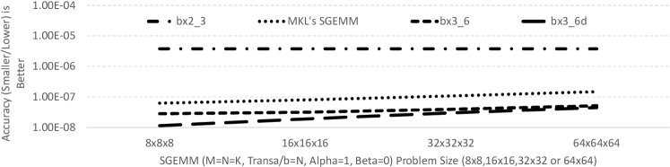
Figure 2: Various GEMM ($C=A\times B$) average relative error vs. DGEMM ($\left\|A\times B-\text{DGEMM}\right\|_{F}/\left\|\text{DGEMM}\right\|_{F}$) over 1000 runs compared to original fp64 data in [-1.0,1.0] range with drand48() randomization. bxA_B[d] means breaking each matrix up into A bfloat16 matrices, doing B products. Optionally, collect the final answer with ”d” (double precision) or not.

Figure 3 computes the ”baseline” result using FP64 DGEMM (real*8 GEMM), and computes the relative error of that versus either SGEMM or a triplet of BF16s done with six products. We only show the relative error because we have used special generation to uniformly create arbitrary exponents, so the absolute errors were sometimes huge (over $10^{20}$.) With this wide range of exponents, SGEMM actually did better (marginally) over the BF16s, but it’s still very comparable.

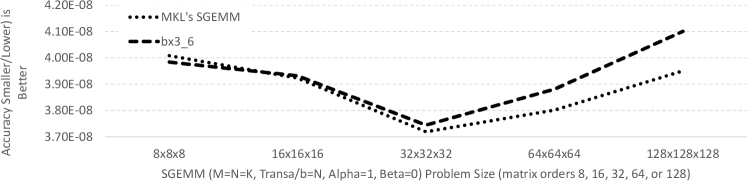
Figure 3: Same as Fig. 2, but with maximal exponent distribution (huge range).

Figure 3 exaggerates the variance, and looking closely at the vertical axis, one sees that both methods are nearly identical even when the exponent range of the data is huge.

Finally, our last GEMM case study is when the exponents have a Gaussian distribution instead of a Uniform distribution. In this case, the exponent bits were set via calling the Vector Statistical Library with ”VSL RNG METHOD GAUSSIAN BOXMULLER”) in Intel MKL[12]. So the exponents could be wide, but statistically that was unlikely, to give us more of a medium range exponent distribution as opposed to the last two examples. Again, the SGEMM and BF16 results were separately compared against DGEMM’s answer like the other two cases. Figure 4 contains these results.

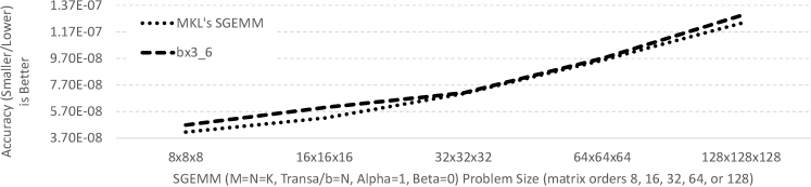
Figure 4: Same as Fig. 2, but with Gaussian exponent distribution (medium range).

In Figure  4, we see that this technique appears on average worse than SGEMM results, however the gap seems to be smaller than the wide-range case in Figure  3.

The next curve in Figure 5 was one doing an entire FP32 LU decomposition (Gaussian Elimination), in one case using SGETRF ([10]) from Intel(R) MKL (which is based on FP32 GEMM) and in the other case using a SGETRF based on triplets of BF16s and six products. Because this curve shows both small range data and large range data, we simply things just by showing the ratio of the relative errors. In every case, the triplet of BF16s was more accurate. The comparison points were results from DGETRF on the same input data.

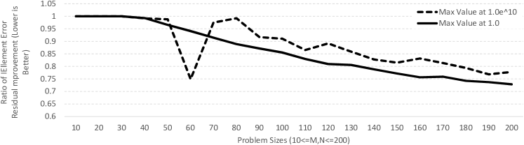
Figure 5: SGETRF vs BFLOAT16x3_6 LU Decomposition: Element errors average improvement over a 100 runs for $N\times N$ square matrices with an extremely large range $[-1.0^{10},1.0^{10}]$ and matrices with a small range $[-1.0,1.0]$

IV-B Iterative Refinement

For iterative refinement on solutions to $Ax=b$ with LU, using lower precision tends to work only for well-conditioned matrices, where the lower the precision, the more stringent conditioning is needed.

We ran 100 tests for unsymmetric dense matrices of order 50, setting the condition number and using a residual tolerance of $cond(A)*eps$. When the condition number grows, it appears that using a single bfloat16 (as opposed to the triplet discussed elsewhere) instead of FP32 gets more and more risky.

Precision	Condition #	% Converged	Ave. iterations
FP32	10	100	3.47
BF16	10	45	39.3556
FP16	10	90	16.2667
FP32	100	100	2.67
BF16	100	32	41.125
FP16	100	91	16.989
FP32	1000	100	2.49
BF16	1000	29	47.0345
FP16	1000	89	19.4831
FP32	10000	100	2.39
BF16	10000	21	48.4286
FP16	10000	91	13.5604

For row and column diagonally dominant unsymmetric matrices trying to solve $Ax=b$, one can also apply GMRES instead of iterative refinement, and use the LU decomposition in the lower precision from the last table as a pre-conditioner. We used the same tolerance as before and again 100 tests, but this time varied the sizes $n$ of the matrices instead of the condition number.

Precision	n	% Converged	Ave. iterations
FP32	10	100	2.0
BF16	10	100	6.59
FP16	10	100	4.24
FP32	50	100	2.0
BF16	50	100	7.0
FP16	50	100	5.0
FP32	100	100	2.0
BF16	100	100	7.0
FP16	100	100	5.0

We see that if the matrix is diagonally dominant, then using GMRES with the LU as a pre-conditioner allows for faster convergence and the method is more reliable.

V Performance Ramifications

We can only estimate performance at this early stage or rely on data reported on NVIDIA hardware with FP16 inputs, but not BF16 as bare-metal programmable BF16 hardware is not yet available. Timing is broken down into three parts: the conversion of data into BF16 parts (which has $N^{2}$ complexity for SGEMM), the products involved in the computation (which has $N^{3}$ complexity for SGEMM), and the final additions in the end to get the final answer (which are free as we assume FMA hardware and we chain the products). While we studied the accuracy of the SGEMM and SGETRF, the target goal is accelerating mainly all compute bound dense linear algebra functions in BLAS and LAPACK. Therefore, the aforementioned complexities are always true and we can assume that the splitting can be hidden behind the computations on modern out-of-order/threaded hardware. That means the middle step, the low precision partial matrix multiplications will dominate.

We know today that NVIDIA Volta has 10x more FLOPS in FP16 and it would be even higher with BF16. The area of FP-FMA is dominated by the multiplier as it roughly grows squared with mantissa size (and therefore also consumes a lot of power). That means this area can be approximated for FP32 as $24^{2}=576$ area-units where as BF16 requires only $8^{2}=64$ area-units. So BF16 is roughly 10$\times$ smaller using this first order approximation. Additionally, machine learning pushes the hardware vendors to implement dataflow engines (e.g. NVIDIA’s Tensorcores or Google’s TPU), also know as systolic arrays, for efficient matrix computations with dense FLOPS. Therefore we can see that 8-32$\times$ more FLOPS than the classic FP32 FLOPS within the same silicon area are possible for the right matrix computations.

The presented approached matches FP32 accuracy for important dense linear algebra routines with 6$\times$ more low-precision computations. This now opens a wide range of optimization opportunities for hardware vendors. First FP32-like dense linear algebra computation can be several times faster (when splitting can be hidden):

BF16 density over FP32	projected Speed-Up over FP32
8	$\leq 1.3=8/6$
16	$\leq 2.7=16/6$
32	$\leq 5.2=32/6$

The performance results in [5] show that the assumptions made here are correct. Similar Speed-Ups are also possible in iterative refinement scenarios [10].

Apart from having faster “FP32” on general purpose hardware such as CPUs and/or GPUs, it also means that deep learning optimized hardware, such as Google’s TPU could be efficiently used for classic HPC which only requires FP32. Only the support for splitting a FP32 number into multiple BF16 needs to be provided. There is no need for native FP32 FMA units, a mixed precision BF16-FP32 FMA unit is sufficient. People have been proposing using mixed precision to refine other problems like eigenvalue problems for years such as in [13]. More recently, there has been success with FP32 Eigenvalue solvers which are compute intensive and are the bottleneck in quantum chemistry problems[14]. These applications consume a huge fraction of large super-computers. Using the presented approach, we can use BF16 hardware without FP32 support for computation with single precision comparable accuracy.

VI Conclusions

Lower precision units like BF16 and FP16 are starting to appear with accelerated performance due to machine learning pushes. Normally, FP32 is twice as fast as FP64, but a smaller precision may widen that performance gap. This means more scientists will wish to exploit the faster calculations. We expect BF16/FP16 systolic arrays to provide 8-32$\times$ more compute potential than a classic FP32 vector compute engine.

Multiple combined BF16 have comparable accuracy (possibly better) when compared to FP32 and if a matrix-multiply can be implemented fast in terms of BF16, then it can be faster alternative to FP32’s matrix-multiply (SGEMM) as well. We have shown a line of sight to up to 5.2$\times$ faster dense linear algebra computations. Furthermore, nearly every processor is designed with FP32 these days, but this opens the door to an alternative; namely, if the processor has a fast BF16 or FP16 unit already, it may be able to emulate a lot of FP32 work, without providing extra FP32 FMA hardware. This alternative is beneficial for deep learning optimized hardware.

Mixed precision computation such as iterative refinement is a surging area of research because scientists will want to exploit a much faster lower precision. If the bulk of the work can be done faster, then perhaps the overall problem can be done faster.

In general, people used to think “less precision per element” means less overall accuracy. This paper shows that folly in that thinking. Not only can, in some cases, a smaller precision unit be combined to achieve higher accuracy, but also refinement techniques can be developed that ultimately converge to higher accuracy. Since these lower precision units allow for much denser packing on silicon, classic higher precision compute units can be outperformed performance-wise while still delivering high precision numeric results.

References

- [1] “Tensorflow development summit,” March 30 2018.
- [2] BFLOAT16 – Hardware Numerics Definition. Santa Clara, USA: Intel Corporation, 2018.
- [3] P. Micikevicius, S. Narang, J. Alben, G. F. Diamos, E. Elsen, D. García, B. Ginsburg, M. Houston, O. Kuchaiev, G. Venkatesh, and H. Wu, “Mixed precision training,” CoRR, vol. abs/1710.03740, 2017.
- [4] D. H. B. Yozo Hida, Xiaoye S Li, “Library for double-double and quad-double arithmetic,” 2007.
- [5] X. Cheng, A. Sorna, E. D’Azevedo, K. Wong, and S. Tomov, “Accelerating 2d fft: Exploit gpu tensor cores through mixed-precision,” 2018.
- [6] J. Dongarra, J. D. Croz, S. Hammarling, and I. Duff, “A set of level 3 basic linear algebra subprograms,” 1990.
- [7] E. Anderson, Z. Bai, C. Bischof, J. Demmel, J. Dongarra, J. D. Croz, A. Greenbaum, S. Hammarling, A. McKenney, and D. Sorenson, LAPACK User’s Guide. Philadelphia, PA: SIAM Publications, 1992.
- [8] I. Yamazaki et al., “Mixed-precision cholesky qr factorization and its case studies on multicore cpu with multiple gpus,” 2015, sIAM J. Sci. Comput., Volume 37, Issue 3, C307–C330.
- [9] E. Carson and N. Higham, “A new analysis of iterative refinement and its application to accurate solution of ill-conditioned sparse linear systems,” 2017, sIAM J. SCI. COMPUT. Vol. 39, No. 6, pp. A2834–A2856.
- [10] A. Haidar, S. Tomov, J. Dongarra, and N. J. Higham, “Harnessing gpu tensor cores for fast fp16 arithmetic to speed up mixed-precision iterative refinement solvers,” 2018.
- [11] Barrett and B. et al, Templates for the Solution of Linear Systems: Building Blocks for Iterative Methods. SIAM Publications, 1993.
- [12] Intel Math Kernel Library. Reference Manual. Santa Clara, USA: Intel Corporation, iSBN 630813-054US.
- [13] J. Dongarra, C. Moler, and J. Wilkinson, “Improving the accuracy of computed eigenvalues and eigenvectors,” 1983, sIAM J. Numer. Anal. Vol. 20, No. 1.
- [14] A. Alvermann et al., “Benefits from using mixed precision computations in the elpa-aeo and essex-ii eigensolver projects.”