Resolving the extended stellar atmospheres of asymptotic giant branch stars at (sub)millimetre wavelengths

Abstract

Context. The initial conditions for mass loss during the asymptotic giant branch (AGB) phase are set in their extended atmospheres, where, among others, convection and pulsation driven shocks determine the physical conditions.

Aims. High resolution observations of AGB stars at (sub)millimetre wavelengths can now directly determine the morphology, activity, density, and temperature close to the stellar photosphere.

Methods. We used Atacama Large Millimeter/submillimeter Array (ALMA) high angular resolution observations to resolve the extended atmospheres of four of the nearest AGB stars: W Hya, Mira A, R Dor, and R Leo. We interpreted the observations using a parameterised atmosphere model.

Results. We resolve all four AGB stars and determine the brightness temperature structure between $1$ and $2$ stellar radii. For W Hya and R Dor we confirm the existence of hotspots with brightness temperatures $>3000$ to $10000$ K. All four stars show deviations from spherical symmetry. We find variations on a timescale of days to weeks, and for R Leo we directly measure an outward motion of the millimetre wavelength surface with a velocity of at least $10.6\pm 1.4$ km s^-1. For all objects but W Hya we find that the temperature-radius and size-frequency relations require the existence of a (likely inhomogeneous) layer of enhanced opacity.

Conclusions. The ALMA observations provide a unique probe of the structure of the extended AGB atmosphere. We find highly variable structures of hotspots and likely convective cells. In the future, these observations can be directly compared to multi-dimensional chromosphere and atmosphere models that determine the temperature, density, velocity, and ionisation structure between the stellar photosphere and the dust formation region. However, our results show that for the best interpretation, both very accurate flux calibration and near-simultaneous observations are essential.

1 Introduction

Asymptotic giant branch (AGB) stars, with main-sequence masses between $1-8$ M_⊙, lose significant amounts of mass in a stellar wind and are an important source of interstellar enrichment (Höfner & Olofsson, 2018). It is generally assumed that radiation pressure on dust, which forms at a few stellar radii, drives the AGB winds (e.g. Höfner, 2008). It is less clear how the gas is transported from the stellar surface, through an extended stellar atmopshere, to the cooler regions where dust can form. Hence, our current understanding of the mass-loss processes around AGB stars depends critically on the description of convection, pulsations, and shocks in the extended stellar atmosphere (e.g. Bowen, 1988; Woitke, 2006; Freytag & Höfner, 2008). Additionally, the chemistry before and during the dust formation is also strongly affected by shocks (e.g. Cherchneff, 2006).

Radio and (sub)millimetre observations are uniquely suited to determining the properties of the extended AGB atmosphere. Continuum observations at centimetre wavelengths have shown emission in excess of stellar black-body radiation. In Reid & Menten (1997, hereafter RM97), this emission was partly resolved and shown to arise from an extended region around the star where the opacity is dominated by electron-neutral free-free emission processes. Later radio continuum observations further resolved this region and showed that it encompasses most of the extended AGB atmosphere out to approximately two stellar radii (Reid & Menten, 2007; Matthews et al., 2015, 2018). These observations are inconsistent with the extended chromospheres that were produced in early AGB atmosphere models by the outward propagation of strong shocks (e.g. Bowen, 1988). Still, ultraviolet line and continuum emissions that appear to originate from an AGB chromosphere have been observed around the majority of AGB stars (e.g. Johnson & Luttermoser, 1987; Montez et al., 2017). The UV observations and radio observations can be reconciled if the extended atmospheres of these cool evolved stars are inhomogeneous, where the hot chromospheric plasma lies embedded in a cooler extended atmosphere and has a relatively low filling factor. This has previously been suggested for the supergiant Betelgeuse (Lim et al., 1998). Recent ALMA observations that resolved the submillimetre surface of the AGB star W Hya also support this hypothesis (Vlemmings et al., 2017).

We present further high-angular resolution ALMA observations at millimetre and submillimetre wavelengths to probe specifically the structure and physical properties of the inner extended atmosphere. These observations produce direct benchmarks for the three-dimensional atmosphere models that currently serve as input for mass-loss prescription models (e.g. Freytag et al., 2017). We present the stars in our sample in § 2 and the observations and data analysis in § 3. The results of a uv analysis are given in § 4. Subsequently, we present parameterised atmosphere models used to describe our observations in § 5.1, discuss the observed expansion of one of our sources in § 5.2, describe the observed hotspots and asymmetries in § 5.3, and analyse larger scale excess emission in § 5.4. We end with a number of conclusions in § 6.

Table 1: Observational details

Obs. date	ALMA project	Band	Ref. freq.	Beam size, P.A.a	Rmsa	Flux Cal.b	Gain cal.
			[GHz]	[mas], [∘]	[$\mu$Jy
					beam${}^{-1}]$
Mira A
2017-09-21	2016.1.00004.S	4	$131.28$	$69\times 57$, $46$	$74$	J0006-0624;  $2.86$, $-0.55$	J0228-0337
2017-09-22	2016.1.00004.S	6	$213.00$	$65\times 35$, $43$	$88$	J0006-0624;  $2.18$, $-0.55$	J0228-0337
2017-11-09	2017.1.00191.S	7	$330.12$	$33\times 23$, $50$	$99$	J0208-0047;  $0.82$, $-0.63$	J0217+0144
R Dor
2017-09-26	2016.1.00004.S	4	$129.35$	$74\times 50$, $7$	$75$	J0519-4546;  $0.93$, $-0.42$	J0428-6438
2017-09-25	2016.1.00004.S	6	$213.03$	$45\times 32$, $-6$	$125$	J0519-4546;  $0.76$, $-0.42$	J0428-6438
2017-11-09	2017.1.00191.S	7	$330.15$	$25\times 18$, $13$	$62$	J0522-3627;  $4.47$, $-0.20$	J0516-6207
W Hya
2017-10-28	2017.1.00075.S	4	$129.33$	$48\times 44$, $-65$	$69$	J1427-4206;  $3.35$, $-0.65$	J1351-2912
2017-11-25	2016.A.00029.S	7	$330.95$	$48\times 40$, $68$	$126$	J1337-1257;  $1.83$, $-0.65$	J1351-2912
R Leo
2017-09-30	2016.1.00004.S	4	$129.35$	$41\times 40$, $54$	$53$	J0854+2006;  $3.07$, $-0.49$	J1002+1216
2017-10-03	2017.1.00862.S	6	$215.19$	$19\times 19$, $73$	$40$	J0854+2006;  $2.35$, $-0.49$	J1002+1216
2017-10-05	2017.1.00862.S	4	$139.18$	$29\times 26$, $-16$	$42$	J0854+2006;  $2.91$, $-0.49$	J1002+1216
2017-10-09	2017.1.00862.S	4	$145.88$	$38\times 31$, $28$	$29$	J0854+2006;  $3.02$, $-0.49$	J1002+1216
2017-10-11	2017.1.00075.S	6	$213.04$	$33\times 21$, $-46$	$94$	J0854+2006;  $2.96$, $-0.49$	J1002+1216
2017-10-13	2017.1.00075.S	4	$129.34$	$50\times 35$, $31$	$46$	J0854+2006;  $3.20$, $-0.49$	J1002+1216

2 Sources

Table 2: Adopted parameters of the sample^a

Star	Distance	Radius $R_{*}$	Period
	[pc]	[mas]	[days]
Mira A	100	15	332
R Dor	60	27.5	362/175
W Hya	98	20	388
R Leo	71	13.5	310

We observed four nearby AGB stars with ALMA at high angular resolution to describe their extended atmosphere at (sub)millimetre wavelengths. In this section, we briefly present the four stars and in particular provide the distances used in our analysis. The observed stars pulsate with periods of the order of one year and, over each pulsation cycle, experience variations of orders of magnitude in visual light. The visual-light variation is caused by the strongly time-variable molecular opacity in this wavelength range (Reid & Goldston, 2002). The opacity and, consequently, the stellar size vary strongly with wavelength, as does the dominating opacity source (from atoms to molecules to dust grains to free electrons). Moreover, the stellar size at a given wavelength is also observed to vary significantly in time. This is a consequence of changes in density and temperature in the inner regions that are caused by stellar pulsations and motion of large convective cells.

2.1 Mira A

Mira A ($o$ Ceti) is the AGB star in the Mira AB system, and the archetypal Mira variable. Its companion is most likely a white dwarf, but a K dwarf identification has also been suggested (e.g. Ireland et al., 2007). The two stars are physically separated by roughly 90 au. Mira B accretes material from the circumstellar envelope of Mira A; there is observed interaction between the slow, dense outflow from Mira A and the faster, but thin outflow from Mira B (e.g. Ramstedt et al., 2014). The mass-loss rate of Mira A is estimated to be $\sim 10^{-7}$ M_⊙/year (Knapp et al., 1998; Ryde & Schöier, 2001), but the complex morphology makes such determinations rather uncertain. Despite its effect on the large-scale morphology of the circumstellar envelope, the companion is not expected to affect the close environment of the AGB star (Mohamed & Podsiadlowski, 2012). The distance to the Mira system derived from Hipparcos observations is $92\pm 10$ pc (van Leeuwen, 2007) and the distance from the period-luminosity relation is $110\pm 9$ pc (Haniff et al., 1995). We adopt $100$ pc. The visual magnitude of Mira A varies by roughly 8^mag over the pulsation cycle with a period of $\sim 332$ days (Watson et al., 2006).

Near-infrared observations between 1.0 and 4.0 $\mu$m (at pulsation phase $\varphi\sim 0.7$ and $\varphi\sim 0.0$) reveal uniform-disc diameters that vary as a function of wavelength from $\sim 30$ to $\sim 70$ mas (Woodruff et al., 2009). Monitoring the same wavelength range over eight pulsation cycles shows that the uniform-disc diameter varies in time at a given wavelength by at least 10 to 40% (Woodruff et al., 2008). A correction to the average uniform-ellipse sizes determined by Vlemmings et al. (2015) yields $(48.9\pm 0.7)\times(43.3\pm 0.1)$ mas at 229 GHz ($\varphi\sim 0.5$) and of $(50.2\pm 0.6)\times(41.8\pm 0.4)$ mas at 94 GHz ($\varphi\sim 0.45$). At 43 GHz, Reid & Menten (2007) measured an uniform-ellipse size of $54\pm 5\times 50\pm 5$ mas ($\varphi=0.05$). We used $R_{*}=15$ mas, which is the smallest measurement of Woodruff et al. (2009) in the analysis. This corresponds to $\sim 1.5$ au.

2.2 R Dor

The period of the semi-regular variable R Doradus appears to vary between two pulsation modes of 362 and 175 days on a timescale of roughly 1000 days (Bedding et al., 1998). The non-unique period and the modest associated visual magnitude variation ($<2^{\rm mag}$) makes it difficult to define the pulsation phase of R Dor at a given time. A distance of $\sim 60$ pc is obtained from observations using Hipparcos (59 pc, Knapp et al., 2003) and using aperture-masking in the near infrared ($61\pm 7$ pc; Bedding et al., 1997). Models for observations of CO emission lines (Olofsson et al., 2002; Maercker et al., 2008; Van de Sande et al., 2018) imply gas mass-loss rates of $\sim 10^{-7}$ M_⊙ year^-1. Based on oxygen isotopologue ratios, the initial stellar mass of R Dor is estimated to be between 1.3 and 1.6 $M_{\odot}$ (De Beck & Olofsson, 2018; Danilovich et al., 2017).

Observations with SPHERE/ZIMPOL revealed the size of the stellar disc diameter to vary strongly within the visible wavelength range, between $\sim 58$ mas and $\sim 72$ mas (Khouri et al., 2016a). The authors also reported a large variation in size (between $\sim 59$ mas and $\sim 72$ mas) within 48 days, which was accompanied by a striking change in morphology. Ireland et al. (2004) reported full width at half maximum (FWHM) sizes between 40 and 60 mas from fitting a Gaussian source to aperture-masked interferometry observations at visible wavelengths. At near-infrared wavelengths, a similar technique revealed a uniform-disc stellar radius of $\sim 27.5$ mas (Norris et al., 2012). Hence, we adopt $R_{*}=27.5$ mas, or $\sim 1.65$ au, in our analysis.

2.3 W Hya

The distance to W Hydrae is found to be $\approx 100$ pc, from VLBI astrometry of maser spots ($98^{+30}_{-18}$, Vlemmings et al., 2003) and Hipparcos observations ($104^{+14}_{-11}$, van Leeuwen, 2007). Its mass-loss rate is estimated to be $\sim 10^{-7}$ M_⊙ yr^-1, based on modelling of CO lines (e.g. Maercker et al., 2008; Khouri et al., 2014a), while its main-sequence mass has been constrained to be between 1.0 and 1.5 M_⊙ (Khouri et al., 2014b; Danilovich et al., 2017), based on measured oxygen isotopic ratios. Over a period of $\sim 388$ days, the visual magnitude of W Hya varies between $\sim 6^{\rm mag}$ and $9^{\rm mag}$ (Zhao-Geisler et al., 2011). W Hya is sometimes classified as a Mira variable because of the relatively long period and large amplitude of its visible magnitude variations. However, a semi-regular classification is more appropriate based on studies of the gas-velocity variations in the atmosphere (Lebzelter et al., 2005).

The FWHM stellar size in the visible is found to reach values of $\sim 80$ mas at a pulsation phase of 0.44 (Ireland et al., 2004). Ohnaka et al. (2016) and Ohnaka et al. (2017) reported observations at maximum- and minimum-light phase, respectively, acquired in the near infrared with AMBER/VLTI and in the visible with SPHERE/ZIMPOL. Within one pulsation cycle, the authors measured a variation of 10% in the stellar size in the near infrared and a much larger variation of $\sim 50\%$ in visible wavelengths, which was accompanied by a strong change in morphology. As shown by Woodruff et al. (2008), its stellar radius also varies significantly in the near-infrared spectral range, by at least 10 to 50%. The smallest reported uniform-disc diameters of $\sim 30$ mas ($\varphi\sim 0.79$) and $\sim 40$ mas ($\varphi\sim 0.58$) were derived from observations in the near infrared by Woodruff et al. (2009), and the largest diameter (of $\sim 100$ mas) obtained in the mid-infrared (between $\varphi\sim 0$ and $\sim 0.5$; Zhao-Geisler et al., 2011). ALMA images of the submillimetre continuum emission of W Hya ($\varphi\sim 0.3$) revealed an asymmetric source with size $50.9\times 56.5$ mas and an unresolved hotspot on the surface (Vlemmings et al., 2017). At 43 GHz, Reid & Menten (2007) reported an uniform-ellipse size of $(69\pm 10)\times(46\pm 7)$ mas (at $\varphi\sim 0.25$) and Matthews et al. (2018) found $(71\pm 4)\times(65\pm 3)$ mas ($\varphi\sim 0.61$). At 22 GHz, RM97 found a uniform-disc diameter of $80\pm 15$ mas (average between measurements in two consecutive pulsation cycles at $\varphi\sim 0.75$ and $\sim 0.8$). For consistency with (Vlemmings et al., 2017) we adopt $R_{*}=20$ mas $\approx 1.96$ au.

2.4 R Leo

The Mira-type variable R Leonis experiences visible magnitude variations of 7^mag over a period of 310 days (Watson et al., 2006). The distance to R Leo is not well determined and published values range from $\sim 70$ to $110$ pc. The distance from the period-luminosity relation is $110\pm 9$ pc (Haniff et al., 1995). The recent geometric Gaia distance is $71^{+5}_{-4}$ pc, but the accuracy of this value is unclear since Gaia AGB distances are highly uncertain (see e.g. van Langevelde et al., 2019). Specifically for R Leo, the Gaia result has a goodness-of-fit value of $142$, a $\chi^{2}=53018$ and astrometric excess noise of $2.7$ mas. This implies a low-quality fit and the distance and especially the errors should thus be treated with extreme caution. Still, we used $71$ pc in our analysis. The mass-loss rate of R Leo has been determined to be $\sim 10^{-7}$ M_⊙/year (Danilovich et al., 2015; Ramstedt & Olofsson, 2014).

At visible wavelengths and $\varphi=0.2$, the diameter was found to vary between $48.7\pm 2.3$ and $75.6\pm 3.7$ mas depending on the strength of TiO bands at the given wavelength (Hofmann et al., 2001). Norris et al. (2012) reported a uniform-disc diameter of $36.6\pm 0.6$ mas at 1.04 $\mu$m ($\varphi=0.4$). Observations acquired over nine pulsation cycles showed that the uniform-disc diameter varies in time by at least 10 to 30% at a given wavelength in the near infrared (Woodruff et al., 2008). At $\varphi=0.5$, the uniform-disc diameter between 1.0 and 4.0 $\mu$m was observed to vary between $\sim 27$ mas and $\sim 55$ mas (Woodruff et al., 2009). Observations by Tatebe et al. (2008) at 11.15 $\mu$m indicated a uniform-ellipse size $(31.81\pm 0.15)\times(30.67\pm 0.22)$ ($\varphi=0.6$ to $0.8$). At 43 GHz, Reid & Menten (2007) measured the size of R Leo to be $(61\pm 10)\times(39\pm 6)$ ($\varphi\sim 0.55$), while Matthews et al. (2018) reported $(54\pm 3)\times(45\pm 2)$ mas ($\varphi\sim 0.23$). We adopt the smallest measurement of Woodruff et al. (2009), $R_{*}=13.5$ mas, corresponding to $\sim 0.96$ au, as the stellar radius.

Table 3: Flux density, size, temperature, and spectral index results.

Frequency	Obs. date	$F_{\nu}$	$\theta_{\rm maj}$	Axis ratio	P.A.	$T_{\rm b}$	Spectral
$[{\rm GHz}]$		[mJy]	[mas]	$q(=\theta_{\rm min}/\theta_{\rm maj})$	[∘]	[K]	index
Mira A							$2.07\pm 0.16^{a}$
$129.33$	2017-09-21	$34.22\pm 0.10$	$44.59\pm 0.60$	$0.98\pm 0.11$	$-40\pm 122$	$1845\pm 209$	$1.86\pm 0.14$
$131.28$		$35.13\pm 0.08$	$45.57\pm 0.47$	$0.95\pm 0.08$	$-42\pm 47$	$1826\pm 157$
$141.42$	$\varphi=0.65$	$40.24\pm 0.08$	$44.71\pm 0.37$	$0.97\pm 0.06$	$-52\pm 80$	$1822\pm 111$
$143.31$		$41.13\pm 0.13$	$44.62\pm 0.65$	$0.97\pm 0.11$	$-13\pm 72$	$1835\pm 221$
$213.00^{b}$	2017-09-22	$83.73\pm 0.52$	$44.32\pm 0.26$	$0.90\pm 0.05$	$-15\pm 11$	$1842\pm 97$	c
$215.00^{b}$	$\varphi=0.65$	$87.69\pm 0.50$	$42.65\pm 0.26$	$0.99\pm 0.04$	$4\pm 18$	$1853\pm 73$
$227.21^{b}$		$98.66\pm 0.46$	$43.38\pm 0.20$	$0.95\pm 0.04$	$-25\pm 17$	$1880\pm 76$
$229.13^{b}$		$99.61\pm 0.54$	$43.26\pm 0.22$	$0.95\pm 0.04$	$-26\pm 21$	$1872\pm 87$
$330.12^{b}$	2017-11-09	$232.89\pm 0.41$	$42.36\pm 0.08$	$0.98\pm 0.01$	$-18\pm 15$	$2141\pm 33$	$1.75\pm 0.14$
$332.00^{b}$	$\varphi=0.81$	$234.21\pm 0.32$	$42.55\pm 0.07$	$0.98\pm 0.01$	$-18\pm 15$	$2102\pm 29$
$342.25^{b}$		$248.50\pm 0.28$	$42.46\pm 0.06$	$0.98\pm 0.01$	$-16\pm 12$	$2110\pm 27$
$344.12^{b}$		$249.18\pm 0.31$	$42.39\pm 0.06$	$0.99\pm 0.01$	$-20\pm 15$	$2093\pm 27$
R Dor							$2.06\pm 0.16^{a}$
$129.35$	2017-09-26	$79.16\pm 0.11$	$65.29\pm 0.48$	$0.98\pm 0.04$	$4\pm 43$	$1999\pm 76$	$1.99\pm 0.29$
$131.29$	$\varphi=0.46$	$81.37\pm 0.09$	$64.89\pm 0.41$	$0.99\pm 0.02$	$17\pm 68$	$1999\pm 53$
$141.43$		$93.15\pm 0.09$	$64.78\pm 0.39$	$0.98\pm 0.02$	$2\pm 28$	$1995\pm 50$
$143.32$		$95.39\pm 0.10$	$64.54\pm 0.39$	$0.98\pm 0.02$	$10\pm 38$	$1998\pm 49$
$213.03$	2017-09-25	$211.38\pm 0.12$	$62.38\pm 0.16$	$0.99\pm 0.01$	$-1\pm 28$	$2131\pm 33$	c
$215.03$	$\varphi=0.46$	$215.59\pm 0.13$	$62.53\pm 0.17$	$0.98\pm 0.01$	$-0\pm 20$	$2134\pm 34$
$227.24$		$241.21\pm 0.12$	$62.16\pm 0.15$	$0.99\pm 0.01$	$1\pm 20$	$2156\pm 30$
$229.16$		$245.36\pm 0.12$	$62.09\pm 0.15$	$0.99\pm 0.01$	$10\pm 24$	$2158\pm 29$
$330.15$	2017-11-09	$531.57\pm 0.13$	$62.29\pm 0.07$	$0.94\pm 0.01$	$44\pm 2$	$2355\pm 25$	$2.05\pm 0.05$
$332.03$	$\varphi=0.57$	$539.89\pm 0.13$	$62.22\pm 0.07$	$0.94\pm 0.01$	$43\pm 2$	$2370\pm 25$
$342.30$		$573.25\pm 0.13$	$62.16\pm 0.07$	$0.94\pm 0.01$	$43\pm 1$	$2375\pm 25$
$344.17$		$579.94\pm 0.13$	$62.06\pm 0.07$	$0.94\pm 0.01$	$44\pm 2$	$2376\pm 25$
W Hya							$1.87\pm 0.15^{a}$
$129.33$	2017-10-28	$67.74\pm 0.09$	$53.45\pm 0.32$	$1.00\pm 0.03$	$-$	$2483\pm 73$	$1.83\pm 0.01$
$131.29$	$\varphi=0.02$	$69.60\pm 0.06$	$53.07\pm 0.30$	$1.00\pm 0.02$	$-$	$2488\pm 58$
$141.42$		$79.71\pm 0.06$	$52.81\pm 0.28$	$1.00\pm 0.02$	$-$	$2511\pm 51$
$143.32$		$81.72\pm 0.07$	$52.64\pm 0.29$	$1.00\pm 0.02$	$-$	$2524\pm 55$
$330.95$	2017-11-25	$391.37\pm 0.13$	$49.38\pm 0.06$	$0.97\pm 0.01$	$90\pm 5$	$2668\pm 32$	$1.87\pm 0.01$
$332.84$	$\varphi=0.10$	$392.98\pm 0.15$	$49.19\pm 0.07$	$0.96\pm 0.01$	$90\pm 4$	$2694\pm 34$
$342.96$		$421.25\pm 0.12$	$49.59\pm 0.06$	$0.95\pm 0.01$	$90\pm 3$	$2691\pm 31$
$344.96$		$421.32\pm 0.18$	$49.93\pm 0.07$	$0.94\pm 0.01$	$-68\pm 4$	$2667\pm 33$
R Leo							$1.92\pm 0.28^{a}$
$129.35$	2017-09-30	$38.96\pm 0.09$	$43.20\pm 0.33$	$1.00\pm 0.05$	$-$	$2204\pm 111$	$1.68\pm 0.03$
$131.29$	$\varphi=0.41$	$39.73\pm 0.07$	$45.18\pm 0.31$	$0.91\pm 0.04$	$-16\pm 9$	$2186\pm 101$
$141.42$		$45.13\pm 0.07$	$43.68\pm 0.28$	$0.96\pm 0.04$	$78\pm 58$	$2172\pm 88$
$143.32$		$46.16\pm 0.08$	$42.23\pm 0.27$	$1.00\pm 0.03$	$-$	$2220\pm 72$
$215.19^{b}$	2017-10-03	$90.97\pm 0.17$	$43.75\pm 0.11$	$0.93\pm 0.01$	$-8\pm 4$	$1940\pm 34$	$2.13\pm 0.20$
$217.99$	$\varphi=0.42$	$95.92\pm 0.07$	$41.80\pm 0.10$	$1.00\pm 0.01$	$-$	$2038\pm 27$
$230.23$		$106.24\pm 0.07$	$42.05\pm 0.10$	$0.99\pm 0.01$	$-87\pm 4$	$2020\pm 31$
$232.53$		$107.83\pm 0.07$	$41.88\pm 0.10$	$0.98\pm 0.01$	$-87\pm 14$	$2048\pm 29$
$139.18^{b}$	2017-10-05	$40.97\pm 0.04$	$43.76\pm 0.24$	$0.99\pm 0.02$	$20\pm 6$	$1967\pm 41$	$1.40\pm 0.04$
$141.07^{b}$	$\varphi=0.43$	$41.65\pm 0.03$	$45.76\pm 0.24$	$0.92\pm 0.01$	$-10\pm 4$	$1912\pm 37$
$151.23^{b}$		$45.80\pm 0.08$	$45.07\pm 0.24$	$0.92\pm 0.01$	$-9\pm 3$	$1883\pm 35$
$153.16^{b}$		$46.88\pm 0.11$	$45.03\pm 0.25$	$0.92\pm 0.02$	$-9\pm 4$	$1880\pm 40$
$145.88$	2017-10-09	$43.03\pm 0.03$	$46.01\pm 0.24$	$0.93\pm 0.01$	$-3\pm 4$	$1819\pm 34$	$1.80\pm 0.03$
$147.80$	$\varphi=0.44$	$43.98\pm 0.03$	$45.90\pm 0.24$	$0.93\pm 0.01$	$-3\pm 4$	$1813\pm 31$
$157.98$		$49.53\pm 0.03$	$44.47\pm 0.23$	$0.98\pm 0.01$	$-27\pm 6$	$1803\pm 28$
$159.86$		$50.80\pm 0.04$	$45.64\pm 0.24$	$0.93\pm 0.01$	$-0\pm 4$	$1798\pm 31$
$213.04$	2017-10-11	$96.56\pm 0.16$	$45.40\pm 0.16$	$0.92\pm 0.02$	$6\pm 7$	$1977\pm 54$	$1.83\pm 0.09$
$215.04$	$\varphi=0.45$	$98.68\pm 0.18$	$44.96\pm 0.18$	$0.93\pm 0.03$	$7\pm 9$	$2009\pm 61$
$227.25$		$109.45\pm 0.16$	$45.02\pm 0.15$	$0.92\pm 0.02$	$4\pm 7$	$1995\pm 49$
$229.16$		$110.00\pm 0.17$	$44.92\pm 0.15$	$0.92\pm 0.02$	$6\pm 7$	$1989\pm 50$
$129.34$	2017-10-13	$36.59\pm 0.09$	$47.03\pm 0.42$	$0.92\pm 0.05$	$5\pm 19$	$1886\pm 114$	$1.79\pm 0.02$
$131.30$	$\varphi=0.46$	$37.59\pm 0.07$	$46.12\pm 0.37$	$0.94\pm 0.05$	$0\pm 19$	$1918\pm 99$
$141.43$		$42.88\pm 0.08$	$45.03\pm 0.32$	$0.98\pm 0.03$	$-17\pm 21$	$1900\pm 64$
$143.33$		$44.04\pm 0.08$	$46.55\pm 0.34$	$0.92\pm 0.04$	$0\pm 13$	$1886\pm 85$

3 Observations and data reduction

The observations presented in this paper were taken between 21 September and 25 November 2017 in some of the longest baseline ALMA configurations with maximum baselines between 10 and 16.2 km. The data were obtained as part of several different projects. Initially we analysed data from the projects; 2016.1.00004.S, 2016.A.00029.S, 2017.1.00075.S (PI: Vlemmings), and 2017.1.00191.S (PI: Khouri). When we noted an apparent increase in stellar size for R Leo in our three observing epochs (see § 5.2), we retrieved archive data of R Leo taken between our observations as part of project 2017.1.00862.S (PI: Kaminski). All observations were taken in spectral line mode, with four spectral windows (spws) with a bandwidth of $1.95$ GHz each. The initial calibration (of the bandpass, amplitude, absolute flux-density scale, and phase) for several of the data sets was done using the Common Astronomy Software Applications (CASA) package pipeline (McMullin et al., 2007), while others were manually calibrated by observatory staff using different version of CASA. Observation details, including the flux and gain calibrators used, are given in Table. 1.

We inspected the results of the initial calibrations, in particular the absolute flux calibration and flagging. We identified a few cases in which extra flagging was required. Additionally, because of the multi-epoch coverage of R Leo in Band 4, we were able to determine systematic flux density differences between calibrators for the flux and gain that appeared to affect the measurements of the star. Hence, the flux densities in these observations were recalibrated using a renormalised flux density for the gain calibrator (J1002+1216) of $136$ mJy at $135$ GHz. This reduced the flux densities by $\sim 8\%$ in the epochs taken on 30 September and 9 October. Based on the remaining scatter in the R Leo observations, we estimated a remaining absolute flux calibration uncertainty in Band 4 of $\sim 5\%$ for R Leo. For the other sources only a single epoch was available at each observing band and we assume a $10\%$ uncertainty for all bands.

After the initial calibration, we performed self-calibration. For the data sets taken as part of projects 2016.1.00004.S and 2017.1.00075.S, one of the spws contained a strong SiO maser that was used for the first two steps of phase self-calibration. These solutions were then applied to all other spws. We subsequently carefully removed obvious spectral lines and performed spectral (20 channels) and time smoothing (10 sec) to reduce the data size. We then performed one or two, depending on signal-to-noise (S/N) improvements, further self-calibration steps for phase solutions on the continuum. These solutions were also applied to all the data. No amplitude self-calibration was performed and for the data sets without SiO masers, only continuum self-calibration was done. The self-calibration generally improved the S/N from $\sim 100$ to $\sim 1000$ or better. In Table 1 we give the rms noise and beam size for the lowest frequency spw in the data using Briggs robust weighting (Briggs, 1995). The maximum recoverable scale depends on the shortest baselines in the antenna configuration and ranges from $\sim 0.4\arcsec$ at the longest wavelengths to $\sim 0.2\arcsec$ at the shortest wavelengths. Results for a selection of molecular lines that were included in the observations have previously been presented in Vlemmings et al. (2018) and Khouri et al. (2019).

4 Results

Figure 1: Top left: Flux density measurements determined by uv fitting a uniform elliptical stellar disc to Mira A. Only the fitted flux density uncertainties are included. The absolute flux density uncertainty between the different observing bands are discussed in the text. The symbol size is generally larger than the fitted flux density uncertainties. The solid and dotted lines represent a spectral index fit for two observing epochs. Top right: Derived temperature vs. radius profiles for Mira A. The solid and dotted lines correspond to the epochs in the top left figure. For illustration, the long-dashed line corresponds to a grey atmosphere temperature profile (RM97) with a temperature at $R_{*}$ of $T=2550$ K. Bottom left: The size vs. frequency relation at both observing epochs. The size $\theta$ denotes the average of the major and minor axis. Bottom right: The radially averaged real and imaginary visibilities and the best-fit elliptical stellar disc model of Mira A for the three observed bands.

Figure 2: As Fig. 1 for R Dor. In the top right panel, the long-dashed line indicates the grey atmosphere temperature profile with a temperature at $R_{*}$ of $T=2500$ K.

Figure 3: As Fig. 1 for W Hya. In the top right panel, the long-dashed line indicates the grey atmosphere temperature profile with a temperature at $R_{*}$ of $T=3300$ K.

Figure 4: As Fig. 1 for R Leo. The six different epochs are denoted by the symbols and colours as indicated in the top left panel. No fits are indicated for the individual epochs in the temperature vs. radius (top right) panel. The long-dashed line indicates the grey atmosphere temperature profile with a temperature at $R_{*}$ of $T=2850$ K. In the bottom left, the lines indicate the maximum and minimum power-law fit to the size vs. frequency relation when correcting each epoch for the observed expansion (§ 5.2). In the uv plot only two epochs, one for each observing band, are indicated for illustration.

Most of our analysis is performed using the uv-fitting code uvmultifit (Martí-Vidal et al., 2014) in a similar manner as described in Vlemmings et al. (2017). We fit a uniform elliptical stellar disc for each of the spws in our observations. This provides us with the flux density, major axis, axis ratio, and position angle as a function of frequency and time. For Mira A, we performed the fits after its companion Mira B was subtracted from the data. The results of our fits are listed in Table 3 along with the observing date and stellar phase $\varphi$. In Matthews et al. (2015), an additional uncertainty was added to the size measurements to account for residual phase errors on the long baselines that arise from tropospheric phase variations. This uncertainty depends on the baseline length and rms phase fluctuations for the longest baselines. When using self-calibration, the phase solutions are directly determined for each integration interval on source. Hence, the rms phase fluctuations are significantly reduced. Adopting the approach described in Matthews et al. (2015), we conservatively find that a relative error term, with respect to the measured size, of on average $\sim 0.5\%$ in Band 4, $\sim 0.2\%$ in Band 6, and $\sim 0.1\%$ in Band 7 should be added. The exact fractions depend on the measured size and baseline lengths. The errors in Table 3 reflect this added uncertainty.

The spectral indices provided in Table 3 are determined in two ways, depending on whether different epochs were combined or not. When epochs are combined for a fit, we include a $10\%$ absolute flux density uncertainty for the different bands (except for R Leo where we adopt a $5\%$ uncertainty in Band 4). In that case, all spws in the band are assigned the same fractional error and the spectral index and its associated error are determined by a Monte Carlo scheme. For several epochs we also present a spectral index fit using only the four (or in some cases three) spectral windows. In that case, no additional flux density errors are assumed besides the measurement uncertainties. In neither case did we include the uncertainty in the assumed spectral index of the flux calibrator. This error is of the order of $0.05$ for our calibrators.

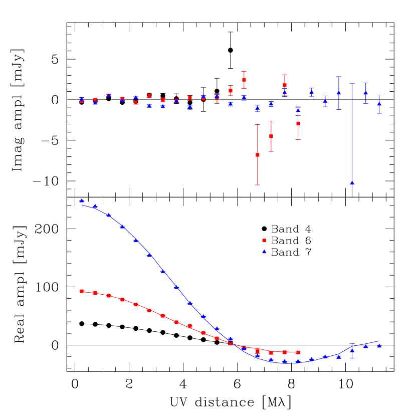
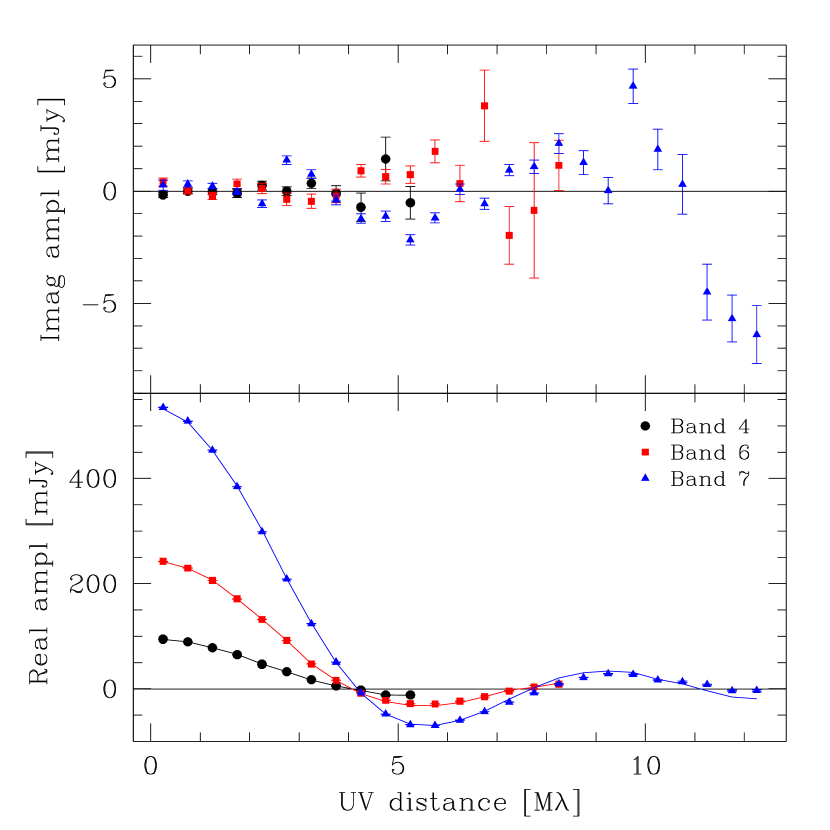
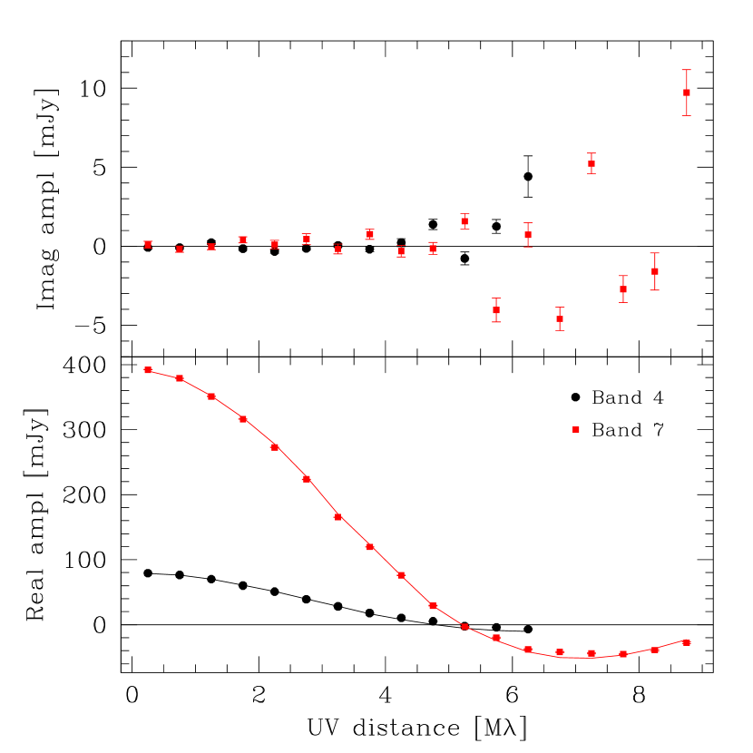
Although a uniform disc model provides good fits to all our observations, residual structure clearly remains. This is discussed in more detail in § 5.3. While in most cases this concerns small-scale structure, we found that for a number of spws, particularly those in Band 7 of the Mira observations, excess flux at short baselines affected the fits. This excess can be seen in the bottom right panel of Fig. 1 for baseline lengths below $\sim 2$ M$\lambda$. For the affected spws we restricted our fits to uv distances $>2$, or $>3$ M$\lambda$ for Band 4 and for Bands 6 and 7, respectively. The possible origin of the excess, particularly for Mira A, is discussed in § 5.4.

The measured sizes and flux densities are used to obtain the source brightness temperature using

$$T_{\rm b}={{1.97\cdot 10^{-8}\cdot S_{\nu}\cdot c^{2}}\over{\nu^{2}\cdot q\cdot\theta_{\rm maj}^{2}}}\leavevmode\nobreak\ {\rm K}.$$ (1)

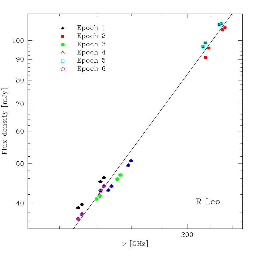
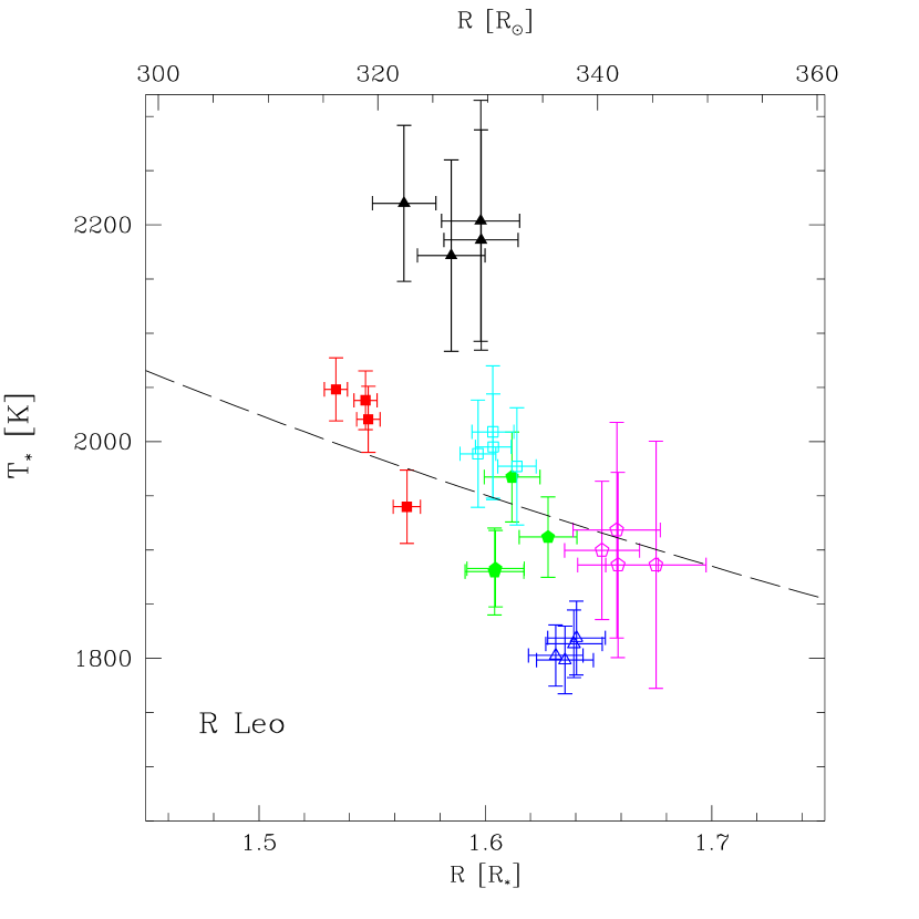
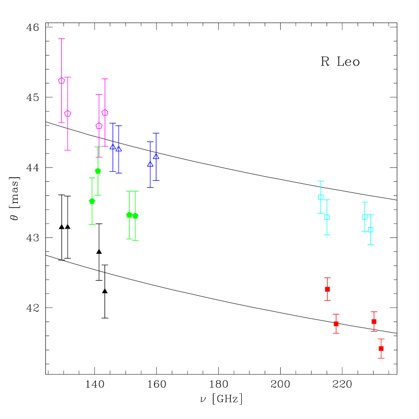
In this equation $S_{\nu}$ is the stellar flux density in mJy, $\theta_{\rm maj}$ the major axis in mas, $q$ the axis ratio ($\theta_{\rm min}/\theta_{\rm maj}$), $\nu$ the frequency in GHz, and $c$ the light-speed in m s^-1. The results for the flux density versus frequency, size versus frequency, and temperature versus size relations are shown in Figs  1, 2, 3, and 4. These figures also show the quality of the uv fits.

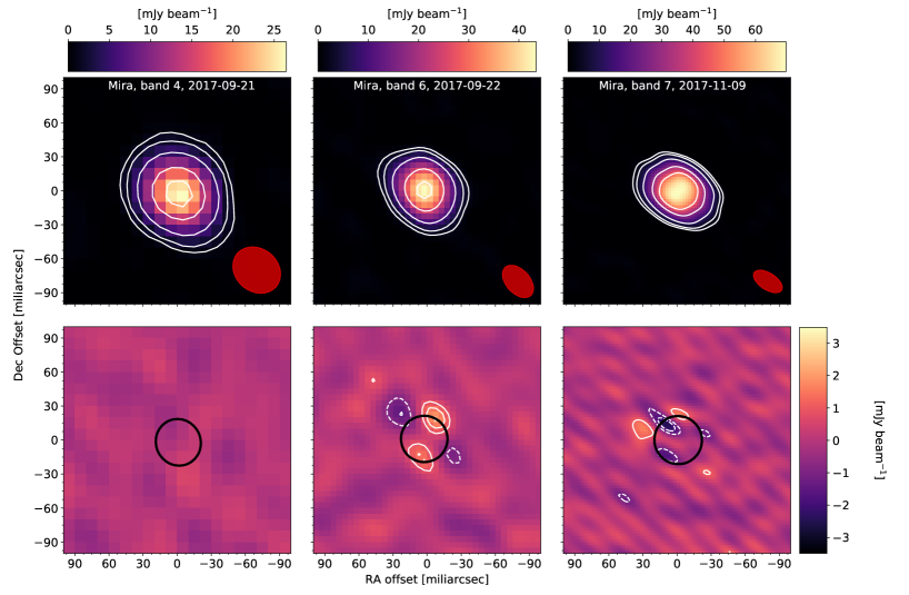
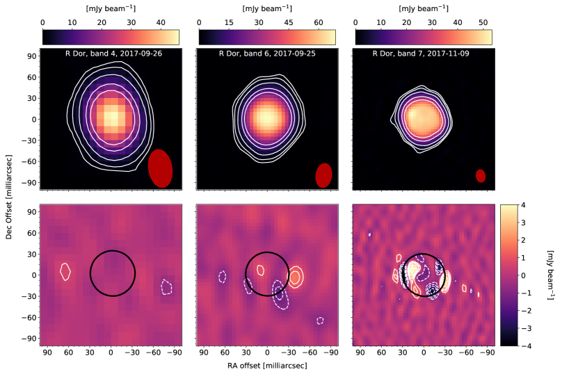
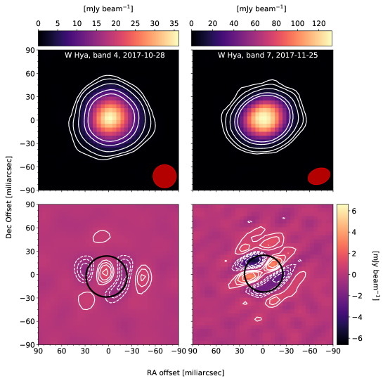
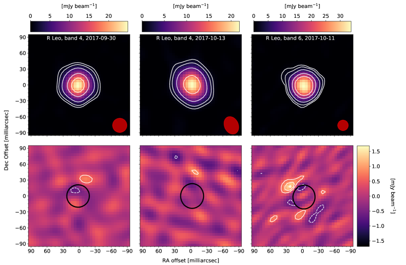
For illustration, we also produced images for all of the observations of Mira A, R Dor, and W Hya, as well as three of the epochs for R Leo. These are shown in Figs 5, 6, 7, and 8. The images were produced using uniform weighting in order to reach the highest resolution. Hence, the rms in the images is significantly higher than the rms reached when using Briggs weighting with a robust parameter of $+0.5$ (presented in Table 1). The figures also show the residuals after subtracting the best-fit stellar disc model from the data in each spw.

Figure 5: Top row: Uniformly weighted continuum maps of Mira A in the three observed bands. The images serve as an illustration since the analysis is performed on the visibilities by uv fitting. The images are produced for a single spw, using the highest frequency spw in each observing band. Contours are drawn at $4,8,20,50,$ and $80\sigma$, where $\sigma=0.28,0.50,$ and $0.58$ mJy beam^-1 from left to right. The beam sizes, from left to right, are $45\times 38$, $34\times 21$, and $29\times 15$ mas. Bottom row: Residual images after subtracting the best-fit uniform disc model presented in Table 3. The models are fitted for the spectral windows individually and the subsequent residual image is produced using all spectral windows. The beam sizes, from left to right, are $45\times 37$, $33\times 21$, and $27\times 13$ mas. Contours are drawn at $-15,-10,-7,-5,-3,3,5,7,10,$ and $15\sigma$, where $\sigma=0.21,0.27,$ and $0.37$ mJy beam^-1 from left to right. The black ellipse indicates the size of the best-fit uniform stellar disc model for the spw presented in the top panel.

Figure 6: As Fig.5 for R Dor. Here $\sigma=0.25,0.26,$ and $0.38$ mJy beam^-1 from left to right in the top panels, and $\sigma=0.17,0.26,$ and $0.28$ mJy beam^-1 from left to right in the bottom panels. The beam sizes are $55\times 33$, $34\times 22$, and $18\times 13$ mas on the top row and $52\times 32$, $34\times 22$, and $16\times 11$ mas on the bottom row.

Figure 7: As Fig.5 for the two observations of W Hya, with $\sigma=0.14,$ and $0.33$ mJy beam^-1 from left to right in the top panels and $\sigma=0.12,$ and $0.22$ mJy beam^-1 from left to right in the bottom panels. The beam sizes are $30\times 30$, and $29\times 20$ mas on the top row and $30\times 30$, and $27\times 17$ mas on the bottom row.

Figure 8: As Fig.5 for R Leo. Only three of the epochs are shown for illustration. The Band 6 epoch from 11 October was restored with a circular beam to highlight the northwest extension. In the top row, $\sigma=0.22,0.30,$ and $0.25$ mJy beam^-1 from left to right. In the bottom row, $\sigma=0.19,0.29,$ and $0.20$ mJy beam^-1 from left to right. The beam sizes are $27\times 27$, $34\times 26$, and $20\times 20$ mas on the top row, and $31\times 27$, $33\times 25$, and $20\times 20$ mas on the bottom row.

5 Discussion

5.1 Parameterised model atmospheres

We constructed a simple parameterised model atmosphere based on the radio-photosphere model of RM97 to derive rough estimates for the physical conditions in the extended atmospheres probed by our ALMA observations. Since the density profile in the AGB atmosphere is significantly affected by pulsations and convective motions, we adopt a basic power-law description for the molecular hydrogen number density $(n_{\rm H_{2}})$,

$$n_{\rm H_{2}}(r)=n_{\rm H_{2},0}\times\bigg{(}{{r}\over{R_{\rm*}}}\bigg{)}^{-\alpha}.$$ (2)

In this case $n_{\rm H_{2},0}$ is the number density (in $cm^{-3}$) at the stellar photosphere, $R_{*}$ is the photospheric radius, and $\alpha$ is the power-law index. For comparison, an atmosphere in hydrostatic equilibrium can, in the region of interest, be described with a power-law exponent $\alpha\approx 9$. In a dynamical atmosphere, the exact density versus radius relation becomes complex and depends strongly on pulsation cycle with regions displaying slopes steeper than in the hydrostatic case, while others are significantly more shallow (e.g. Höfner et al., 2003). When convective motions are included, the average power-law exponent can also reach $\alpha\approx 6$ (Freytag et al., 2017). Density profiles with $\alpha<6$ are also typically used to describe the molecular atmosphere (e.g. Wong et al., 2016; Khouri et al., 2016b). We adopt $\alpha=6$ for our reference model.

For the temperature profile we either use the grey atmosphere profile also adopted in RM97 written as

$$T^{4}(r)=T^{4}_{R_{*}}\times(1-\sqrt{1-R^{2}_{*}/r^{2}}),$$ (3)

or a power law given by

$$T(r)=T_{R_{*}}\times\bigg{(}{{r}\over{R_{\rm*}}}\bigg{)}^{-\beta}.$$ (4)

In this equation $T_{R_{*}}$ is the temperature (in K) at the photosphere and $\beta$ the power-law index. Finally, we also approximate the ionisation profile with a power law in temperature, i.e.,

$$X_{\rm i}=X_{\rm i,3000}\times\bigg{(}{{T}\over{3000}}\bigg{)}^{\gamma}.$$ (5)

In this equation $X_{\rm i}=n_{e}/n_{\rm H_{2}}$, where $n_{e}$ is the electron number density. We fix the ionisation at $T=3000$ K to be $X_{\rm i,3000}=7\times 10^{-6}$, which would correspond to single ionisation of K, Na, Ca, and Al when assuming solar abundance. For the specific stellar models presented later, the power-law index $\gamma=8$, which fits the range provided by the detailed model calculations from RM97. The exact adopted value of $R_{*}$ for our sources (as discussed in § 2) does not affect any of our conclusions, and for different stellar radii the surface values of density and temperature can be scaled accordingly.

With these parameters, we can calculate the frequency dependent optical depth throughout the extended atmosphere by taking into account the relevant opacity sources. As found in RM97, of the possible processes that contribute to the opacity, the electron-neutral free-free emission dominates in the relevant temperature and density regime for the radio and (sub)millimetre wavelengths. Hence we only considered this process. We did confirm that the electron-ion free-free emission contributes at least an order of magnitude less opacity even in the warmest, most ionised, and densest regions of our standard model. We only consider interactions of the electrons with purely atomic hydrogen in our calculations. This is in contrast to the study in RM97 in which an equilibrium state was assumed between atomic and molecular hydrogen. As was already noted in Bowen (1988) however, the formation rate of molecular hydrogen in the shocked atmosphere of an AGB star can be slow. The RM97 authors argued that for high densities ($>10^{12}$ cm^-3) in the extended atmosphere, the equilibrium time is $<250$ days. Since this is less than a typical pulsation period, RM97 assumed equilibrium conditions. However, for most of our sources, we find densities that are $<10^{12}$ cm^-3 throughout a large part of the atmosphere. Also, recent models and observations (e.g. Khouri et al., 2016a; Freytag et al., 2017) have shown that the timescales for significant changes due to convective motions and/or shocks can be measured in days or weeks. Hence we assume that equilibrium conditions are not reached. In case there is a significant molecular hydrogen component after all, the effective opacity decreases by up to a factor of five and our derived densities (or ionisation) would need to be increased. To calculate the opacity, we use the RM97 third-order polynomial fits to the absorption coefficients calculated by Dalgarno & Lane (1966). We note that another calculation and approximation is given in Harper et al. (2001), which is consistent within $\sim 10\%$ across the temperature range that we probe in the AGB atmosphere.

Table 4: Model atmosphere: fixed parameters

$n_{\rm H_{2},0}$	$4\times 10^{12}$ cm-3
$\alpha$	$6$
$T_{R_{*}}$	$2500$ K
$\beta$	grey atmosphere
$X_{\rm i,3000}$	$7\times 10^{-6}$
$\gamma$	$8$

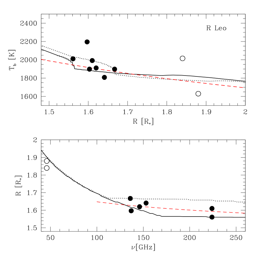
With the calculated opacities, we determine brightness temperature profiles using standard radiative transfer in the Rayleigh-Jeans limit. From these profiles we derive the frequency dependent stellar disc brightness temperature and size that can be directly compared with the observations. We assume a uniform stellar disc with a radius $R(\nu)$, which is the radius where the brightness temperature has dropped by $50\%$ in units of stellar radii $R_{*}$. The angular size, $\theta$, can be directly related to $R(\nu)$ by dividing it by the adopted angular stellar radius from Table 2. We focus in particular on the frequency-size and size-temperature relations as presented in Figs. 1, 2, 3, and 4 for the observations. As the opacity is proportional to the density (with exponent $2$) and ionisation (linearly), in addition to the inverse quadratic dependence on frequency, it is clear that there are degeneracies between the various parameters used to describe the extended atmosphere. Using the above exponents and the power-law components from Eqs $1-5$, we see that the optical depth $\tau_{ff}\propto r^{-(\gamma\beta+2\alpha)}\nu^{-2}$. Since the temperature is best constrained by the observations at different wavelengths, the ionisation and number density are most degenerate. Although the power-law approximation is likely far from reality, with shocks and pulsations producing density and temperature profiles that cannot be described using simple formulae, a number of conclusions can still be drawn from a small parameter study. A coupling of a dynamic and/or convective atmosphere code with the full continuum radiative transfer is beyond the scope of this paper.

Figure 9: Brightness temperature vs. size (left column) and size vs. frequency (right column) relations for model atmospheres (see text) with different power-law slopes for the density profile $(\alpha$, top), temperature profile ($\beta$, middle), and ionisation ($\gamma$, bottom). The two dashed lines indicate the range of the observed slopes of the size vs. frequency relation ($\eta$). Standard parameters are given in Table 4. We vary $\alpha$ from $5$ (blue) to $9$ (red) in steps of $0.5$. We vary $\beta$ from $0.3$ (blue) to $1.5$ (red) in steps of $0.2$ and include the grey atmosphere model (dark blue). We vary $\gamma$ from $2$ (blue) to $12$ (red) in steps of $1$.

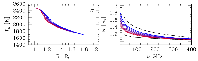
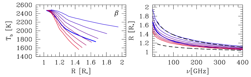
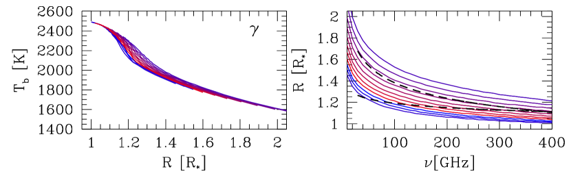
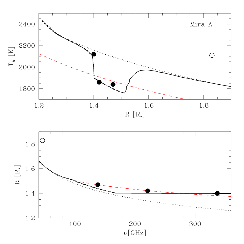
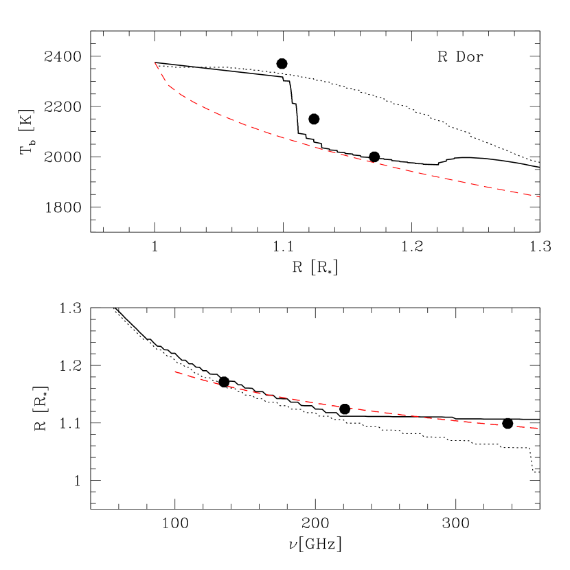
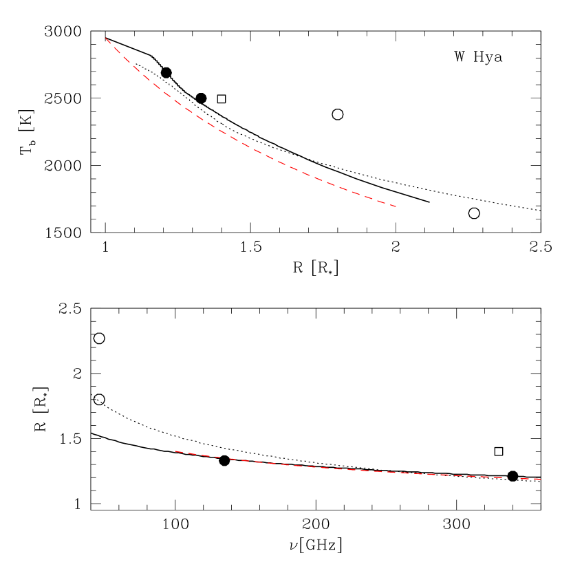
In Fig. 9, we show the size versus frequency and brightness temperature versus size relations for models with different $\alpha,\beta,$ and $\gamma$. The fixed model parameters for the plotted models are given in Table 4. In the figures we also indicate the observed range of slopes $(\eta)$ of the size versus frequency relation derived from the observations. From this is it clear that the lowest of the derived values of $\eta$ observed for Mira A, R Dor, and R Leo cannot be reproduced for any but the steepest density profiles ($\alpha>9$) and for none of the temperature or ionisation profiles. One of the most straightforward ways to match the shallow size versus frequency relations observed is to include a transition region with a sudden increase in opacity. Such a transition could naturally be related to a shock travelling through the extended atmosphere and mimics the density behaviour in dynamical atmopshere models (e.g. Bowen, 1988; Höfner et al., 2003) that have density variations up to a factor of $\sim 10$. We thus produce a model, which we describe as a “layer” model that has a ten times increase in $\tau_{\rm ff}$ at a single “shock” radius ($R_{s}$) to investigate if this could reproduce the observations. Including such an opacity increase specifically changes the stellar profile by introducing a region that is sufficiently optically thick so that there is no noticeable change of size with increasing frequency (within the observed frequency range). It can also produce limb brightening effects or ring-like structures in the residual maps once the layer has moved further out. As a result, the size determined using a uniform stellar disc increases, thereby producing a sharp drop in the temperature versus size relation and a leveling off of the size versus frequency relation. Ring-like structures related to this effect have possibly been seen around Betelguese (O’Gorman et al., 2017) and IRC+10216 (Matthews et al., 2018).

We discuss the modelling results for the four stars separately. We adopted the standard ionisation description for all stars. We note that we treat the different epochs presented in this paper for all stars except R Leo as sufficiently simultaneous in this analysis. The results are shown in Fig. 10.

Figure 10: Extended atmosphere models for Mira A (top left), R Dor (top right), W Hya (bottom left), and R Leo (bottom right) that can reproduce our observations. For each star the top panel shows the temperature vs. radius relation and the bottom panel shows the size vs. frequency relation. The solid circles are the measurements presented in this paper, and are taken as an average of all spws per observations. The open circles are 46 GHz radio observations (Matthews et al., 2015, 2018) shown for comparison. The radio observations were taken several years before the ALMA observations. In the panels for W Hya, the open square indicates the ALMA observations taken approximately 2 years earlier (Vlemmings et al., 2017). The thick solid lines are the models described in the text. In the top panels for each star, the red dashed line represents the assumed temperature profile. In the bottom panels for each star, the red dashed lines represent the size vs. frequency power-law relation fitted to the observations. For Mira A and R Dor, the dotted line represents a model without a high-opacity layer. For W Hya the dotted line represents the grey atmosphere model with $n_{H_{2}}\propto r^{-3}$ that comes closest to describing the radio observations. For R Leo the dotted line represents the model for which the layer location has shifted (see text).

5.1.1 Mira A

The slope of the size versus frequency relation for Mira A is shallow, where $\eta=-0.087\pm 0.006$ is determined from the Band 4 and 6 observations, and $\eta=-0.053\pm 0.002$ between the Band 7 observations taken $\sim 1.5$ month later and the Band 4 observations. The observations can be reproduced by a typical density profile with $n_{H_{2},0}=1\times 10^{13}$ cm^-3 and $\alpha=6$. For the temperature, a grey atmosphere with $T_{R_{*}}=2800$ K is consistent with the measured brightness temperatures. Additionally, the low $\eta$ and apparent abrupt drop of $T_{b}$ between the Band 6 and 7 observations requires a sudden increase (moving inwards) in opacity by at least a factor of 10 at $R_{s}=1.4\leavevmode\nobreak\ R_{*}$ in our model framework. We do not cover a sufficient range of radii to determine the thickness of the region with elevated opacity. Considering the relation between opacity and the modelling parameters, the opacity change can be produced by an increase of the density by at least a factor of three or a change of ionisation by a factor of $10$ or a combination of these. A significant change in temperature would have affected the brightness temperature versus size relation. To indicate how our model compares with radio-wavelength observations at 46 GHz (Matthews et al., 2015), we also present the average of the major and minor axis of these observations in the figure even though the radio epoch was three years before the ALMA observations. We find that our model underestimates the brightness temperature measured at 46 GHz by almost $20\%$ while it underestimates the radius by $10\%$. Considering that the temperature uncertainty of the radio observations is $\sim 20\%$ and the ellipticity is almost $18\%$, the model could be consistent. The size measurements of the previous ALMA observations at 96 and 230 GHz are also consistent but the derived brightness temperatures are $>20\%$ higher (Vlemmings et al., 2015; Matthews et al., 2015).

The layer of enhanced opacity we derive for Mira A is likely related to shocks originating from stellar pulsations and/or convection. Since we do not have sufficient observing epochs spread over a few weeks timescale taken at similar frequencies, we are unable to determine a motion of the layer. Alternatively, it might not be an actual spherical layer, as we observe asymmetries such as a mild elliptical shape and compact structures in our residual maps. Our models are not yet able to determine the effect of such structures. The derived density and temperature relations should thus be seen as rough indications only. Still, deviations from the densities we find by a factor of three or more would, in our framework, produce significantly different stellar sizes and are thus unlikely unless compensated by differences in ionisation or another opacity source.

5.1.2 R Dor

The sizes of R Dor observed at the different frequencies are, in stellar radii, the smallest of our sample. Similar to Mira A, the change of size with frequency is low ($\eta=-0.078\pm 0.001$ between Band 4 and Band 6, and $\eta=-0.059\pm 0.013$ in Band 7). A combination of a fast drop in temperature and the low $\eta$ also implies the existence of a layer with increased opacity around R Dor. Since the measured size is small, we can reproduce the profiles with a lower density of $n_{H_{2},0}=4\times 10^{12}$ cm^-3 and $\alpha=6$. The temperature is well reproduced by a grey atmosphere with $T_{R_{*}}=2375$ K. The opacity enhancement (by a factor of $10$) around R Dor occurs at $R_{s}=1.11\leavevmode\nobreak\ R_{*}$. For R Dor, the ellipticity increases markedly towards the higher frequencies in Band 7 and also several clear residual emissions occur both towards the star and in the limbs. Although the similar caveats should be considered as for Mira A, the observations imply that the layer is related to the asymmetric structures that are likely (convective) shocks. Alternatively or additionally, the increased opacity so close to the photosphere could arise owing to the presence of a higher ionisation region related to a possible chromosphere. No long wavelength observations of R Dor exist for comparison because of its low declination.

5.1.3 W Hya

W Hya is the only star in our sample that displays a slope $\eta$ that can be reproduced without adding a region with enhanced opacity ($\eta=-0.160\pm 0.007$ in Band 4, and $\eta=-0.104\pm 0.003$ in Band 7). For this, we need a density profile with $n_{H_{2},0}=4.5\times 10^{12}$ cm^-3 and $\alpha=6$. A temperature profile with $T_{R_{*}}=2950$ K and $\beta=0.8$ produces a slightly better correspondence with the data than a grey body atmosphere model. However, a grey body atmosphere with $n_{H_{2},0}=3\times 10^{12}$ cm^-3 and $\alpha=3$ is better able to reproduce the radio observations as was already noted for W Hya by RM97. This likely reflects the complex nature of the AGB extended atmosphere where a simple single power law is not sufficient to characterise the density and temperature. W Hya also shows significant residuals from a simple stellar disc model, both in the observations presented in this work and the previous ALMA observations (Vlemmings et al., 2017).

5.1.4 R Leo

R Leo presents a complex case. As we discuss in § 5.2, a clear expansion is seen. This points to an outward motion of a shock wave. When adjusting each epoch for the fitted outward motion of $V\approx 11$ km s^-1 and fitting a single power law to the adjusted size versus frequency relation, we find $\eta=-0.042\pm 0.015$. We can reproduce the range of observed sizes and temperatures by introducing an increased opacity layer as shown in Fig. 10. The layer moves from $1.57\leavevmode\nobreak\ R_{*}$ to $1.66\leavevmode\nobreak\ R_{*}$ and the underlying density profile has $n_{H_{2},0}=1\times 10^{13}$ cm^-3 and $\alpha=5.0$. The temperature is described by a grey atmosphere model with $T_{R_{*}}=2800$ K. Since it appears that at least part of the expansion of R Leo is asymmetric, with significant residuals from a uniform stellar disc towards the north-east, the apparent layer might in reality be a directional shock wave propagating through the extended atmosphere.

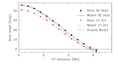
5.2 Expansion of R Leo

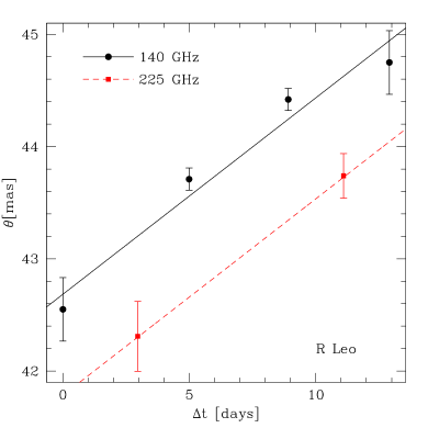
ALMA observed R Leo within two weeks on four and two occasions in Band 4 and Band 6, respectively, at fairly similar frequencies in each given band. We are thus able to investigate its time variable behaviour in detail. Looking at the flux density variations, we find differences of on average $5\%$. These can mostly be attributed to absolute flux calibration uncertainties, even though the same flux calibrator was used. However, we also note a clear trend of increasing radius and ellipticity with time. In Fig. 11 we show a comparison of the uv data and model fits for the first and last observing epoch in Band 4. The fit indicates that the size change is robustly determined. In Fig. 12 we display the measured size against the time after the first observations for both Band 4 and Band 6. In this plot we adjust all measurements to 140 and 225 GHz for the Band 4 and Band 6 data, respectively, using the individually fitted slopes to the frequency-size relations. We can fit a linear expansion of $0.17\pm 0.02$ mas day^-1 to the Band 4 data and find that this is consistent with the size measurements during the two epochs at 225 GHz. These measurements imply that the continuum surface seen in the millimetre wavelength observations is expanding at $10.6\pm 1.4$ km s^-1 when assuming a distance to R Leo of 71 pc. The fact that the 140 and 225 GHz surfaces undergo a similar expansion implies a bulk motion of material that encompasses almost $0.2\leavevmode\nobreak\ R_{*}$. A motion of the continuum surface can occur because of changes in density, ionisation and/or temperature. The temperature in the region that we are probing does not seem to change by more than $\pm 5\%$ (most likely due to absolute flux calibration uncertainties). Such a variation would produce a change in ionisation of $\sim 50\%$ and a similar change in opacity. According to our models for R Leo, this would result in a change of measured radius, at 140 GHz, of $\sim 0.05\leavevmode\nobreak\ R_{*}$. This assumes the temperature changes throughout the entire envelope which requires radiative heating, which is unlikely. The radius change would be significantly less if the temperature change is only local. Hence, the motion that we are seeing is likely due to density or ionisation changes (by factors $>2$ or $>4$, respectively).

The measured velocity matches the velocity dispersion seen in the gravitationally bound molecular gas around a number of stars (e.g. Hinkle et al., 1997; Wong et al., 2016; Vlemmings et al., 2017, 2018). Since the star also increases its ellipticity, the motion is not spherically symmetric. The expansion velocity taking the major axis values alone would correspond to $12\pm 1$ km s^-1 and that of the minor axis to $9\pm 1$ km s^-1. Note that if the movement occurs mostly in only one direction and not equally in opposite directions (which is unlikely if it is a result of convective motions), the inferred velocities are up to a factor of two higher. In any case, the velocity is less than the escape velocity, which is $\sim 34$ km s^-1 at $1.6\leavevmode\nobreak\ R_{*}$ for a star with $M=1$ M_⊙. The velocity exceeds the local sound speed in the atmosphere, which is $\sim 5$ km s^-1. It is also larger than the velocities of $\lesssim 8$ km s^-1 found at $R\sim 1.6\leavevmode\nobreak\ R_{*}$ in current convection models (Freytag et al., 2017).

Figure 11: Comparison of the real part of the uv visibilities between R Leo Band 4 observations taken on 2017-09-30 (black solid line and circles) and 2017-10-13 (red dashed line and squares). In most cases the error bars are less than the symbol size. The lines represent the uniform disc model, where the long-dashed blue line corresponds to the best-fit model of the 2017-10-13 observations scaled to the flux density of the 2017-09-30 observations. Although the difference in flux density is most likely predominantly caused by the uncertainty in absolute flux calibration, the long-dashed blue line shows that the change in radius of the model is robustly determined.

Figure 12: Average diameter $\theta$ vs. observing time after the first epoch (2017-09-30) for the star R Leo. The black circles indicate the radius at 140 GHz in Band 4 and the red squares are the fitted radii at 225 GHz in Band 6. The black solid line is the error weighted fitted expansion of the optically thick surface. The expansion velocity corresponds to $10.6\pm 1.4$ km s^-1 (assuming a distance of $71$ pc). The red dashed line is the fit to the $140$ GHz radii shifted by a time lag of $-5$ days.

5.3 Asymmetries and hotspots

Previous observations of AGB stars at radio and sub-mm/mm wavelengths have revealed a variety of asymmetries and hotspots in the extended atmospheres. Radio observations at different epochs have shown significant ellipticity, brightness asymmetries and non-uniform surfaces (e.g. RM97 Reid & Menten, 2007; Matthews et al., 2018). ALMA observations of Mira A and W Hya also revealed a mottled surface structure at sub-mm/mm wavelengths (Vlemmings et al., 2015; Matthews et al., 2015; Vlemmings et al., 2017). The most prominent of these was the detection of a hotspot with $T_{\rm b}>50000$ K on the surface of W Hya. As can be seen in the residuals from a uniform stellar disc model and the uv model fits for the sources presented in this work (Figs 5, 6, 7, and 8), all stars display asymmetries and/or hotspots to various degree. In some cases, negative residuals are seen that are similar in strength to the positive features. This is a natural result when determining the residuals after subtracting a best-fit uniform-disc model, which minimises the intergrated flux across the disc.

Mira A: Our observations of Mira A indicate that, at the current epoch, the star is relatively circular with a marginally significant ellipticity of a few percent seen in the Band 6 data. This is in contrast with previous ALMA observations that indicate an ellipticity between $10-20\%$ (Vlemmings et al., 2015; Matthews et al., 2015). While the previous observations had significant residuals that could indicate a strong hotspot, the current data only have a weak spotted structure, predominantly in the limb of the disc. This could be related to a (non-uniform) enhanced opacity layer, such as included in the atmosphere models, with changes in density or ionisation by a factor of $\sim 3$ or $\sim 10$, respectively.

R Dor: R Dor shows strong residual hotspots, especially in the Band 7 observations. At those frequencies we can determine a lower limit to $T_{\rm b}$ for both brightest hotspot of $>3300$ K above the average stellar disc temperature. The actual temperature could be significantly higher if the hotspot sizes are smaller than the formal limit of $<6\times 3$ mas obtained from a fit to the residual image and uv data. The brightness variation across the stellar surface appears to correlate with structure seen at visible wavelengths (Khouri, 2018, and in prep.). In a comparison between the Band 6 and 7 observations, there also appears to be a correspondence between the structure seen at both wavelengths. The two frequencies probe a slightly different region of $\sim 0.03$ R_∗ in depth. If the structures are indeed the same, they would thus have a vertical extent of at least $8\times 10^{11}$ cm ($\sim 0.05$ au). Since R Dor appears to be the star with the smallest (sub)millimetre size compared to its stellar radius as determined from infrared observations, we are potentially probing very close to a chromosphere if it is present. Notably, the ellipticity of R Dor increases towards the shorter wavelengths in Band 7, with an ellipticity up to $\sim 6\pm 1\%$ at a position angle of $44\pm 2^{\circ}$. There is no correspondence between this position angle and the apparent rotation axis (Vlemmings et al., 2018).

W Hya: As was found previously (Vlemmings et al., 2017), W Hya shows strong deviations from a uniform disc. Hotspots and negative patches are seen in both the Bands 4 and 7 observations. As discussed above, in the event of strong hotspots, negative bowls also naturally occur when a uniform disc with spots is fitted by a disc alone. Negative patches towards the star can also occur owing to an increase of opacity along the line of sight. In the limb these patches can be the result of a convolution of the beam with the residuals that remain when a top-hat stellar disc is subtracted from a more shallow stellar profile. In the Band 4 observations, we find that the prominent hotspot can be constrained to $<5.3\times 5.3$ mas, which implies $T_{\rm b}>3750$ K. In Band 7, the two spots are very compact ($<2.6\times 2.6$ mas) with $T_{\rm b}>10000$ K. This is consistent with the previously observed hotspot. We find no correspondence in the positions of the spots seen in Bands 4 and 7, nor with the position of the spot seen in previous observations. Since the region probed at the shorter wavelengths (at $\sim 1.2\leavevmode\nobreak\ R_{*}$) is still optically thick at longer wavelengths (where we find a radius of $\sim 1.33\leavevmode\nobreak\ R_{*}$), the Band 7 spots are likely obscured at Band 4. Additionally, the current observations were taken almost a month apart, while the previous observations were taken two years earlier. Since significant changes in the optical are seen on timescales of weeks (Khouri et al., in prep.) and convective motions and associated shocks operate on similar timescales. it is likely that the lifetime of the hotspots is of the same order.

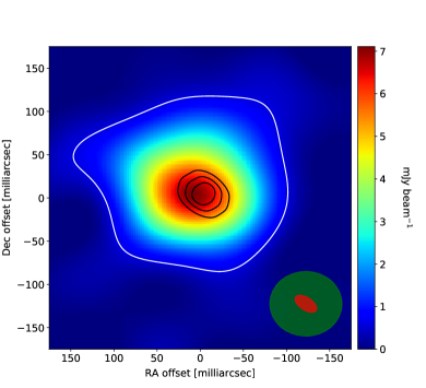
R Leo: Although the multi-epoch observations of R Leo show a clear signature of an expanding layer, there is no sign of strong hotspots. We only see an extension in the north-east in the Band 6 observations. This structure appears marginally resolved ($\sim 10\times 5$ mas implying $T_{\rm b}\sim 1000$ K) along the limb of the star, which means it could be related to the layer invoked to explain the observed sizes and temperatures. The ellipticity also increases from nearly circular to $\sim 7\%$ ellipticity with a position angle due north. The fact that the residuals remain towards the north-east implies that the true shape of the stellar disc is not quite elliptical and that an expansion of material with a size of up to an entire quarter of the stellar disc is occurring. Such a large size would not be inconsistent with that of a large convective cell.

5.4 Extended emission surrounding Mira A

Figure 13: Residual map of the extended emission around Mira A at 332 GHz. We have subtracted the best-fit uniform disc model after fitting to the data with uv distance $>3$ M$\lambda$. The residual image is made using Briggs weighting and restricting the baselines to $<2$ M$\lambda$, which results in a synthesised beam of $84\times 75$ mas at a position angle of $89.6^{\circ}$ (indicated in green in the bottom right corner). The black contours are the corresponding map of Mira A using all data drawn at $0.2,0.5,$ and $0.8$ times the peak intensity. The beam size for all data is shown in red in the bottom right corner. The white contour is drawn at $\sim 20\sigma$, with $\sigma=0.13$ mJy beam^-1. The residual emission has a peak of $7$ mJy beam^-1, which corresponds to $\sim 3\%$ of the stellar flux density.

As noted previously, in particular the shortest wavelength Mira data show a clear deviation from a simple stellar disc model at the largest angular scales. We show this residual, for one of the spws, in Fig. 13. The same emission is seen in all spws and has an almost linear increase of integrated flux density from $12$ mJy at $330$ GHz to $31$ mJy at $344$ GHz. It is immediately apparent that the extended emission peaks towards the east of the star and extends over almost $5\leavevmode\nobreak\ R_{*}$. The extent and morphology bears resemblance to the emission seen in SO, CO, and TiO₂ lines shown in Khouri et al. (2018) and extends out to the dust ridges seen with SPHERE/ZIMPOL in the same paper.

We suggest three possible origins of the extended emission. If the emission originates from circumstellar dust emission close to the star it would represent a dust mass of $\sim 2\times 10^{-7}$ M_⊙ at $T=1000$ K adopting circumstellar dust properties from Knapp et al. (1993). The large flux density difference between the spws would argue against the emission being due to dust. However, since the emission only corresponds to a few percent of the subtracted stellar emission, the flux density measurements might be uncertain. If the emission is due to dust, it is however unclear why the VLT/SPHERE observations (Khouri et al., 2018) show such a clear lack of dust scattering emission in the region.

A second possibility would be that the emission is due to many weak residual spectral lines remaining in the data. Although a significant effort was made to remove the obvious lines, the line density at the shortest wavelengths around Mira A is significant. If we are seeing stacked lines this could explain the correspondence with the aforementioned stronger lines arising in the same region. It would hint at an asymmetric mass-loss process that is not surprising considering the complexity of the Mira system. It is not clear why the flux density of the emission changes almost linearly with frequency.

Finally, the emission could represent the electron-neutral free-free emission from the optically thin extended atmosphere. Although we find that the brightness profile is generally well represented by a stellar disc model, the true profile could have weaker emission extending out to several stellar radii. The Mira 46 GHz observations indicate an extent of almost $4\leavevmode\nobreak\ R_{*}$. Furthermore, although we were unable to produce a similar high fidelity map at Band 6, at those frequencies a short-baseline excess was also found. This hypothesis does not naturally explain the strong flux density increase with frequency, but potentially rapid changes of opacity could be involved. If this is indeed the cause for the emission, it would also indicate quite a non-symmetric envelope.

At the moment we cannot rule out any of the possible origins with certainty, although dust emission appears unlikely. To distinguish between these possibilities, sensitive observations at high frequencies and improved models are needed.

6 Conclusions

We have shown that multi-epoch and multi-frequency high angular-resolution observations with ALMA can be used to probe the extended atmospheres of AGB stars. This has allowed us to constrain the density, ionisation, and temperature between $\sim 1-2\leavevmode\nobreak\ R_{*}$. The main source of uncertainty on the temperature determination has been shown to be the absolute flux calibration accuracy of ALMA. Specifically, multi-epoch observations of the same flux- and gain-calibrator pair over four epochs of ALMA Band 4 observations indicate that an uncertainty of $\sim 5\%$ can only be reached with sufficient observations within a short timescale. For single epoch observations, the uncertainty, even at low frequency, is closer to $10\%$. Still, size measurements and surface maps can be made with great accuracy.

We find that parameterised atmosphere models can describe the observations for typical surface hydrogen number densities between $n_{\rm H_{2},0}=3\times 10^{12}-1\times 10^{13}$ cm^-3 and photospheric temperatures of $T=2300-3000$ K. These models assume the electron-neutral free-free process as the dominant opacity source as previously found in RM97. However, for R Dor, Mira A, and R Leo a layer of increased continuum opacity is needed to reproduce the shallow slope of the size versus frequency relation. This layer, of unknown thickness, could be due to a sudden increase of neutral hydrogen density or effective ionisation or a combination of this. Alternatively an unknown additional opacity source is needed. It is likely that the layer is non-uniform and it might be related to convective shocks.

A mottled structure of spots can be seen most clearly on the surface of R Dor and W Hya. The brightness temperature of the brightest spot of R Dor is $>3000$ K while the two brightest spots on the surface of W Hya have $T_{\rm b}>10000$ K, which is consistent with previous observations (Vlemmings et al., 2017). The spots likely represent the shocks that cause the formation of a low-filling factor chromosphere. The timescale of these spots is of the order of a few weeks at most.

Our six epochs of observations of R Leo show a linear increase in measured size with an expansion velocity of $10.6\pm 1.4$ km s^-1. We suggest that the expansion is related to the motion of the aforementioned high opacity layer. The velocity is consistent with the typical line widths seen in the stellar atmosphere but does not exceed the escape velocity.

In particular for Mira A, we find significant excess flux at the shortest baseline lengths compared to a uniform stellar disc model. The most likely explanation is that we are seeing either an asymmetric distribution of optically thin neutral-ion free-free emission out to almost $3$ R_∗, or the effect of stacking weak emission lines in what were thought to be line-free regions of the spectrum. However, although unlikely, we cannot yet fully rule out that the emission comes from warm circumstellar dust.