The evolving X-ray spectrum of active galactic nuclei: evidence for an increasing reflection fraction with redshift

Abstract

The cosmic X-ray background (XRB) spectrum and active galaxy number counts encode essential information about the spectral evolution of active galactic nuclei (AGNs) and have been successfully modeled by XRB synthesis models for many years. Recent measurements of the $8$–$24$ keV AGN number counts by NuSTAR and Swift-BAT are unable to be simultaneously described by existing XRB synthesis models, indicating a fundamental breakdown in our understanding of AGN evolution. Here we show that the $8$–$24$ keV AGN number counts can be successfully modeled with an XRB synthesis model in which the reflection strength ($R$) in the spectral model increases with redshift. We show that an increase in reflection strength with redshift is a natural outcome of (1) connecting $R$ to the incidence of high column density gas around AGNs, and (2) the growth in the AGN obscured fraction to higher redshifts. In addition to the redshift evolution of $R$, we also find tentative evidence that an increasing Compton-thick fraction with $z$ is necessary to describe the $8$–$24$ keV AGN number counts determined by NuSTAR. These results show that, in contrast to the traditional orientation-based AGN unification model, the nature and covering factor of the absorbing gas and dust around AGNs evolve over time and must be connected to physical processes in the AGN environment. Future XRB synthesis models must allow for the redshift evolution of AGN spectral parameters. This approach may reveal fundamental connections between AGNs and their host galaxies.

1 Introduction

At rest frame energies above 2 keV, the X-ray spectral energy distribution (SED) of unabsorbed active galactic nuclei (AGNs) can be described as the sum of just two interconnected components. The first of these is a cutoff power-law spectrum with photon index $\Gamma$ and cutoff energy $E_{\mathrm{cut}}$ that is consistent with being produced by the Compton up-scattering of ultraviolet (UV) photons from the accretion disc in a hot tenuous corona (e.g., Galeev, Rosner & Vaiana, 1979; Haardt & Maraschi, 1991, 1993; Haardt, Maraschi & Ghisellini, 1994). The rapid variability of the power-law, as well as novel micro-lensing size measurements, both indicate that the corona is compact and located close to the central supermassive black hole (SMBH; e.g., Reis & Miller 2013; Zoghbi et al. 2013; MacLeod et al. 2015; Kara et al. 2016). The second component of an AGN spectrum is one or more reflection spectra produced by the interaction of the power-law with cold dense gas situated out of the line-of-sight (e.g., George & Fabian, 1991; Matt, Perola & Piro, 1991; Ross & Fabian, 1993; Ross, Fabian & Young, 1999; Ross & Fabian, 2005; García & Kallman, 2010). At energies above 2 keV, the reflection spectrum adds an Fe K$\alpha$ line at $6$–$7$ keV and a Compton ‘hump’ between $\approx 20$–$40$ keV to the intrinsic power-law. Deep exposures of bright nearby AGNs find a low-contrast, relativistically broadened Fe K$\alpha$ line along with a strong and narrow line ‘core’ at 6.4 keV indicating that both the inner accretion disc and distant optically thick gas in the AGN environment contribute to the reflection signal (e.g., Nandra et al., 2007; de la Calle Pérez et al., 2010; Bhayani & Nandra, 2011; Patrick et al., 2012; Walton et al., 2013; Mantovani, Nandra & Ponti, 2016). Typically only the narrow Fe K$\alpha$ line is measurable in fainter AGNs outside the local Universe (e.g., Mainieri et al., 2007; Marchesi et al., 2016).

Efficient X-ray reflection only occurs in relatively cold Compton-thick (or near Compton-thick) gas (e.g., George & Fabian, 1991; Matt et al., 1991). Since even unobscured AGNs exhibit this distant reflection signature, the gas must lie out of the line-of-sight, but still subtend a significant solid-angle as seen from the X-ray source. Identifying the origin of the distant reflector has been a significant observational challenge as, until recently, the narrow Fe K$\alpha$ line was the only direct probe of this spectrum. Nevertheless, measurements of the Fe K$\alpha$ line width from Chandra observations indicated that the reflector is likely connected to the obscuring gas associated with AGN unification models (e.g., Nandra, 2006; Shu, Yaqoob & Wang, 2010, 2011), and the equivalent width of the Fe K$\alpha$ line appears to decrease with AGN luminosity (an ‘X-ray Baldwin Effect’; e.g., Iwasawa & Taniguchi 1993; Shu et al. 2012; Ricci et al. 2013, 2014; Marchesi et al. 2016) similar to the observed decrease in the fraction of obscured, or Type 2, AGNs ($f_{2}$) with luminosity (e.g., Hasinger, 2008; Burlon et al., 2011; Merloni et al., 2014; Georgakakis et al., 2017). Therefore, the distant reflector appears to probe the high column density regions of the obscuring gas around AGNs. Since directly detecting AGNs that are absorbed by Compton-thick gas is extremely challenging at all wavelengths (Hickox & Alexander, 2018), the distant reflector can be used as a direct probe of the Compton-thick gas in the AGN environment. Crucially, if reflection signatures can be measured in AGNs at higher redshifts, then they could be used to probe the evolution of Compton-thick gas over time, which will be important for models of AGN fueling and feedback (e.g., Hopkins et al., 2006).

The strength of the distant reflector is also important for fitting the shape of the cosmic X-ray background (XRB). XRB synthesis models rely on a model AGN SED that is then integrated over luminosity and redshift (e.g., Comastri et al., 1995; Treister & Urry, 2005; Ballantyne, Everett & Murray, 2006; Gilli, Comastri & Hasinger, 2007; Draper & Ballantyne, 2009; Treister, Urry & Virani, 2009; Ballantyne et al., 2011; Ueda et al., 2014). It was established early on (e.g., Ueda et al., 2003) that a significant reflection strength (denoted by $R$) is needed to account for the observed peak of the XRB at $\approx 30$ keV. As the XRB itself is a poor constraint on $R$ (Akylas et al., 2012), different XRB models employ different assumptions on the value of $R$, but most assumed a constant $R\sim 1$, a value based on observations of bright, nearby AGNs (e.g., Ricci et al., 2017) and corresponds to an isotropic source above an infinite disk. Some models included the decrease of $R$ with luminosity (e.g., Gilli et al., 2007; Draper & Ballantyne, 2009), but all assumed that there was no redshift dependence. Despite the simplicity of the assumptions on $R$, the XRB models could successfully account for the XRB spectrum and much of the $\la 10$ keV data (e.g., Ballantyne et al., 2011). However, a hint that these models were incomplete was noted by Ajello et al. (2012) who found that none of the available XRB models could describe the Swift-BAT $15$–$55$ keV AGN number counts.

The broad ($3$–$79$ keV) bandpass and focusing optics provided by NuSTAR (Harrison et al., 2013) now allow the full AGN reflection spectrum (i.e., Fe K$\alpha$ line and Compton hump) to be analyzed for AGNs far beyond the local Universe. Most of the high-$z$ AGNs detected by NuSTAR in deep extragalactic survey fields (Civano et al., 2015; Mullaney et al., 2015; Lansbury et al., 2017) are still too faint to perform spectral fitting, but Zappacosta et al. (2018) was able to estimate $R$ from 63 of the brightest sources with a median $z=0.58$ and found a significant decrease of $R$ with X-ray luminosity. Similar results were also found by Del Moro et al. (2017) who analyzed stacked NuSTAR spectra from the deep fields. In addition, both studies found that the typical values of $R$ were $\la 1$. Unfortunately, neither group was able to disentangle redshift effects from the flux limited samples provided by the survey fields. These results are in striking contrast with the integrated results from the NuSTAR surveys. When both the $8$–$24$ keV luminosity function and numbers counts are computed from the NuSTAR data, large ($R\sim 2$) values of the reflection strength are needed in the XRB models to fit these data (Aird et al., 2015; Harrison et al., 2016). Even more interesting is the fact that, as was anticipated by Ajello et al. (2012), these high $R$ models cannot simultaneously fit both the NuSTAR and Swift-BAT number counts (Harrison et al., 2016). This problem was recently discussed by Akylas & Georgantopoulos (2019) who confirmed the fundamental shape difference in the survey data produced by the two missions, but were unable to identify any plausible systematic statistical or instrumental mechanism for the disagreement. As the Swift-BAT counts are predominantly from AGNs at $z<0.1$, and the median redshift of the NuSTAR catalog is $z=0.76$ (Harrison et al., 2016), the inability for models to explain both data sets may be indicating the presence of redshift evolution in the average AGN spectrum. Since the $8$–$24$ keV band probed by NuSTAR and Swift-BAT is sensitive to the Compton hump in the reflection spectrum, an evolving $R$ is a prime candidate to explain the discrepancy, and would indicate an increase in Compton-thick gas in the AGN environment at higher redshifts.

This paper presents a new X-ray background synthesis model that can evolve the average spectral parameters of AGNs in both luminosity and redshift with an initial focus of developing a model that can explain the discrepancy between the $8$–$24$ keV NuSTAR and Swift-BAT number counts. The next section describes the details of the model and its underlying assumptions, and we begin our analysis in Sect. 3 by presenting the $8$–$24$ keV number counts problem and considering various solutions. Based on the results of this preliminary work, Sect. 4 describes an XRB model with a physically-motivated evolving $R$ and compares it to the $8$–$24$ keV NuSTAR and Swift-BAT number counts. The results are discussed in Sect. 5 and conclusions are presented in Sect. 6. The paper assumes a standard flat $\Lambda$CDM cosmology: $H_{0}=70$ km s^-1 Mpc^-1, $\Omega_{m}=0.3$, and $\Omega_{\Lambda}=0.7$.

2 Description of the X-ray Background Synthesis Model

An XRB synthesis model consists of computing both the spectrum of the XRB as a function of energy ($E$, in keV),

$$\begin{split}I(E)=\frac{c}{H_{0}}&\int_{z_{\min}}^{z_{\max}}\int_{\log L_{\mathrm{X}}^{\min}}^{\log L_{\mathrm{X}}^{\max}}\frac{d\Phi(L_{\mathrm{X}},z)}{d\log L_{\mathrm{X}}}\\ &\times\frac{S_{E}(L_{\mathrm{X}},z)d_{l}^{2}}{(1+z)^{2}(\Omega_{m}(1+z)^{3}+\Omega_{\Lambda})^{1/2}}d\log L_{\mathrm{X}}dz,\end{split}$$ (1)

and the differential AGN number counts as a function of flux ($S$, defined over some energy band),

$$\begin{split}\frac{dN}{dS}(S)=\frac{K_{\operatorname{str}}^{\deg}c}{\ln 10H_{0}}&\int_{z_{\min}}^{z_{\max}}\frac{d\Phi(L_{\mathrm{X}},z)}{d\log L_{\mathrm{X}}}\\ &\times\frac{d_{l}^{2}}{(1+z)^{2}(\Omega_{m}(1+z)^{3}+\Omega_{\Lambda})^{1/2}}\frac{dz}{S}.\end{split}$$ (2)

In these two equations $d\Phi(L_{\mathrm{X}},z)/d\log L_{\mathrm{X}}$ denotes the hard X-ray luminosity function (HXLF), $S_{E}(L_{\mathrm{X}},z)$ is an average absorbed AGN X-ray spectrum with an unabsorbed $2$–$10$ keV luminosity $L_{\mathrm{X}}$ at redshift $z$, $d_{l}$ is the luminosity distance to $z$, and $K_{\operatorname{str}}^{\deg}=3\times 10^{4}$ converts the number counts from $\operatorname{str}^{-1}$ to $\deg^{-2}$. The integrals are evaluated from $z_{\min}=0$ to $z_{\max}=6$ and $\log(L_{\mathrm{X}}^{\min}/\mathrm{erg\ s^{-1}})=41.5$ to $\log(L_{\mathrm{X}}^{\max}/\mathrm{erg\ s^{-1}})=48$. The HXLF described by Ueda et al. (2014) is used in all calculations.

The unabsorbed AGN spectrum $S_{E}$ is constructed from a series of cutoff power-law spectra modified by reflection that are computed using the pexmon model (Nandra et al., 2007) provided in xspec v.12.9.1 (Arnaud, 1996). All pexmon spectra assume Solar abundances and an inclination angle of 60 degrees. Following Gilli et al. (2007), $S_{E}$ is computed by Gaussian averaging 11 individual spectra (all with the same $R$ and $E_{\mathrm{cut}}$) around a central photon index of $\langle\Gamma\rangle=1.9$ (e.g., Zappacosta et al., 2018) with $\sigma_{\Gamma}=0.3$ (e.g., Marchesi et al., 2016). The cutoff energy is fixed at $E_{\mathrm{cut}}=220$ keV, consistent with recent measurements by NuSTAR and Swift-BAT (e.g., Ricci et al., 2018; Tortosa et al., 2018), as well as the average $E_{\mathrm{cut}}$ found by Ballantyne (2014) at $z\approx 0$. The redshift and luminosity dependence of $R$ is investigated in two different ways which are described in Sects. 3 and 4.

Once the unabsorbed $S_{E}$ is defined at a specific $L_{\mathrm{X}}$ and $z$ it is subject to soft X-ray absorption by a column density $N_{\mathrm{H}}$ local to the AGN. Absorbed $S_{E}$ are calculated for each $\log(N_{\mathrm{H}}/\mathrm{cm}^{-2})=20,20.5,\ldots,24.5,25$ using the Morrison & McCammon (1983) photoelectric cross-sections for Compton-thin gas (e.g., $\log(N_{\mathrm{H}}/\mathrm{cm}^{-2})\leq 23$). The transmitted spectra through larger column densities is significantly affected by Compton scattering and is calculated using suppression factors determined by mytorus (Yaqoob, 2012). A scattered pure reflection spectrum, with a scattering fraction of $2$%, calculated following the same procedure as above (i.e., the Gaussian average over $\Gamma$) is set equal to the $\log(N_{\mathrm{H}}/\mathrm{cm}^{-2})=25$ spectrum and is added to the $\log(N_{\mathrm{H}}/\mathrm{cm}^{-2})=24.5$ spectrum. The final $S_{E}(L_{\mathrm{X}},z)$ is constructed by summing the individual absorbed spectra while weighting for the fraction of obscured AGNs, $f_{2}$ (defined as the fraction of AGNs obscured by $\log(N_{\mathrm{H}}/\mathrm{cm}^{-2})\geq 22$), and the Burlon et al. (2011) $N_{\mathrm{H}}$ distribution. The obscured AGN fraction is observed to be a function of both X-ray luminosity and redshift (e.g. Ueda et al., 2003; La Franca et al., 2005; Ballantyne et al., 2006; Hasinger, 2008; Merloni et al., 2014; Ueda et al., 2014; Liu et al., 2017). We follow the Burlon et al. (2011) description of the luminosity dependence at $z=0$, but include a redshift dependence for AGNs with $\log(L_{\mathrm{X}}/\mathrm{erg\ s^{-1}})\gtrsim 43.5$ where the evidence for redshift evolution is the strongest (e.g., Merloni et al., 2014; Liu et al., 2017). To be conservative the redshift dependence is halted at $z=2$; therefore, $f_{2}$ is determined by

$$f_{2}(L_{\mathrm{X}},z)=\left\{\begin{array}[]{l}0.8e^{-L_{\mathrm{X}}/{L_{c}}}+0.2(1+z)^{\xi}\left(1-e^{-L_{\mathrm{X}}/L_{c}}\right),\ \ z\leq 2\\ 0.8e^{-L_{\mathrm{X}}/{L_{c}}}+0.2(1+2)^{\xi}\left(1-e^{-L_{\mathrm{X}}/L_{c}}\right),\ \ z>2\end{array}\right.$$ (3)

where $\log(L_{c}/\mathrm{erg\ s^{-1}})=43.7$ and $\xi=0.48$ (Ueda et al., 2014).

Compton-thick AGNs, defined as AGNs obscured by column densities $\log(N_{\mathrm{H}}/\mathrm{cm}^{-2})\geq 24$, are extremely faint in the $2$–$10$ keV band and are not included in the Ueda et al. (2014) HXLF. In fact, despite significant effort, the fraction of AGNs that are Compton-thick is highly uncertain beyond the local Universe (e.g., Burlon et al., 2011; Buchner et al., 2015; Ricci et al., 2015; Lanzuisi et al., 2018; Masini et al., 2018). Synthesis models have shown that a significant population of Compton-thick AGNs is needed in order to fit the peak of the XRB spectrum (e.g., Ueda et al., 2003; Gilli et al., 2007; Draper & Ballantyne, 2009; Treister et al., 2009; Ballantyne et al., 2011). Unfortunately, the fraction of Compton-thick AGNs needed in the synthesis models is degenerate with the assumed HXLF (Draper & Ballantyne, 2009), as well as the reflection fraction and high-energy cutoff of the assumed AGN spectrum (Akylas et al., 2012). In addition, there is evidence that Compton-thick AGNs may be more common in high accretion rate episodes and therefore this population evolves differently than less obscured AGNs (Draper & Ballantyne, 2010; Kocevski et al., 2015). We start by following the traditional approach of assuming a fixed Compton-thick fraction, defined so that the $z=0$ space density of Compton-thick AGNs with $\log(L_{\mathrm{X}}/\mathrm{erg\ s}^{-1})\geq 43.2$ is $4\times 10^{-6}$ Mpc^-3 (Buchner et al., 2015). This corresponds to a fraction of $9\times 10^{-3}$ at a $2$–$10$ keV flux of $10^{-14}$ erg cm^-2 s^-1 (compare to Fig. 6 of Lanzuisi et al. 2018) and a fraction of $0.06$ at a $8$–$24$ keV flux of $2.7\times 10^{-14}$ erg cm^-2 s^-1 (compare to Fig. 15 of Masini et al. 2018), where the fraction is defined as the ratio of the number of AGNs with $\log(N_{\mathrm{H}}/\mathrm{cm}^{-2})\geq 24$ to the number of all AGNs (including those that are Compton-thick). Both of these fractions are approximately half the observed values at these fluxes, suggesting a change in the Compton-thick fraction beyond the local Universe. The Compton-thick AGNs are distributed equally over the $N_{\mathrm{H}}$ bins $\log(N_{\mathrm{H}}/\mathrm{cm}^{-2})=24,\ 24.5,\ 25$.

3 Evidence for an Evolving Reflection Fraction

As described in Sect. 1, previous XRB synthesis models have been unable to simultaneously account for both the Swift-BAT and NuSTAR number counts. To illustrate the magnitude and importance of this problem, consider the left-hand panel of Figure 1 which plots the differential $8$–$24$ keV number counts from NuSTAR and Swift-BAT.

Figure 1: (Left) The differential AGN $8$–$24$ keV number counts compared with four XRB models described in Sect. 3. The short-dashed line plots a traditional XRB model in which the reflection strength is fixed at $R=1.2$ independent of both $L_{\mathrm{X}}$ and $z$. The long-dashed line shows the XRB spectrum predicted when $R$ has the luminosity dependence described by eq. 4 with $a=-0.26$ and $b=10.91$. The solid line plots the XRB spectrum when $R$ is a function of both $L_{\mathrm{X}}$ and $z$ (eq. 5) with $a=-0.26$, $b=10.91$, and $\alpha=2$. The filled data points are the Harrison et al. (2016) NuSTAR measurements, and the squares are the Ajello et al. (2012) Swift-BAT measurements converted to the $8$–$24$ keV band. It is clear that the model with a fixed $R=1.2$ can describe the NuSTAR data but not the Swift-BAT data, while the model with a luminosity-dependent $R$ (eq. 4) that has significantly smaller values of $R$ can fit the Swift-BAT data but not the fainter NuSTAR measurements. The solid line which allows $R$ to grow with $z$ (eq. 5 with $\alpha=2$) provides a reasonable description of both datasets. Finally, the dotted line plots the same model as the one denoted by the long-dashed line, but with a Compton-thick fraction that is $2.76\times$ larger. This model is discussed in detail in Sect. 3.1. (Right) As a sanity check, the integrated $15$–$55$ keV number counts are computed from the four XRB models and compared directly with the Swift-BAT data from Ajello et al. (2012) (densely plotted solid points). In addition, the AGN $17$–$60$ keV number counts from INTEGRAL (Krivonos et al., 2010) are plotted as the grey points. As expected from the other panel, the XRB model with a fixed $R=1.2$ overpredicts most of these data, while the two evolving-$R$ models with the smaller Compton-thick fraction successfully account for the Swift-BAT and INTEGRAL number counts.

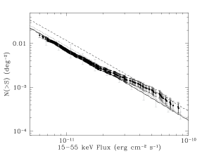
As found by Aird et al. (2015) and Harrison et al. (2016), a XRB model with strong reflection is needed to adequately fit the NuSTAR data. This scenario is illustrated in the figure with the short-dashed line which was computed using the model described in Sect. 2 assuming a fixed $R=1.2$ for all $L_{\mathrm{X}}$ and $z$. This model provides a good description of the NuSTAR counts, but significantly overestimates the Swift-BAT counts at higher fluxes. The right-hand panel of Fig. 1 confirms this conclusion by directly comparing the model predictions to the integrated $N(>S)$ $15$–$55$ keV counts from Ajello et al. (2012).

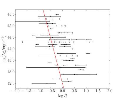
Current observations disfavour a model with a fixed $R$ (e.g., Del Moro et al., 2017), and instead suggest that $R$ is lower for higher-luminosity AGNs (e.g., Zappacosta et al., 2018). To parameterize this luminosity dependence we consider a simple power-law relation,

$$\log R(L_{\mathrm{X}})=a\log L_{\mathrm{X}}+b,$$ (4)

where the $a$ and $b$ are determined by performing a least-squares fit to the $L_{\mathrm{X}}$ and $R$ data provided by Zappacosta et al. (2018). Fitting to the central data points shown in Figure 2 suggests the values $a=-0.29$; $b=12.8$ while fitting to the lower and upper bounds on $\log R$ indicated in the figure give the values $a=-0.26$; $b=10.91$ and $a=-0.29$; $b=13.1$ respectively. However, evolutionary models using $a=-0.29$ and $b\approx 13$ dramatically overestimate the XRB, while the lower bound model predicts it within reasonable error. We thus chose $a=-0.26$ and $b=10.91$ as our luminosity evolutionary model.

Figure 2: Reflection parameter $R$ compared to unabsorbed luminosity $L_{\mathrm{X}}$ for the 63 AGNs presented by Zappacosta et al. (2018). Error bars indicate sources whose value of $R$ is bounded from both above and below, while arrows indicate those whose $R$ is bounded only from above. The red line marks the fit of $\log R(L_{\mathrm{X}})=-0.26\log L_{\mathrm{X}}+10.91$.

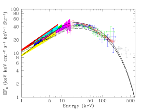
The long-dashed lines in Fig. 1 shows the predicted $8$–$24$ keV $dN/dS$ using this $R$–$L_{\mathrm{X}}$ dependence. This XRB model has uniformly lower values of $R$ than the previous one ($R=1.2$; short-dashed line) and cannot fit the deep NuSTAR counts, but it does provide an excellent fit to the Swift-BAT data. Interestingly, the $R$–$L_{\mathrm{X}}$ relationship was determined by spectral fitting of individual NuSTAR observations from the deep surveys (those selected to have $\log S_{\mathrm{8-24\ keV}}\geq-13.15$; Zappacosta et al. 2018). Perhaps these measurements of $R$ are more accurate than what is inferred by fitting the NuSTAR counts at even fainter fluxes. However, examining the predicted XRB spectrum from these two models (Fig. 3) shows that the weaker reflection strengths predicted by eq. 4 significantly underpredicts the peak of the XRB, while the fixed $R=1.2$ model provides a very reasonable fit to the entire XRB spectrum.

Figure 3: The observed XRB spectrum is compared to four XRB synthesis models described in the text. The line styles denote the four models as in Fig. 1. While both the short-dashed and solid lines provide reasonable fits to the observed XRB spectrum, the model with the consistently weak reflection described by eq. 4 (long-dashed line) significantly underpredicts the data. The colored data and areas denote different measurements of the XRB spectrum: blue - ASCA GIS (Kushino et al., 2002); magenta - RXTE (Revnivtsev et al., 2003); green - XMM-Newton (Lumb et al., 2002); red - BeppoSAX (Vecchi et al., 1999); yellow - ASCA SIS (Gendreau et al., 1995); cyan - XMM-Newton (De Luca & Molendi, 2004); grey data - HEAO-1 (Gruber et al., 1999); blue data - INTEGRAL (Churazov et al., 2007); red data - SWIFT BAT (Ajello et al., 2008); black data - Swift-XRT (Moretti et al., 2009); green data - INTEGRAL (Türler et al., 2010).

Therefore, the $R$–$L_{\mathrm{X}}$ model shown by the long-dashed line must be missing additional reflection strength. Given the good fit to the Swift-BAT data, this additional reflection strength must arise at the fainter fluxes probed by the NuSTAR data which is dominated by AGNs at much higher redshifts than the Swift-BAT sample.

To test the idea of an increasing $R$ with $z$, we calculate a XRB synthesis model with the following simple prescription for $R$,

$$R(L_{\mathrm{X}},z)=\left\{\begin{array}[]{l}R(L_{\mathrm{X}})(1+z)^{\alpha},\ \ z\leq 2\\ R(L_{\mathrm{X}})(1+2)^{\alpha},\ \ z>2\end{array}\right.$$ (5)

where $R(L_{\mathrm{X}})$ is given by eq. 4 with $a=-0.26$ and $b=10.91$, as before. The solid lines in Figs. 1 and 3 show the result of this calculation when $\alpha=2$. This toy model retains the successful fit to the Swift-BAT counts, and provides an adequate description of both the NuSTAR counts and the XRB spectrum. Thus, a reflection fraction that increases with redshift appears to be a viable method to simultaneously account for both the NuSTAR and Swift-BAT $8$–$24$ keV data.

3.1 The Impact of the Compton-thick Fraction

The three XRB models presented above have a Compton-thick fraction set by measurements of the local space density of Compton-thick AGNs (Buchner et al., 2015). However, if this is not a representative value beyond the local Universe, then its possible that simply increasing the Compton-thick fraction may solve the tension between the NuSTAR and Swift-BAT number counts. As the Compton-thick AGN SED peaks at similar energies to the reflection hump (e.g., Akylas et al., 2012), an increase in the Compton-thick fraction will have a similar effect in the XRB model as a larger reflection fraction. To test this possibility, a XRB model was calculated using the $R(L_{X})$ dependence of Eq. 4, but with a Compton-thick fraction $2.76\times$ larger than previously used. This model is shown as the dotted lines in Figs. 1 & 3. The figures show that the larger Compton-thick fraction has a minor impact on the predicted total $8$–$24$ keV number counts. The reason for the modest effect is that the Compton-thick AGN population is still a small component of the total AGN population, comprising only $\approx 2$% of all AGN at a $2$–$10$ keV flux of 10^-14 erg cm^-2 s^-1 after nearly tripling its contribution. Moreover, as seen by the XRB spectrum (Fig. 3), adding even more Compton-thick AGN is not possible, as the enhanced Compton-thick model already skims the top of the observed error-bars. The results of this experiment clearly show that an increase in reflection fraction with $z$ is necessary to resolve the mismatch between the NuSTAR and Swift-BAT number counts.

It is still of interest, however, to determine if the Compton-thick fraction set by the local observed space-density is appropriate at the fainter fluxes probed by NuSTAR. Figure 4 compares the Compton-thick AGN number counts predicted by the four XRB models discussed here to deep measurements from the COSMOS Legacy survey (Ananna et al., 2019; Lanzuisi et al., 2018).

Figure 4: The lines show the predicted Euclidean-normalized differential number counts of Compton-thick AGNs in the $2$–$8$ keV band. The line styles denote the four different XRB models described in the text (see, e.g., Fig. 1). The data points are the observed Compton-thick counts in the $2$–$7$ keV energy band from the COSMOS Legacy survey (Ananna et al., 2019; Lanzuisi et al., 2018). The very small correction between the $2$–$7$ keV and the $2$–$8$ keV energy bands has been omitted for the purpose of this comparison.

The plot clearly shows that the three models with the locally-calibrated Compton-thick fraction substantially underpredicts the COSMOS data, including the two models that satisfactorily describe the NuSTAR $8$–$24$ keV counts. In contrast, the model with the enhanced Compton-thick fraction appears to more accurately describe the Compton-thick counts at these fainter fluxes. This latter model has a Compton-thick fraction of $0.14$ at a $8$–$24$ keV flux of $2.7\times 10^{-14}$ erg cm^-2 s^-1, very similar to what is measured from NuSTAR observations (Masini et al., 2018). The picture that emerges from these experiments is one where both the reflection fraction and possibly the Compton-thick fraction increase with $z$. In the next section, we investigate this possibility further and explore a potential physical explanation for these evolutions.

4 A Physical Model for an Evolving Reflection Fraction

4.1 Model Setup

The previous section showed that a reflection fraction increasing with $z$ can give a XRB model that satisfies both the Swift-BAT and NuSTAR $8$–$24$ keV differential number counts (Fig. 1). However, the values of the reflection fraction predicted by this toy model grow to unreasonably large values at high redshifts (e.g., $R=2.1$ at $z=1$ for $\log(L_{\mathrm{X}}/\mathrm{erg\ s^{-1}})=43$, and this balloons to $R>4$ by $z=2$). Thus, the naïve redshift evolution imposed in Eq. 5 is clearly too extreme, and must be replaced by a physically motivated method for increasing $R$ with $z$ that limits the reflection fraction to more realistic values.

As discussed in Sect. 1, the reflection spectrum in faint AGNs likely originates from reprocessing in the distant gas responsible for AGN obscuration. Recently, Lanz et al. (2019) highlighted the direct connection between $R$ and the obscuring gas in a sample of Swift-BAT AGNs by finding a correlation between the reflected X-ray luminosity (measured by NuSTAR) and the IR luminosity (measured by WISE and Herschel). This result clearly indicates that the X-ray, optical and UV radiation produced by the inner accretion disk is reprocessed by a common structure. Since the obscured fraction of AGNs, $f_{2}$, is observed to increase with $z$ (e.g., Merloni et al., 2014; Liu et al., 2017), then it is natural to expect that the mean $R$ of AGNs will also increase with $z$. In addition, the connection between $R$ and the obscuring gas has been made directly by modeling the stacked spectra of Compton-thin AGNs detected by Swift-BAT and INTEGRAL (Ricci et al., 2011; Vasudevan et al., 2013; Esposito & Walter, 2016). In these studies, stacked spectra separated into $N_{\mathrm{H}}$ bins were found to have different values of $R$ with columns in the range $23\leq\log(N_{\mathrm{H}}/\mathrm{cm^{-2}})\leq 24$ yielding the largest reflection strengths. Such an effect would violate the simplest unified AGN model where all values of $N_{\mathrm{H}}$ co-exist around AGNs, independent of the line-of-sight obscuration. Instead, these results imply that AGNs that are seen through moderate-to-heavy amounts of obscuration exist in fundamentally different environments than those observed through lower $N_{\mathrm{H}}$ columns, and are therefore probing different AGN populations (Draper & Ballantyne, 2010; Buchner et al., 2015). The direct fitting of nearby Swift-BAT AGNs by Lanz et al. (2019) also found that more obscured objects have larger $R$, although the analysis of Ricci et al. (2017) gave the opposite conclusion which could be explained by modeling degeneracies (see Lanz et al. 2019).

The combination of an increasing $f_{2}$ with $z$ and a correlation of $R$ with $N_{\mathrm{H}}$ provides a physical template for the redshift evolution in $R$ that is needed to fit the NuSTAR number counts. From these two pieces of observational evidence a new model for $R(L_{\mathrm{X}},z)$ can be constructed which allows the reflection fraction to increase to higher values of $N_{\mathrm{H}}$:

$$R(N_{\mathrm{H}}[L_{\mathrm{X}},z])=R_{\min}e^{-N_{\mathrm{H}}/N_{\mathrm{H,mid}}}+R_{\max}\left(1-e^{-N_{\mathrm{H}}/N_{\mathrm{H,mid}}}\right),$$ (6)

where $R_{\min}$ and $R_{\max}$ are the lower and upper bounds of $R$ and $N_{\mathrm{H,mid}}$ is the transition point between these values (Figure 5).

Figure 5: An example of the relationship between reflection fraction, $R$, and the absorbing column density, $N_{\mathrm{H}}$ (Eq. 6). The parameters $R_{\min}$ and $R_{\max}$ are fixed at $0.1$ and $1.7$, respectively, and the transition point $N_{\mathrm{H,mid}}$ is set to $10^{23}$ cm^-2.

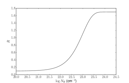
Equation 6 has implicit redshift and luminosity dependencies in the following way. As redshift increases in the XRB model, the fraction of obscured AGNs (i.e., those with $\log(N_{\mathrm{H}}/\mathrm{cm}^{-2})\geq 22$) rises as described by eq. 3. Therefore, the AGN spectra $S_{E}$ that are constructed have a larger and larger proportion of heavily obscured sources, which, as described by eq. 6, is associated with a stronger reflection fraction. Therefore, the spectral model used in the XRB calculation naturally has a larger $R$ at higher redshifts. Likewise, the obscured fraction falls with luminosity in Eq. 3, and so the spectra of more luminous AGNs are constructed with a larger fraction of weakly obscured AGNs which have smaller $R$ (Fig. 5). As a result, the connection between reflection fraction and $N_{\mathrm{H}}$ (eq. 6) naturally describes similar redshift and luminosity evolutions of $R$ as the toy models employed in Sect. 3.

As seen in Fig. 4, a larger Compton-thick fraction at $\log(S_{\mathrm{2-8\ keV}}/\mathrm{erg\ s^{-1}\ cm^{-2}})\approx-14$ may be necessary to match the COSMOS data implying that the evolution of Compton-thick gas around AGNs is decoupled from that of the Compton-thin gas. To parameterize this effect in the XRB model, the Compton-thick fraction is allowed to increase with $z$ as a simple power-law,

$$f_{\mathrm{CT}}(z)=\left\{\begin{array}[]{l}f_{\mathrm{CT,0}}(1+z)^{\gamma},\ \ z\leq 2\\ f_{\mathrm{CT,0}}(1+2)^{\gamma},\ \ z>2\end{array}\right.$$ (7)

where $f_{\mathrm{CT,0}}$ is the local Compton-thick fraction used in Sect. 3 and is determined by matching the measured Compton-thick space density at $z\approx 0$ (Buchner et al., 2015).

4.2 Results

In this section, we compare the results of this physically-motivated XRB model to the NuSTAR and Swift-BAT number counts, the XRB spectrum, and the COSMOS Compton-thick number counts. There are several parameters in this new model (e.g., $R_{\mathrm{min}}$, $R_{\mathrm{max}}$, $\gamma$), but as this is an exploratory model we do not use a fitting method to determine the best-fit values of the parameters. Rather, we explored the effects of each parameter individually until we arrived at a result that best highlighted the properties of the model. Therefore, the parameter values quoted here should be viewed as a starting point from which to develop a more sophisticated model of the evolution of the AGN environment and how it impacts the observed X-ray spectra.

We first consider a model with a fixed Compton-thick fraction (i.e., $\gamma=0$ in eq. 7) in order to isolate the effects of the $R(N_{\mathrm{H}})$ relationship (eq. 6). The predicted $8$–$24$ keV number counts for a model with $R_{\mathrm{min}}=0.1$, $R_{\mathrm{max}}=1.7$ and $N_{\mathrm{H,mid}}=10^{23}$ cm^-2 is shown as the short-dash-long-dash-line in Figure 6. The plot shows that the increase in $R$ with $z$ driven by the changing $f_{2}$ does indeed bend the number counts closer to the NuSTAR data, but falls just below the majority of the NuSTAR error-bars.

Figure 6: The solid line shows the predicted Euclidean-normalized differential $8$–$24$ keV number counts from a $R(N_{\mathrm{H}})$ model (eq. 6) with $R_{\mathrm{min}}=0.1$, $R_{\mathrm{max}}=1.7$, and $N_{\mathrm{H,mid}}=10^{23}$ cm^-2. The model has a Compton-thick evolution parameter $\gamma=0.7$ and requires a more rapid increase in the Type 2 fraction, $\xi=1.3$ (eq. 3) than the models discussed in Sect. 3. A model with no Compton-thick evolution (i.e., $\gamma=0$) is shown as the short-dash-long-dash line and indicates that the $R(N_{\mathrm{H}})$ model may not be enough on its own to account for the NuSTAR number counts. As a point of comparison, the dashed line plots the model from Fig. 1 that lacks any redshift evolution in $R$ or the Compton-thick fraction. The data points are the same as Fig. 1.

At high fluxes the model is nearly identical to the one from Fig. 1 that does not include any redshift evolution (dashed line), but at fainter fluxes the larger fraction of obscured AGNs with larger $R$ values causes the new model to diverge. An interesting aspect of the model is that the factor describing the increase in the Type 2 AGN fraction, $\xi$ (Eq. 3), was increased from $\xi=0.48$ (the value used in Sect. 3) to $\xi=1.3$ in order for the model to lie close to the NuSTAR data. The higher value of $\xi$ ensured there was a significant population of obscured AGNs at higher $z$ which would have larger reflection fractions. Even larger values of $\xi$ were ruled out as those models produced an XRB $2$–$10$ keV slope much harder than observed ($\Gamma=1.45$; e.g., Cappelluti et al. 2017). The value $\xi=1.3$ is higher than what is commonly measured (Hasinger, 2008; Ueda et al., 2014; Liu et al., 2017), but is consistent with the results of Merloni et al. (2014) who found similar values of $\xi$ in two out of three luminosity bins. As pointed out by Liu et al. (2017) it is challenging to accurately measure $\xi$ as the evolution may be luminosity dependent (as found by Merloni et al. 2014) and appears to weaken at $z>2$.

The parameters describing the $R(N_{\mathrm{H}})$ model are constrained by the requirement to fit the Swift-BAT number counts data and to simultaneously reach the NuSTAR number counts. The model shown in Fig. 6 has $R_{\mathrm{min}}=0.1$. Such a low value is required to ensure the fit to the Swift-BAT counts at high fluxes; indeed if $R_{\mathrm{min}}\ga 0.2$ then the fit to those data points is lost. At the high $N_{\mathrm{H}}$ end, $R_{\mathrm{max}}$ is set to $1.7$ to bring the model close to the NuSTAR data. Again, if $R_{\mathrm{max}}$ is increased above $\approx 2$ then the model is pulled away from the Swift-BAT data at high fluxes. Finally, we find $N_{\mathrm{H,mid}}$=10²³ cm^-2 as even a value of $10^{22.5}$ cm^-2 will lead to too strong a reflection signal at high fluxes. To illustrate the $R$ values that result from these parameters Fig. 7 shows the $z$ evolution of the average reflection fraction at four different AGN luminosities, where the average is over the $N_{\mathrm{H}}$ distribution (defined by Burlon et al. 2011) and incorporates the correct $f_{2}$ at the given $L_{\mathrm{X}}$ and $z$ (Eq. 3).

Figure 7: These curves give an indication of the evolution of $R$ with $z$ using the model described by equation 6 with the $N_{\mathrm{H}}$ distribution given by (Burlon et al., 2011) and $f_{2}$ given by equation 3 with $\xi=1.3$. $f_{\mathrm{CT}}$ is held fixed at the $z=0$ value. The evolution is shown at $L_{\mathrm{X}}=10^{43}$ erg s^-1 (dotted line), $L_{\mathrm{X}}=10^{43.5}$ erg s^-1 (dashed line), $L_{\mathrm{X}}=10^{44}$ erg s^-1 (dash-dot line), and $L_{\mathrm{X}}=10^{45}$ erg s^-1 (solid line).

The shape of the curves demonstrate the impact of the various factors described above. At low redshift, more luminous AGNs, which are less obscured than lower luminosity AGNs, have on average consistently weaker values of $R$, as described by eqs. 3 and 6. As redshift increases, the obscured fraction of AGNs with $L_{\mathrm{X}}\ga 10^{43}$ erg s^-1 grows, and, according to eq. 6, more obscured AGNs lead to a larger average $R$. The shape of the $f_{2}$ relation (eq. 3) leads to a faster increase in the average $R$ for high luminosity AGNs than lower luminosity sources. Indeed, in this model, all AGNs have an average $R$ of $\approx 1.3$ by $z=2$.

The short-dash-long-dash line in Figure 8 shows that the integrated XRB spectrum predicted by this model provides a good description of the observed XRB. This contrasts with the previous model from Sect. 3 with no redshift evolution (long dashed line in Fig. 3), and indicates that the magntidue of redshift evolution of $R$ predicted by Eq. 6 is reasonable. However, the growth in $R$ driven by the redshift evolution of the obscured AGN fraction is not enough on its own to account for the NuSTAR $8$–$24$ keV number counts.

Figure 8: As in Fig. 3, but the curves now show models that are based on the $R$-$N_{\mathrm{H}}$ and the $f_{\mathrm{CT}}(z)$ relations (eqs. 6 and 7), with $\gamma=1.7$ (solid line) and $0$ (short-dash-long-dash line). The long-dashed line plots is taken from Fig. 3 and shows a model with no redshift evolution in $R$ or $f_{\mathrm{CT}}$.

Therefore, it is interesting to consider if redshift evolution of the Compton-thick fraction may provide a better fit to the NuSTAR number counts. The solid lines in Figs. 6 and 8 shows that the $R$-$N_{\mathrm{H}}$ connection described by eq. 6 combined with an evolving Compton-thick fraction with $\gamma=0.7$ does improve the description of the $8$–$24$ keV number counts observed by NuSTAR and Swift-BAT. Higher values of $\gamma$ are ruled out as they result in overpredicting the peak of the XRB spectrum. A value of $\gamma=0.7$ implies a Compton-thick fraction at $z=2$ that is $2.2\times$ larger than at $z=0$. The predicted $2$–$8$ keV number counts of Compton-thick AGNs from both this model and the $\gamma=0$ model are compared to the COSMOS Legacy data in Fig. 9 (solid line).

Figure 9: The solid line is the predicted Euclidean-normalized differential number counts of Compton-thick AGNs in the $2$–$8$ keV band from the $R(N_{\mathrm{H}})$ model described in the text. In this model, the Compton-thick AGN fraction grows with redshift as described by Eq. 7 with $\gamma=0.7$. Alternatively, the short-dash-long-dash line plots the same model with no increase in the Compton-thick fraction (i.e., $\gamma=0$). The dashed line and the data points are the same as in Fig. 4. As before, we neglect the very small correction between the $2$–$7$ keV and the $2$–$8$ keV energy bands.

In contrast to the models presented in Sect. 3 (e.g., the dashed line), the Compton-thick number counts predicted by both models provide a decent description of the COSMOS data. Indeed, the Compton-thick fractions at a $8$–$24$ keV flux of $2.7\times 10^{-14}$ erg cm^-2 s^-1 are $0.11$ ($\gamma=0$) and $0.15$ ($\gamma=0.7$). The $\gamma=0$ value is in excellent agreement with the NuSTAR-derived value found by (Masini et al., 2018). The increase in the Compton-thick number counts and fraction in the $R(N_{\mathrm{H}})$ model with no Compton-thick evolution ($\gamma=0$; the short-dash-long-dash line) is a result of the larger $R$ at faint fluxes. Although this model can describe the COSMOS data and the XRB spectrum, Fig. 6 shows that a low-$\gamma$ model would not be able to match the NuSTAR $8$–$24$ keV number counts, requiring larger values of $R$ to compensate which, as described above, would lose the fit to the Swift-BAT number counts. We are forced to conclude that some details of the $R(N_{\mathrm{H}})$ model (eq. 6), which assumes the Burlon et al. (2011) $N_{\mathrm{H}}$ distribution and the $f_{2}(L_{\mathrm{X}})$ relationship (eq. 3), must be revised to self-consistently fit all the data. Nevertheless, it is clear that a XRB model that connects the reflection strength to the changing gas environment around AGNs can successfully describe the hard X-ray survey data produced by NuSTAR and Swift-BAT.

5 Discussion

The results of this paper show that strong redshift evolution in the average AGN reflection fraction appears to be necessary to simultaneously describe the NuSTAR and Swift-BAT $8$–$24$ keV number counts. This effect was not needed in earlier XRB models as survey data at energies $<10$ keV are not very sensitive to changes to $R$, even at very faint flux levels (see Appendix A). The inclusion of a redshift evolution in one of the key XRB parameters presents a challenge to all future XRB synthesis models, as there are many choices on how to parameterize the evolution, and it is likely that other parts of the problem (e.g., the $N_{\mathrm{H}}$ distribution, the Compton-thick fraction) will also vary with $z$. Incorporating all available survey data into a XRB model fit (e.g., Ananna et al., 2019) will be helpful, but may be insufficient without significant improvement in survey data at energies $>10$ keV.

The implications of an evolving $R$ are also significant for our understanding of the changes ongoing within the AGN environment. A changing $R$ means that the amount of high column density gas (i.e., gas with $\log(N_{\mathrm{H}}/\mathrm{cm}^{-2})\geq 23.5$) is evolving over time due to processes within the nuclear environments. The model presented in the previous section required strong reflection only for AGNs with the highest obscuration, as suggested by recent observations (e.g., Esposito & Walter, 2016; Lanzuisi et al., 2018), in complete contrast with the expectations of the orientation-based unification model. Therefore, these highly obscured AGNs are evolving separately from the more weakly obscured and unobscured AGNs and may be connected to changes to the Compton-thick population. When combined with the overall increase in obscured AGNs with redshift (e.g., Merloni et al., 2014; Liu et al., 2017), these considerations all suggest a rich and complex interplay between AGN accretion physics, the obscuration environment, and processes within the host galaxies (e.g., Draper & Ballantyne, 2010; Kocevski et al., 2015; Ricci et al., 2017). Indeed, as both the star-formation rate density and black hole accretion rate density evolve rapidly from $z=0$ to $\approx 2$ (e.g., Madau & Dickinson, 2014), it is perhaps not surprising that other aspects of the AGN environment demonstrate redshift evolution. Therefore, XRB synthesis modeling may need to start including the predictions of physical models of AGN obscuration and its evolution in order to account for all these various effects. Such an exercise could be an important way of discriminating among different AGN environment and evolution models.

An example of this approach was performed by Gohil & Ballantyne (2018) who considered nuclear starburst discs (NSDs) as the source of the obscuring gas around AGNs. These authors used models of star-forming discs at scales of $\sim 1$–$100$ pc from the SMBH (Thompson, Quataert & Murray, 2005; Ballantyne, 2008; Gohil & Ballantyne, 2017), plus observations of the redshift dependence of the gas fraction of galaxies (e.g., Tacconi et al., 2013), to predict the evolving $N_{\mathrm{H}}$ distribution of the obscuring gas. Without any tuning of parameters, the model predicted that $f_{2}$ and $f_{\mathrm{CT}}$ should increase from $z=0$ to $2$ as $(1+z)^{1.2}$ and $(1+z)^{1.45}$, respectively. These dependencies on redshift are interestingly close to the ones ($1.3$ and $0.7$) needed by the XRB synthesis model in the previous section. However, when self-consistently including the reflection strength based on the evolving $N_{\mathrm{H}}$ distribution, Gohil & Ballantyne (2018) found that the NSD model is not able to entirely explain the XRB spectrum, but requires a large fraction of obscured high luminosity AGNs to fit the data. Indeed, the physics of the NSD model limits its applicability to Seyfert-like AGN luminosities (Ballantyne, 2008), but it is an interesting first step on a possible physical approach to XRB modeling.

Compton-thick AGNs have played an important, but poorly understood, role in modeling the XRB. The difficulty in detecting and characterizing these heavily obscured AGNs is well known (e.g., Hickox & Alexander, 2018), especially outside the local Universe. Advances in modeling the X-ray spectra of deeply embedded AGNs (e.g., Murphy & Yaqoob, 2009; Bhayani & Nandra, 2011; Baloković et al., 2018), as well as NuSTAR observations (e.g., Baloković et al., 2014; Annuar et al., 2015; Boorman et al., 2016; Annuar et al., 2017), have allowed progress in identifying Compton-thick sources, but precise measurements of their population statistics remains sparse. Figure 4 demonstrates that a fixed Compton-thick fraction, normalized to the local space density measured by Buchner et al. (2015), can not match the number counts of faint Compton-thick AGNs characterized in the COSMOS Legacy survey, implying that either $f_{\mathrm{CT}}$ or $R$ must evolve in some way. In addition, the previous section found that adding a simple redshift evolution of $f_{\mathrm{CT}}$ (eq. 7) to the $R(N_{\mathrm{H}})$ prescription allowed for the best description of the NuSTAR $8$–$24$ keV number counts. It is possible that the evolution of $R$ and $f_{\mathrm{CT}}$ are physically connected, especially as large $R$ values are associated with significant covering factors of Compton-thick gas. These results support the idea that heavily obscured AGNs may be more commonly associated with specific events in galaxy evolution that funnel large amounts of gas towards the nucleus (e.g., merger events; Draper & Ballantyne 2010; Kocevski et al. 2015).

The approach taken in this paper is to focus on models that can describe the XRB spectrum and $8$–$24$ keV number counts. As seen in Appendix A, changes to the evolution of $R$ and Compton-thick fraction, have a modest impact on the $2$–$10$ keV counts. In addition, we have employed the Ueda et al. (2014) HXLF throughout the calculations, and considered the impact of allowing the parameters describing AGN spectra to vary with redshift. An alternative approach, recently pursued by Ananna et al. (2019), considers a small number of fixed AGN spectral models, but modifies the HXLF in order to fit the X-ray survey data. While it is important that the measured HXLFs be continuously improved, the observed increase in $f_{2}$ (e.g., Liu et al., 2017), the connection between $N_{\mathrm{H}}$ and $R$ (e.g., Lanz et al., 2019), and the increasing evidence for fundamental physical connections between the AGN and its environment (e.g., Ricci et al., 2017), all strongly suggest that the observed AGN X-ray SED will be functions of both redshift and luminosity that should be considered in future XRB synthesis models.

6 Conclusions

Since their advent in the mid-1990s, XRB synthesis modeling has been an important component in the study of the demographics and evolution of AGNs. The results of this paper, which presents evidence that the reflection fraction $R$ evolves with $z$, implies that XRB synthesis modeling, when combined with X-ray surveys at energies $>10$ keV, should now be considered as a method to explore the evolution of AGN physics in addition to their demographics. The dependence of $R$ with physical properties such as the $N_{\mathrm{H}}$ distribution and the AGN luminosity means that the evolution of $R$ can help distinguish between different physical models of the origin of the obscuring gas and its connection to processes in the AGN host galaxy. As both the photon-index and high-energy cutoff of the AGN power-law also depend on the fundamental physics of accretion discs, future XRB synthesis models have the potential to reveal the evolution of many aspects of AGN physics throughout cosmic time.

The results of this paper also provide a striking illustration of the potential of future hard X-ray surveys in understanding the evolution of the physical environment of AGNs. Only surveys at X-ray energies $>10$ keV will be sensitive enough to the effects of evolution in $R$ and $E_{\mathrm{cut}}$ to constrain models of AGN evolution in a rigorous way. The hard X-ray band is also crucial to properly model the complex SEDs of Compton-thick AGNs (e.g., Baloković et al., 2018). Therefore, future X-ray mission concepts that include hard X-ray capabilities (e.g., HEX-P, STROBE-X; Ray et al. 2018) will be crucial in allowing XRB synthesis modeling to reach its potential.

Appendix A The View in the 2–10 keV Band

The AGN number counts in the $2$–$10$ keV energy band have been probed to remarkable depths by both XMM-Newton and Chandra (e.g., Liu et al., 2017), but these data are not highly sensitive to the high-energy properties of AGN spectra even at very faint fluxes. This is illustrated in Figure 10 which plots the Euclidean-normalized integrated $N(>S)$ $2$–$10$ keV number counts predicted by the four models described in Sect. 3.

Figure 10: The Euclidean-normalized integrated AGN number counts in the $2$–$10$ keV band predicted by the four XRB synthesis models described in Sect. 3 and in Fig. 1. The solid points are the counts measured by the Chandra-COSMOS survey (Civano et al., 2016) while the higher-flux data are from the XMM-Newton measurements of Mateos et al. (2008). These two datasets capture the spread of the number counts meaurements at intermediate fluxes (Civano et al., 2016). Despite the differences in the value and evolution of $R$, the different XRB models are all consistent with the current measurements. Therefore, without a significant decrease in the spread of the number count measurements at $S\approx 10^{-14}$ erg cm^-2 s^-1 the $2$–$10$ keV band is not sensitive enough to constrain or test for significant variations of $R$ with either $L_{\mathrm{X}}$ or $z$.

The four models provide a good description of number counts measurements from Chandra and XMM-Newton (Mateos et al., 2008; Civano et al., 2016). These datasets illustrate the spread of number counts measurements found from a number of surveys (Civano et al., 2016). The four models are virtually indistinguishable at $S\ga 10^{-13}$ erg cm^-2 s^-1. At faint fluxes ($S\la 10^{-15}$ erg cm^-2 s^-1) the model with the boosted Compton-thick fraction (dotted line; Sect. 3.1) begins to seperate from the other models, but characterizing Compton-thick AGNs at such faint fluxes is a significant challenge. At intermediate fluxes (e.g., $S\approx 10^{-14}$ erg cm^-2 s^-1) the models seperate into two groups: the number counts predicted by the fixed-$R$ (short-dashed line) and the strongly-evolving $R$ (solid line) models trace the upper end of the data envelope, while the low-$R$ models (long dashed and dotted lines) track the lower range. Therefore, use of the $2$–$10$ keV band to distinguish between different luminosity and $z$ evolutions of $R$ would require a very significant decrease in the spread of the number count measurements. This result emphasizes the importance of sensitive hard X-ray measurements by NuSTAR and other future missions, as only surveys at energies $\ga 10$ keV will more easily be able to detect aspects of AGN evolution connected to reflection and the high-energy cutoff.

References

- Aird et al. (2015) Aird J., et al., 2015, ApJ, 815, 66
- Ajello et al. (2008) Ajello M., et al., 2008, ApJ, 689, 666
- Ajello et al. (2012) Ajello M., Alexander D.M., Greiner J., Madejski G.M., Gehrels N., Burlon, D., 2012, ApJ, 749, 21
- Ananna et al. (2019) Ananna T.T., et al., 2019, ApJ, 871, 240
- Annuar et al. (2015) Annuar A., et al., 2015, ApJ, 815, 36
- Annuar et al. (2017) Annuar A., et al., 2017, ApJ, 836, 165
- Arnaud (1996) Arnaud K.A., 1996, in Jacoby G., Barnes J., eds, Astronomical Data Analysis Software and Systems V, ASP Conf. Ser. Vol. 101, 17
- Akylas & Georgantopoulos (2019) Akylas A., Georgantopoulos I., 2019, A&A, in press (arXiv:1902.05137)
- Akylas et al. (2012) Akylas A., Georgakakis A., Georgantopoulos I., Brightman M., Nandra, K., 2012, A&A, 546, A98
- Baloković et al. (2014) Baloković M., et al., 2014, ApJ, 794, 111
- Baloković et al. (2018) Baloković M., et al., 2018, ApJ, 854, 42
- Ballantyne et al. (2006) Ballantyne D.R., Everett J.E., Murray, N., 2006, ApJ, 639, 740
- Ballantyne et al. (2011) Ballantyne D.R., Draper A.R., Madsen K., Rigby J.R., Treister, E., 2011, ApJ, 736, 56
- Ballantyne (2008) Ballantyne D.R., 2008, ApJ, 685, 787
- Ballantyne (2014) Ballantyne D.R., 2014, MNRAS, 437, 2845
- Bhayani & Nandra (2011) Bhayani S., Nandra, K., 2011, MNRAS, 416, 629
- Boorman et al. (2016) Boorman P.G. et al., 2016, ApJ, 833, 245
- Brightman & Nandra (2011) Brightman M., Nandra K., 2011, MNRAS, 413, 1206
- Buchner et al. (2015) Buchner J., et al., 2015, ApJ, 802, 89
- Burlon et al. (2011) Burlon D., Ajello M., Greiner J., Comastri A., Merloni A., Gehrels N., 2011, ApJ, 728, 58
- Cappelluti et al. (2017) Cappelluti N., et al., 2017, ApJ, 837, 19
- Churazov et al. (2007) Churazov E. et al., 2007, A&A, 467, 529
- Civano et al. (2015) Civano F., et al., 2015, ApJ, 808, 185
- Civano et al. (2016) Civano F., et al., 2016, ApJ, 819, 62
- Comastri et al. (1995) Comastri A., Setti G., Zamorani G., Hasinger, G., 1995, A&A, 296, 1
- de la Calle Pérez et al. (2010) de la Calle Pérez I. et al., 2010, A&A, 524, A50
- Del Moro et al. (2017) Del Moro A., et al., 2017, ApJ, 849, 57
- De Luca & Molendi (2004) De Luca A., Molendi, S., 2004, A&A, 419, 837
- Draper & Ballantyne (2009) Draper A.R., Ballantyne D.R., 2009, ApJ, 707, 778
- Draper & Ballantyne (2010) Draper A.R., Ballantyne D.R., 2010, ApJ, 715, L99
- Esposito & Walter (2016) Esposito V., Walter R., 2016, A&A, 590, A49
- Galeev et al. (1979) Galeev A.A., Rosner, R., Vaiana G.S., 1979, ApJ, 229, 318
- García & Kallman (2010) García J., Kallman T.R., 2010, ApJ, 718, 695
- Gendreau et al. (1995) Gendreau K.C. et al., 1995, PASJ, 47, L5
- Georgakakis et al. (2017) Georgakakis A. et al., 2017, MNRAS, 469, 3232
- George & Fabian (1991) George I.M., Fabian A.C., 1991, MNRAS, 249, 352
- Gilli et al. (2007) Gilli R., Comastri A., Hasinger G., 2007, A&A, 463, 79
- Gohil & Ballantyne (2017) Gohil R., Ballantyne D.R., 2017, MNRAS, 468, 4944
- Gohil & Ballantyne (2018) Gohil R., Ballantyne D.R., 2018, MNRAS, 475, 3543
- Gruber et al. (1999) Gruber D.E., Matteson J.L., Peterson L.E., Jung, G.V., 1999, ApJ, 520, 124
- Haardt & Maraschi (1991) Haardt F., Maraschi L., 1991, ApJ, 380, L51
- Haardt & Maraschi (1993) Haardt F., Maraschi L., 1993, ApJ, 413, 507
- Haardt et al. (1994) Haardt F., Maraschi L., Ghisellini G., 1994, ApJ, 432, L95
- Harrison et al. (2013) Harrison F.A., et al., 2013, ApJ, 770, 103
- Harrison et al. (2016) Harrison F.A. et al., 2016, ApJ, 831, 185
- Hasinger (2008) Hasinger G., 2008, A&A, 490, 905
- Hickox & Alexander (2018) Hickox R.C., Alexander D.M., 2018, ARA&A, 56, 625
- Hopkins et al. (2006) Hopkins P.F., Hernquist L., Cox, T.J., Di Matteo T., Robertson B., Springel V., 2006, ApJS, 163, 1
- Iwasawa & Taniguchi (1993) Iwasawa K., Taniguchi Y., 1993, ApJ, 413, L15
- Kara et al. (2016) Kara E., Alston W.N., Fabian A.C., Cackett E.M., Uttley P., Reynolds C.S., Zoghbi A., 2016, MNRAS, 462, 511
- Kocevski et al. (2015) Kocevski D., et al., 2015, ApJ, 814, 104
- Krivonos et al. (2010) Krivonos R., Tsygankov S., Revnivtsev M., Grebenev S., Churazov E., Sunyaev R., 2010, A&A, 523, A61
- Kushino et al. (2002) Kushino A., Ishisaki Y., Morita U., Yamasaki N.Y., Ishida M., Ohashi T., Ueda, Y., 2002, PASJ, 54, 327
- La Franca et al. (2005) La Franca F. et al., 2005, ApJ, 635, 864
- Lansbury et al. (2017) Lansbury G., et al., 2017, ApJ, 836, 99
- Lanz et al. (2019) Lanz L., et al., 2019, ApJ, 870, 26
- Lanzuisi et al. (2018) Lanzuisi G., et al., 2018, MNRAS, 480, 2578
- Liu et al. (2017) Liu T., et al., 2017, ApJS, 232, 8
- Lumb et al. (2002) Lumb D.H., Warwick R.S., Page M., De Luca, A., 2002, A&A, 389, 93
- MacLeod et al. (2015) MacLeod C.L., et al., 2015, ApJ, 806, 258
- Madau & Dickinson (2014) Madau P., Dickinson M., 2014, ARA&A, 52, 415
- Mainieri et al. (2007) Mainieri V., et al., 2007, ApJS, 172, 368
- Mantovani et al. (2016) Mantovani G., Nandra K., Ponti, G., 2016, MNRAS, 458, 4198
- Marchesi et al. (2016) Marchesi S., et al., 2016, ApJ, 830, 100
- Masini et al. (2018) Masini A., et al., 2018, ApJS, 235, 17
- Mateos et al. (2008) Mateos S., et al., 2008, A&A, 492, 51
- Matt et al. (1991) Matt G., Perola G.C.,Piro, L., 1991, A&A, 247, 25
- Merloni et al. (2014) Merloni A., et al., 2014, MNRAS, 437, 3550
- Moretti et al. (2009) Moretti A. et al., 2009, A&A, 493, 501
- Morrison & McCammon (1983) Morrison R., McCammon D., 1983, ApJ, 270, 119
- Mullaney et al. (2015) Mullaney J.R., et al., 2015, ApJ, 808, 184
- Murphy & Yaqoob (2009) Murphy K.D., Yaqoob T., 2009, MNRAS, 397, 1549
- Nandra (2006) Nandra K., 2006, MNRAS, 368, L62
- Nandra et al. (2007) Nandra K., O’Neill P.M., George I.M., Reeves J.N., 2007, MNRAS, 382, 194
- Patrick et al. (2012) Patrick A.R., Reeves J.N., Porquet D., Markowitz A.G., Braito V., Lobban, A.P., 2012, MNRAS, 426, 2522
- Ray et al. (2018) Ray P., et al., 2018, Proceedings of the SPIE, 10699, 1069919
- Reis & Miller (2013) Reis R.C., Miller J.M., 2013, ApJ, 769, L7
- Revnivtsev et al. (2003) Revnivtsev M., Gilfanov M., Sunyaev R., Jahoda K., Markwardt C., 2003, A&A, 411, 329
- Ricci et al. (2011) Ricci C., Walter R., Courvoisier T.J.-L., Paltani S., 2011, A&A, 532, A102
- Ricci et al. (2013) Ricci C., Paltani S., Ueda Y., Awaki H., 2013, MNRAS, 435, 1840
- Ricci et al. (2014) Ricci C., Ueda Y., Paltani S., Ichikawa K., Gandhi P., Awaki H., 2014, MNRAS, 441, 3622
- Ricci et al. (2015) Ricci C., Ueda Y., Koss M.J., Trakhtenbrot B., Bauer F.E., Gandhi P., 2015, ApJ, 815, 13
- Ricci et al. (2017) Ricci C., et al., 2017, ApJS, 233, 17
- Ricci et al. (2018) Ricci C., et al., 2018, MNRAS, 480, 1819
- Ross & Fabian (1993) Ross R.R., Fabian A.C., 1993, MNRAS, 261, 74
- Ross et al. (1999) Ross R.R., Fabian A.C., Young A.J., 1999, MNRAS, 306, 461
- Ross & Fabian (2005) Ross R.R., Fabian A.C., 2005, MNRAS, 358, 211
- Shu et al. (2010) Shu X.W., Yaqoob T., Wang, J.X., 2010, ApJS, 187, 581
- Shu et al. (2011) Shu X.W., Yaqoob T., Wang, J.X., 2011, ApJ, 738, 147
- Shu et al. (2012) Shu X.W., Wang J.X., Yaqoob T., Jiang P., Zhou Y.Y., 2012, ApJ, 744, L21
- Tacconi et al. (2013) Tacconi L.J., et al., 2013, ApJ, 768, 74
- Thompson, Quataert & Murray (2005) Thompson T.A., Quataert E., Murray N., 2005, ApJ, 630, 167
- Tortosa et al. (2018) Tortosa A., Bianchi S., Marinucci A., Matt G., Petrucci P.O., 2018, A&A, 614, A37
- Treister & Urry (2005) Treister E., Urry C.M., 2005, ApJ, 630, 115
- Treister et al. (2009) Treister E., Urry C.M., Virani S., 2009, ApJ, 696, 110
- Türler et al. (2010) Türler M., Chernyakova M., Courvoisier T. J.-L., Lubiński P., Neronov A., Produit N., Walter, R., 2010, A&A, 512, A49
- Ueda et al. (2003) Ueda Y., Akiyama M., Ohta K., Miyaji T., 2003, ApJ, 598, 886
- Ueda et al. (2014) Ueda Y., Akiyama M., Hasinger G., Miyaji T., Watson, M.G., 2014, ApJ, 786, 104
- Vasudevan et al. (2013) Vasudevan R.V., Mushotzky R.F., Gandhi P., 2013, ApJ, 770, L37
- Vecchi et al. (1999) Vecchi A., Molendi S., Guainazzi M., Fiore F., Parmar A. 1999, A&A, 349, L73
- Walton et al. (2013) Walton D.J., Nardini E., Fabian A.C., Gallo L.C., Reis, R.C., 2013, MNRAS, 428, 2901
- Yaqoob (2012) Yaqoob T., 2012, MNRAS, 423, 3360
- Zappacosta et al. (2018) Zappacosta L., et al., 2018, ApJ, 854, 33
- Zoghbi et al. (2013) Zoghbi A., Reynolds C., Cackett E.M., Miniutti G., Kara E., Fabian A.C., 2013, ApJ, 767, 121