“TNOs are Cool”: A survey of the trans-Neptunian region

Abstract

Context. A group of trans-Neptunian objects (TNO) are dynamically related to the dwarf planet 136108 Haumea. Ten of them show strong indications of water ice on their surfaces, are assumed to have resulted from a collision, and are accepted as the only known TNO collisional family. Nineteen other dynamically similar objects lack water ice absorptions and are hypothesized to be dynamical interlopers.

Aims. We have made observations to determine sizes and geometric albedos of six of the accepted Haumea family members and one dynamical interloper. Ten other dynamical interlopers have been measured by previous works. We compare the individual and statistical properties of the family members and interlopers, examining the size and albedo distributions of both groups. We also examine implications for the total mass of the family and their ejection velocities.

Methods. We use far-infrared space-based telescopes to observe the target TNOs near their thermal peak and combine these data with optical magnitudes to derive sizes and albedos using radiometric techniques. Using measured and inferred sizes together with ejection velocities we determine the power-law slope of ejection velocity as a function of effective diameter.

Results. The detected Haumea family members have a diversity of geometric albedos $\sim$ 0.3-0.8, which are higher than geometric albedos of dynamically similar objects without water ice. The median geometric albedo for accepted family members is $p_{V}=0.48_{-0.18}^{+0.28}$, compared to 0.08${}_{-0.05}^{+0.07}$ for the dynamical interlopers. In the size range $D=175-300$ km, the slope of the cumulative size distribution is $q$=3.2${}_{-0.4}^{+0.7}$ for accepted family members, steeper than the $q$=2.0$\pm$0.6 slope for the dynamical interlopers with D$<$500 km. The total mass of Haumea’s moons and family members is 2.4% of Haumea’s mass. The ejection velocities required to emplace them on their current orbits show a dependence on diameter, with a power-law slope of 0.21-0.50.

1 Introduction

Over the past 25 years, a large number of icy bodies have been discovered orbiting beyond Neptune in the outer solar system. These trans-Neptunian objects (TNO) are material left behind from the formation of our solar system, and contain a wealth of information on how the planets migrated to their current orbits. In addition, they likely constitute the principal source of short-period comets, through their daughter population, the centaurs (Levison & Duncan 1997; Horner et al. 2004). The dwarf planet 136108 Haumea is one of the largest TNOs. With a volume-equivalent diameter of $D$$\sim$1600 km (Ortiz et al. 2017), its size is between the category of Pluto and Eris (D$>$2300 km, Sicardy et al. 2011) and the other largest TNOs 2007 OR₁₀, Makemake, Quaoar, and Sedna (Ortiz et al. 2012a; Santos-Sanz et al. 2012; Braga-Ribas et al. 2013; Pál et al. 2012, 2016). While mutual collisions have shaped the size distribution of small and moderate sized TNOs (diameter $<$50-100 km) larger TNOs have generally not been eroded by disruptive collisions, so their size distribution is thought to reflect the accretion process (Davis & Farinella 1997). Large objects usually experience impact cratering instead of disruptive collisions. However, the large object Haumea may be an exception to this rule as it is hypothesized to be the parent body of the so-far only identified collisional family among TNOs (Brown et al. 2007; Levison et al. 2008b; Marcus et al. 2011). It has a short rotation period of 3.92 h (Rabinowitz et al. 2006) close to the calculated and observed spin breakup limit of TNOs (Leinhardt et al. 2010; Thirouin et al. 2010) as well as a rotationally deformed shape and a ring (Ortiz et al. 2017), which all are unique properties among the $D$$\geq$1000 km TNOs. The geometric albedo of Haumea ($\sim$0.5) due to water ice is less than the albedos of Pluto and Eris, which have volatile ices, whereas smaller TNOs with measured albedos available in the literature have geometric albedos $\lesssim$0.4 (e.g. Lacerda et al. 2014a). All TNOs with $D$$\geq$1000 km for which spectra have been obtained feature methane ice on their surfaces, except Haumea which has only water ice (Barucci et al. 2011, and references cited therein). Spectral modelling suggests a 1:1 mixture of crystalline and amorphous water ice on Haumea’s surface and that it is depleted in carbon-bearing materials besides CH₄ compared to most other TNOs (Pinilla-Alonso et al. 2009).

Brown et al. (2007) noted that a group of five TNOs including Haumea that have very deep near-infrared (NIR) water ice absorption features are also dynamically clustered, that is, they have similar proper orbital elements. Ragozzine & Brown (2007) listed objects with low velocities relative to Haumea’s supposed collisional location. About one third of them have strong water ice features and so are family members. At that time it was also known that the larger moon Hi’iaka has a strong water ice absorption in its spectrum (Barkume et al. 2006). Brown et al. (2007) proposed that the group of five objects are fragments of Haumea’s ice mantle disrupted by a collision with an object 60% of the size of proto-Haumea. Such a collision may have removed $\sim$20% of Haumea’s initial mass. To date most authors have accepted the hypothesis that only those TNOs which both (i) are in the dynamical cluster and (ii) have strong water ice absorptions are members of the family. While some other TNOs have water ice absorptions (Brown et al. 2012), they are weaker, and those TNOs are not part of the dynamical cluster. One member of the dynamical cluster is the $D$$\sim$300 km TNO 2002 TX₃₀₀ with high geometric albedo of 0.88 (Elliot et al. 2010), which has been identified as one of the Haumea family members as it has strong water ice absorption bands (Licandro et al. 2006). The whole population of TNOs in general has a wide range of colours (e.g. Doressoundiram et al. 2008; Hainaut et al. 2012) but all the Haumea family members show neutral colours. Spectroscopic data is not available for all potential Haumea family members and new techniques to detect water ice signatures with NIR photometry have been developed (e.g. Snodgrass et al. 2010; Trujillo et al. 2011) in order to infer family membership. The number of spectroscopically or photometrically confirmed members is currently ten in addition to Haumea and its two moons Hi’iaka and Namaka (Brown et al. 2007; Ragozzine & Brown 2007; Schaller & Brown 2008; Snodgrass et al. 2010; Trujillo et al. 2011; Fraser & Brown 2009).

The semi-major axes of the orbits of the Haumea family members are 42.0$<$a$<$44.6 AU, their orbital inclinations are 24.2$\degr$$<$$i$$<$29.1$\degr$, and their eccentricities are 0.11$<$$e$$<$0.17. For all the members in the dynamical cluster the orbital elements are 40$<$a$<$47 AU, 22$\degr$$<$i$<$31$\degr$ and 0.06$<$e$\leq$0.2. Haumea has a more eccentric orbit than the rest of the family with $e$=0.20. It is currently in a 12:7 mean motion resonance with Neptune (Lykawka & Mukai 2007), and Brown et al. (2007) suggest that its current proper orbital elements have changed since the presumed collision event. Lykawka & Mukai (2007) indicated that 19308 (1996 TO₆₆) is in a 19:11 resonance with Neptune but this resonance membership could not be confirmed by later works (e.g. Lykawka et al. 2012). Unless in mean motion resonance, the confirmed family members are in the dynamically hot sub-population of classical Kuiper belt objects (CKBO) according to the Gladman et al. (2008) classification system, but are classified as scattered-extended in the Deep Ecliptic Survey classification system (Elliot et al. 2005). Collisions in the present classical transneptunian belt are very unlikely and the family would probably have been dispersed during the chaotic migration phase of planets if it formed before the dynamically hot CKBOs had evolved to their current orbits as predicted by the Nice model (e.g. Levison et al. 2008a). Based on calculations of collision probabilities, Levison et al. (2008b) showed that over 4.6 Ga a collision leading to the formation of one family is likely if both the colliding objects were scattered-disk objects on highly eccentric orbits, and that it could result in a CKBO-type orbit after the collision.

One of the biggest challenges to the collisional disruption formation mechanism is that the objects with strong water ice features are tightly clustered, having a velocity dispersion clearly smaller ($\sim$20 $ms^{-1}$–300 $ms^{-1}$, Ragozzine & Brown 2007) than the escape velocity of Haumea ($\sim$900 ms^-1). This is unusual for fragments of a disruptive impact (Schlichting & Sari 2009). Various models have been proposed to explain the small velocity dispersion: a grazing impact of two equal-sized objects followed by merger (Leinhardt et al. 2010); disruption of a large satellite of the proto-Haumea (Schlichting & Sari 2009); and rotational fission (Ortiz et al. 2012b). While the collisional models can explain the low velocity dispersion of the canonically-defined family members, another possibility is that the family is more extensive than has been assumed based on NIR spectral evidence. A recent review of collisional mechanisms has been presented by Campo Bagatin et al. (2016). They also propose the alternative that Haumea together with its moons was formed independently of the family of objects presumed to form the rest of the Haumea family, that is, that there were two parent bodies on close orbits. The different water ice fractions on the surfaces of Haumea compared to the family average found by Trujillo et al. (2011) would be compatible with this hypothesis. The inverse correlation of size (via its proxy, the absolute magnitude) with the presence of water ice was explained by Trujillo et al. (2011) to be caused by two possibilities: smaller objects having a larger fraction of ice on their surfaces or smaller objects having a larger grain size.

In order to quantify the albedos and sizes of Haumea family members we use all available far-infrared observations. Six of the confirmed family members have been observed with the Herschel Space Observatory (Pilbratt et al. 2010) and four of them have also Spitzer Space Telescope observations. The radiometric results of five confirmed family members 19308 (1996 TO₆₆), 24835 (1995 SM₅₅), 120178 (2003 OP₃₂), 145453 (2005 RR₄₃), and 2003 UZ₁₁₇ are new in this work. We describe these Herschel and Spitzer observations as well as optical absolute magnitudes in Sect. 2 and present the radiometric analysis in Sect. 3. We discuss the implication to the Haumea family in Sect. 4 and make conclusions in Sect. 5.

2 Observations and auxiliary data

2.1 Herschel observations

The observations of the Haumea family with the Herschel Space Observatory were part of the Open Time Key Program “TNOs are Cool” (Müller et al. 2009), which used in total about 400 hours of observing time during the Science Demonstration Phase and Routine Science Phases to observe 132 targets. Haumea itself was observed extensively, more than ten hours with two photometric instruments, the Photodetector Array Camera and Spectrometer (PACS) at 70, 100, and 160 $\mu m$ (Poglitsch et al. 2010) and the Spectral and Photometric Imaging Receiver (SPIRE) at 250, 350, and 500 $\mu m$ (Griffin et al. 2010). The thermal light curve of the system of Haumea and its moons were analysed by Lellouch et al. (2010) and Santos-Sanz et al. (2017) and the averaged multi-band observations by PACS and SPIRE in Fornasier et al. (2013). Six confirmed Haumea family members were observed by Herschel as part of this work (Table 1) using a total of about 12 hours. In addition, eight probable dynamical interlopers were analysed in previous works from “TNOs are Cool” and one of them (1999 KR₁₆) has updated flux densities given in Table 1. The previously unpublished Herschel observations of the dynamical interloper 1999 CD₁₅₈ are part of this work.

The Herschel/PACS observations of the Haumea family were planned in the same way as other observations in the key programme (e.g. Vilenius et al. 2012). The instrument was continuously sampling while the telescope moved in a pattern of parallel scan legs, each 3$\arcmin$ in length, around the target coordinates. We had checked the astrometric uncertainty of the coordinates with the criterion that the 3$\sigma$ positional uncertainty was less than 10$\arcsec$. Each PACS observation (identified by “OBSID”) produced a map that was the result of repeating the scan pattern several times. This repetition factor was a free parameter in the planning of the duration of observations. In the beginning of the Routine Science Phase of Herschel in the first half of 2010 (Table 1), we used repetition factors of two to three based on detecting thermal emission of an object assuming it has a geometric albedo of 0.08. Later in 2011 we used longer observing time with repetition factors of four to five to take into account the possible high albedo of Haumea family members as indicated by Elliot et al. (2010) for 2002 TX₃₀₀ because higher geometric albedo at visible wavelengths means less emission in the far-infrared wavelengths.

We used the Herschel Interactive Processing Environment (HIPE, version 9.0 / CIB 2974) to produce Level 2 maps with the scan map pipeline script, with TNO-specific parameters given in Kiss et al. (2014). This script projects pixels of the original frames produced by the detector into pixels of a sub-sampled output map. Each target was observed with the same sequence of individual OBSIDs at two epochs separated by about one day so that the target had moved by 25-50$\arcsec$. We applied background subtraction using the double-differential technique (Kiss et al. 2014) to produce final maps from individual OBSIDs. We used standard aperture photometry techniques to determine flux densities. The uncertainties were determined by implanting 200 artificial sources in the vicinity of the real source and calculating the standard deviation of flux densities determined from these artificial sources. The upper limits in Table 1 are 1$\sigma$ noise levels of the final map determined by this artificial source technique. The colour corrections were calculated in the same iterative way as in Vilenius et al. (2012) and they amount to a few percent. The uncertainties include the absolute calibration uncertainty, which is 5% in all PACS bands (Balog et al. 2014).

The previously published Herschel observations of 1999 KR₁₆ (Santos-Sanz et al. 2012) have been re-analysed in this work (Table 1). Santos-Sanz et al. (2012) used the super-sky subtraction method (Stansberry et al. 2008) and reported flux densities of 5.7$\pm$0.7 / 3.5$\pm$1.0 / 4.6$\pm$2.2 mJy, which were ”mutually inconsistent” as shown in their Fig. 1. In our updated analysis we found out that there was a background source near the target located in such a way that the double-differential technique (Kiss et al. 2014) did not fully remove it. We consider the visit 2 images as contaminated and use only visit 1. Moreover, we consider the 160 $\mu$m band an upper limit.

Table 1: Herschel observations and monochromatic flux densities of six unpublished and two reanalysed targets. Targets 2002 TX₃₀₀ (Lellouch et al. 2013) and 1999 KR₁₆ (Santos-Sanz et al. 2012) have been reanalysed and their flux densities updated in this work.

Target	1st OBSIDs	Dur.	Mid-time	$r$	$\Delta$	$\alpha$	Flux densities (mJy)
	of visit 1/2	(min)		(AU)	(AU)	(°)	$70\,\mathrm{\mu m}$	$100\,\mathrm{\mu m}$	$160\,\mathrm{\mu m}$
1995 SM$_55$	1342190925/…0994	73.1	2010-Feb-22 11:58	38.62	38.99	1.37	$<$1.7	$<$1.7	$<$2.7
2005 RR$_43$	1342190957/…1033	73.1	2010-Feb-23 00:16	38.73	38.88	1.45	$2.6\pm 1.8$	$4.6\pm 2.4$	$<$2.8
2003 UZ$_117$	1342190961/…1037	109.3	2010-Feb-23 01:07	39.27	39.50	1.41	$2.0\pm 1.6$	$<$2.2	$<$2.3
2003 OP$_32$	1342197669/…7721	75.7	2010-Jun-03 20:31	41.53	41.31	1.39	$1.7\pm 1.5$	$<$2.1	$<$4.1
2002 TX$_300$	1342212764/…2802	188.5	2011-Jan-17 03:46	41.68	41.76	1.36	$1.2\pm 1.1$	$<$2.8	$<$4.1
1996 TO$_66$	1342222430/…2481	188.5	2011-Jun-10 11:25	46.92	47.34	1.14	$<$1.2	$<$1.3	$<$2.9
1999 CD$_158$	1342206024/…6060	150.9	2010-Oct-08 05:01	47.40	47.83	1.09	$<$1.3	$<$1.6	$<$2.1
1999 KR$_16$	1342212814/…3071	188.5	2011-Jan-18 06:14	35.76	36.06	1.51	4.2 $\pm$1.1	6.9 $\pm$2.2	$<$4.5

2.2 Spitzer observations

Four members of the Haumea family were observed using the Multiband Imaging Photometer for Spitzer (MIPS, Rieke et al. 2004) aboard the Spitzer Space Telescope (Werner et al. 2004). These observations utilized MIPS’ chop-nod photometric mode using the dedicated chopper mirror and spacecraft slews as nods, and the spectral channels centred at $24\ \mathrm{\mu m}$ (effective monochromatic wavelength: $23.68\ \mathrm{\mu m}$) and $70\ \mathrm{\mu m}$ ($71.42\ \mathrm{\mu m}$). There is strong spectral overlap between the 70-micron channels of MIPS and PACS.

We reanalysed (Mueller et al., in prep.) the MIPS observations using the methods described by Stansberry et al. (2007, 2008) and Brucker et al. (2009), along with recent ephemeris information. Targets 2002 TX₃₀₀ and 2003 OP₃₂ were observed more than once and a background-subtraction method was used to produce combined maps. The individual visits were made within about two days of the first visit of the observed target. Flux densities were determined from the resulting mosaics using aperture photometry. Flux uncertainties were estimated using two techniques, one using a standard sky annulus, one using multiple sky apertures.

None of the Haumea family members were detected by Spitzer. Our analysis provides upper flux limits (see Table 2). We provide tighter limits based on new reduction of the data on the non-detection of 2002 TX₃₀₀ than a previous analysis by Stansberry et al. (2008); the remaining observations have not been published so far.

Table 2: Spitzer/MIPS observations.

Target	PID	Mid-time	$r$	$\Delta$	$\alpha$	MIPS $24\ \mathrm{\mu m}$ band		MIPS $70\ \mathrm{\mu m}$ band
			(AU)	(AU)	(°)	Dur. (min)	F24 (mJy)	Dur. (min)	F70 (mJy)
1995 SM55	55	2006-Feb-18 16:27	38.93	39.03	1.47	16.5	$<$0.045	22.4	$<$3.75
1996 TO66	55	2004-Dec-26 10:22	46.40	46.22	1.23	…	…	44.8	$<$4.66
2002 TX300	3283	2004-Dec-28 02:04	40.98	40.73	1.37	5.3	$<$0.025	5.6	$<$5.59
2003 OP32	30081	2006-Dec-07 00:49	41.19	41.15	1.41	57.5	$<$0.015	33.6	$<$4.80
1999 KR16	55	2006-Feb-18 05:51	36.73	36.65	1.56	…	…	44.8	$<$2.24

2.3 Optical data

In the radiometric method we simultaneously fit flux densities and absolute magnitude $H_{\mathrm{V}}$ to the model of emitted flux and to the optical constraint, respectively (Equations 1 and 2 in Sect. 3.1). Generally, an accurate $H_{\mathrm{V}}$ affects mainly the accuracy of the estimate of geometric albedo and has a weaker effect on the accuracy of the diameter estimate when far-infrared data is available. However, in the case of high-albedo objects the accuracy of the diameter estimate is affected more strongly by the uncertainty in $H_{\mathrm{V}}$ than in the general case.

Due to their large distance, observations of TNOs from the ground or from near Earth are always done at small Sun-target-observer phase angles and a linear phase function is mostly used to derive $H_{\mathrm{V}}$ in the literature. Haumea and four of the confirmed Haumea family members (Table 3) have been observed with dozens of individual exposures at phase angles $\alpha$ in the range 0.3°$<$$\alpha$$<$1.5°(Rabinowitz et al. 2007, 2008) and taking into account and reducing short-term variability due to rotational light curves. These carefully determined phase coefficients of the five objects are between $\sim$0.01 mag/deg and $\sim$0.1 mag/deg with a weighted average of 0.066$\pm$0.024 mag/deg. The exact shape of a phase curve depends on scattering properties of the surface and for example on porosity and granular structure (Rabinowitz et al. 2008). A typical opposition spike at small phase angles $\alpha\lesssim$ 0.2$\degr$, compared to extrapolating a linear phase curve, is a brightening of $\sim$0.1 mag (Belskaya et al. 2008, and references cited therein). Such a brightening would mean a relative increase in the value of geometric albedo of $\sim$10%. However, high-albedo objects with a phase curve slope $\sog$0.04 mag/deg already have an opposition surge that is too wide to allow a narrow spike near zero phase angle (Schaefer et al. 2009). The average of good quality phase slopes of Haumea and its family (Table 3) is greater than the limit of $\sim$0.04 mag/deg and therefore we have not applied the 0.1 mag brightening of $H_{\mathrm{V}}$ in this work.

The light curve due to rotation changes the optical brightness from the nominal value between individual observations by PACS and MIPS and phasing of optical data with the thermal observations is uncertain, therefore we quadratically add a light curve effect to the uncertainties of $H_{\mathrm{V}}$ before thermal modelling as explained in Vilenius et al. (2012). This additional uncertainty is explicitly shown with the uncertainty of $H_{\mathrm{V}}$ in Table 3.

For targets lacking a phase curve study in the literature, we determine the linear phase coefficient from combinations of photometric-quality data points when available and/or data from the Minor Planet Center (MPC), which is more uncertain (see Table 4). Since these data have not been reduced for short-term variability due to rotation, we have added an uncertainty to each data point in the way explained above. There is usually no data available at very small phase angles. An exception is 1996 TO₆₆, which has also data points at 0.05$\degr$ and 0.07$\degr$. However, these two points are well compatible with a linear trend and the phase slope of 0.20$\pm$0.12 mag/deg is higher than the $\sim$0.04 mag/deg limit. Thus, we can assume that there is no narrow non-linear opposition spike.

The phase coefficients derived in this work are compatible within uncertainties with the average TNO $\beta$=0.12$\pm$0.06 mag/deg of Perna et al. (2013), except 2003 SQ₃₁₇ which is discussed below. A more recent work to determine linear phase coefficients of a large sample of TNOs (Alvarez-Candal et al. 2016) found a median value of 0.10 mag/deg in a double distribution containing a narrow component and a wider one with approximately half of TNOs belonging to each component of the distribution. The maximum value reported was 1.35 mag/deg. The difference in determining the phase coefficients in this work and in Alvarez-Candal et al. (2016) is that we represent, for each data point, the un-phased light curve contribution due to rotation by an additional increase in the uncertainty of data points, whereas Alvarez-Candal et al. (2016) assume a flat probability distribution between the minimum and maximum of short-term variability. In Table 4 we report phase slopes for seven targets not included in Alvarez-Candal et al. (2016). The five targets that are included in their work are compatible with our results within error bars, but those uncertainties are sometimes relatively large. For 1999 KR₁₆ we have a flat phase curve (0.03$\pm$0.15 mag/deg) with N=5 data points, whereas Alvarez-Candal et al. (2016) has a negative slope (-0.126$\pm$0.180 mag/deg) with N=4 data points. Whilst their result is formally consistent with zero it includes a large range of negative values, which is difficult to explain based on known physical mechanisms. For 1999 OY₃ we have a shallower slope with N=3 because we have rejected one outlier data point.

The highest phase slope among our targets is 0.92$\pm$0.30 mag/deg for 2003 SQ₃₁₇ with most of our data points from Lacerda et al. (2014b), who reported a high slope of 0.95$\pm$0.41 mag/deg. They also modelled the high-amplitude light curve of this target and found that it is either a close binary or has a very elongated shape. It should be noted that the six data points used for 2003 SQ₃₁₇ are limited to phase angles 0.6-1.0 deg. If data for lower phase angles become available in the future, it might change the current slope estimate.

For the candidate Haumea family members (membership neither confirmed nor rejected) we use mostly non-photometric quality data from the Minor Planet Center due to the poor availability of high-quality optical data. The light curve amplitudes are sparsely known and V-R colours are not known for these candidate family members. When the light curve amplitude is unknown we assume it to be 0.2 mag based on the finding of Duffard et al. (2009) that 70% of TNOs have an amplitude less than this value. We try to fit a phase curve slope but in four cases the result is not plausible, or not reliable due to limited phase angle coverage. For those cases we use an assumed value for the phase coefficient of $\beta$=0.12$\pm$0.06 mag/deg (Perna et al. 2013). Given the $H_{V}$ uncertainties of these four targets, using this average value instead of the average of confirmed Haumea family members from Table 3 would have only a minor effect on the derived absolute magnitudes.

Table 3: Absolute magnitudes from detailed phase curve studies as well as light curve properties.

Target	Amplitude	Period	Single/double	$H_{\mathrm{V}}$	Phase coefficient
	(mag)	($\mathrm{h}$)	peaked	(mag)	mag/°
136108 Haumea	0.320$\pm$0.006	3.9154$\pm$0.0002	double	0.428$\pm$0.011	0.097$\pm$0.007
24835 (1995 SM55)	0.04$\pm$0.02	8.08$\pm$0.03	double	4.490$\pm$0.030$\pm$0.018	0.060$\pm$0.027
55636 (2002 TX300)	0.05$\pm$0.01	8.15	double	3.365$\pm$0.044$\pm$0.022	0.076$\pm$0.029
120178 (2003 OP32)	0.14$\pm$0.02	4.85	single	4.097$\pm$0.033$\pm$0.062	0.040$\pm$0.022
145453 (2005 RR43)	0.06$\pm$0.01	7.87	single	4.125$\pm$0.071$\pm$0.026	0.010$\pm$0.016
Average					0.066$\pm$0.024

(1) Sheppard & Jewitt (2003); (2) Thirouin et al. (2012); (3) Thirouin et al. (2010); (4) Rabinowitz et al. (2008); (5) Rabinowitz et al. (2007); (6) Benecchi & Sheppard (2013); (7) Thirouin et al. (2016); (8) Rabinowitz et al. (2006); (9) Lockwood et al. (2014).

Table 4: Absolute magnitude based on a linear phase curve fit derived in this work.

Target	V	R	N	Phase coeff.	$\chi^{2}_{r}$	L.c. $\Delta m_{\mathrm{R}}$	$H_{\mathrm{V}}$	V-R
	ref.	ref.		(mag/°)		(mag)	(mag)	(mag)
Confirmed family members
1996 TO66	5,7–8,13–16,18	6,17	9	0.20$\pm$0.12	1.6	0.26$\pm$0.03	4.81$\pm$0.08$\pm$0.11	0.389$\pm$0.043
1999 OY3	9-10	11, 24	3	0.013$\pm$0.079	3.4	0.08	6.61$\pm$0.07	0.345$\pm$0.046
2005 CB79	…	11-12, MPC	21	0.09$\pm$0.08	0.6	0.05$\pm$0.02	4.67$\pm$0.07	0.37$\pm$0.05
2009 YE7	…	3, MPC	20	(aver. Table 3)	0.5	0.06$\pm$0.02	4.65$\pm$0.15	(assumed)
2003 SQ317	…	11,27	6	0.92$\pm$0.30	1.0	0.85$\pm$0.05	6.47$\pm$0.30	(assumed)
2003 UZ117	4,12,20–21	…	6	0.11$\pm$0.11	0.3	0.2	5.23$\pm$0.12$\pm$0.09	…
Probable dynamical interlopers
1999 CD158	10, 25	11,25	4	0.05$\pm$0.80	0.1	0.49$\pm$0.03	5.35$\pm$0.63$\pm$0.22	0.520$\pm$0.053
1999 KR16	28	17,22–24	5	0.03$\pm$0.15	0.8	0.18$\pm$0.04	6.24$\pm$0.13$\pm$0.08	0.738$\pm$0.057
Candidate family members
1998 HL151	…	MPC	15	0.63$\pm$0.50	0.1	(assumed)	7.88$\pm$0.39	(assumed)
1999 OK4	…	MPC	8	(assumed)	0.05	(assumed)	7.69$\pm$0.26	(assumed)
2003 HA57	…	MPC	9	(assumed)	0.2	0.31$\pm$0.03	8.21$\pm$0.25	(assumed)
1997 RX9	…	1, MPC	11	0.22$\pm$0.31	0.2	(assumed)	8.31$\pm$0.22	(assumed)
2003 HX56	11	MPC	8	0.41$\pm$0.61	0.2	$>$0.4	7.00$\pm$0.56	(assumed)
2003 QX91	…	MPC	5	(assumed)	1.0	(assumed)	7.87$\pm$0.67	(assumed)
2000 JG81	3	MPC	4	0.01$\pm$0.28	3.9	(assumed)	8.10$\pm$0.45	(assumed)
2008 AP129	…	MPC	13	(assumed)	0.5	0.12$\pm$0.02	5.00$\pm$0.22	(assumed)
2014 FT71	MPC	MPC	2	0.54$\pm$0.56	n/a	(assumed)	4.89$\pm$0.48	(assumed)

(MPC) Minor Planet Center, URL:$<$http://www.minorplanetcenter.net/iau/lists/TNOs.html$>$; (1) Gladman et al. (1998); (2) Sheppard & Jewitt (2003); (3) Benecchi & Sheppard (2013); (4) Boehnhardt et al. (2014); (5) Jewitt & Luu (1998); (6) Sheppard (2010); (7) Davies et al. (2000); (8) Gil-Hutton & Licandro (2001); (9) Tegler & Romanishin (2000); (10) Doressoundiram et al. (2002); (11) Snodgrass et al. (2010); (12) Carry et al. (2012); (13) Romanishin & Tegler (1999); (14) Doressoundiram et al. (2005); (15) Barucci et al. (1999); (16) Hainaut et al. (2000); (17) Jewitt & Luu (2001); (18) Boehnhardt et al. (2001); (20) DeMeo et al. (2009), (21) Perna et al. (2010); (22) Sheppard & Jewitt (2002); (23) Trujillo & Brown (2002); (24) Boehnhardt et al. (2002); (25) Delsanti et al. (2001); (26) Thirouin et al. (2016); (27) Lacerda et al. (2014b); (28) Alvarez-Candal et al. (2016).

3 Analysis

3.1 Thermal modelling

We use the same thermal model approach as in previous sample papers from the “TNOs are Cool” Herschel programme (see e.g. Mommert et al. 2012; Vilenius et al. 2014), which is based on the near-Earth asteroid thermal model (NEATM, Harris 1998). We assume that the objects are airless and spherical in shape. Using the few data points at far-infrared wavelenghts, as well as $H_{\mathrm{V}}$ we solve for size, geometric albedo $p_{\mathrm{V}}$, and beaming factor $\eta$ in the equations

$$F(\lambda,r,\Delta,\alpha)=\frac{\epsilon\left(\lambda\right)}{\Delta^{2}}\int_{S}B\left(\lambda,T\left(S,qp_{\mathrm{V}},\eta,r,\alpha\right)\right)\;d\textbf{S}\cdot\textbf{u}$$ (1)

$$H_{\mathrm{V}}=m_{\mathrm{\sun}}+5\log\left(\sqrt{\pi}a\right)-\frac{5}{2}\log\left(p_{\mathrm{V}}S_{\mathrm{proj}}\right),$$ (2)

where $\lambda$ is the reference wavelength of each of the PACS or MIPS bands, $r,\Delta,\alpha$ give the observing geometry at PACS or MIPS observing epoch (heliocentric distance, observer-target distance, and Sun-target-observer phase angle, respectively), Planck’s radiation law $B$ is integrated over the illuminated part of the surface of the object, u is the unit directional vector towards the observer from the surface element $d\textbf{S}$, $q$ is the phase integral, $p_{\mathrm{V}}$ is the geometric albedo, $\eta$ is the beaming factor, and spectral emissivity is assumed to be constant $\epsilon$=0.9. In the optical constraint Eq. (2) $m_{\mathrm{\sun}}$ is the apparent solar magnitude at V-band (-26.76$\pm$0.02 mag, Bessell et al. 1998; Hayes 1985) and $a$ is the distance of one astronomical unit. In NEATM the non-illuminated part of the object does not contribute any flux and the temperature distribution at points on the illuminated side is $T\left(\omega\right)$=$T_{\mathrm{S}}\cos^{1/4}\omega$, where $\omega$ is the angular distance from the sub-solar point and $T_{\mathrm{S}}$ is the temperature at the sub-solar point,

$$T_{\mathrm{S}}=\left(\frac{\left(1-qp_{\mathrm{V}}\right)S_{\sun}}{\epsilon\eta\sigma r^{2}}\right)^{\frac{1}{4}}.$$ (3)

Here $S_{\sun}$ is the solar constant and $\sigma$ is the Stefan-Boltzmann constant. For the phase integral we use an empirical, albedo-dependent relation, $q=0.336p_{V}+0.479$, derived from observations of icy moons of giant planets (Brucker et al. 2009). It can be noted that the two fitted parameters in this relation change when new data become available. Brucker et al. (2009) excluded Phoebe and Europa as outliers. After adding Triton (Hillier et al. 1990), Pluto, and Charon (Buratti et al. 2017), there are still two outliers in the data set: Phoebe and Pluto. Consequently, the fitted slope would be steeper. Nevertheless, we use the Brucker et al. (2009) formula to be consistent with previously published results from the ”TNOs are Cool” programme.

Some objects may not be compatible with the NEATM assumption of spherical shape. If we have enough information to assume pole orientation and shape, that is, a/b and a/c, where a, b, and c are the semi-axes of an ellipsoid (a$>$b$>$c), then we can calculate the integral in Eq. (1) over the ellipsoid instead of a sphere. The computational details of using ellipsoidal geometry in asteroid thermal models have been presented in literature, for example by Brown (1985).

We aim to solve area-equivalent effective diameter assuming a spherical shape ($D$), $p_{V}$, and $\eta$ in Eqs. (1-2) in the weighted least-squares parameter estimation sense, where the weights are the squared inverses of the error bars of the measured data points. Upper limits are replaced by a distribution by assigning them values from a half-Gaussian distribution in a Monte Carlo way using a set of 1000 flux density values. This technique was adopted for faint TNOs by Vilenius et al. (2014). The assumptions of this treatment of upper limits are that there is at least one IR band where the target was detected and that the upper limits have a similar planned signal-to-noise ratio as the detected band or bands. This was not the case in the PACS 160 $\mu m$ band for those targets that were not detected in near-simultaneous PACS 100 $\mu m$ observations either. Therefore, the 160 $\mu m$ upper limit is used only in the cases of 2005 RR₄₃ and 1999 KR₁₆. In the other cases, where this wavelength is ignored, the solution is below the 1$\sigma$ upper limit at 160 $\mu m$. All the Spitzer/MIPS flux densities are upper limits (except Haumea itself), and the MIPS 70 $\mu m$ band observations of confirmed Haumea family members with shorter observation durations than with the more sensitive PACS instrument have been excluded. The MIPS 24 $\mu m$ upper limit has been included only in the modelling of 2003 OP₃₂ although the solution using only PACS bands is very similar to that including also the MIPS 24 $\mu m$ upper limit. The data sets did not allow us to determine beaming factors and therefore we used a fixed value for $\eta$ (see Sect. 3.4). An exception is 2002 TX₃₀₀, whose size has been measured via an occultation. This target is discussed in Sect. 3.3. The results of radiometric fits are given in Table 5, where the last column indicates which bands were included in the analysis of the reported solutions, which are shown in Fig. 1. Non-detected targets have been analysed in the same way as in Vilenius et al. (2014): the 2$\sigma$ flux limit of the most limiting band is used to derive an upper limit for effective diameter (lower limit for geometric albedo). For uncertainty estimates we use the Monte Carlo method of Mueller et al. (2011) with 1000 randomized input flux densities and randomized absolute visual magnitudes as well as randomized beaming factors in the case of fixed-$\eta$ solutions.

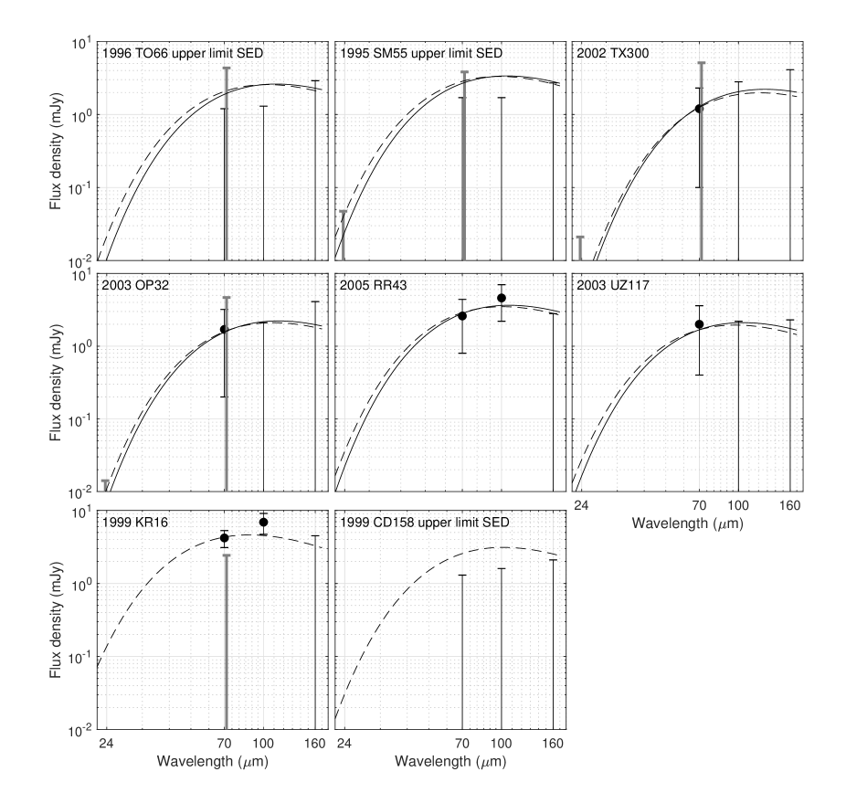
Figure 1: Modelled flux densities as function of wavelength calculated from solutions in Table 5. Solid lines (when present) are the preferred solutions, dashed lines are fixed beaming factor solutions with $\eta$=1.20, except for 2002 TX₃₀₀, where the solid line has $\eta$=1.8 and the dashed line $\eta$=0.73. Black data points are PACS data (70, 100 and $160\ \mathrm{\mu m}$) and grey points are from MIPS (23.68 and $71.42\ \mathrm{\mu m}$) normalized to the observing geometry of PACS. Error bars are 1$\sigma$ uncertainties or 1$\sigma$ upper limits. Upper limit solutions have been calculated for non-detected targets using the 2$\sigma$ flux density upper limit of the most limiting band (see text).

Table 5: Results of radiometric modelling. When different fixed beaming factors have been used, the preferred solution is given in bold.

Target	Instruments	No. of	$D$	$p_{\mathrm{V}}$	$\eta$	Solution	Bands included
		bands	(km)			type	in solution
Haumea	PACS, MIPS	7	2322x1704x	0.51$\pm$0.02	1.74${}_{-0.17}^{+0.18}$	fixed $D$, $p_{V}$	all PACS, MIPS-70
	SPIRE		1026				all SPIRE
1996 TO66	PACS, MIPS	4	$<$330	$>$0.20	1.74	fixed $\eta$	PACS-100
1996 TO66	PACS, MIPS	4	$<$290	$>$0.27	$1.20$	fixed $\eta$	PACS-100
1995 SM55	PACS, MIPS	5	$<$280	$>$0.36	1.74	fixed $\eta$	PACS-100
1995 SM55	PACS, MIPS	5	$<$250	$>$0.45	$1.20$	fixed $\eta$	PACS-100
2002 TX300	PACS, MIPS	5	323${}_{-37}^{+95}$	0.76${}_{-0.45}^{+0.18}$	1.8${}_{-0.9}^{+0.5}$	fixed $D$, $p_{V}$	PACS-70, PACS-100
2003 OP32	PACS, MIPS	5	274${}_{-25}^{+47}$	0.54${}_{-0.15}^{+0.11}$	1.74$\pm$0.17	fixed $\eta$	MIPS-24, PACS-70, PACS-100
2003 OP32	PACS, MIPS	5	248${}_{-23}^{+32}$	0.66${}_{-0.14}^{+0.15}$	$1.20\pm 0.35$	fixed $\eta$	MIPS-24, PACS-70, PACS-100
2005 RR43	PACS	3	300${}_{-34}^{+43}$	0.44${}_{-0.10}^{+0.12}$	1.74 $\pm$ 0.17	fixed $\eta$	all PACS
2005 RR43	PACS	3	268${}_{-26}^{+42}$	0.55${}_{-0.15}^{+0.13}$	$1.20\pm 0.35$	fixed $\eta$	all PACS
2003 UZ117	PACS	3	222${}_{-42}^{+57}$	0.29${}_{-0.11}^{+0.16}$	1.74 $\pm$ 0.17	fixed $\eta$	PACS-70, PACS-100
2003 UZ117	PACS	3	192${}_{-28}^{+54}$	0.39${}_{-0.15}^{+0.16}$	$1.20\pm 0.35$	fixed $\eta$	PACS-70, PACS-100
1999 KR16	PACS, MIPS	4	232${}_{-36}^{+34}$	0.105${}_{-0.027}^{+0.049}$	1.20 $\pm$ 0.35	fixed $\eta$	MIPS-70, all PACS
1999 CD158	PACS	3	$<$310	$>$0.13	1.20 $\pm$ 0.35	fixed $\eta$	PACS-70

(1) Size and geometric albedo from Ortiz et al. (2017); (2) Diameter from re-analysis of the occultation result of Elliot et al. (2010) (see text).

3.2 Haumea

The optical light curve of Haumea has a large amplitude (Rabinowitz et al. 2006), which is indicative of a shape effect. Time-resolved photometry shows a lower-albedo region on its surface, which may cover more than 20% of the instantaneous projected surface area (Lacerda et al. 2008). Lockwood et al. (2014) observed the optical light curve by Hubble and were able to resolve the contribution of the primary component excluding the contribution of Haumea’s moons. They report a light curve amplitude of 0.320$\pm$0.006 mag (valley-to-peak). Using this light curve Lockwood et al. (2014) derived Haumea’s size assuming hydrostatic equilibrium, an equator-on viewing geometry, and Hapke’s reflectance model (with parameters derived for the icy moon Ariel): $a=960$ km, $b=770$ km, and $c=495$ km for the semi-axes, respectively. Most recently, the shape of Haumea was derived in a more direct way from a stellar occultation (Ortiz et al. 2017): $a$=1161$\pm$30 km, $b$=852$\pm$4 km, $c$=513$\pm$16 km. Furthermore, the new density estimate based on this occultation result indicates that the assumption of hydrostatic equilibrium does not apply in the case of Haumea (Ortiz et al. 2017). The equivalent mean diameter of the projected surface corresponding to the above mentioned ellipsoid is $2a^{1/4}b^{1/4}c^{1/2}$= 1429$\pm$22 km, which is within the uncertainty of the less accurate radiometric spherical-shape size estimate of 1324$\pm$167 km (Lellouch et al. 2010). However, a size estimate done by a similar method but using more data points in far-infrared wavelengths gave a significantly smaller size of $1240_{-58}^{+69}$ km (Fornasier et al. 2013). The geometric albedo of Haumea based on the occultation is $p_{V}=0.51\pm 0.02$ (Ortiz et al. 2017). Since the calculation of the geometric albedo requires the absolute magnitude $H_{V}$ , Ortiz et al. (2017) used an updated value of $H_{V}$ for the time of the occultation and assumed a brightness contribution of 11% from the two moons and 2.5% from the ring.

In our further analysis we will use Haumea’s beaming factor. It has different values reported in the literature: (i) 1.38$\pm$0.71 (Lellouch et al. 2010) based on averaged PACS light curve data combined with a Spitzer observation using a NEATM-type radiometric model, (ii) 0.95${}_{-0.26}^{+0.33}$ (Fornasier et al. 2013) based on a NEATM-type model and averaged data from Herschel/PACS as well as observations from Herschel/SPIRE and Spitzer/MIPS covering a wavelength range from 70 to 350 $\mu m$, and (iii) $\eta=0.89_{-0.07}^{+0.08}$ based on the Lockwood et al. (2014) shape mentioned above and Spitzer/MIPS 70 $\mu m$ light curve using another thermal model with isothermal temperature at each latitude (as applied by Stansberry et al. 2008) as Haumea is rotating relatively quickly. Because of differences in the radiometric models applied, caution should be taken when comparing the beaming factor of Lockwood et al. (2014) with the other beaming factors. Lellouch et al. (2010) modelled also the PACS light curve of Haumea and determined the beaming factor depending on the assumed pole orientation such that $\eta$=1.15 if Haumea is equator-on and $\eta$=1.35 if the equator is at an angle of 15^∘.

In this work, we have determined the beaming factor $\eta$ by fixing the semi-axis and geometric albedo using the occultation result and then applying an “ellipsoidal-NEATM” with zero sun-target-observer phase angle (Brown 1985) and far-infrared fluxes of Fornasier et al. (2013) with minor updates. Since the measured fluxes have been obtained by averaging a light curve or by combining at least two separate observations taken several hours apart, we use an average projected size at a rotation of 45$\degr$ (in a coordinate system where rotation=0$\degr$ means that the longest axis is towards the observer). A one-parameter fit with the ellipsoidal thermal model gives $\eta$=1.74${}_{-0.17}^{+0.18}$. This beaming factor is higher than previous estimates when the accurate size was not available. While Haumea’s beaming factor is not unusual for objects at $\sim$50 AU distance from the Sun, there is an observational result that other high-albedo objects ($p_{V}>$0.20, see Fig. 2 in Lellouch et al. 2013) have lower beaming factors with the exception of Makemake, whose beaming factor is $\eta=2.29_{-0.40}^{+0.46}$ (Lellouch et al. 2013) based on Herschel/SPIRE data and fixed size and geometric albedo ($p_{V}\approx 0.77$) from a stellar occultation (Ortiz et al. 2012a). A fast rotation tends to increase the beaming factor $\eta$ but there are also other effects affecting $\eta$ such as increasing surface porosity, which lowers its value (Spencer et al. 1989). With $P$=7.7 h (Thirouin et al. 2010) Makemake is a slower rotator than Haumea.

The beaming factor $\eta$ is related to the thermal parameter $\Theta$ of Spencer et al. (1989), which is the ratio of two characteristic timescales: the timescale of radiating heat from the subsurface and the diurnal timescale. Figure 5 in Lellouch et al. (2013) shows the beaming factor as a function of the thermal parameter for a spherical object with an instantaneous subsolar temperature of $T_{0}=50$ K, which is close to the $T_{0}$ of Haumea that can be calculated via our Eq. 3 by setting $\eta=1$. Furthermore, Fig. 4 of Lellouch et al. (2013) shows that the relation between the beaming factor and the thermal parameter does not depend on small differences in the value of $T_{0}$ if the thermal parameter is $\Theta\lesssim$10. However, there is a strong dependence on the aspect angle of the rotation axis and based on the occultation Haumea is seen close to equator-on (Ortiz et al. 2017). The beaming factor derived in this work for Haumea implies a thermal parameter $\Theta$ in the order of magnitude of $\sim$3 if there is no surface roughness and up to a factor of approximately two higher in case of high roughness. Thermal inertia $\Gamma$ is directly proportional to the thermal parameter (Spencer et al. 1989)

$$\Gamma=\Theta\frac{\epsilon\sigma T_{0}^{3}}{\sqrt{2\pi}}\sqrt{P},$$ (4)

where $P$ is the rotation period given in Table 3. This estimate gives a thermal inertia of $\Gamma\sim$1 $\mathrm{J}\mathrm{m}^{-2}\mathrm{K}^{-1}\mathrm{s}^{-\frac{1}{2}}$, which is compatible with the finding of Lellouch et al. (2013) that most high-albedo objects have very low thermal inertias. The value derived in this work is higher than the thermophysical modelling of Santos-Sanz et al. (2017), which indicates that Haumea’s thermal inertia is $<$0.5 $\mathrm{J}\mathrm{m}^{-2}\mathrm{K}^{-1}\mathrm{s}^{-\frac{1}{2}}$ and probably as low as $<$0.2 $\mathrm{J}\mathrm{m}^{-2}\mathrm{K}^{-1}\mathrm{s}^{-\frac{1}{2}}$. Santos-Sanz et al. (2017) used thermal light curves observed by Herschel as well as the shape model and geometric albedo estimate available before the results from the occultation were analysed. Sophisticated thermophysical modelling using the occultation size and shape as well as contributions from the moons, the ring, and a dark spot on Haumea is beyond this work and will be analysed separately (Müller et al., in prep.). The observational result of a lack of high beaming factors of high-albedo objects mentioned earlier is reflected also onto thermal inertias inferred from measured beaming factors and rotational periods: high values of thermal inertia are excluded for high-albedo objects (see Fig. 7 in Lellouch et al. 2013). In addition to Haumea, another moderate to high-albedo TNO that has a value of thermal inertia determined via thermophysical modelling is Orcus. Using Herschel observations its thermal inertia has been determined to be 0.4$<$$\Gamma$$<$2.0 $\mathrm{J}\mathrm{m}^{-2}\mathrm{K}^{-1}\mathrm{s}^{-\frac{1}{2}}$ (Lellouch et al. 2013). Orcus has a geometric albedo of $p_{V}\approx$0.23 and a beaming factor of $0.97_{-0.02}^{+0.05}$ (Fornasier et al. 2013). Haumea’s thermal inertia estimated in this work is compatible with the thermal inertia determined for Orcus although its beaming factor is lower than that of Haumea. With its light curve period of $\sim$10 h (Thirouin et al. 2010), Orcus is a much slower rotator than Haumea but this difference is not enough to explain the difference in beaming factors. Orcus is likely to have a surface with more roughness than that of Haumea.

3.3 Occultation target 2002 TX₃₀₀

Target 2002 TX₃₀₀ was observed both by Herschel and Spitzer, but only the PACS/70 $\mu$m band gives a weak detection while the other four bands give upper limits. Although Lellouch et al. (2013) reported a three-band detection (all having signal-to-noise ratio $<$3), after an updated data reduction the PACS 100 and 160 $\mu$m bands are now considered upper limits. The Spitzer observations of 2002 TX₃₀₀ were of very short duration (Table 2) compared to the Herschel observations. We have ignored the Spitzer and PACS/160 $\mu$m data because those upper limits do not constrain the solution. A floating-$\eta$ solution that would be compatible with the optical constraint (Eq. 2) is not possible in the physical range of the beaming factor: 0.6$\leq$$\eta$$\leq$2.65 (limits discussed in Mommert et al. 2012 and Lellouch et al. 2013). However, for this target there is an independent size estimate available from a stellar occultation event in 2009.

The observations of the occultation event of 2002 TX₃₀₀ by several stations resulted in two useful chords. The diameter assuming a circular fit is 286$\pm$10 km (Elliot et al. 2010). While the occultation technique may give very accurate sizes of TNOs, it should be noted that in the case of 2002 TX₃₀₀ the result is based on two chords as a reliable elliptical shape fit would require at least three chords. In addition, the mid-times of the occultations reported by the observing stations at Haleakala and Mauna Kea differ by 31.056 s (Table 1 in Elliot et al. 2010). Such an offset, if real, would be compatible with a hypothesis that the two chords are from two separate objects, that is, that 2002 TX₃₀₀ could be a binary. Elliot et al. (2010) mention that one of the chords had to be shifted by 32.95 s to get them aligned for a circular fit (fit parameters were radius, centre position in the sky plane relative to the occulted star, and timing offset). The two-chord occultation and a large timing uncertainty imply a larger uncertainty also in the adopted effective size estimate. The actual shape of an object the size of 2002 TX₃₀₀ may differ from a spherical one since self-gravity is not strong enough for an icy $\lesssim$400 km object to result in a sphere-like shape. The optical light curve is double-peaked which indicates a shape effect. If we assume a Maclaurin spheroid with a rotation period of 8.15 hours and a uniform density of 1.0 gcm^-3 , the axial ratio a/c would be 1.27 according to the figure of equilibrium formalism. This ratio is even larger for lower densities. An ellipsoidal fit with a/c$\sim$1.3 would give a major axis of 363 km, a minor axis of 289 km, and an effective diameter of 323 km, which is 13% more than the circular fit would give. Even larger effective diameters would result if one of the chords is moved arbitrarily within the timing shift.

The geometric albedo is calculated from the occultation size via absolute magnitude $H_{\mathrm{V}}$. In this work (see Table 3) we use $H_{\mathrm{V}}$=3.365$\pm$0.044 mag based on a phase curve study (Rabinowitz et al. 2008), which is different from the $H_{\mathrm{V}}$ used by Elliot et al. ($\approx$3.48). Using the Elliot et al. size for a circular fit and the Rabinowitz et al. absolute magnitude results in a very high geometric albedo of 0.98$\pm$0.08. This is higher than the geometric albedo of 0.88$\pm$0.06 reported by Elliot et al. (2010) for a circular fit but is within their extended error bar when uncertainty due to possible elliptical fits is taken into account. A geometric albedo of $p_{V}$=0.98 would be the highest value among TNOs and similar to that of the dwarf planet Eris (0.96${}_{-0.04}^{+0.09}$, Sicardy et al. 2011).

In this work we adopt the above mentioned elliptical solution based on a/c=1.3 and use 323 km as the effective diameter. The lower uncertainty limit is estimated as the difference of this size and the circular solution. The upper uncertainty limit is challenging to estimate from the occultation data alone. Here we use the fact that 2002 TX₃₀₀ is close to the detection limit of Herschel observations. If the PACS/70 $\mu$m data point is interpreted as an upper limit then using the 2$\sigma$ flux limit as explained in Sect. 3.1 and a conservative high beaming factor we get an upper limit of effective diameter: 418 km. Thus, our new size estimate for 2002 TX₃₀₀ is 323${}_{-37}^{+95}$ km and geometric albedo estimate $p_{V}$=0.76${}_{-0.45}^{+0.18}$. This geometric albedo is higher but within the large uncertainty compared to Haumea’s $p_{V}$=0.51$\pm$0.02 (Ortiz et al. 2017).

Using fixed estimates of diameter and geometric albedo in the thermal modelling we can fit the beaming factor. The same approach was used by Lellouch et al. (2013). The new size and geometric albedo estimates given above result in a beaming factor of $\eta$=1.8${}_{-0.9}^{+0.5}$. This is higher, but compatible within error bars, compared to an earlier result by Lellouch et al. (2013): $\eta$=1.15${}^{+0.55}_{-0.74}$, which is based on the smaller size and higher geometric albedo reported by Elliot et al. (2010) as well as on an earlier version of flux densities from Herschel. For comparison, using the same size estimate of Elliot et al. (2010) and geometric albedo of $p_{V}$=0.98 results in a beaming factor of $\eta$=0.73 using updated Herschel fluxes (see also Fig. 1).

3.4 Fixed-$\eta$ fits

Fixed-$\eta$ solutions were used when floating-$\eta$ fits failed. Most of the TNO literature has used the default value $\eta$=1.20$\pm$0.35 (Stansberry et al. 2008) based on a sample of TNOs of various dynamical classes observed by Spitzer where CKBOs were under-represented. Based on a sample of 13 CKBOs observed by Herschel and/or Spitzer, Vilenius et al. (2014) derived an average of $\eta$=1.45$\pm 0.46$. A larger sample of 85 objects observed by Herschel and Spitzer representing various dynamical classes gave a mean value of $\eta$=1.175$\pm$0.45 (Lellouch et al. 2017).

As mentioned in Sect. 3.1 the data quality did not allow a floating-$\eta$ solution for most targets. Only Haumea and 2002 TX₃₀₀ have a beaming factor determined but the latter was weakly detected only at one thermal band (see Table 1) and has large error bars, which cover most of the physically plausible range of beaming factor values. Since the beaming factor depends on surface properties and heliocentric distance (e.g. Lellouch et al. 2013), we do not have a reliable average $\eta$ for the Haumea family. In this work we adopt the value of Haumea from the one-parameter fit using the occultation size and albedo as explained in Sect. 3.2, but approximate the asymmetric uncertainties with a symmetric Gaussian distribution in further analysis: $\eta$=1.74$\pm$0.17. We have adopted this value in our fixed-$\eta$ fits for confirmed family members (2003 OP₃₂, 2005 RR₄₃, 2003 UZ₁₁₇, and upper limits of 1996 TO₆₆ and 1995 SM₅₅), but show also the results based on the canonical default value $\eta$=1.20$\pm$0.35 in Table 5. The rotational periods of 2003 OP₃₂, 2005 RR₄₃, and 2003 UZ₁₁₇ have been measured and we can estimate the value of their thermal parameters (Eq. 4) assuming a value for the thermal inertia. Plausible values are 1.0$<$$\Gamma$$<$3.0 $\mathrm{J}\mathrm{m}^{-2}\mathrm{K}^{-1}\mathrm{s}^{-\frac{1}{2}}$ if the thermal inertias of these three objects do not differ significantly from that of Haumea’s or the average thermal inertia (see Sect. 3.2). With this range of thermal inertia, the thermal parameter is 2.2$<\Theta<$8.4 for the three objects. Therefore, a beaming factor value of $\eta\approx 1.74$ is possible for these three objects. We continue to use the default value of the beaming factor 1.20$\pm$0.35 for the two moderate-albedo probable dynamical interlopers (1999 KR₁₆ and 1999 CD₁₅₈) modelled in this work, as the probable dynamical interlopers are in a different cluster in a colour-albedo diagram (see Fig. 2 in Lacerda et al. 2014a) and thus probably do not share the surface properties of Haumea family members.

3.5 Comparison with earlier results

Four of the family members, in addition to Haumea, have been observed by Spitzer. Based on upper limits at two Spitzer/MIPS bands, Brucker et al. (2009) reported 1$\sigma$ limits for 2002 TX₃₀₀ as $D$$<$210 km and $p_{V}$$>$0.41. As discussed in Sect. 3.3 the size of this object, based on a stellar occultation, is larger (Table 5) than the 1$\sigma$ upper limit by Spitzer. The other family members do not have published Spitzer results (except Haumea). Altenhof et al. (2004) observed 1996 TO₆₆ and 1995 SM₅₅ with the 30 m telescope of the Institute for Radio Astronomy in the Millimeter Range (IRAM) at 1.2 mm wavelength. The non-detections gave limits (Grundy et al. 2005) 1996 TO₆₆: $D$$<$$902$ km, $p_{R}$$>$0.033 and 1995 SM₅₅: $D$$<$704 km, $p_{R}$$>$0.067. The results of this work give more constraining limits: both targets are smaller than previous limits and have moderate to high albedos (Table 5).

Herschel results of the probable dynamical interloper 1999 KR₁₆ have been published by Santos-Sanz et al. (2012). After significant flux updates at 100 and 160 $\mu m$ (see Sect. 2.1) as well as a fainter $H_{V}$, the size estimate is 9% smaller (232${}_{-36}^{+34}$ km compared to the previous 254$\pm$37 km) but the two results are within each others uncertainties. Geometric albedo is now slightly lower ($p_{V}$$=$0.105${}_{-0.027}^{+0.049}$) than in Santos-Sanz et al. ($p_{R}$=0.204${}_{-0.050}^{+0.070}$, which corresponds to a V-band albedo of $p_{V}$$\approx$0.14 using the V-R colour from Table 4).

4 Sample results and discussion

Table 6: Diameters and albedos of confirmed Haumea family members.

Name	$\Delta v_{\mathrm{min}}$	H2O	Thermal	Diameter	Geometric	Size/albedo
	(m s-1)	reference	data	(km)	albedo	reference
136108 Haumea (2003 EL61)	323.5	Brown et al. (2007)	(S+H)	2322x1704	0.51$\pm$0.02	O17
				x1026
Hi’iaka	…	Barkume et al. (2006)	…	383${}_{-113}^{+74}$ (*)	default	TW
Namaka	…	Fraser & Brown (2009)	…	193${}_{-65}^{+48}$ (*)	default	TW
19308 (1996 TO66)	24.2	Brown et al. (1999)	(S+H)	210${}_{-62}^{+40}$ (*)	default	TW
24835 (1995 SM55)	149.7	Brown et al. (2007)	(S+H)	243${}_{-71}^{+46}$ (*)	default	TW
55636 (2002 TX300)	107.5	Licandro et al. (2006)	S+H	$323_{-37}^{+95}$	$0.76_{-0.45}^{+0.18}$	TW, E10
86047 (1999 OY3)	292.8	Ragozzine & Brown (2007)	…	91${}_{-27}^{+17}$ (*)	default	TW
120178 (2003 OP32)	123.3	Brown et al. (2007)	S+H	274${}_{-25}^{+47}$	0.54${}_{-0.15}^{+0.11}$	TW
145453 (2005 RR43)	111.2	Brown et al. (2007)	H	300${}_{-34}^{+43}$	0.44${}_{-0.10}^{+0.12}$	TW
308193 (2005 CB79)	96.7	Schaller & Brown (2008)	…	224${}_{-48}^{+37}$ (*)	default	TW
386723 (2009 YE7)	85	Trujillo et al. (2011)	…	226${}_{-50}^{+40}$ (*)	default	TW
2003 SQ317	148.0	Snodgrass et al. (2010)	…	98${}_{-24}^{+20}$ (*)	default	TW
2003 UZ117	66.8	Schaller & Brown (2008)	H	222${}_{-42}^{+57}$	0.29${}_{-0.11}^{+0.16}$	TW

Table 7: Candidate Haumea family members (membership neither confirmed nor rejected).

Target	$\Delta v_{\mathrm{min}}$	Class
	(m s-1)
1998 HL151	142.5	CKBO
1999 OK4	161.5	CKBO
2003 HA57	214.3	Plutino
1997 RX9	306.1	CKBO
2003 HX56	363.2	CKBO
2003 QX91	222.0	Res 7:4
130391 (2000 JG81)	235.1	Res 2:1
315530 (2008 AP129)	107$\pm$2	CKBO
2014 FT71	30$\pm$1	CKBO

Thirty-five TNOs were identified by Ragozzine & Brown (2007) as potential Haumea family members based on their orbital dynamics and velocities with respect to the centre of mass of the collision, which is approximated by the orbit of Haumea before diffusion under the influence of the 12:7 mean-motion resonance with Neptune. Tables 10 and 12 give the albedos and diameters of the Haumea family members and of probable dynamical interlopers that have measurements relevant to assessing their membership in the family. Table 11 summarizes ejection velocities for dynamically similar TNOs that lack any such data, and so are candidates for membership. The ejection velocities in Tables 10 and 11 may be systematically uncertain for the ensemble of objects, but do reflect the rank order, from slowest to largest ejection velocity (Ragozzine & Brown 2007).

The ejection velocities of 2008 AP₁₂₉, 2009 YE₇, and 2014 FT₇₁ have been calculated by simulations in this work. These results are based on 50 Myr-averaged orbital elements for both the observed orbits and the orbits of test particles in simulated clouds. We considered the nominal orbit plus two orbits with $3\sigma$ uncertainties in a-e space and required the clouds of test particles to cover the three orbits in order to determine the minimum ejection velocity of the cloud of test particles. In the case of 2014 FT₇₁ the nominal orbit and one other orbit have been influenced by the 7:4 mean motion resonance with Neptune, whereas one orbit is not influenced by this resonance and resulted in a significantly higher ejection velocity of 178$\pm$2 m/s than our preferred result of 30$\pm$1 m/s.

Table 8: Diameters and geometric albedos of probable dynamical interlopers of the Haumea family.

Name	Diameter	Geometric	Ref.	Cause of
	(km)	albedo		exclusion
1996 TR66	…	…		NIR colors
1999 KR16	232${}_{-36}^{+34}$	0.105${}_{-0.027}^{+0.049}$	(1)	Very red
2002 AW197	$768_{-38}^{+39}$	$0.112_{-0.011}^{+0.012}$	(3)	NIR spectra
1999 RY215	$263_{-37}^{+29}$	$0.0325_{-0.0065}^{+0.0122}$	(3)	(J-HS) color
Salacia	$901\pm 45$	0.044$\pm$0.004	(4)	NIR spectra
Makemake	1430$\pm$9	0.77$\pm$0.03	(2)	Methane ice
1998 WT31	…	…		Red slope
2005 UQ513	$498_{-75}^{+63}$	$0.202_{-0.049}^{+0.084}$	(3)	Red slope
1996 RQ20	…	…		Very red
1999 CD158	$<$310	$>$0.13	(1)	Very red
1999 OH4	…	…		NIR colors
2000 CG105	…	…		NIR colors
2001 FU172	…	…		Red slope
2001 QC298	$303_{-32}^{+29}$	$0.063_{-0.018}^{+0.029}$	(3)	(J-HS) color
2002 GH32	$<$230	$>$ 0.13	(3)	Very red
2003 TH58	…	…		(J-HS) color
2004 PT107	$400_{-51}^{+45}$	$0.033_{-0.007}^{+0.011}$	(3)	(J-HS) color
2005 GE187	…	…		(J-HS) color
2010 KZ39	…	…		NIR colors

4.1 Size and albedo distributions

We have constructed a combined probability density distribution of geometric albedos based on the few measured targets. The asymmetric uncertainties have been taken into account using the approach of Mommert (2013). Instead of having two tails from a normal distribution, which would create a discontinuity in case of asymmetric error bars, we use a log-normal distribution. The combined geometric albedos (Fig. 2) of four Haumea family members that have measured geometric albedos (from Table 5) have a median of $p_{V}$=0.48${}_{-0.18}^{+0.28}$ using the fixed-$\eta$ solutions based on Haumea’s beaming factor for 2003 OP₃₂, 2005 RR₄₃, and 2003 UZ₁₁₇ (the geometric albedo of 2002 TX₃₀₀ is derived from a stellar occultation) and $p_{V}$=0.58${}_{-0.21}^{+0.27}$ if the canonical beaming factor is used instead.

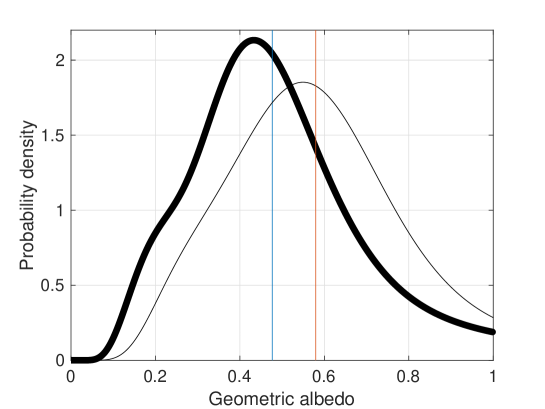
Figure 2: Combined probability density distribution of geometric albedos of confirmed Haumea family members 2002 TX₃₀₀, 2003 OP₃₂, 2005 RR₄₃, and 2003 UZ₁₁₇. The thick line is the albedo distribution assuming the solutions based on the beaming factor value $\eta$=1.74$\pm$0.17 for 2003 OP₃₂, 2005 RR₄₃, and 2003 UZ₁₁₇ and the thin line assuming the solutions with the canonical beaming factor value $\eta$=1.20$\pm$0.35. The median values of the two distributions are $p_{V}=0.48_{-0.18}^{+0.28}$ (blue vertical line indicates the median) for the preferred solutions and $p_{V}=0.58_{-0.21}^{+0.27}$ (red vertical line) assuming the canonical beaming factor.

We have measured sizes for four confirmed family members (other than Haumea). For the other family members absolute visual magnitudes are available. The size distribution of the Haumea family, excluding Haumea (Fig. 3), is constructed in a statistical way by using measured size values when available and otherwise by assigning an albedo from the distribution shown in Fig. 2 and using the absolute visual magnitudes $H_{V}$ (Table 4). Size distributions are formed 50000 times so that each measured or inferred size may vary according to its error bar. The slope parameter in the size range 175-300 km is $q=$3.2${}_{-0.4}^{+0.7}$. All the measured effective diameters are $>150$ km and the decrease of the slope below this size may be due to an incomplete sample in the size bins $<150$ km (see the lower panel of Fig. 3) as only two confirmed family members (see Table 10) have size estimates $<100$ km based on the assumed albedo. If instead of using the sizes and albedo distribution based on the fixed-$\eta$ value of 1.74 we use solutions based on the canonical value of 1.20 (see Table 5 and Fig. 2), then the slope is steeper $q$=3.8${}_{-0.5}^{+0.9}$ although it is within the uncertainties of the preferred solution. However, sizes are generally smaller and geometric albedos higher when the canonical beaming factor has been used and there are less simulated objects in the 300 km size bin. Considering the size range 150-275 km (i.e. excluding the last size bin) gives a result that is similar to the nominal solution: $q=$3.1${}_{-0.4}^{+0.7}$.

The slope of the size distribution obtained here can be compared with the slope of dynamically hot CKBOs since most of the family members and probable dynamical interlopers belong to that class. The large end of the size distribution of dynamically hot CKBOs is $q=$4.3$\pm$0.9 (Vilenius et al. 2014) turning into a shallower slope of $q=2.3\pm$0.1 in the size range 100-500 km. We have also determined the size distribution of $<$500 km probable dynamical interlopers from Table 12 (using average geometric albedo of dynamically hot CKBOs from Vilenius et al. (2014) and $H_{V}$ from MPC when no measured size available): q=2.0$\pm$0.6, which is compatible with the slope parameter of the general hot CKBO population. Comparing the two above-mentioned slope parameters to those determined for the Haumea family ($q\sim 3$) indicates that the family has a slope that is steeper than the background population of dynamically hot CKBOs in the same size range.

There are different models for the slope of the size distributions of collisional fragments in the literature. The value determined in this work is approximately compatible with the classical slope of -2.5 (Dohnanyi 1969; Carry et al. 2012), which corresponds to $q=3.5$ in our definition of the slope parameter.

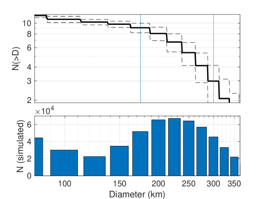
Figure 3: Combined statistical distribution of sizes (measured if available, otherwise inferred from the albedo distribution and $H_{V}$) of confirmed Haumea family members, including the moons. The bin size is 25 km. The size range 150–300 km for which the slope parameter is determined is indicated by the blue and red vertical lines. The lower panel shows the size histogram of 50000 randomly generated objects (see text).

4.2 Albedo and family membership

The albedos and diameters of the TNOs assumed to be dynamical interlopers in the Haumea family are given in Table 12. The table also briefly summarizes the rationale for excluding each object from inclusion as a true member of the collisional family. The albedo values are an independent data set that bears on the question of family membership. Excluding Makemake and Salacia, each of comparable size to Haumea and therefore inconsistent with the assumption that Haumea itself defines the centre of mass for the collisional family, the median geometric albedo for these objects is 0.08${}_{-0.05}^{+0.07}$. Most of the objects in Table 12 are dynamically hot CKBOs, and their average albedo is consistent with the average albedo of those objects, $p_{V}$ = 0.085${}_{-0.045}^{+0.084}$ (Vilenius et al. 2014). As discussed in Sect. 4.1, the average albedo measured for the four accepted family members is 0.48, much higher than for the objects in Table 12. This suggests that these objects do not have albedos similar to those of the accepted family members (although the sample sizes, six interlopers and four family members, are very small). Of the objects in Table 12, only the hot CKBO 2005 UQ₅₁₃ has an unusually high albedo, and its albedo is significantly higher than the average for hot CKBOs in general. Our results for 1999 CD₁₅₈ and 2002 GH₃₂ suggest that they may also have high albedos. Table 12 gives the 2$\sigma$ lower limits on albedo and upper limits on size (i.e. the probability that the geometric albedo is $<$0.13 is $\approx$4.6%). In summary, albedo measurements for objects previously identified as dynamical interlopers seem to support that identification in general, but suggest that three of them may have unusually high albedos, and further investigation may be warranted. It is unfortunate that there is not more data constraining the albedos and diameters of both the interlopers and the family members.

The Haumea family members have significantly higher albedos than the averages of scattered disk, detached, or cold CKBOs, which are the dynamical classes with the highest average albedos (Santos-Sanz et al. 2012; Vilenius et al. 2014). For mid-sized TNOs, such as Haumea family members, the high albedo surface indicates lack of hydrocarbons, which would have produced a darker and redder surface over long periods of exposure to space weathering (Brown 2012). This is compatible with the collisional hypothesis, which states that the fragments are high-albedo water ice pieces from the mantle of proto-Haumea. In a colour-albedo plot the Haumea family members, with their high albedos, are distinct from the probable dynamical interlopers, which are more widely spread in the colour-albedo plot of Lacerda et al. (2014a, Fig. 2).

4.3 Mass and ejection velocity

The masses of Haumea’s moons Hi’iaka and Namaka are (20.0$\pm$1.2)$\times 10^{18}$ kg and (2.0$\pm$1.6)$\times 10^{18}$ kg (Ragozzine & Brown 2009; Ćuk et al. 2013). For the other family members we estimate masses assuming bulk densities of 1 g cm^-3. The confirmed members would constitute approximately 2.4% of the mass of Haumea (using sizes from Table 10 when no mass or size measurement available). The largest family member, the moon Hi’iaka, would alone constitute 21% of the mass of the family excluding Haumea and the five largest family members would be more than half of the total mass of the family (excluding Haumea). Using the alternative radiometric solutions of Table 5 and the lower median geometric albedo results in a mass estimate of 2.0%. If all the candidate family members in Table 11 were be confirmed, they would constitute $\sim$0.2% of Haumea’s mass.

The scenarios in which the proto-moon of Haumea underwent fission to produce a family presented by Ortiz et al. (2012b) require that the mass of the moons and the family members is less than 20% of Haumea’s mass. Ortiz et al. (2012b) had only one measured albedo available (2002 TX₃₀₀) and they used a default geometric albedo of 0.6 for other family members. Our new observations give more confirmation in using a high albedo and our new mass estimate of the family is compatible with the mass ratio assumption used by Ortiz et al. (2012b). Our mass estimate of 2.4% does not exclude the formation mechanisms by disruption of a large satellite of proto-Haumea (Schlichting & Sari 2009), which predicts an upper mass ratio limit of 5%. The mechanism proposed by Leinhardt et al. (2010), where two equal-sized objects merge, predicts a mass ratio of 4-7% (Volk & Malhotra 2012), which is higher than our current estimate.

The ejection velocity of a fragment and its mass are related via a power law. Assuming a constant density for all family members, this relation may be written in terms of the diameter as (Lykawka et al. 2012) $v_{e}\propto D^{-\gamma}$, where $v_{e}$ is the ejection velocity and the power-law slope $\gamma$ is $\lesssim$ 0.5 (Zappala et al. 2002). Figure 4 shows a fit to effective diameters and velocities from Table 10. A fit using confirmed family members gives $\gamma$=0.62, which is slightly larger than the upper limit of plausible values. Lykawka et al. (2012) and references cited therein note that there is often large scatter in the ejection velocity values and large ratios of maximum-to-minimum values. Therefore, another fit is made by ignoring the minimum and maximum velocities (1996 TO₆₆ and 1999 OY₃). This gives a lower value of $\gamma$=0.21. We have repeated the fit with an extended data set including all the candidate family members (Table 11 and inferred sizes using the geometric albedo distribution of the Haumea family). The extended data set gives $\gamma$=0.61 for all data and $\gamma$=0.50 when minimum and maximum velocities are excluded (1996 TO₆₆ and 2003 HX₅₆). In the above calculations we used absolute visual magnitudes and an assumed geometric albedo of $p_{V}$=0.48 to assign diameters to objects lacking a measured size. If the canonical value of the beaming factor is used in fixed-$\eta$ solutions of the family members, the resulting median geometric albedo is higher: $p_{V}$=0.58. With this geometric albedo the result (confirmed and candidate family members excluding minimum and maximum velocities) is $\gamma$=0.46, which indicates that the result is not sensitive to a moderate difference in the assumed geometric albedo.

The fitted values indicate that ejection velocities are dependent on diameter although in some of the cases the power-law slope is 0.5-0.6, which is higher than expected from theory. This means that smaller fragments of the Haumea family have been dispersed in the orbital element space much more than the currently known larger fragments (Lykawka et al. 2012). This may affect theories of the formation of the family that try to solve the problem of too low velocities: an average based on those velocities is probably biased by the fact that we have only observed, and discovered, the largest fragments of the family, which have lower velocities than smaller fragments.

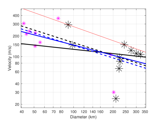
Figure 4: Distribution of ejection velocities. The large black dots are confirmed Haumea family members (Table 10) and the magenta dots are candidate family members (Table 11). The dashed black line is a fit to all confirmed family members ($\gamma$=0.62); the solid black line is a fit to the same data but excluding the minimum and maximum velocities ($\gamma$=0.21). The red line is a limiting case of the confirmed family members ($\gamma=0.68$). The dashed blue line is a fit to all confirmed and candidate family members ($\gamma$=0.61) and the solid blue line a fit to the same data excluding minimum and maximum velocities ($\gamma=0.50$).

4.4 Correlations

The small number of reliably measured Haumea family members and dynamical interlopers makes it challenging to detect correlations. The diameter and geometric albedo results (Table 5) suggest a positive correlation but, when taking into account the error bars (Peixinho et al. 2015), for the Haumea family objects we obtain a Spearman correlation coefficient of $\rho_{\,D\,p_{V}}=0.65^{+0.22}_{-0.45}$ with a P-value of 0.40 (i.e. confidence level CL$=0.84\,\sigma$), being, therefore, not significant. For the eight dynamical interlopers (Table 12) the correlation strength appears weaker, but the evidence is of the same order as in the Haumea family members and also not significant: $\rho_{\,D\,p_{V}}=0.37^{+0.38}_{-0.54}$ (P-value$=0.38$; CL$=0.88\,\sigma$).

Nevertheless, some remarks about minimum sampling for detections can be made. Supposing that the correlation between effective diameters and geometric albedos among the Haumea family was $\rho=0.9$, given our error bars and the low dispersion of albedos and diameters, such a correlation would be observationally “degraded” to $\sim 0.65$ (see Peixinho et al. 2015) and we would need a sample of $n\geq 39$ objects to have a risk lower than $10\%$ of missing it, if we aim at a $3\sigma$ level detection. Analogously, regarding the dynamical interlopers, even if their true diameter-albedo correlation was $\rho=0.4$, we would need a sample of $n\geq 112$ objects to ensure the detection. Most of the dynamical interlopers are classified as dynamically hot CKBOs and a sample of 26 objects in that class (excluding Haumea family and dwarf planets) showed no evidence of a diameter-albedo correlation at 3$\sigma$ level taking into account the error bars (Vilenius et al. 2014).

To confirm that the diameter-albedo correlation among the Haumea family objects would indeed be different from the one among the dynamical interlopers, at a $3\sigma$ level, we would need to increase the sampling required to detect the presence of the correlations by a factor of $2.5$ compared to the numbers of objects given above. The accuracy of size and albedo estimates can improve in the future, for example by more stellar occultations. If the error bars were lower than $\sim 5\%$, then a sample of 15 Haumea family objects and 112 dynamical interlopers would be enough to confirm a difference between $\rho$=0.9 and $\rho$=0.4 at a 3$\sigma$ level.

5 Conclusions

We have measured the sizes and geometric albedos of three confirmed Haumea family members: 2003 OP₃₂, 2005 RR₄₃, and 2003 UZ₁₁₇. In addition, we have updated the results of 2002 TX₃₀₀, 1996 TO₆₆, 1995 SM₅₅, and 1999 KR₁₆. We have also refined or determined optical phase coefficients for several family members and candidate members and have determined the ejection velocities of 2008 AP₁₂₉, 2009 YE₇, and 2014 FT₇₁. The ejection velocity is inversely correlated with the fragment diameter, and therefore the Haumea family may be less compact than thought. An average ejection velocity is probably biased by the fact that we have only observed, and discovered, the largest fragments of the family, which have lower velocities than smaller fragments.

Our analysis has utilized the results of the stellar occultation by Haumea (Ortiz et al. 2017) and has the following main conclusions:

1. Our measurements indicate that Haumea family members have a diversity of high to very high albedos and the lowest albedo among the detected objects is $\sim$0.29 and the albedo limit of non-detected targets is $\sog$0.2, which is higher than the average albedo of TNOs ($\sim$0.10). The median albedo of the Haumea family is $p_{V}$=0.48${}_{-0.18}^{+0.28}$. The highest-albedo member is 2002 TX₃₀₀.

2. The median geometric albedo of probable dynamical interlopers in the Haumea family is 0.08${}_{-0.05}^{+0.07}$, consistent with that of the dynamically hot CKBO population, and much lower than that for the accepted family members. Object 2005 UQ₅₁₃ does have an unusually high albedo (0.22), and two other objects (1999 CD₁₅₈ and 2002 GH₃₂) have 2$\sigma$ lower limits on their albedos of 0.13. Many Haumea family members and dynamical relatives lack albedo determinations, making interpretation of these albedo results tentative, but there is no strong evidence based on albedo that any of the dynamical interlopers should be considered as possible family members.

3. Using measured sizes when available and an average albedo with optical absolute brightness for other family members, we determine the cumulative size distribution and find its slope to be $q$=3.2${}_{-0.4}^{+0.7}$ for diameters 175$<$D$<$300 km. This is steeper than the slope of dynamically hot CKBOs in general in the same size range.

4. We estimate the confirmed family members and the two moons to constitute 2.4% of the mass of Haumea.

5. The ejection velocity depends on diameters of the fragments with a power-law slope of 0.21 (ignoring the minimum and maximum velocities). If candidate family members are included, to cover a broader diameter range, the slope is steeper: 0.50.

6. We have determined Haumea’s beaming factor: $\eta$$=$$1.74_{-0.17}^{+0.18}$, which indicates a thermal inertia of $\Gamma$$\sim$1 $\mathrm{J}\mathrm{m}^{-2}\mathrm{K}^{-1}\mathrm{s}^{-\frac{1}{2}}$.