The INTERNODES method for the treatment of non-conforming multipatch geometries in Isogeometric Analysis

Abstract

In this paper we apply the INTERNODES method to solve second order elliptic problems discretized by Isogeometric Analysis methods on non-conforming multiple patches in 2D and 3D geometries. INTERNODES is an interpolation-based method that, on each interface of the configuration, exploits two independent interpolation operators to enforce the continuity of the traces and of the normal derivatives. INTERNODES easily handles both parametric and geometric NURBS non-conformity. We specify how to set up the interpolation matrices on non-conforming interfaces, how to enforce the continuity of the normal derivatives and we give special attention to implementation aspects. The numerical results show that INTERNODES exhibits optimal convergence rate with respect to the mesh size of the NURBS spaces an that it is robust with respect to jumping coefficients.

Key words. Isogeometric Analysis, Multipatch Geometries, Domain Decomposition Methods, Non-conforming Interfaces, Internodes, Elliptic Problems

1 Introduction

Nowadays Isogeometric Analysis (IgA) [9] represents one of the most popular methods for numerical simulations. Its paradigm consists in expanding the Partial Differential Equations (PDE) solution with respect to the basis functions of the same type of the ones (either B-splines or NURBS) used to describe the geometry of the computational domain generated by CAD software.

Often, real-life problems are defined on complex geometries that usually consist of several patches. Moreover these patches can feature non-conformity.

By non-conformity we mean either geometrical non-conformity or parametric non-conformity. The former one occurs when two adjacent patches share a common boundary in the physical space only approximately (e.g., as result of CAD modeling operation) and we say that the interfaces are non-watertight; an example is shown in Fig. 1 (a).

In the case that two interfaces are watertight, however we can face parametric non-conformity that means that different and totally unrelated discretizations (not necessarily the refinement one of the other) are considered inside the patches sharing the same interface (or only a part of it); two examples are given in Fig. 1 (b) and (c).

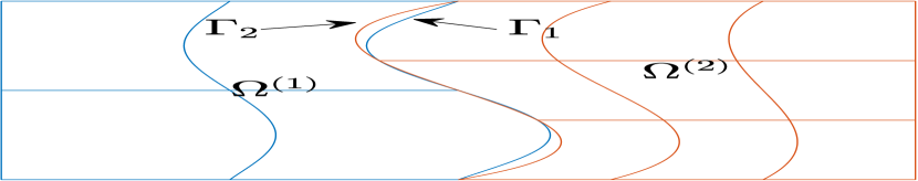
(a)

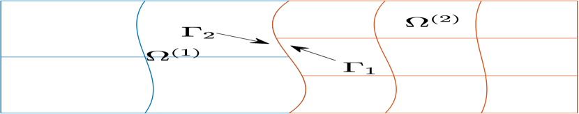
(b)

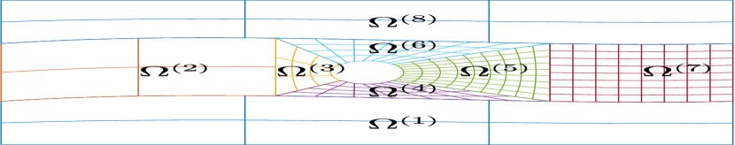
(c)

Figure 1: Non-conforming patches: (a) non-watertight patches, geometric non-conformity; (b) and (c) watertight patches but non-matching parametrizations at the interface

In the last years, the treatment of multipatch geometries has been investigated in several papers, far from be exhaustive we mention [10, 11, 26, 37, 41, 47, 8, 7, 34, 30, 27, 43, 6, 32, 15, 29]. In this paper we propose to apply the INTERNODES method to solve elliptic problems within the IgA framework on non-overlapping and non-conforming multipatch configurations.

Overlapping multi-patch domains without trimming have been faced in the Isogeometric Analysis context in [29]. In this very recent paper the authors propose the Overlapping Multi-Patch method, which is a non-iterative reformulation of the Schwarz method (see, e.g. [44, 40]).

INTERNODES (INTERpolation for NOnconforming DEcompositionS) [17, 21] is a general purpose method to deal with non-conforming discretizations of PDEs in 2D and 3D geometries split into non-overlapping subdomains (in fact IgA patches play the role of non-overlapping subdomains in the domain decomposition context [44, 40]). The method was proposed in [17] to solve elliptic PDEs by Finite Element Methods (FEM) and Spectral Element Methods (SEM) on two non-conforming subdomains, then its theoretical analysis, as well as its extension to decompositions with more than two subdomains, has been carried out in [21, 22, 24].

INTERNODES has been successfully applied to solve Navier-Stokes equations ([19, 20]) and multi-physics problems like the Stokes-Darcy coupling to simulate the filtration of fluid in porous domains [23, 24] and the Fluid-Structure Interaction problem [19, 20].

It has been proved that, inside the FEM-SEM context, INTERNODES exhibits optimal accuracy with respect to the $H^{1}$-broken norm, i.e., the error between the global INTERNODES solution and the exact one is proportional to the best approximation error inside the subdomains.

Inside the subregions (or patches) of the decomposition we discretize the PDE (here we have implemented the Galerkin formulation of IgA) by using NURBS spaces that are totally unrelated one each other.

To enforce the continuity of the traces and the equilibration of the fluxes across the interfaces between two adjacent patches, INTERNODES exploits two independent interpolation operators: one for transferring the Dirichlet trace of the solution, the other for the normal derivatives. Like mortar methods, INTERNODES tags the opposite sides of an interface either master or slave: the continuity of the traces is enforced on the slave side of the interface (more precisely the Dirichlet trace is interpolated from the master side to the slave one), while the equilibration of the fluxes is enforced on the master side of the same interface (the normal derivative is interpolated in a suitable way from the slave side to the master one).

In this paper we apply the interpolation at the Greville abscissae of the knot vectors [38, 16, 1], nevertheless other choices are possible (see, e.g. [1, 35]).

One of the strength of INTERNODES just consists in working with totally unrelated discretization spaces (with different sets of control points and weights and different basis functions) without the need to enrich the NURBS spaces or to insert necessary knots (as, e.g. T-splines do) to ensure full compatibility at the interfaces.

When two interfaces are watertight (as in Fig. 1 (b) and (c)) the point inversion from one interface to the adjacent one is well defined also for non-matching parametrizations and standard NURBS interpolation is exploited to implement INTERNODES. When instead the interfaces are non-watertight (as in Fig. 1 (a)) we overcome the difficulty to project the Greville abscissae from one face to the non-watertight corresponding one, by exploiting the Radial Basis Functions interpolation (see, e.g., [18, 19] in the FEM context and [34] in the IgA context).

To interpolate correctly the normal derivatives we need to assemble local interface mass matrices, but differently than in mortar methods, no cross-mass matrix involving basis functions living on the two opposite sides of the interface and no ad hoc numerical quadrature ([5]) are required by INTERNODES to build the inter-grid operators.

To solve the multipatch problem at the algebraic level, the degrees of freedom internal to the patches can be eliminated and the Schur complement system associated with the degrees of freedom on the master skeleton can be solved by Krylov methods (e.g., Bi-CGStab [45] or GMRES [42]), as typical in domain decomposition methods of sub-structuring type. In the case of only two patches, or when the decomposition is chessboard like so that we can tag all the interfaces of a single patch as either master or slave, we assemble the preconditioner for the global Schur complement system starting from the local Schur complement matrices associated with the master patches.

The numerical results of Sections 6 and 10 show that INTERNODES applied to IgA discretizations exhibits optimal accuracy versus the mesh size $h$ for both 2D and 3D geometries and it is robust with respect to both jumping coefficients and non-watertight interfaces.

This is the first paper that joins INTERNODES and IgA and a lot of questions remain open: the analysis of the convergence rate in the IgA framework, the efficient solution of the Schur complement system by designing suitable preconditioners in the case that a patch features both master and slave edges, the formulation of the method on surfaces in 3D, its application to contact mechanics problems and, last but not least, the extension of the method to deal with multi-physics problems. Even though these are indeed challenging tasks, the authors of this paper have no reason to think that they cannot be accomplished within INTERNODES, being the theoretical setting presented herein clearly and the results promising. Compared to the mortar method, the removal of the necessity of inter-grid quadrature is one of the most attractive feature of INTERNODES. The authors believe that it alone can be a sufficient reason to further develop INTERNODES in the IgA framework.

The paper is organized as follows. In Sect. 2 we formulate the transmission problem; in Sect. 3.1 we present INTERNODES for two patches; in Sect. 4 we recall the definition of the NURBS basis functions, we define the interpolation operators at the Greville nodes for both watertight and non-watertight configurations, and we specify how to interpolate the normal derivatives at the interface. In Sect. 5 we give the algebraic formulation of the method on two patches, while in Sect. 8 we present INTERNODES on more general configurations with $M>2$ patches. Finally, in Sect. 9 we provide the algorithms to implement INTERNODES and solve the Schur complement system with respect to degrees of freedom on the master skeleton. The numerical results are shown in Sect. 6 and 10.

2 Problem setting

Let $\Omega\subset{\mathbb{R}}^{d}$, with $d=2,3$, be an open domain with Lipschitz boundary $\partial\Omega$ $f\in L^{2}(\Omega)$, $\alpha\in L^{\infty}(\Omega)$ and $g\in H^{1/2}(\partial\Omega)$ be given functions. We look for the solution $u$ of the self-adjoint second order elliptic problem

$$\left\{\begin{array}[]{ll}-\Delta u+\alpha u=f&\mbox{ in }\Omega\\ u=g&\mbox{ on }\partial\Omega.\end{array}\right.$$ (3)

For sake of simplicity, in the first part of the paper we deal with this simple problem, then starting from Sect. 7 on wards we extend the method to more general elliptic operators.

We denote by $\widetilde{g}$ a lifting of the Dirichlet datum $g$, i.e. any function $\widetilde{g}\in H^{1}(\Omega)$ such that $\widetilde{g}|_{\partial\Omega}=g$.

The weak form of problem (3) reads: find $u\in H^{1}(\Omega)$ with $(u-\widetilde{g})\in H^{1}_{0}(\Omega)$ such that

$$a(u,v)=(f,v)_{L^{2}(\Omega)}\hskip 28.45274pt\forall v\in H^{1}_{0}(\Omega),$$ (4)

where $\displaystyle a(u,v)=\int_{\Omega}\nabla u\cdot\nabla v+\alpha uv\ d\Omega$.

Under the assumption that $\alpha\geq 0$ a.e. in $\Omega$, problem (4) admits a unique solution (see, e.g., [39]) that is stable w.r.t. the data $f$ and $g$.

In the next Section we introduce the INTERNODES method on 2-patches decompositions. The more general case will be faced in Sect. 8.

3 The transmission problem for two subdomains

We define a non-overlapping decomposition of $\Omega$ into two subdomains $\Omega_{1}$ and $\Omega_{2}$ with Lipschitz boundary, such that

$$\overline{\Omega}=\overline{\Omega^{(1)}}\cup\overline{\Omega^{(2)}},\qquad\Omega^{(1)}\cap\Omega^{(2)}=\emptyset,$$

while $\Gamma_{12}=\overline{\Omega^{(1)}}\cap\overline{\Omega^{(2)}}$ is the common interface that we assume be of class $C^{1,1}$ (see [25, Def. 1.2.1.2]) to allow the normal derivative of $u$ on it to be well defined.

Then, for $k=1,2$ we define: $\partial\Omega^{(k)}_{D}=\partial{\Omega}^{(k)}\cap\partial\Omega_{D}$. Let $u^{(k)}$ be the restriction of $u$ to $\Omega^{(k)}$, then $u^{(1)}$ and $u^{(2)}$ are the solutions of the transmission problem (see [40])

$$\left\{\begin{array}[]{ll}-\Delta u^{(k)}+\alpha u^{(k)}=f&\textrm{ in }\Omega^{(k)},\quad k=1,2\\ u^{(k)}=g&\textrm{ on }\partial\Omega^{(k)}_{D},\quad k=1,2\\ u^{(1)}=u^{(2)}&\textrm{ on }\Gamma_{12}\\ \displaystyle\frac{\partial u^{(1)}}{\partial{\bf n}_{1}}+\frac{\partial u^{(2)}}{\partial{\bf n}_{2}}=0&\textrm{ on }\Gamma_{12},\end{array}\right.$$ (9)

where ${\bf n}_{k}$ is the outward unit normal vector to $\partial\Omega^{(k)}$ (on $\Gamma_{12}$ it holds ${\bf n}_{1}=-{\bf n}_{2}$).

For $k=1,2$, we define the functional spaces

$$V^{(k)}=\left\{v\in H^{1}(\Omega)|\ v=0\mbox{ on }\partial\Omega^{(k)}_{D}\right\},\qquad V^{(k)}_{0}=H^{1}_{0}(\Omega^{(k)}),$$

$$\Lambda=\left\{\lambda\in H^{1/2}(\Gamma_{12})\,\,|\,\,\exists v\in H^{1}(\Omega)\mbox{ such that }v|_{\Gamma_{12}}=\lambda\right\},$$

noticing that $\Lambda=H^{1/2}_{00}(\Gamma_{12})$ if $\Gamma_{12}\cap\partial\Omega\neq\emptyset$.

We denote by $\displaystyle a^{(k)}(u,v)=\int_{\Omega^{(k)}}\nabla u\nabla v+\alpha uv\,d\Omega$ the restriction of the bilinear form $a(\cdot,\cdot)$ to $\Omega^{(k)}$ and we set $\widetilde{g}^{(k)}=\widetilde{g}_{|\Omega^{(k)}}$.

The weak form of the transmission problem (9) reads (see [40]): for $k=1,2$ look for $u^{(k)}\in H^{1}(\Omega^{(k)})$ with $(u^{(k)}-\widetilde{g}^{(k)})\in V^{(k)}$ such that

$$\left\{\begin{array}[]{ll}a^{(k)}(u^{(k)},v^{(k)})={\cal F}^{(k)}(v^{(k)})&\forall v^{(k)}\in V^{(k)}_{0}\\[5.69054pt] u^{(1)}=u^{(2)}&\textrm{on }\Gamma_{12}\\[5.69054pt] \displaystyle\sum_{k=1,2}a^{(k)}(u^{(k)},{\cal L}^{(k)}\eta)=\sum_{k=1,2}{\cal F}^{(k)}({\cal L}^{(k)}\eta)&\forall\eta\in\Lambda\end{array}\right.$$ (13)

where

$${\cal F}^{(k)}(v^{(k)})=(f,v^{(k)})_{L^{2}(\Omega^{(k)})}\qquad\forall v^{(k)}\in V^{(k)},$$ (14)

while

$${\cal L}^{(k)}:\Lambda\to V^{(k)},\quad s.t.\quad({\cal L}^{(k)}\eta)|_{\Gamma}=\eta\qquad\forall\eta\in\Lambda$$ (15)

denotes any possible linear and continuous lifting operator from $\Gamma_{12}$ to $\Omega^{(k)}$.

Remark 3.1

Denoting by $\langle\cdot,\cdot\rangle$ the duality pairing between $\Lambda$ and its dual space $\Lambda^{\prime}$, the distributional form of the interface condition (9)₄ reads

$$\langle\frac{\partial u^{(1)}}{\partial{\bf n}_{1}}+\frac{\partial u^{(2)}}{\partial{\bf n}_{2}},\eta\rangle=0\qquad\forall\eta\in\Lambda$$ (16)

and it is equivalent to (13)₃. (In the case that $f\in L^{2}(\Gamma)$, we have $\langle f,v\rangle=\int_{\Gamma}fv\,d\Gamma$.)

3.1 Formulation of INTERNODES

Bearing in mind the Isogeometric Analysis framework, the two subdomains $\Omega^{(1)}$ and $\Omega^{(2)}$ introduced in the previous section play the role of two disjoint patches of a suitable multipatch decomposition of $\Omega$.

For $k=1,2$, let ${\cal N}^{(k)}_{h_{k}}$ be two finite dimensional spaces arising from Isogeometric Analysis discretization that can be totally unrelated to each other and set

$$V^{(k)}_{h_{k}}={\cal N}^{(k)}_{h_{k}}\cap V^{(k)},\qquad V^{(k)}_{0,h_{k}}={\cal N}^{(k)}_{h_{k}}\cap V^{(k)}_{0}.$$ (17)

Then we denote by $u_{h_{k}}^{(k)}\in{\cal N}^{(k)}_{h_{k}}$ the approximation of $u^{(k)}$ we are looking for.

Let us denote by $\Gamma_{1}$ and $\Gamma_{2}$ the two sides of $\Gamma_{12}$ as part of the boundary of either $\Omega^{(1)}$ or $\Omega^{(2)}$ (see Fig. 2), and by $Y^{(k)}_{h_{k}}$ the space of the trace on $\Gamma_{k}$ of the functions of ${\cal N}^{(k)}_{h_{k}}$, for $k=1,2$ (see Fig. 2).

Figure 2: The interface $\Gamma_{12}=\partial\Omega^{(1)}\cap\partial\Omega^{(2)}$ and the two sides $\Gamma_{1}$ and $\Gamma_{2}$ for a multipatch geometry when $d=2$. The core idea of INTERNODES: $\Pi_{21}$ interpolates the trace from $\Gamma_{1}\subset\partial\Omega^{(1)}$ to $\Gamma_{2}\subset\partial\Omega^{(2)}$, $\widetilde{\Pi}_{12}$ interpolates the normal derivative from $\Gamma_{2}$ to $\Gamma_{1}$

Even if $\Gamma_{1}$ and $\Gamma_{2}$ may represent the same geometric curve (when $d=2$) or surface (when $d=3$), we distinguish them to underline on which side of the interface we are working.

To use non-conforming discretizations in $\Omega^{(1)}$ and $\Omega^{(2)}$ implies that the trace spaces $Y^{(1)}_{h_{1}}$ and $Y^{(2)}_{h_{2}}$ may not match. In such a case, to enforce the continuity of the trace (i.e., the interface condition (13)₂) and the equilibration of normal derivatives (i.e., the interface condition (16) or, equivalently, (13)₃), we introduce two independent interpolation operators: the first one, named $\Pi_{21}$, is designed to interpolate the trace of $u_{h_{1}}^{(1)}$ from $\Gamma_{1}$ to $\Gamma_{2}$, while the second one, named $\widetilde{\Pi}_{12}$, is used to interpolate in a suitable way the normal derivative $\frac{\partial u^{(2)}_{h_{2}}}{\partial{\bf n}_{2}}$ from $\Gamma_{2}$ to $\Gamma_{1}$ (see Fig. 2).

We give here the basic idea of the INTERNODES method when it is applied to the weak transmission problem (13), and we postpone the rigorous description of the method to the next sections, after defining the interpolation operators and after explaining how to transfer the normal derivative across the interface.

The INTERNODES method applied to (13) reads as follows. For $k=1,2$, let $\widetilde{g}_{h_{k}}^{(k)}\in{\cal N}^{(k)}_{h_{k}}$ be a suitable approximation of $\widetilde{g}^{(k)}$. Then, for $k=1,2$ we look for $u^{(k)}_{h_{k}}\in{\cal N}^{(k)}_{h_{k}}$ such that $(u_{h_{k}}^{(k)}-\widetilde{g}_{h_{k}}^{(k)})\in V^{(k)}_{h_{k}}$ and

$$\left\{\begin{array}[]{ll}a^{(k)}(u_{h_{k}}^{(k)},v_{h_{k}}^{(k)})={\cal F}^{(k)}(v_{h_{k}}^{(k)})&\ \forall v_{h_{k}}^{(k)}\in V^{(k)}_{0,h_{k}},\quad k=1,2\\[5.69054pt] u^{(2)}_{h_{2}}=\Pi_{21}u^{(1)}_{h_{1}}&\mbox{ on }\Gamma_{2}\\ \displaystyle\langle\frac{\partial u^{(1)}_{h_{1}}}{\partial{\bf n}_{1}}+\widetilde{\Pi}_{12}\frac{\partial u^{(2)}_{h_{2}}}{\partial{\bf n}_{2}},\eta^{(1)}_{h_{1}}\rangle=0&\ \forall\eta^{(1)}_{h_{1}}\in Y^{(1)}_{h_{1}}.\end{array}\right.$$ (21)

The interface condition (21)₂ characterizes the role of the interfaces $\Gamma_{1}$ and $\Gamma_{2}$. Since the trace on $\Gamma_{2}$ depends on the trace on $\Gamma_{1}$, following the terminology typical of mortar methods, the interface $\Gamma_{1}$ is named master, while $\Gamma_{2}$ is named slave.

Remark 3.2 (Analysis of INTERNODES)

The INTERNODES method has been analyzed in [21] in the Finite Element framework. More precisely, if quasi-uniform and affine triangulations are considered inside each subdomain and Lagrange interpolation is applied to enforce the interface conditions, it has been proved ([21]) that INTERNODES yields a solution that is unique, stable, and convergent with an optimal rate of convergence (i.e., that of the best approximation error in every subdomain).

Two interpolation operators are needed to guarantee the optimal convergence rate of the method with respect to the discretization parameters. As a matter of fact, it is well known that using a single interpolation operator (jointly with its transpose) instead of two different operators is not optimal. The approach using a single interpolation operator is also known as point-wise approach, see [3, 2] and [17, Sect. 6].

The same arguments used in [21] can be used in the Isogeometric Analysis framework too, to prove the existence, the uniqueness, and the stability of the solution of problem (21).

A convergence theorem, establishing the error bound for the INTERNODES method with respect to the mesh size $h=\max_{k}h_{k}$ in the framework of Isogeometric Analysis is an open problem at the moment of writing the present paper.

Nevertheless, the numerical results provided in the next Sections show that INTERNODES exhibits optimal accuracy versus the mesh size $h$ for both 2D and 3D geometries.

Remark 3.3

INTERNODES could be applied to the strong form (9) of the transmission problem. In this case it is sufficient to replace (21)₁ with the discrete counterpart of (9)₁.

4 Discretization by Isogeometric Analysis

Let $Z=\{0=\zeta_{0},\zeta_{1},\ldots,\zeta_{n-1},\zeta_{n_{el}}=1\}$ be the set of $(n_{el}+1)$ distinct knot values in the one-dimensional patch $[0,1]$. Given the integer $p\geq 1$, let

$$\Xi=\{\xi_{1},\xi_{2},\ldots,\xi_{q}\}=\{\underbrace{\zeta_{0},\ldots,\zeta_{0}}_{p+1},\underbrace{\zeta_{1},\ldots,\zeta_{1}}_{m_{1}},\ldots,\underbrace{\zeta_{n_{el}-1},\ldots,\zeta_{n_{el}-1}}_{m_{n_{el}-1}},\underbrace{\zeta_{n_{el}},\ldots,\zeta_{n_{el}}}_{p+1}\}$$ (22)

be a $p$-open knot vector, whose internal knots are repeated at most $p$ times, their multiplicity being denoted $m_{i}$. If $q$ is the cardinality of $\Xi$, we consider the number $n=n(\Xi)=q-p-1$.

Starting from the knot vector $\Xi$ we define the $n(\Xi)$ uni-variate B-spline functions of degree $p$ and of global regularity $C^{p-\textrm{max}_{i}\{m_{i}\}}$ in the patch $[0,1]$ by means of the Cox-de Boor recursion formula as follows ([9]). For $i=1,\ldots,n(\Xi)$, set

$$\widehat{B}_{i,0}(\hat{x})=\left\{\begin{array}[]{ll}1&\mbox{if }\xi_{i}\leq\hat{x}<\xi_{i+1}\\ 0&\mbox{otherwise,}\end{array}\right.$$ (25)

and, for $\ell=1,\ldots,p$ and $i=1,\ldots,q-\ell-1$, set

$$\widehat{B}_{i,\ell}(\hat{x})=\frac{\hat{x}-\xi_{i}}{\xi_{i+\ell}-\xi_{i}}\widehat{B}_{i,\ell-1}(\hat{x})+\frac{\xi_{i+\ell+1}-\hat{x}}{\xi_{i+\ell+1}-\xi_{i+1}}\widehat{B}_{i+1,\ell-1}(\hat{x}).$$ (26)

The $d$-times tensor product of the set $Z$ induces a Cartesian grid in the parameter domain $\widehat{\Omega}=[0,1]^{d}$. Then we exploit the tensor product rule for the construction of multivariate B-splines functions:

$$\widehat{B}_{i_{1},\ldots,i_{d},\,p_{1},\ldots,p_{d}}(\hat{x}_{1},\ldots,\hat{x}_{d})=\widehat{B}_{i_{1},\,p_{1}}(\hat{x}_{1})\cdots\widehat{B}_{i_{d},\,p_{d}}(\hat{x}_{d}).$$ (27)

We assume for sake of simplicity that the knots $\zeta_{i}$ are equally spaced (i.e. the resulting knot vector is uniform) along all the parameter directions, and we define the mesh size $h=1/n_{el}$. We also assume that the multiplicities of the internal knots are all equal to 1, thus the resulting B-spline functions belong to $C^{p-1}$. Finally we assume that the knots vectors $\Xi_{1},\ldots,\Xi_{d}$ and the polynomial degrees $p_{1},\ldots,p_{d}$ are the same along any direction of the parameter domain, bearing in mind that what we are going to formulate applies as well to more general situations for which either different knot vectors (uniform or non-uniform) or different polynomial degrees or different global regularities are considered along the directions of the parameter domain. With these assumptions, the number of uni-variate basis functions along each direction is equal to $n=n_{el}+p$ and, by tensor product means, the number of multivariate basis functions is $N=n^{d}$.

B-splines are the building blocks for the parametrization of geometries $\Omega\subset\mathbb{R}^{d}$ of interest. Given a set of $N$ so-called control points ${\bf P}_{i}\in{\mathbb{R}}^{d}$, the geometrical map ${\bf F}:[0,1]^{d}\longrightarrow\Omega$ defined as

$${\bf F}(\hat{x}_{1},\ldots,\hat{x}_{d})=\sum_{i=1}^{N}{\bf P}_{i}\widehat{B}_{i,p}(\hat{x}_{1},\ldots,\hat{x}_{d})$$ (28)

is a parametrization of $\Omega$, its shape being governed by the control points. This can be seen as the starting point of the techniques typically adopted by the CAD community for the representation of geometries.

Even though they can be used to parametrize a wide variety of shapes, B-splines do not allow to exactly represent objects such as conic sections and many others typical of the engineering design. To overcome this drawback the CAD community and hence Isogeometric Analysis exploits NURBS (Non-Uniform Rational B-Splines).

Given a set of positive weights $\{w_{1},\ w_{2},\ldots,w_{N}\}$ associated with the control points ${\bf P}_{i}$, multivariate NURBS basis functions are

$$\widehat{\varphi}_{i,p}({\bf x})=\frac{\widehat{B}_{i,p}(\widehat{x}_{1},\ldots,\widehat{x}_{d})\,w_{i}}{\sum_{j=1}^{n^{d}}\widehat{B}_{j,p}(\widehat{x}_{1},\ldots,\widehat{x}_{d})w_{j}},\qquad i=1,\ldots,n^{d}.$$ (29)

Notice that, by the definition of the knot vectors, the basis functions associated with the corners of $\widehat{\Omega}$ are interpolatory.

Then we denote by

$$\widehat{\cal N}_{h}=\widehat{\cal N}_{h}(\Xi,p)=span\{\widehat{\varphi}_{i,p}(\widehat{\bf x}),\ i=1,\ldots,N\}$$ (30)

the space spanned by the multivariate NURBS basis functions (29) on the parameter domain $\widehat{\Omega}$. The sub-index $h$ is an abridged notation that expresses the dependence of the space on both the number of elements $n_{el}$ induced by the knot vector $\Xi$ and the polynomial degree $p$ of the B-spline.

NURBS are in fact piecewise rational B-splines and inherit the global continuity in the patch by the B-spline $\widehat{B}_{i,p}$. The index $p$ used in the definition of $\widehat{\varphi}_{i,p}$ represents the polynomial degree of the originating B-splines, but it is evident that $\widehat{\varphi}_{i,p}$ in general are not piecewise polynomials.

For a deeper analysis of NURBS basis functions and their practical use in CAD frameworks, we refer to [38].

Even if in [12] it is shown that the isoparametric paradigm can be relaxed (i.e. by using a NURBS space for the parametrization of $\Omega$ via ${\bf F}$ and an unrelated B-spline space for the discretization of the PDE), in this paper we will follow this concept and we will use the same NURBS space for both the parametrization of the subdomain and for the discrete space.

Since the discretizations in the two patches $\Omega^{(1)}$ and $\Omega^{(2)}$ are independent of each-other, for any $k=1,2$, we consider $p-$open multivariate knot vectors $\Xi^{(k)}$ (with $\Xi^{(1)}$ and $\Xi^{(2)}$ independent of each other) and polynomial degrees $p^{(k)}$ (again with $p^{(1)}$ and $p^{(2)}$ independent of each other). Again, the cardinality of the associated NURBS spaces are $n^{(k)}=n_{el}^{(k)}+p^{(k)}$ along each direction so that the global cardinality of the multivariate NURBS space is $N^{(k)}=(n^{(k)})^{d}$.

Given a set of real positive weights in each patch, we define the (parameter-)multivariate NURBS spaces

$$\widehat{\cal N}_{h_{k}}^{(k)}=\widehat{\cal N}_{h_{k}}^{(k)}(\Xi^{(k)},p^{(k)})=span\{\widehat{\varphi}^{(k)}_{i,p^{(k)}},\ i=1,\ldots,N^{(k)}\},\qquad k=1,2.$$ (31)

We assume that each physical patch $\Omega^{(k)}$ is given through a NURBS transformation of the parameter domain $\widehat{\Omega}$. Such transformation, denoted by ${\bf F}^{(k)}:\widehat{\Omega}\to\Omega^{(k)}$, is defined by a set of control points ${\bf P}_{i}^{(k)}\in{\mathbb{R}}^{d}$ for $i=1,\ldots,N^{(k)}$, thus every point ${\bf x}\in\Omega^{(k)}$ is given by

$${\bf x}={\bf F}^{(k)}(\widehat{\bf x})=\sum_{i=1}^{N^{(k)}}{\bf P}_{i}^{(k)}\,\widehat{\varphi}^{(k)}_{i,p^{(k)}}(\widehat{\bf x}).$$ (32)

Throughout the paper we assume that the the mappings ${\bf F}^{(k)}$ are invertible, of class $C^{1}$ and their inverses are of class $C^{1}$. After setting $\widehat{\Gamma}_{k}=({\bf F}^{(k)})^{-1}(\Gamma_{k})$, we define the space of the traces on $\widehat{\Gamma}_{k}$

$$\widehat{Y}^{(k)}_{h_{k}}=\left\{\widehat{\lambda}=\widehat{v}|_{\widehat{\Gamma}_{k}},\,\,\widehat{v}\in\widehat{\cal N}^{(k)}_{h_{k}},\right\},$$

whose dimension is $n^{(k)}_{\Gamma}=(n^{(k)})^{d-1}$, then we denote by ${\bf F}^{(k,\widehat{\Gamma}_{k})}:{\mathbb{R}}^{d-1}\to{\mathbb{R}}^{d}$ the restriction of ${\bf F}^{(k)}$ to $\widehat{\Gamma}_{k}$.

The basis functions $\widehat{\mu}^{(k)}_{j}$ (with $j=1,\ldots,n^{(k)}_{\Gamma}$) of $\widehat{Y}^{(k)}_{h_{k}}$ are defined starting from those of $\widehat{\cal N}^{(k)}_{h_{k}}$, more precisely they are the restriction to $\widehat{\Gamma}_{k}$ of those basis functions of $\widehat{\cal N}^{(k)}_{h_{k}}$ that are not identically null on $\widehat{\Gamma}_{k}$. Thus, for any basis function $\widehat{\mu}^{(k)}_{j}$ of $\widehat{Y}^{(k)}_{h_{k}}$ there exists a unique basis function $\widehat{\varphi}^{(k)}_{i_{j}}\in\widehat{\cal N}^{(k)}_{h_{k}}$, such that

$$\widehat{\mu}_{j}^{(k)}=(\widehat{\varphi}^{(k)}_{i_{j}})|_{\widehat{\Gamma}_{k}}.$$ (33)

Now we define the NURBS function space over the physical domain $\Omega^{(k)}$ as the push-forward of the NURBS function space over $\widehat{\Omega}$ through $\bf F^{(k)}$:

$${\cal N}_{h_{k}}^{(k)}={\cal N}_{h_{k}}^{(k)}(\Xi^{(k)},p^{(k)})=span\left\{\varphi_{i,p^{(k)}}^{(k)}=\widehat{\varphi}_{i,p^{(k)}}^{(k)}\circ({\bf F}^{(k)})^{-1},\ i=1,\ldots,N^{(k)}\right\}.$$ (34)

From now on, for sake of clearness, we denote the basis functions of ${\cal N}^{(k)}_{h_{k}}$ by $\varphi^{(k)}_{i}$ (instead of $\varphi_{i,p^{(k)}}^{(k)}$).

Starting from (34), we define the finite dimensional spaces $V^{(k)}_{h_{k}}$ and $V^{(k)}_{0,h_{k}}$ as in (17) and the trace space

$$Y^{(k)}_{h_{k}}=span\{\mu^{(k)}_{j}=\widehat{\mu}^{(k)}_{j}\circ({\bf F}^{(k,\widehat{\Gamma}_{k})})^{-1},\ j=1,\ldots,n_{\Gamma}^{(k)}\}.$$ (35)

Relations (33) suggest us how to define the discrete counterpart of the lifting operators ${\cal L}^{(k)}$ invoked in the weak transmission problem (13).

For $k=1,2$ we define the linear and continuous discrete lifting operator $\overline{\cal L}^{(k)}:Y^{(k)}_{h_{k}}\longrightarrow{\cal N}^{(k)}_{h_{k}}$ such that $\overline{\cal L}^{(k)}\mu_{j}^{(k)}=\varphi^{(k)}_{i_{j}}$ for any basis function $\mu_{j}^{(k)}\in Y^{(k)}_{h_{k}}$, i.e. the lifting of $\mu_{j}^{(k)}$ is the NURBS basis function $\varphi^{(k)}_{i_{j}}$ whose trace on $\Gamma_{k}$ is $\mu_{j}^{(k)}$.

4.1 Interpolation operators

Contrary to mortar methods that are based on $L^{2}-$projection operators, INTERNODES takes advantage of two interpolation operators to exchange information between the interfaces $\Gamma_{1}$ and $\Gamma_{2}$. To implement the interpolation process, in this paper we use the Greville abscissae ([14, 1]), but other families of interpolation nodes could be considered as well (see, e.g., [1, 35]).

Starting from the $p-$open knot vector $\Xi=\left\{\xi_{i}\right\}_{i=1}^{q}$ (with $q=n+p+1$) in the parameter domain $[0,1]$, the Greville abscissae (also known as averaged knot vector [38, Ch. 9]) are defined by

$$\xi_{i,G}=\frac{1}{p}\sum_{j=i+1}^{i+p}\xi_{j},\qquad i=1,...,n.$$ (36)

The assumption that the knot vector $\Xi$ is $p-$open implies that $\xi_{1,G}=\xi_{1}=0$ and $\xi_{n,G}=\xi_{n}=1$.

The Greville abscissae interpolation is proved to be stable up to degree 3 ([1]), while there are examples of instability for degrees higher than 19 on particular non-uniform meshes (more precisely, meshes with geometric refinement [1, 33]).

For $k=1,2$, we define $\xi_{i,G}^{(k)}\in[0,1]$ as in (36) and, by tensor product, we build the Greville nodes

$$\widehat{\bf x}_{i,G}^{(k)}=(\xi_{i_{1},G}^{(k)},\ldots,\xi_{i_{d},G}^{(k)})\in\widehat{\Omega},\qquad\mbox{for }i_{1},\ldots,i_{d}\in\{1,\ldots,n^{(k)}\}.$$ (37)

The points

$${\bf x}_{i,G}^{(k)}={\bf F}^{(k)}(\widehat{\bf x}_{i,G}^{(k)})$$ (38)

are the images of the Greville nodes in the physical patch $\Omega^{(k)}$. In fact, only the Greville nodes laying on $\Gamma_{k}$ will be used during the interpolation process, these points are denoted by ${\bf x}_{i,G}^{(\Gamma_{k})}$. Finally, we denote by $\widehat{\bf x}_{i,G}^{(\Gamma_{k})}=({\bf F}^{(k,\widehat{\Gamma}_{k})})^{-1}({\bf x}_{i,G}^{(\Gamma_{k})})$ the counter-images on $\widehat{\Gamma}_{k}$ of the Greville nodes. Notice that $\widehat{\bf x}_{i,G}^{(\Gamma_{k})}\in{\mathbb{R}}^{d-1}$, while ${\bf x}_{i,G}^{(\Gamma_{k})}\in{\mathbb{R}}^{d}$.

We define two different classes of interpolation operators, depending on the fact that the two interfaces are watertight or not. The interpolation we introduce for the watertight case will be generalized to multipatch decomposition with more than 2 watertight patches, as in Fig. 1 (c).

4.2 Interpolation on watertight interfaces

Here the interface $\Gamma_{1}$ and $\Gamma_{2}$ describe either the same curve in ${\mathbb{R}}^{2}$ or the same surface in ${\mathbb{R}}^{3}$, i.e. they coincide at the geometric level with the interface $\Gamma_{12}$, but the NURBS spaces $Y_{h_{1}}^{(1)}$ and $Y_{h_{2}}^{(2)}$ do not match, that is they are unrelated and not necessarily the refinement one of the other. The set of the Greville abscissae on $\Gamma_{1}$ differs a-priori from that of the Greville abscissae on $\Gamma_{2}$.

Given $\lambda^{(1)}\in Y^{(1)}_{h_{1}}$ and $\lambda^{(2)}\in Y^{(2)}_{h_{2}}$, we define

$$\Pi_{21}:Y^{(1)}_{h_{1}}\to Y^{(2)}_{h_{2}},\quad\mbox{ and }\quad\Pi_{12}:Y^{(2)}_{h_{2}}\to Y^{(1)}_{h_{1}}$$

by the interpolation conditions at the Greville nodes laying on $\Gamma_{2}$ and $\Gamma_{1}$, respectively, i.e.,

$$\begin{array}[]{lll}(\Pi_{21}\lambda^{(1)})({\bf x}_{i,G}^{(\Gamma_{2})})=\lambda^{(1)}({\bf x}_{i,G}^{(\Gamma_{2})}),&\mbox{for any }i=1,\ldots,n^{(2)}_{\Gamma},\\[5.69054pt] (\Pi_{12}\lambda^{(2)})({\bf x}_{i,G}^{(\Gamma_{1})})=\lambda^{(2)}({\bf x}_{i,G}^{(\Gamma_{1})}),&\mbox{for any }i=1,\ldots,n^{(1)}_{\Gamma}.\end{array}$$ (41)

These interpolation operators are particular instances of those analyzed, e.g., in [16, 38, 1].

Let us suppose that $\lambda^{(1)}\in Y_{h_{1}}^{(1)}$ is known and we want to compute the function

$$Y_{h_{2}}^{(2)}\ni\psi=\Pi_{21}\lambda^{(1)},$$ (42)

we proceed as follows. First of all, for $k\in\{1,2\}$ we define the matrices

$$(G_{kk})_{ij}=\widehat{\mu}_{j}^{(k)}(\widehat{\bf x}_{i,G}^{(\Gamma_{k})}),\qquad i,j=1,\ldots,n_{\Gamma}^{(k)}$$ (43)

and for $\ell\in\{1,2\}$ with $\ell\neq k$ we define the matrices $G_{k\ell}$ by the relations

$$(G_{k\ell})_{ij}=\widehat{\mu}_{j}^{(\ell)}(({\bf F}^{(\ell,\widehat{\Gamma}_{\ell})})^{-1}({\bf x}_{i,G}^{(\Gamma_{k})})),\qquad i=1,\ldots,n_{\Gamma}^{(k)},\ j=1,\ldots,n_{\Gamma}^{(\ell)},$$ (44)

i.e., we evaluate the basis functions $\widehat{\mu}_{j}^{(\ell)}$ of the trace space $\widehat{Y}_{h_{\ell}}^{(\ell)}$ (for $\ell=1,2$) at the counter-image w.r.t. the map ${\bf F}^{(\ell,\widehat{\Gamma}_{\ell})}$, of the Greville nodes of $\Omega^{(k)}$ laying on $\Gamma_{k}$ (for $k=1,2$). Since $\Gamma_{1}$ and $\Gamma_{2}$ describe the same set in the physical space, the point-inversion problem

$$find\quad\widehat{\bf x}\in\widehat{\Gamma}_{\ell}:\ ({\bf F}^{(\ell,\widehat{\Gamma}_{\ell})})(\widehat{\bf x})={\bf x}_{i,G}^{(\Gamma_{k})}$$ (45)

with $\ell\neq k$ has a unique solution (that, e.g., can be numerically computed by the Newton method), thus the entries of the matrices $G_{k\ell}$ are well defined.

Then, we denote by $\lambda_{j}^{(1)}$ (for $j=1,\ldots,n^{(1)}_{\Gamma}$) the known coefficients of the expansion of $\lambda^{(1)}$ with respect to the basis function $\mu_{j}^{(1)}$ of $Y^{(1)}_{h_{1}}$ and by $\psi_{j}$ the unknown coefficients of the expansion of $\psi$ with respect to the basis functions of $Y_{h_{2}}^{(2)}$. In view of (35), for any ${\bf x}\in\Gamma_{2}$ it holds

$$\begin{array}[]{l}\lambda^{(1)}({\bf x})=\displaystyle\sum_{j=1}^{n^{(1)}_{\Gamma}}\lambda_{j}^{(1)}\mu_{j}^{(1)}({\bf x})=\sum_{j=1}^{n^{(1)}_{\Gamma}}\lambda_{j}^{(1)}\widehat{\mu}_{j}^{(1)}(({\bf F}^{(1,\widehat{\Gamma}_{1})})^{-1}({\bf x})),\\ \psi({\bf x})=\displaystyle\sum_{j=1}^{n^{(2)}_{\Gamma}}\psi_{j}\mu_{j}^{(2)}({\bf x})=\sum_{j=1}^{n^{(2)}_{\Gamma}}\psi_{j}\widehat{\mu}_{j}^{(2)}(({\bf F}^{(2,\widehat{\Gamma}_{2})})^{-1}({\bf x})).\end{array}$$ (48)

From now on, the expansion of a function of $Y_{h_{k}}^{(k)}$ with respect to the basis functions $\mu_{j}^{(k)}$ is named primal and the associated coefficients are named primal coefficients.

Thanks to both (43) and (44), the interpolation conditions $\psi({\bf x}_{i,G}^{(\Gamma_{2})})=\lambda^{(1)}({\bf x}_{i,G}^{(\Gamma_{2})})$ (i.e. (41)₁) read:

$$\sum_{j=1}^{n^{(2)}_{\Gamma}}\psi_{j}\underbrace{\widehat{\mu}_{j}^{(2)}(({\bf F}^{(2,\widehat{\Gamma}_{2})})^{-1}({\bf x}_{i,G}^{(\Gamma_{2})}))}_{(G_{22})_{ij}}=\sum_{j=1}^{n^{(1)}_{\Gamma}}\lambda_{j}^{(1)}\underbrace{\widehat{\mu}_{j}^{(1)}(({\bf F}^{(1,\widehat{\Gamma}_{1})})^{-1}({\bf x}_{i,G}^{(\Gamma_{2})}))}_{(G_{21})_{ij}},\qquad i=1,\ldots,n^{(2)}_{\Gamma}.$$ (49)

Denoting by $\boldsymbol{\lambda}^{(1)}$ ($\boldsymbol{\psi}$, resp.) the array whose components are the values $\lambda_{j}^{(1)}$ ($\psi_{j}$, resp.), (49) becomes

$$G_{22}\boldsymbol{\psi}=G_{21}\boldsymbol{\lambda}^{(1)}.$$ (50)

In conclusion, given $\boldsymbol{\lambda}^{(1)}$, we compute $\boldsymbol{\psi}$ by

$$\boldsymbol{\psi}=P_{21}\boldsymbol{\lambda}^{(1)},\quad\mbox{ with }\quad P_{21}=G_{22}^{-1}G_{21}.$$ (51)

The matrix $P_{21}$ (with $n^{(2)}_{\Gamma}$ rows and $n^{(1)}_{\Gamma}$ columns) implements the interpolation operator $\Pi_{21}$.

Proceeding in a similar way, we define the matrix

$$P_{12}=G_{11}^{-1}G_{12}$$ (52)

that is the algebraic counterpart of the interpolation operator $\Pi_{12}$.

The matrices $G_{kk}$ (for $k=1,2$) are non-singular (see [38, Ch. 9.2]), thus we can compute $P_{k\ell}$ by solving the linear system $G_{kk}P_{k\ell}=G_{k\ell}$ by any suitable method. Notice that the size of $G_{kk}$ is equal to the number of degrees of freedom on the interface $\Gamma_{k}$, then it is considerably less than the number of degrees of freedom in $\Omega^{(k)}$. Moreover, the computation of $P_{k\ell}$ is done only once during the initialization step of INTERNODES, and only matrix-vector products between $P_{k\ell}$ and the array of the degrees of freedom on $\Gamma_{\ell}$ are required at the successive steps of INTERNODES (see Algorithm 3).

Remark 4.1

Notice that $\Pi_{21}u_{h_{1}}^{(1)}$ in (21)₂ stands for $\Pi_{21}(u_{h_{1}}^{(1)})|_{\Gamma_{1}}$.

4.3 RL-RBF interpolation on non-watertight interfaces

In this Section we face the case for which $\Gamma_{1}$ and $\Gamma_{2}$ are only approximation of the common boundary $\Gamma_{12}$, as e.g. in Fig. 1 (a) and for which the point-inversion problem (45) may have no solution. Typically in mortar method this drawback is faced by projecting the point ${\bf x}_{i,G}^{(\Gamma_{k})}$ onto $\widehat{\Gamma}_{\ell}$. Here we overcome the problem by using the Rescaled Localized Radial Basis Function (RL-RBF) interpolation operators introduced in formula (3.1) of [18].

More precisely, for $k=1,2$, for $i=1,\ldots,n^{(k)}_{\Gamma}$ and for any ${\bf x}\in{\mathbb{R}}^{d}$ ($d=2,3$) let

$$\tilde{\phi}^{(k)}_{j}({\bf x})=\phi(\|{\bf x}-{\bf x}_{j,G}^{(\Gamma_{k})}\|,r)=\max\left\{0,\left(1-\frac{\|{\bf x}-{\bf x}_{j,G}^{(\Gamma_{k})}\|}{r}\right)^{4}\right\}\left(1+4\frac{\|{\bf x}-{\bf x}_{j,G}^{(\Gamma_{k})}\|}{r}\right)$$

be the locally supported $C^{2}-$ Wendland radial basis function ([46]) centered at ${\bf x}_{j,G}^{(\Gamma_{k})}$ with radius $r>0$ (see Fig. 3), where $\|\cdot\|$ denotes the euclidean norm in ${\mathbb{R}}^{d}$.

Figure 3: At left, an example of locally supported $C^{2}-$ Wendland radial basis function $\tilde{\phi}^{(k)}_{j}({\bf x})$ when $d=2$. At right, the interfaces $\Gamma_{1}$ (continuous line) and $\Gamma_{2}$ (dashed line), the Greville abscissae ${\bf x}_{i,G}^{(\Gamma_{1})}$ (full circles), and ${\bf x}_{j,G}^{(\Gamma_{2})}$ (empty circles) and the support (the union of the light blue circles) of the RL-RBF interpolant $\Pi_{RL-RBF}^{(1)}\lambda$

If $\lambda$ is any continuous function defined on $\Gamma_{k}$, the Radial Basis Function (RBF) interpolating $\lambda$ at the nodes ${\bf x}_{i,G}^{(\Gamma_{k})}$, with $i=1,\ldots,n_{\Gamma}^{(k)}$, reads

$$(\Pi^{(k)}_{RBF}\lambda)({\bf x})=\sum_{j=1}^{n_{\Gamma}^{(k)}}(\gamma_{\lambda}^{(k)})_{j}\tilde{\phi}^{(k)}_{j}({\bf x}),$$ (53)

where the real values $(\gamma_{\lambda}^{(k)})_{j}$ are the solutions of the $n_{\Gamma}^{(k)}\times n_{\Gamma}^{(k)}$ linear system

$$(\Pi^{(k)}_{RBF}\lambda)({\bf x}_{i,G}^{(\Gamma_{k})})=\sum_{j=1}^{n_{\Gamma}^{(k)}}(\gamma_{\lambda}^{(k)})_{j}\tilde{\phi}^{(k)}_{j}({\bf x}_{i,G}^{(\Gamma_{k})})=\lambda({\bf x}_{i,G}^{(\Gamma_{k})}),\qquad i=1,\ldots,n_{\Gamma}^{(k)}.$$ (54)

After setting $g(x)\equiv 1$, the RL-RBF interpolant of $\lambda$ at the nodes ${\bf x}_{i,G}^{(\Gamma_{k})}$ reads ([18]):

$$(\Pi_{RL-RBF}^{(k)}\lambda)({\bf x})=\frac{(\Pi_{RBF}^{(k)}\lambda)({\bf x})}{(\Pi_{RBF}^{(k)}g)({\bf x})}=\frac{\sum_{j=1}^{n_{\Gamma}^{(k)}}(\gamma_{\lambda}^{(k)})_{j}\tilde{\phi}^{(k)}_{j}({\bf x})}{\sum_{j=1}^{n_{\Gamma}^{(k)}}(\gamma_{g}^{(k)})_{j}\tilde{\phi}^{(k)}_{j}({\bf x})}.$$ (55)

The advantage of RL-RBF interpolant (55) with respect to (53) is that (55) reproduces exactly constant functions, while (53) does not ([18]).

Notice that $\Pi_{RL-RBF}^{(k)}\lambda$ is defined in ${\mathbb{R}}^{d}$ and not only on the $(d-1)-$dimensional manifold $\Gamma_{k}$ of ${\mathbb{R}}^{d}$, moreover its support depends on the chosen radius $r$ (see, Fig. 3, right). We refer to [18] for the discussion about the optimal choice of the radius $r$ and the accuracy of RL-RBF interpolation.

For $k,\ell\in\{1,2\}$ we define the matrices

$$(\Phi_{k\ell})_{ij}=\tilde{\phi}_{j}^{(\ell)}({\bf x}_{i,G}^{(\Gamma_{k})})\quad\mbox{for }k,\ell\in\{1,2\},\ i=1,\ldots,n_{\Gamma}^{(k)},\ j=1,\ldots,n_{\Gamma}^{(\ell)}$$

and the RL-RBF interpolation matrices

$$(P^{RBF}_{\ell k})_{ij}=\frac{(\Phi_{\ell k}\Phi_{kk}^{-1})_{ij}}{(\Phi_{\ell k}\Phi_{kk}^{-1}{\bf 1})_{i}},\qquad i=1,\ldots,n_{\Gamma}^{(\ell)},\ j=1,\ldots,n_{\Gamma}^{(k)},$$ (56)

where ${\bf 1}$ denotes a column array with all entries equal to 1.

The evaluation of the RL-RBF interpolant $\Pi_{RL-RBF}^{(k)}\lambda$ at the Greville nodes ${\bf x}_{i,G}^{(\Gamma_{\ell})}$ is given by the matrix vector product

$$(\Pi_{RL-RBF}^{(k)}\lambda)({\bf x}_{i,G}^{(\Gamma_{\ell})})=\sum_{j=1}^{n_{\Gamma}^{(k)}}P_{\ell k}^{RBF}\lambda({\bf x}_{j,G}^{(\Gamma_{k})}),\qquad i=1,\ldots,n_{\Gamma}^{(\ell)}$$ (57)

Notice that $P_{\ell k}^{RBF}$ is applied to a vector of nodal values and produces a vector of nodal values.

Now we exploit the RL-RBF matrices (56) to build the INTERNODES interpolation operators for non-watertight interfaces. Given $\lambda^{(1)}\in Y_{h_{1}}^{(1)}$ and $\lambda^{(2)}\in Y_{h_{2}}^{(2)}$ we define the interpolation operators

$$\Pi_{21}:Y^{(1)}_{h_{1}}\to Y^{(2)}_{h_{2}},\quad\mbox{ and }\quad\Pi_{12}:Y^{(2)}_{h_{2}}\to Y^{(1)}_{h_{1}}$$

as follows:

given $\lambda^{(1)}\in Y_{h_{1}}^{(1)}$, the function $\Pi_{21}\lambda^{(1)}\in Y^{(2)}_{h_{2}}$ is the NURBS defined on $\Gamma_{2}$ that interpolates the RL-RBF interpolant $\Pi_{RL-RBF}^{(1)}\lambda^{(1)}$ at the Greville abscissae ${\bf x}_{i,G}^{(\Gamma_{2})}$, that is

$$(\Pi_{21}\lambda^{(1)})({\bf x}_{i,G}^{(\Gamma_{2})})=(\Pi_{RL-RBF}^{(1)}\lambda^{(1)})({\bf x}_{i,G}^{(\Gamma_{2})}),\quad i=1,\ldots,n_{\Gamma}^{(2)},$$ (58)

and similarly, given $\lambda^{(2)}\in Y_{h_{2}}^{(2)}$, the function $\Pi_{12}\lambda^{(2)}\in Y^{(1)}_{h_{1}}$ is the NURBS defined on $\Gamma_{1}$ that interpolates the RL-RBF interpolant $\Pi_{RL-RBF}^{(2)}\lambda^{(2)}$ at the Greville abscissae ${\bf x}_{i,G}^{(\Gamma_{1})}$, that is

$$(\Pi_{12}\lambda^{(2)})({\bf x}_{i,G}^{(\Gamma_{1})})=(\Pi_{RL-RBF}^{(2)}\lambda^{(2)})({\bf x}_{i,G}^{(\Gamma_{1})}),\quad i=1,\ldots,n_{\Gamma}^{(1)}.$$ (59)

We show how to compute $Y_{h_{2}}^{(2)}\ni\psi=\Pi_{21}\lambda^{(1)}=\Pi_{RL-RBF}^{(1)}\lambda^{(1)}$ by (58). Denoting by $\{\lambda^{(1)}_{j}\}$ the coefficients of $\lambda^{(1)}$ with respect to the NURBS basis functions of $Y_{h_{1}}^{(1)}$ and by $\psi_{i}$ the coefficients of $\psi$ with respect to the NURBS basis functions of $Y_{h_{2}}^{(2)}$, the idea surrounding the interpolation operator $\Pi_{21}$ can be resumed by the following diagram:

$$\displaystyle\{\lambda^{(1)}_{j}\}\xrightarrow[G_{11}]{}\{\lambda^{(1)}({\bf x}_{j,G}^{(\Gamma_{1})})\}\xrightarrow[P^{RBF}_{21}]{}\{(\Pi_{RL-RBF}^{(1)}\lambda^{(1)})({\bf x}_{i,G}^{(\Gamma_{2})})=\psi({\bf x}_{i,G}^{(\Gamma_{2})})\}\xrightarrow[G_{22}^{-1}]{}\{\psi_{i}\}.$$

Since $\lambda^{(1)}({\bf x}_{j,G}^{(\Gamma_{1})})=(G_{11}\boldsymbol{\lambda}^{(1)})_{j}$ and $\psi({\bf x}_{i,G}^{(\Gamma_{2})})=(G_{22}\boldsymbol{\psi})_{i}$, the algebraic counterpart of (58) reads

$$G_{22}\boldsymbol{\psi}=P^{RBF}_{21}G_{11}\boldsymbol{\lambda}^{(1)}.$$ (60)

Thus, given $\boldsymbol{\lambda}^{(1)}$, we compute $\boldsymbol{\psi}$ by

$$\boldsymbol{\psi}=P_{21}\boldsymbol{\lambda}^{(1)},\quad\mbox{ with }\quad P_{21}=G_{22}^{-1}P^{RBF}_{21}G_{11}.$$ (61)

We notice the difference between (50) and (60): the matrix $G_{21}$ in (50) is replaced by the product $P^{RBF}_{21}G_{11}$ in (60) that allows the transfer of information between the two non-watertight interfaces, by circumventing the projection task.

Proceeding in a similar way, we define the RL-RBF interpolation matrix from $\Gamma_{2}$ to $\Gamma_{1}$:

$$P_{12}=G_{11}^{-1}P^{RBF}_{12}G_{22}.$$ (62)

Remark 4.2

From now on, when the interfaces will be watertight we will implement INTERNODES by using the interpolation matrices (51) and (52), while in presence of non-watertight interfaces we will use (61) and (62).

4.4 Transferring the normal derivatives

We start by underlying that the interpolation matrix $P_{\ell k}$ defined in either (51)–(52) or (61)–(62) applies to the primal coefficients of the functions belonging to $Y_{h_{k}}^{(k)}$. Despite this, the normal derivative $\frac{\partial u^{(k)}_{h_{k}}}{\partial{\bf n}_{k}}$ is a functional belonging to the space $(Y_{h_{k}}^{(k)})^{\prime}$ dual of $Y_{h_{k}}^{(k)}$, thus we have to understand how to apply the interpolation to the normal derivatives and we have to explain which is the meaning of $\widetilde{\Pi}_{12}\frac{\partial u^{(2)}_{h_{2}}}{\partial{\bf n}_{2}}$ as it appears in the interface condition (21)₃.

For $k=1,2$ and for any basis function $\mu_{i}^{(k)}$ of $Y_{h_{k}}^{(k)}$ we define the real values

$$r^{(k)}_{i}=\langle\frac{\partial u^{(k)}_{h_{k}}}{\partial{\bf n}_{k}},\mu_{i}^{(k)}\rangle=\int_{\Gamma_{k}}\frac{\partial u^{(k)}_{h_{k}}}{\partial{\bf n}_{k}}\,\mu_{i}^{(k)}d\Gamma,\qquad i=1,\ldots,n^{(k)}_{\Gamma}.$$ (63)

When dealing with the weak form (13) of the transmission problem, to compute $r^{(k)}_{i}$ with a small effort, we can work as follows. Let $u^{(k)}_{h_{k}}$ be any function in ${\cal N}^{(k)}_{h_{k}}$ such that

$$a^{(k)}(u^{(k)}_{h_{k}},v_{h_{k}})={\cal F}^{(k)}(v_{h_{k}})+\int_{\partial\Omega^{(k)}}\frac{\partial u^{(k)}_{h_{k}}}{\partial{\bf n}_{k}}v_{h_{k}}\,d\Gamma\qquad\forall v_{h_{k}}\in{\cal N}^{(k)}_{h_{k}},$$ (64)

and let us set $G_{k}=\partial\Omega^{(k)}\setminus\Gamma_{k}$. Then the values $r_{i}^{(k)}$ read also

$$r^{(k)}_{i}=a^{(k)}(u^{(k)}_{h_{k}},\overline{\cal L}^{(k)}\mu_{i}^{(k)})-{\cal F}^{(k)}(\overline{\cal L}^{(k)}\mu_{i}^{(k)})-\int_{G_{k}}\frac{\partial u^{(k)}_{h_{k}}}{\partial{\bf n}_{k}}\,\overline{\cal L}^{(k)}\mu_{i}^{(k)}\,d\Gamma.$$ (65)

The algebraic implementation of (65) is in fact a matrix-vector product between the stiffness matrix and the array of the degrees of freedom associated with the interface (see (74)–(76)). Obviously, in the case that the strong form of the transmission problems is preferred instead of the Galerkin one, the formula (63) must be considered instead of (65).

The presence of the last term in (65) is justified as follows. We notice that when $\mu_{j}^{(k)}$ is not identically null on $\partial\Gamma_{k}$, then $\overline{\cal L}^{(k)}\mu_{j}^{(k)}$ is not identically null on the set $G_{k}$ (see Fig. 4).

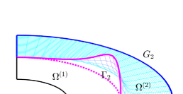
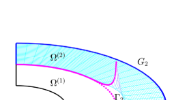
Figure 4: The lifting $\overline{\cal L}^{(2)}\mu_{j}^{(2)}$. At left, $\mu_{j}^{(2)}$ (the purple function defined on $\Gamma_{2}$) is identically null on $\partial\Gamma_{2}$ and $\overline{\cal L}^{(2)}\mu_{j}^{(2)}$ is identically null on $G_{2}=\partial\Omega^{(2)}\setminus\Gamma_{2}$ ($G_{2}$ is drawn in blue); at right, $\mu_{j}^{(2)}$ is not identically null on $\partial\Gamma_{2}$ and $\overline{\cal L}^{(2)}\mu_{j}^{(2)}$ is not identically null on $G_{2}$.

For $k=1,2$ we denote by ${\bf r}_{\overline{\Gamma}_{k}}$ the array whose entries are the real values $r_{i}^{(k)}$, for $i=1,\ldots,n^{(k)}_{\Gamma}$ and, following the nomenclature used in linear algebra, ${\bf r}_{\overline{\Gamma}_{k}}$ is named residual vector.

The values $r^{(k)}_{i}$ are not the coefficients of the primal expansion of $\frac{\partial u_{h_{k}}^{(k)}}{\partial{\bf n}_{k}}$, so we cannot apply the interpolation matrix $P_{\ell k}$ to the array ${\bf r}_{\overline{\Gamma}_{k}}$. Rather they are the coefficients of $\frac{\partial u_{h_{k}}^{(k)}}{\partial{\bf n}_{k}}$ with respect to the basis $\{\Phi_{j}^{(k)}\}_{j=1}^{n^{(k)}_{\Gamma}}$ in $(Y_{h_{k}}^{(k)})^{\prime}$ that is dual to $\{\mu_{j}^{(k)}\}_{j=1}^{n^{(k)}_{\Gamma}}$ (see, e.g. [21, 4]), i.e. satisfying

$$\langle\Phi_{j}^{(k)},\mu_{i}^{(k)}\rangle=\int_{\Gamma_{k}}\Phi_{j}^{(k)}\,\mu_{i}^{(k)}d\Gamma=\delta_{ij},\qquad i,j=1,\ldots,n^{(k)}_{\Gamma}$$

(where $\delta_{ij}$ is the Kronecker delta), and it holds

$$\frac{\partial u_{h_{k}}^{(k)}}{\partial{\bf n}_{k}}=\sum_{j=1}^{n^{(k)}_{\Gamma}}r^{(k)}_{j}\Phi_{j}^{(k)}.$$ (66)

Nevertheless, $Y_{h_{k}}^{(k)}$ and $(Y_{h_{k}}^{(k)})^{\prime}$ are the same (finite dimensional) algebraic space ([4]) and we denote by ${\cal J}_{k}$ the canonical isomorphism between $Y_{h_{k}}^{(k)}$ and its dual $(Y_{h_{k}}^{(k)})^{\prime}$.

To transfer the normal derivative $\frac{\partial u^{(2)}_{h_{2}}}{\partial{\bf n}_{2}}$ from $\Gamma_{2}$ to $\Gamma_{1}$, we define the operator $\widetilde{\Pi}_{12}:(Y_{h_{2}}^{(2)})^{\prime}\to(Y_{h_{1}}^{(1)})^{\prime}$ such that $\widetilde{\Pi}_{12}={\cal J}_{1}\Pi_{12}{\cal J}_{2}^{-1},$ i.e.

The interface mass matrix $M_{\Gamma_{k}}$ on $\Gamma^{(k)}$, whose entries are

$$(M_{\Gamma_{k}})_{ij}=(\mu_{j}^{(k)},\mu_{i}^{(k)})_{L^{2}(\Gamma_{k})},\qquad i,j=1,\ldots,n^{(k)}_{\Gamma},$$ (67)

is the matrix corresponding to the isomorphism ${\cal J}_{k}$.

Assume that $u^{(2)}_{h_{2}}$ is known, the computation of $\widetilde{\Pi}_{12}\frac{\partial u_{h_{2}}^{(2)}}{\partial{\bf n}_{2}}$ is carried out as follows:

1. compute the entries of the array ${\bf r}_{\overline{\Gamma}_{2}}$ by (65);

2. compute the array ${\bf z}_{\overline{\Gamma}_{2}}=M_{\Gamma_{2}}^{-1}{\bf r}_{\overline{\Gamma}_{2}},$ the entries of ${\bf z}_{\overline{\Gamma}_{2}}$ are in fact the coefficients of the expansion (named $z_{h_{2}}^{(2)}$) of $\frac{\partial u_{h_{2}}^{(2)}}{\partial{\bf n}_{2}}$ with respect to the primal basis $\mu_{j}^{(2)}$ of $Y_{h_{2}}^{(2)}$ (see, e.g., [21, 4]);

3. compute the array ${\bf s}_{\overline{\Gamma}_{1}}=P_{12}{\bf z}_{\overline{\Gamma}_{2}},$ the entries of ${\bf s}_{\overline{\Gamma}_{1}}$ are the primal coefficients of the function $s=\Pi_{12}z_{h_{2}}^{(2)}\in Y_{h_{1}}^{(1)}$;

4. compute the array $\breve{\bf r}_{\overline{\Gamma}_{1}}=M_{\overline{\Gamma}_{1}}{\bf s}_{\overline{\Gamma}_{1}},$ i.e., come back to the dual expansion.

The entries of the array

$$\breve{\bf r}_{\overline{\Gamma}_{1}}=M_{\Gamma_{1}}P_{12}M_{\Gamma_{2}}^{-1}{\bf r}_{\overline{\Gamma}_{2}}$$ (68)

are the coefficients of the expansion of $\widetilde{\Pi}_{12}\frac{\partial u^{(2)}_{h_{2}}}{\partial{\bf n}_{2}}$ with respect to the dual basis $\{\Phi_{j}^{(1)}\}$, i.e.,

$$\widetilde{\Pi}_{12}\displaystyle\frac{\partial u^{(2)}_{h_{2}}}{\partial{\bf n}_{2}}=\sum_{j=1}^{n_{\Gamma}^{(1)}}\breve{r}_{j}\Phi_{j}^{(1)},\quad\mbox{ and }\quad\langle\widetilde{\Pi}_{12}\displaystyle\frac{\partial u^{(2)}_{h_{2}}}{\partial{\bf n}_{2}},\mu_{i}^{(1)}\rangle=\breve{r}_{i}.$$ (69)

In conclusion, in view of (66) and (69), the algebraic counterpart of the interface condition (21)₃ reads

$${\bf r}_{\overline{\Gamma}_{1}}+M_{\Gamma_{1}}P_{12}M_{\Gamma_{2}}^{-1}{\bf r}_{\overline{\Gamma}_{2}}={\bf 0}.$$ (70)

5 The algebraic form of INTERNODES

For $k=1,2$ we define the following sets of indices:

–

${\cal I}_{\overline{\Omega}^{(k)}}=\{1,\ldots,N^{(k)}\}$;

–

${\cal I}_{k}$ the subset of the indices of ${\cal I}_{\overline{\Omega}^{(k)}}$ associated with the basis functions of ${\cal N}^{(k)}_{h_{k}}$ that are identically null on $\partial\Omega^{(k)}$;

–

${\cal I}_{\overline{\Gamma}_{k}}$ the subset of the indices of ${\cal I}_{\overline{\Omega}^{(k)}}$ associated with the basis functions of ${\cal N}^{(k)}_{h_{k}}$ that are not identically null on $\Gamma_{k}$ (even if $\Gamma_{k}=\overline{\Gamma}_{k}$, the bar over $\Gamma_{k}$ stresses the fact that we are taking into account for all the basis functions that are not identically null on $\overline{\Gamma}_{k}$);

–

${\cal I}_{\Gamma_{k}}$ the subset of the indices of ${\cal I}_{\overline{\Omega}^{(k)}}$ associated with the basis functions of ${\cal N}^{(k)}_{h_{k}}$ that are not identically null on the interior of $\Gamma_{k}$ and are identically null on $\partial\Gamma_{k}$;

–

${\cal I}_{D_{k}}$ the subset of the indices of ${\cal I}_{\overline{\Omega}^{(k)}}$ associated with the Dirichlet degrees of freedom;

–

${\cal I}_{\partial\Gamma_{k}}={\cal I}_{\overline{\Gamma}_{k}}\setminus{\cal I}_{\Gamma_{k}}$.

We define the local stiffness matrices $A^{(k)}$ whose entries are

$$A^{(k)}_{ij}=a^{(k)}(\varphi_{j},\varphi_{i}),\qquad i,j\in{\cal I}_{\overline{\Omega}^{(k)}},$$ (71)

then let

$$A^{(k,k)}=A^{(k)}({\cal I}_{k},{\cal I}_{k})$$

be the submatrix of $A^{(k)}$ obtained by taking both rows and columns of $A^{(k)}$ whose indices belong to ${\cal I}_{k}$. Similarly, we define the submatrices $A^{(k,\Gamma_{k})}=A^{(k)}({\cal I}_{k},{\cal I}_{\Gamma_{k}})$, $A^{(\Gamma_{k},\Gamma_{k})}=A^{(k)}({\cal I}_{\Gamma_{k}},{\cal I}_{\Gamma_{k}}),$ $A^{(\overline{\Gamma}_{k},k)}=A^{(k)}({\cal I}_{\overline{\Gamma}_{k}},{\cal I}_{k})$, $A^{(\overline{\Gamma}_{k},D_{k})}=A^{(k)}({\cal I}_{\overline{\Gamma}_{k}},{\cal I}_{D_{k}})$, $A^{(\overline{\Gamma}_{k},\overline{\Omega}^{(k)})}=A^{(k)}({\cal I}_{\overline{\Gamma}_{k}},{\cal I}_{\overline{\Omega}^{(k)}})$, and so on.

Moreover, we define the array ${\bf f}^{(k)}$ whose entries are

$$f^{(k)}_{i}={\cal F}_{k}(\varphi_{i}^{(k)}),\qquad i\in{\cal I}_{\overline{\Omega}^{(k)}},$$

the array ${\bf u}^{(k)}$ of the degrees of freedom in $\overline{\Omega}^{(k)}$, and using the same notation as above, the subarrays

$$\begin{array}[]{lll}{\bf f}^{(k)}_{0}={\bf f}^{(k)}({\cal I}_{k}),&{\bf f}_{\overline{\Gamma}_{k}}={\bf f}^{(k)}({\cal I}_{\overline{\Gamma}_{k}}),&{\bf f}_{\Gamma_{k}}={\bf f}^{(k)}({\cal I}_{\Gamma_{k}}),\\[2.84526pt] {\bf u}^{(k)}_{0}={\bf u}^{(k)}({\cal I}_{k}),&{\bf u}_{\overline{\Gamma}_{k}}={\bf u}^{(k)}({\cal I}_{\overline{\Gamma}_{k}}),&{\bf u}_{\Gamma_{k}}={\bf u}^{(k)}({\cal I}_{\Gamma_{k}}).\end{array}$$

Finally, we denote by ${\bf g}_{k}$ and ${\bf g}_{\partial\Gamma_{k}}$ the arrays of all the Dirichlet degrees of freedom associated with $\partial\Omega^{(k)}_{D}$ and $\partial\Gamma_{k}$, respectively.

To evaluate the last integral of (65) we define the matrix $C^{(k)}$ whose non-null entries are

$$\begin{array}[]{lll}C^{(k)}_{ij}&\displaystyle=-\int_{G_{k}}\frac{\partial\varphi_{j}^{(k)}}{\partial{\bf n}_{k}}\varphi_{i}^{(k)},&\mbox{ for }i\in{\cal I}_{\partial\Gamma_{k}},\ j\in{\cal I}_{\overline{\Omega}^{(k)}}\end{array}$$ (74)

and, as done for the stiffness matrix $A^{(k)}$, we set $C^{(\Gamma_{k},k)}=C^{(k)}({\cal I}_{\Gamma_{k}},{\cal I}_{k}),$ $C^{(\Gamma_{k},\Gamma_{k})}=C^{(k)}({\cal I}_{\Gamma_{k}},{\cal I}_{\Gamma_{k}}),$ $C^{(\Gamma_{k},D_{k})}=C^{(k)}({\cal I}_{\Gamma_{k}},{\cal I}_{D_{k}})$, and so on.

The integrals in (74) can be easily computed by exploiting the definition of the NURBS basis functions, moreover the rows of $C^{(k)}$ associated with all the degrees of freedom not belonging to ${\cal I}_{\partial\Gamma_{k}}$ are null. Thus the computation of $C^{(k)}$ is very cheap.

Then we define

$$\widehat{A}^{(\Gamma_{k},X)}=A^{(\Gamma_{k},X)}+C^{(\Gamma_{k},X)}\quad\mbox{and}\quad\widehat{A}^{(\overline{\Gamma}_{k},X)}=A^{(\overline{\Gamma}_{k},X)}+C^{(\overline{\Gamma}_{k},X)},$$ (75)

where $X\in\{\overline{\Omega}^{(k)},\ k,\ \Gamma_{k},\ \overline{\Gamma}_{k},\ D_{k}\}$, so that the algebraic implementation of (65) reads, for $k=1,2$,

$${\bf r}_{\overline{\Gamma}_{k}}=\widehat{A}^{(\overline{\Gamma}_{k},\overline{\Omega}^{(k)})}{\bf u}^{(k)}-{\bf f}_{\overline{\Gamma}_{k}}.$$ (76)

By defining the two intergrid matrices

$$Q_{21}=P_{21},\qquad Q_{12}=M_{\Gamma_{1}}P_{12}M_{\Gamma_{2}}^{-1},$$ (77)

the algebraic counterpart of (21)_2,3 read (see (51) and (70))

$$\begin{array}[]{l}{\bf u}_{\overline{\Gamma}_{2}}=Q_{21}{\bf u}_{\overline{\Gamma}_{1}},\qquad\qquad{\bf r}_{\overline{\Gamma}_{1}}+Q_{12}{\bf r}_{\overline{\Gamma}_{2}}={\bf 0}.\end{array}$$ (79)

By introducing the following submatrices:

$$Q_{21}^{(\overline{\Gamma}_{2},\Gamma_{1})}=Q_{21}({\cal I}_{\overline{\Gamma}_{2}},{\cal I}_{\Gamma_{1}}),\quad Q_{21}^{(\Gamma_{2},\partial\Gamma_{1})}=Q_{21}({\cal I}_{\Gamma_{2}},{\cal I}_{\partial\Gamma_{1}}),\quad Q_{12}^{(\Gamma_{1},\overline{\Gamma}_{2})}=Q_{12}({\cal I}_{\Gamma_{1}},{\cal I}_{\overline{\Gamma}_{2}}),$$

and by using (79), the algebraic form of (21) reads

$$\underbrace{\left[\begin{array}[]{ccc}A^{(1,1)}&0&A^{(1,\Gamma_{1})}\\[2.84526pt] 0&A^{(2,2)}&A^{(2,\overline{\Gamma}_{2})}Q_{21}^{(\overline{\Gamma}_{2},\Gamma_{1})}\\[2.84526pt] \widehat{A}^{(\Gamma_{1},1)}&Q_{12}^{(\Gamma_{1},\overline{\Gamma}_{2})}\widehat{A}^{(\overline{\Gamma}_{2},2)}&\widehat{A}^{(\Gamma_{1},\Gamma_{1})}+Q_{12}^{(\Gamma_{1},\overline{\Gamma}_{2})}\widehat{A}^{(\overline{\Gamma}_{2},\overline{\Gamma}_{2})}Q_{21}^{(\overline{\Gamma}_{2},\Gamma_{1})}\end{array}\right]}_{\displaystyle\mathbb{A}}\left[\!\!\begin{array}[]{l}{\bf u}^{(1)}_{0}\\[2.84526pt] {\bf u}^{(2)}_{0}\\[2.84526pt] {\bf u}_{\Gamma_{1}}\end{array}\!\!\right]=\left[\!\!\begin{array}[]{c}{\bf f}^{(1)}_{0}\\[2.84526pt] {\bf f}^{(2)}_{0}\\[2.84526pt] {\bf f}_{\Gamma_{1}}+Q_{12}^{(\Gamma_{1},\overline{\Gamma}_{2})}{\bf f}_{\overline{\Gamma}_{2}}\end{array}\!\!\right]-{\bf G},$$ (89)

where the array

$${\bf G}=\left[\begin{array}[]{c}{\bf G}_{1}\\ {\bf G}_{2}\\ {\bf G}_{\Gamma_{1}}\end{array}\right]=\left[\begin{array}[]{c}A^{(1,D_{1})}{\bf g}_{1}\\[2.84526pt] A^{(2,D_{2})}{\bf g}_{2}+A^{(2,\Gamma_{2})}Q_{21}^{(\Gamma_{2},\partial\Gamma_{1})}{\bf g}_{\partial\Gamma_{1}}\\[2.84526pt] \widehat{A}^{(\Gamma_{1},D_{1})}{\bf g}_{1}+Q_{12}^{(\Gamma_{1},\overline{\Gamma}_{2})}(\widehat{A}^{(\overline{\Gamma}_{2},D_{2})}{\bf g}_{2}+\widehat{A}^{(\overline{\Gamma}_{2},\Gamma_{2})}Q_{21}^{(\Gamma_{2},\partial\Gamma_{1})}{\bf g}_{\partial\Gamma_{1}})\end{array}\right]$$ (96)

is non null only when non-homogeneous Dirichlet conditions are given on $\partial\Omega_{D}$ and implements the lifting of the Dirichlet datum.

Finally the degrees of freedom in $\Omega^{(1)}$ are given by ${\bf u}^{(1)}=[{\bf u}^{(1)}_{0},\ {\bf u}_{\Gamma_{1}},\ {\bf g}_{1}]$ while the one in $\Omega^{(2)}$ are given by ${\bf u}^{(2)}=[{\bf u}^{(2)}_{0},\ Q_{21}^{(\Gamma_{2},\overline{\Gamma}_{1})}{\bf u}_{\overline{\Gamma}_{1}},{\bf g}_{2}]$.

The presence of the terms $\widehat{A}^{(\overline{\Gamma}_{2},\Gamma_{2})}Q_{21}^{(\Gamma_{2},\partial\Gamma_{1})}{\bf g}_{\partial\Gamma_{1}}$ and $A^{(2,\Gamma_{2})}Q_{21}^{(\Gamma_{2},\partial\Gamma_{1})}{\bf g}_{\partial\Gamma_{1}}$ in the last two rows of (96) is motivated by the fact that the trace of $u^{(2)}_{h_{2}}$ on the interface $\Gamma_{2}$ is the interpolation through $\Pi_{21}$ of the trace of $u^{(1)}_{h_{1}}$ on $\Gamma_{1}$.

System (89) represents the algebraic form of INTERNODES implemented in practice. By taking $Q_{12}=Q_{21}=I$ we recover the algebraic system associated with classical conforming domain decomposition (see, e.g., [40, 44]).

Notice that, even though the residuals are defined up to the boundary of $\Gamma_{k}$, the algebraic counterpart of condition (21)₃ is imposed only on the degrees of freedom internal to $\Gamma_{1}$. In this way the number of equations and the number of unknowns in (89) do coincide.

5.1 An iterative method to solve (89)

An alternative way to solve system (89) consists in eliminating the variables ${\bf u}^{(1)}_{0}$ and ${\bf u}^{(2)}_{0}$ and in solving the Schur complement system ([44, 40])

$$S{\bf u}_{\Gamma_{1}}={\bf b},$$ (97)

where

$$S=S_{\Gamma_{1}}+Q_{12}^{(\Gamma_{1},\overline{\Gamma}_{2})}S_{\overline{\Gamma}_{2}}Q_{21}^{(\overline{\Gamma}_{2},\Gamma_{1})}, {\bf b}={\bf b}_{\Gamma_{1}}+Q_{12}^{(\Gamma_{1},\overline{\Gamma}_{2})}{\bf b}_{\overline{\Gamma}_{2}}-{\bf G}_{\Gamma_{1}},$$ (98)

$$S_{\Gamma_{1}}=\widehat{A}^{(\Gamma_{1},\Gamma_{1})}-\widehat{A}^{(\Gamma_{1},1)}(A^{(1,1)})^{-1}A^{(1,\Gamma_{1})}, S_{\overline{\Gamma}_{2}}=\widehat{A}^{(\overline{\Gamma}_{2},\overline{\Gamma}_{2})}-\widehat{A}^{(\overline{\Gamma}_{2},2)}(A^{(2,2)})^{-1}A^{(2,\overline{\Gamma}_{2})}$$ (99)

$${\bf b}_{\Gamma_{1}}={\bf f}_{\Gamma_{1}}-\widehat{A}^{(\Gamma_{1},1)}(A^{(1,1)})^{-1}({\bf f}^{(1)}_{0}-{\bf G}_{1}), {\bf b}_{\overline{\Gamma}_{2}}={\bf f}_{\overline{\Gamma}_{2}}-\widehat{A}^{(\overline{\Gamma}_{2},2)}(A^{(2,2)})^{-1}({\bf f}^{(2)}_{0}-{\bf G}_{2}).$$ (100)

$S_{\Gamma_{1}}$ and $S_{\overline{\Gamma}_{2}}$ are the local Schur complement matrices, while ${\bf b}_{\Gamma_{1}}$ and ${\bf b}_{\overline{\Gamma}_{2}}$ are the local right hand sides.

System (97) can be solved, e.g., by a preconditioned Krylov method (Bi-CGStab or GMRES) with $S_{1}$ as preconditioner. Notice that the matrix $Q_{12}^{(\Gamma_{1},\overline{\Gamma}_{2})}S_{\overline{\Gamma}_{2}}Q_{21}^{(\overline{\Gamma}_{2},\Gamma_{1})}$ is not a good candidate to play the role of preconditioner since it may be singular.

Since $Q_{12}$ is not the transpose of $Q_{21}$, even if the differential operator is symmetric, the Schur complement system $S$ is not. Nevertheless the local systems continue to be symmetric and can be solved either by standard Cholesky factorization or the PCG method. For example, we can compute and store the Cholesky factorization of the matrices $A^{(k,k)}$ and dispose of a function that implements the action of $S$ on a given array ${\boldsymbol{\lambda}}$ whose entries are the degrees of freedom associated with $\Gamma_{1}$.

We will describe the iterative approach in Sect. 9 for general multipatch configurations.

Once ${\bf u}_{\Gamma_{1}}$ is known, the variables ${\bf u}^{(1)}_{0}$ and ${\bf u}^{(2)}_{0}$ are recovered by solving the local subsystems

$$A^{(1,1)}{\bf u}^{(1)}_{0} = {\bf f}^{(1)}_{0}-{\bf G}_{1}-A^{(1,\Gamma_{1})}{\bf u}_{\Gamma_{1}},$$

$$A^{(2,2)}{\bf u}^{(2)}_{0} = {\bf f}^{(2)}_{0}-{\bf G}_{2}-A^{(2,\overline{\Gamma}_{2})}Q_{21}^{(\overline{\Gamma}_{2},\Gamma_{1})}{\bf u}_{\Gamma_{1}}.$$

Finally, ${\bf u}_{\overline{\Gamma}_{1}}$ is recovered by assembling ${\bf u}_{\Gamma_{1}}$ and ${\bf g}_{\partial\Gamma_{1}}$ and the numerical solution on $\overline{\Gamma}_{2}$ is reconstructed by the interpolation formula ${\bf u}_{\overline{\Gamma}_{2}}=Q_{21}{\bf u}_{\overline{\Gamma}_{1}}$.

6 Numerical results for 2 patches

The aim of this section is twofold. From one hand we show that INTERNODES does not deteriorate the accuracy of IGA discretization (we say that the method exhibits optimal accuracy). Then we show that, if the interfaces are non-watertight, the accuracy of the INTERNODES solution depends on the maximum size $d_{\Gamma}$ of gaps and overlaps between $\Gamma_{1}$ and $\Gamma_{2}$, and smaller $d_{\Gamma}$, smaller the error.

To highlight these features of INTERNODES we consider here very regular solutions. Other test case with less regular solutions will be taken into account in Sect. 10 in the case of $M>2$ patches.

6.1 Test case #1.

Let us consider the differential problem (3) in $\Omega=\{(x,y)\in{\mathbb{R}}^{2}:\ x\geq 0,\ y\geq 0,\ 1\leq x^{2}+y^{2}\leq 4\}$ with $\alpha=0$, and $f$ and $g$ such that the exact solution is $u(x,y)=\sin(1.5\pi x)\sin(3\pi y)$.

The computational domain $\Omega$ is split into the patches $\Omega^{(1)}=\{(x,y)\in\Omega:\ x^{2}+y^{2}\leq(1.5)^{2}\}$ and $\Omega^{(2)}=\{(x,y)\in\Omega:\ (1.5)^{2}\leq x^{2}+y^{2}\leq 4\}$ (see Fig. 5). Each patch is parameterized by NURBS as described in Sect. 4. The weights and the control points of the circular arcs are chosen as described in [9, Sect. 2.4.1.1]; each patch is built first as a single element with 6 control points, more precisely:

${\bf P}_{i}^{(1)}$	(1,0)	(1.5,0)	(0,1)	(1,1)	(0,1.5)	(1.5,1.5)
${\bf P}_{i}^{(2)}$	(1.5,0)	(2,0)	(0,1.5)	(1.5,1.5)	(0,2)	(2,2)
$w_{i}^{(1)}=w_{i}^{(2)}$	1	1	1	$\sqrt{2}/2$	1	$\sqrt{2}/2$,

then it is ${\sf k}-$refined (see [9, Sect. 2.1.4.3]) up to polynomial degree $p^{(k)}$ and continuity order $p^{(k)}-1$ along both the coordinates, and finally it is uniformly $h-$refined leaving the underlying geometry and its parametrization intact (see [9, Sect. 2.1.4.1]).

Then, let

$$u_{h}=\left\{\begin{array}[]{ll}u_{h_{1}}^{(1)}&\mbox{ in }\Omega^{(1)}\\ u_{h_{2}}^{(2)}&\mbox{ in }\Omega^{(2)}\end{array}\right.$$ (103)

denote the numerical solution computed with INTERNODES.

We consider three non-matching parametrizations named: balanced, master-refined and slave-refined (in fact these are $h-$refinements). We take equal polynomial degrees $p^{(1)}=p^{(2)}=p\in\{2,\ldots,5\}$ and, for $\overline{n}\in\{8,16,24,32\}$, we define the number of elements inside the patches as follows:

patch	balanced	master-refined	slave-refined
$\Omega^{(1)}$	$(\overline{n}/2)\times\overline{n}$	$(\overline{n}-1)\times 2(\overline{n}-1)$	$(\overline{n}/2)\times\overline{n}$
$\Omega^{(2)}$	$\overline{n}/2\times(\overline{n}+1)$	$(\overline{n}/2)\times\overline{n}$	$\overline{n}\times(2\overline{n}+1)$.

The first (second, resp.) parameter coordinate is mapped onto the physical radial (angular, resp.) coordinate, and the non-conformity is a consequence of the different number of elements along the second coordinate.

In Fig. 5, we show the the three discretization sets when $\overline{n}=8$, while in Fig. 6 we show the broken-norm errors

$$\|u_{h}-u\|_{*}=\left(\sum_{k}\frac{\|u_{h}-u\|^{2}_{H^{1}(\Omega^{(k)})}}{\|u\|^{2}_{H^{1}(\Omega^{(k)})}}\right)^{1/2}$$ (104)

with respect to the maximum mesh size $h=\max_{k}h_{k}$ ($h_{k}$ is the mesh-size in $\Omega^{(k)}$), for the three discretization sets.

The convergence of INTERNODES is optimal versus the mesh-size $h$, in the sense that the broken-norm errors behave like $h^{p}$ when $h\to 0$, exactly as the error in $H^{1}-$norm of the Galerkin Isogeometric methods (see, e.g., [13, Thm. 3.4 and Cor. 4.16]).

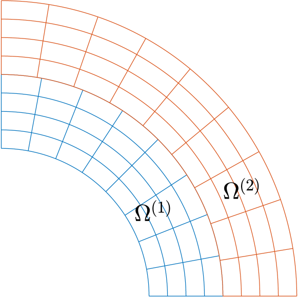
(a)

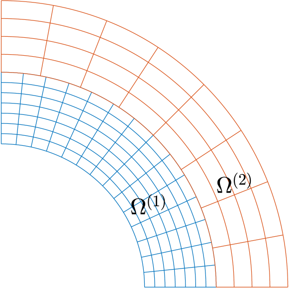
(b)

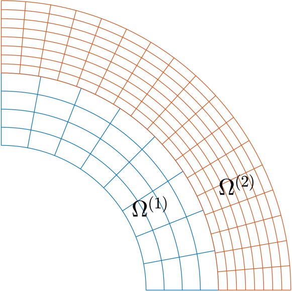
(c)

Figure 5: Test case #1. Balanced (a), master-refined (b), slave-refined (c) discretization sets with $\overline{n}=8$

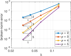
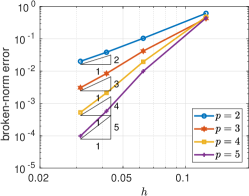
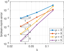
Figure 6: Test case #1. The broken-norm error (104) versus the mesh size. At left the error for the balanced configuration, in the middle the error for the master-refined configuration, at right the error for the slave-refined configuration

In Fig. 7 we show the broken-norm errors versus the polynomial degree $p^{(1)}$, with three different choices for $p^{(2)}$: $p^{(2)}=p^{(1)}$, $p^{(2)}=p^{(1)}+1$ and $p^{(2)}=p^{(1)}+2$ and the discretization sets: balanced and slave refined. In all the cases $\overline{n}=20$. Finally, in Fig. 8, we present two qualitative pictures of the INTERNODES solution.

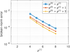
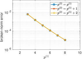
Figure 7: Test case #1. The broken-norm error versus the polynomial degree $p^{(1)}$ in the patch $\Omega^{(1)}$. At left the error for the balanced configuration at right the error for the slave refined configuration, $\overline{n}=20$ for both cases

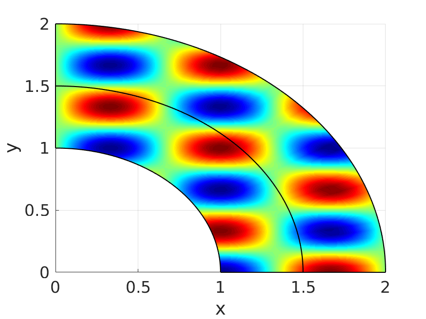
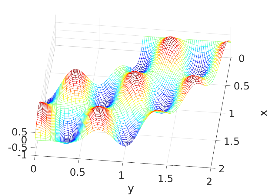
Figure 8: Test case #1. The numerical solution obtained with $p^{(1)}=p^{(2)}=3$, $(8\times 16)$ elements in $\Omega^{(1)}$, and $(8\times 17)$ elements in $\Omega^{(2)}$. The first (second, resp.) parameter coordinate is mapped on the physical radial (angular, resp.) coordinate. The number of grid points used in the right plot is about twice the number of degrees of freedom

6.2 Test case #2. Non-watertight patches

Let us consider the differential problem (3) in $\Omega=(0,2)\times(0,1)$ with $\alpha=0$, and $f$ and $g$ such that the exact solution is $u(x,y)=e^{-3(x-1)^{2}-4(y-0.6)^{2}}(1+\sin(3\pi x)\cos(3\pi y)).$

The computational domain $\Omega$ is split into two patches as shown in Fig. 9, left, where we have considered a sinusoidal physical interface $\Gamma_{12}=\{(x,y)\in{\mathbb{R}}^{2}:\ x=g(y)=1+0.2\sin(2\pi y),\ 0\leq y\leq 1\}$. The interfaces $\Gamma_{1}$ and $\Gamma_{2}$ are built as B-spline interpolation of $\Gamma_{12}$ and they are non-watertight. The size of gaps and overlaps that are generated by the approximation (we denote by $d_{\Gamma}$ the maximum distance between the two interfaces) depends on the parameterization of the patches. To face the non-watertight interfaces we implement INTERNODES with the RL-RBF interpolation operators defined in Sect. 4.3.

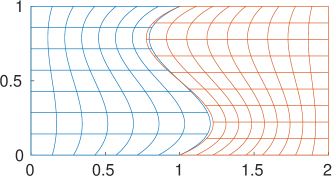
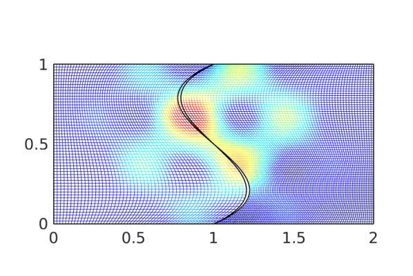
Figure 9: Test case #2. At left, the parameterization of the two patches with $7\times 7$ elements in $\Omega^{(1)}$ and $9\times 9$ elements in $\Omega^{(2)}$. The maximum distance between $\Gamma_{1}$ and $\Gamma_{2}$ is $d_{\Gamma}=0.0197$. At right the numerical solution computed by INTERNODES (with RL-RBF interpolation) with $p^{(1)}=4$ and $p^{(2)}=3$. The number of grid points used in the plot is about four times the number of degrees of freedom

We analyze the accuracy of INTERNODES by measuring the broken-norm error (104) versus the mesh size $h=\max_{k}h_{k}$ in two situations: i) with fixed $d_{\Gamma}$, ii) with variable $d_{\Gamma}$.

i) Fixed $d_{\Gamma}$. We fix two different polynomial degrees $p^{(1)}$ and $p^{(2)}$, thus for $k=1,2$ we determine the interfaces $\Gamma_{k}$ as follows:

1. let $\Xi^{(k)}=\{\underbrace{0\ldots 0}_{p^{(k)}},\underbrace{1\ldots 1}_{p^{(k)}}\}$ be the knots set on a single element,

2. let $\widehat{\varphi}_{i,p^{(k)}}^{(k)}$ denote the univariate B-spline basis functions of degree $p^{(k)}$ associated with $\Xi^{(k)}$,

3. let $\widehat{t}_{j,G}^{(k)}$, for $j=1,\ldots,p^{(k)}+1$ the Greville abscissae associated with $\Xi^{(k)}$,

4. let ${\bf Q}_{j}^{(k)}=(g(\widehat{t}_{j,G}^{(k)}),\widehat{t}_{j,G}^{(k)})$, for $j=1,\ldots,p^{(k)}+1$,

5. compute the points ${\bf P}_{i}^{(k)}$, for $i=1,\ldots p^{(k)}+1$, by solving the linear system (see, e.g. [38, Sect. 9.2.1])

   $$\sum_{i=1}^{p^{(k)}+1}\widehat{\varphi}_{i,p^{(k)}}^{(k)}(\widehat{t}_{j,G}^{(k)}){\bf P}_{i}^{(k)}={\bf Q}_{j}^{(k)},\qquad j=1,\ldots,p^{(k)}+1.$$ (105)

The points ${\bf P}_{i}^{(k)}$ are in fact the control points of the curve that defines $\Gamma_{k}$. We have chosen the associated weights equal to 1 (but different weights can be chosen as well providing NURBS instead of B-spline parametrization), the parameterization of the patch $\Omega^{(k)}$ can be defined as ruled surface between $\Gamma_{k}$ and the opposite straight side. Finally, uniform $h-$refinement is adopted to reach the desired final discretization, while the polynomial degrees remain fixed.

ii) Variable $d_{\Gamma}$. In this case we choose equal polynomial degrees $p^{(1)}=p^{(2)}$. Moreover, the initial set $\Xi^{(k)}$ includes all the knots corresponding to the desired uniform $h-$refinement. Then we proceed as in case i), by omitting the final $h-$refinement.

For the case i) we have chosen three couples of polynomial degrees: the first one with $p^{(1)}=5$ and $p^{(2)}=3$ that provides $d_{\Gamma}=0.055$; the second one with $p^{(1)}=4$ and $p^{(2)}=3$ that provides $d_{\Gamma}=0.0197$; the third one with $p^{(1)}=6$ and $p^{(2)}=5$ that provides $d_{\Gamma}=0.0018$. In the left picture of Fig. 10 we plot the broken-norm errors versus the mesh size $h=\max_{k}h_{k}$; we have taken $(\overline{n}-1)\times(\overline{n}-1)$ elements in $\Omega^{(1)}$ and $(\overline{n}+1)\times(\overline{n}+1)$ elements in $\Omega^{(1)}$. The plateaux in the error curves are clearly due to the presence of non-watertight interfaces and, smaller $d_{\Gamma}$, lower the plateau.

For the case ii) we have chosen $p=p^{(1)}=p^{(2)}\in\{2,\ldots,5\}$ and different values of $h=\max_{k}h_{k}$. In this case the maximum size $d_{\Gamma}$ of gaps and overlaps decreases as $h^{p}$ (in fact it corresponds to the B-spline interpolation error of the curve $g(y)$). In the right picture of Fig. 10 the corresponding broken-norm errors are shown, they decrease like $h^{p}$ when $h\to 0$, as in the case of watertight interfaces.

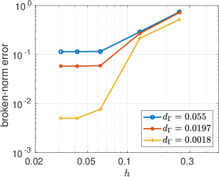
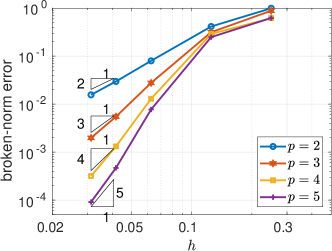
Figure 10: Test case #2. At left, the errors for the case i): $p^{(1)}=5$ and $p^{(2)}=3$ when $d_{\Gamma}=0.055$; $p^{(1)}=4$ and $p^{(2)}=3$ when $d_{\Gamma}=0.0197$; $p^{(1)}=6$ and $p^{(2)}=5$ when $d_{\Gamma}=0.0018$. At right, the errors for the case ii) with $p=p^{(1)}=p^{(2)}$ and $d_{\Gamma}={\cal O}(h^{p})$

We have solved the Schur complement system (97) by the preconditioned Bi-CGStab (PBi-CGStab) method as mentioned in Sect. 5.1, with preconditioner $P$ given by the local Schur complement matrix $S_{\Gamma_{1}}$. It is well known (see, e.g., [40]) that, in the framework of conforming Finite Element/Spectral Element discretizations, such a preconditioner is optimal, that is the condition number of $(S_{\Gamma_{1}})^{-1}S$ is bounded independently of the mesh size and the polynomial degree. Our numerical results show that this preconditioner looks optimal also for non-matching NURBS parametrizations.

In Table 1 we report the number of iterations required by the PBi-CGStab to solve the Schur complement system (97) up to a tolerance $\epsilon=10^{-10}$. In the right picture of Fig. 9 the INTERNODES solution obtained with RL-RBF interpolation is shown. We have set $p^{(1)}=5$, $p^{(2)}=3$, $7\times 7$ elements in $\Omega^{(1)}$ and $9\times 9$ elements in $\Omega^{(2)}$.

$\overline{n}$	$d_{\Gamma}=0.055$	$d_{\Gamma}=0.0197$	$d_{\Gamma}=0.0018$
$4$	6	5	7
$8$	7	6	7
$16$	8	8	7
$24$	9	8	7
$32$	9	9	7

$\overline{n}$	$p=2$	$p=3$	$p=4$	$p=5$
$4$	3	4	5	6
$8$	6	6	7	7
$16$	6	7	6	7
$24$	7	7	7	7
$32$	7	7	7	7

Table 1: Test case #2. The number of Bi-CGStab iterations required to solve the Schur complement system (97). The stop tolerance is $\epsilon=10^{-10}$. We have set $(\overline{n}-1)\times(\overline{n}-1)$ elements in $\Omega^{(1)}$ and $(\overline{n}+1)\times(\overline{n}+1)$ elements in $\Omega^{(2)}$. The left table refers to case i), while the right one to the case ii)

7 More general second order elliptic PDEs

INTERNODES methods can be applied to solve general elliptic second order PDEs, where the differential operator is

$$Lu=-\nabla\cdot(\nu\nabla u)+{\bf b}\cdot\nabla u+\alpha u,$$ (106)

with $\nu\in L^{\infty}(\Omega)$ such that there exists $\nu_{0}>0$ and $\nu\geq\nu_{0}$ a.e. in $\Omega$; ${\bf b}=(b_{1},\ldots,b_{d})$, with $b_{i}\in L^{\infty}(\Omega)$; $\alpha\in L^{\infty}(\Omega)$ with $\alpha\geq 0$ a.e. in $\Omega$.

Given $f\in L^{2}(\Omega)$ and $g\in H^{1/2}(\partial\Omega)$, and under the assumption that $\alpha-\frac{1}{2}\nabla\cdot{\bf b}\geq 0$ a.e. in $\Omega$, the problem to find $u\in H^{1}(\Omega)$ such that

$$\left\{\begin{array}[]{ll}Lu=f&\mbox{ in }\Omega\\ u=g&\mbox{ on }\partial\Omega\end{array}\right.$$ (109)

admits a unique solution that is stable w.r.t. the data $f$ and $g$.

In such a case, while the interface condition (9)₃ enforcing the continuity of the traces across $\Gamma_{12}$ does not change, the interface conditions (9)₄ involving the normal derivatives must be replaced by

$$\nu_{1}\frac{\partial u^{(1)}}{\partial{\bf n}_{1}}+\nu_{2}\frac{\partial u^{(2)}}{\partial{\bf n}_{2}}=0\qquad\mbox{ on }\Gamma_{12},$$ (110)

where $\nu_{k}=\nu_{|\Omega^{(k)}}$.

When Neumann boundary conditions are assigned on a subset $\partial\Omega_{N}$ of the boundary $\partial\Omega$, the definition of the set $G_{k}$ (that is used to define the real values $r_{i}^{(k)}$, see (65)) becomes $G_{k}=\partial\Omega^{(k)}\setminus(\Gamma_{k}\cup\partial\Omega_{N}),$ (see [24, formula (44)]).

8 INTERNODES for decompositions with $M\geq 2$ patches

Let now $\Omega^{(k)}$, with $k=1,\ldots,M$, denote a family of disjoint patches of $\Omega\subset{\mathbb{R}}^{d}$, with $d=2,3$, s.t. $\cup_{k}\overline{\Omega}^{(k)}=\overline{\Omega}$. Let us suppose that each $\Omega^{(k)}$ has Lipschitz boundary $\partial\Omega^{(k)}$ (for $k=1,\ldots,M$).

Let $\Gamma_{k}=\partial\Omega^{(k)}\setminus\partial\Omega$ be the part of the boundary of $\Omega^{(k)}$ internal to $\Omega$, and

$$\Gamma_{k\ell}=\Gamma_{\ell k}=\partial\Omega^{(k)}\cap\partial\Omega^{(\ell)}$$

be the interface between the two subdomains $\Omega^{(k)}$ and $\Omega^{(\ell)}$. Intersections having null measure in the topology of ${\mathbb{R}}^{d-1}$ are considered empty. Finally, let $L$ be the differential operator introduced in (106).

The multidomain formulation of problem (3) reads: look for $u^{(k)}$ for $k=1,\ldots,M$ such that:

$$\left\{\begin{array}[]{ll}Lu^{(k)}=f&\mbox{ in }\Omega^{(k)},\quad k=1,\ldots,M\\ u^{(k)}=g&\mbox{ on }\partial\Omega_{D}^{(k)},\\ u^{(k)}=u^{(\ell)},&\mbox{ on }\Gamma_{k\ell}\neq\emptyset,\ \ell=1,\ldots,M,\ \ell\neq k\\ \displaystyle\nu_{k}\frac{\partial u^{(k)}}{\partial{\bf n}_{k}}+\nu_{\ell}\frac{\partial u^{(\ell)}}{\partial{\bf n}_{\ell}}=0&\mbox{ on }\Gamma_{k\ell}\neq\emptyset,\ \ell=1,\ldots,M,\ \ell\neq k.\end{array}\right.$$ (115)

We split the internal boundary $\Gamma_{k}$ of $\partial\Omega^{(k)}$ in faces and we denote by $\gamma_{k,\alpha}$ the $\alpha$th face of $\Gamma_{k}$ (see Fig. 11 and Fig. 12), the first sub-index $k$ identifies the domain, while the second one $\alpha$ is the index of the face of $\Gamma_{k}$. As for the case of two subdomains, we assume that each interface $\gamma_{k,\ell}$ is sufficiently regular (i.e. of class $C^{1,1}$) to allow the conormal derivative of $u_{k}$ on $\gamma_{k,\ell}$ to be well defined.

Remark 8.1

We assume that $\gamma_{k,\alpha}$ includes its boundary.

For example, in the multipatch configuration of Fig. 11, we have $\Gamma_{1}=\gamma_{1,1}$, $\Gamma_{2}=\gamma_{2,1}\cup\gamma_{2,2}$ and $\Gamma_{3}=\gamma_{3,1}\cup\gamma_{3,2}$.

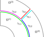
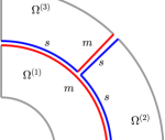
Figure 11: The physical domain $\Omega\subset{\mathbb{R}}^{2}$ split in 3 patches and the faces $\gamma_{k,\alpha}$. The interfaces $\Gamma_{k\ell}$ are: $\Gamma_{12}=\gamma_{1,1}\cap\gamma_{2,2}$, $\Gamma_{13}=\gamma_{1,1}\cap\gamma_{3,2}$, $\Gamma_{23}=\gamma_{2,1}\cap\gamma_{3,1}$. At right, a possible choice of the master/slave faces is shown

Moreover, for any face $\gamma_{k,\alpha}$ we define the set

$${\cal A}_{k,\alpha}=\{(\ell,\beta):\ \gamma_{\ell,\beta}\cap\gamma_{k,\alpha}\neq\emptyset\}$$ (116)

of the faces (of the other patches) that are adjacent to $\gamma_{k,\alpha}$. In the multipatch configuration of Fig. 11, we have ${\cal A}_{1,1}=\{(2,2),(3,2)\}$, ${\cal A}_{2,2}=\{(1,1)\}$, ${\cal A}_{2,1}=\{(3,1)\}$ and so on.

Between $\gamma_{k,\alpha}$ and $\gamma_{\ell,\beta}$, one is tagged as master and the other as slave and we define the master skeleton

$$\Gamma=\bigcup_{(k,\alpha)}\gamma_{k,\alpha}\quad\mbox{ with }\gamma_{k,\alpha}\mbox{ master.}$$ (117)

In the mortar community $\Gamma$ is named mortar interface.

A-priori there is no constraint in tagging a face as either master or slave. In the example of Fig. 11 right, we could tag as master the face $\gamma_{1,1}$ (in which case $\gamma_{2,2}$ and $\gamma_{3,2}$ will be both slave), or other way around.

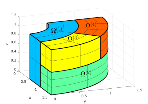
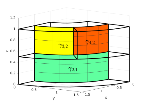
Figure 12: 3D-decompositions. $\gamma_{1,1}$ is the sole interface of $\Omega^{(1)}$ and it has non-null intersection with just one interface of each one of the other subdomains. $\Omega^{(2)}$ has two interfaces: $\gamma_{2,1}$ (that adjacent to $\Omega^{(1)}$) and $\gamma_{2,2}$ (the top one adjacent to both $\Omega^{(3)}$ and $\Omega^{(4)}$); $\Omega^{(3)}$ has three interfaces: $\gamma_{3,1}$ (that adjacent to $\Omega^{(4)}$), $\gamma_{3,2}$ (that adjacent to $\Omega^{(1)}$) and $\gamma_{3,3}$ (that adjacent to $\Omega^{(2)}$); $\Omega^{(4)}$ has three interfaces: $\gamma_{4,1}$ (that adjacent to $\Omega^{(3)}$), $\gamma_{4,2}$ (that adjacent to $\Omega^{(1)}$) and $\gamma_{4,3}$ (that adjacent to $\Omega^{(2)}$)

In the patch $\Omega^{(k)}$ we define a NURBS space ${\cal N}^{(k)}_{h_{k}}$ as defined in (34) and the corresponding finite dimensional spaces $V^{(k)}_{h_{k}}$ (see (17)) that are totally independent of the discretizations inside the adjacent patches. For each face $\gamma_{k,\alpha}\subset\Gamma_{k}$ we define the trace space

$$Y_{h_{k}}^{(k,\alpha)}=\{\lambda=v|_{\gamma_{k,\alpha}},\ v\in{\cal N}^{(k)}_{h_{k}}\}$$

whose dimension is denoted by $n^{(k,\alpha)}$.

The INTERNODES method for $M>2$ patches reads as follows. For $k=1,\ldots,M$, let $\widetilde{g}_{h_{k}}^{(k)}\in{\cal N}^{(k)}_{h_{k}}$ be a suitable approximation of $\widetilde{g}^{(k)}$, we look for $u^{(k)}_{h_{k}}\in{\cal N}^{(k)}_{h_{k}}$ such that $(u_{h_{k}}^{(k)}-\widetilde{g}_{h_{k}}^{(k)})\in V^{(k)}_{h_{k}}$ and

$$\left\{\begin{array}[]{ll}a^{(k)}(u_{h_{k}}^{(k)},v_{h_{k}}^{(k)})={\cal F}^{(k)}(v_{h_{k}}^{(k)})&\ \forall v_{h_{k}}^{(k)}\in V^{(k)}_{0,h_{k}},\\[8.53581pt] \mbox{for any }(\ell,\beta):\gamma_{\ell,\beta}\mbox{ is slave}\\ \displaystyle\qquad u^{(\ell)}_{h_{\ell}}=\sum_{(k,\alpha)\in{\cal A}_{\ell,\beta}}\Pi_{(\ell,\beta)(k,\alpha)}u^{(k)}_{h_{k}}&\mbox{ on }\gamma_{\ell,\beta}\\[8.53581pt] \mbox{for any }(k,\alpha):\gamma_{k,\alpha}\mbox{ is master}\\ \qquad\displaystyle\langle\nu_{k}\frac{\partial u^{(k)}_{h_{k}}}{\partial{\bf n}_{k}}+\sum_{(l,\beta)\in{\cal A}_{k,\alpha}}\widetilde{\Pi}_{(k,\alpha)(\ell,\beta)}(\nu_{\ell}\frac{\partial u^{(\ell)}_{h_{\ell}}}{\partial{\bf n}_{\ell}}),\eta\rangle=0&\ \forall\eta\in Y^{(k,\alpha)}_{h_{k}},\end{array}\right.$$ (123)

where:

• $\Pi_{(k,\alpha)(\ell,\beta)}$ and $\Pi_{(\ell,\beta)(k,\alpha)}$ are the interpolation operators used to transfer information from one side to the other of $\gamma_{k,\alpha}\cap\gamma_{\ell,\beta}\neq\emptyset$, more precisely, $\Pi_{(k,\alpha)(\ell,\beta)}$ moves from $\gamma_{\ell,\beta}$ to $\gamma_{k,\alpha}$, while $\Pi_{(\ell,\beta)(k,\alpha)}$ moves from $\gamma_{k,\alpha}$ to $\gamma_{\ell,\beta}$;

• ${\cal J}_{k,\alpha}$ (${\cal J}_{\ell,\beta}$, resp.) denotes the canonical isomorphism between $Y_{h_{k}}^{(k,\alpha)}$ ($Y_{h_{k}}^{(\ell,\beta)}$, resp.) and its dual space;

• $\widetilde{\Pi}_{(k,\alpha)(\ell,\beta)}={\cal J}_{k,\alpha}\Pi_{(k,\alpha)(\ell,\beta)}{\cal J}_{\ell,\beta}^{-1}$.

When the cardinality of ${\cal A}_{k,\alpha}$ is equal to one, i.e. there is only one face adjacent to $\gamma_{k,\alpha}$, then the summations in (123)_2,3 disappear and we recover the interface conditions (21)_2,3. In such a case the definition of the interpolation operators is as in either Sect. 4.2 or Sect. 4.3.

When instead the cardinality of ${\cal A}_{k,\alpha}$ is greater than one, that is the face $\gamma_{k,\alpha}$ interfaces with at least two adjacent faces (as, e.g. for the face $\gamma_{k,\alpha}$ in Fig. 13), and we want to interpolate from $\displaystyle\bigcup_{(\ell,\beta)\in{\cal A}_{k,\alpha}}\gamma_{\ell,\beta}$ to $\gamma_{k,\alpha},$ then we have to slightly modify the definition of the interpolation operators. In Sect. 8.1 we will show how to extend the definition of the interpolation matrices (51) and (52) when the interfaces are watertight. If two patches are non-watertight, we assume that the cardinality of the set ${\cal A}_{k,\alpha}$ associated with the corresponding interfaces is equal to one, thus the interpolation matrices are built as in (61) and (62).

Finally, in Sect. 8.2 we will precise how to generalize formula (63) for the computation of normal derivatives.

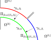
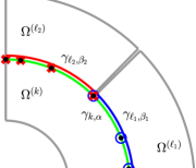
Figure 13: At left, interpolation from $\left(\gamma_{\ell_{1},\beta_{1}}\cup\gamma_{\ell_{2},\beta_{2}}\right)$ to $\gamma_{k,\alpha}$. Here ${\cal A}_{k,\alpha}=\{(\ell_{1},\beta_{1}),(\ell_{2},\beta_{2})\}$. At right, the black dots are the Greville nodes ${\bf x}_{i,G}^{(k,\alpha)}\in\gamma_{k,\alpha}$. The indices of the nodes surrounded by blue rings belong to ${\cal G}_{(k,\alpha)(\ell_{1},\beta_{1})}$, while the indices of the nodes marked with a red cross belong to ${\cal G}_{(k,\alpha)(\ell_{2},\beta_{2})}$ (see formula (124)). There is one Greville node that belongs to both the sets ${\cal G}_{(k,\alpha)(\ell_{1},\beta_{1})}$ and ${\cal G}_{(k,\alpha)(\ell_{2},\beta_{2})}$, the corresponding value $(U_{k,\alpha})_{i}$ is equal to 1/2. For all the other Greville nodes, $(U_{k,\alpha})_{i}$ is equal to 1

8.1 Extension of the interpolation matrices (51) and (52) for watertight interfaces.

We denote by ${\bf F}^{(k,\alpha)}:{\mathbb{R}}^{d-1}\to{\mathbb{R}}^{d}$ the restriction of ${\bf F}^{(k)}$ to the face $\widehat{\gamma}_{k,\alpha}=({\bf F}^{(k)})^{-1}(\gamma_{k,\alpha})$. Let ${\bf x}_{i,G}^{(k,\alpha)}$, for $i=1,\ldots,n^{(k,\alpha)}$, be the Greville nodes associated with the patch $\Omega^{(k)}$ that belong to $\gamma_{k,\alpha}$ and $\widehat{\bf x}_{i,G}^{(k,\alpha)}=({\bf F}^{(k,\alpha)})^{-1}({\bf x}_{i,G}^{(k,\alpha)})$ their counter-image in the face $\widehat{\gamma}_{k,\alpha}$ of the parameter domain. For any face $\gamma_{k,\alpha}$ and for any $(\ell,\beta)\in{\cal A}_{k,\alpha}$ we define the set

$${\cal G}_{(k,\alpha)(\ell,\beta)}=\{i=1,\ldots,n^{(k,\alpha)}|\ {\bf x}_{i,G}^{(k,\alpha)}\in\gamma_{\ell,\beta}\}$$ (124)

of the indices of the Greville nodes associated with the domain $\Omega^{(k)}$ belonging to $\gamma_{k,\alpha}$ that lay on $\gamma_{\ell,\beta}$ too (see Fig. 13, right).

Notice that ${\cal G}_{(k,\alpha)(\ell,\beta)}$ and ${\cal G}_{(\ell,\beta)(k,\alpha)}$ denote two different sets.

Finally, we define a sort of partition of unity function, with the aim of interpolating correctly the data coming from two contiguous faces adjacent to $\gamma_{k,\alpha}$.

For any $i=1,\ldots,n^{(k,\alpha)}$, we set

$$(U_{k,\alpha})_{i}=1/\mbox{card}\{(\ell,\beta)\in{\cal A}_{k,\alpha}|\ i\in{\cal G}_{(k,\alpha)(\ell,\beta)}\},$$ (125)

that is $(U_{k,\alpha})_{i}$ is the inverse of the number of faces adjacent to $\gamma_{k,\alpha}$ which the Greville node ${\bf x}_{i,G}^{(k,\alpha)}$ lays on (up to the boundary). Here, card$A$ denotes the cardinality of the set $A$.

Given $\lambda\in Y^{(\ell,\beta)}_{h_{\ell}}$ , we define the interpolation operator $\Pi_{(k,\alpha)(\ell,\beta)}:Y^{(\ell,\beta)}_{h_{\ell}}\to Y^{(k,\alpha)}_{h_{k}}$ by imposing the following interpolation conditions for $i=1,\ldots,n^{(k,\alpha)}$:

$$\begin{array}[]{lll}(\Pi_{(k,\alpha)(\ell,\beta)}\lambda)({\bf x}_{i,G}^{(k,\alpha)})=\left\{\begin{array}[]{ll}(U_{k,\alpha})_{i}\ \lambda({\bf x}_{i,G}^{(k,\alpha)})&\mbox{ if }i\in{\cal G}_{(k,\alpha)(\ell,\beta)},\\ 0&\mbox{ if }i\not\in{\cal G}_{(k,\alpha)(\ell,\beta)}\end{array}\right.\end{array}$$ (129)

Notice that $\Pi_{(k,\alpha)(\ell,\beta)}\lambda$ is defined on the whole face $\gamma_{k,\alpha}$, even when $\gamma_{\ell,\beta}\subsetneqq\gamma_{k,\alpha}$.

Let us consider the multipatch geometry shown in the top left picture of Fig. 14, we interpolate a trace function from $\gamma_{2,2}\cup\gamma_{3,2}$ to $\gamma_{1,1}$. In the bottom pictures of Fig. 14 we show how the interpolation operators $\Pi_{(1,1)(2,2)}$ (from $\gamma_{2,2}$ to $\gamma_{1,1}$) and $\Pi_{(1,1)(3,2)}$ (from $\gamma_{3,2}$ to $\gamma_{1,1}$) work. The point whose coordinates are $(x,y)=(1,1)$ is a Greville point for $\Omega^{(1)}$ belonging to $\gamma_{1,1}$ and it lays on both $\gamma_{2,2}$ and $\gamma_{3,2}$ too (the faces include their boundary), thus the corresponding weight defined in (125) is equal to 1/2. Notice that $(\Pi_{(1,1)(2,2)}\lambda)$ takes null value at the Greville nodes of $\gamma_{1,1}$ not laying on $\gamma_{2,2}$. Analogous considerations hold for $(\Pi_{(1,1)(3,2)}\lambda)$.

The sum $\Pi_{(1,1)(2,2)}\lambda^{(2,2)}+\Pi_{(1,1)(3,2)}\lambda^{(3,2)}$ interpolates the piece-wise function $\lambda$ such that $\lambda_{|\gamma_{2,2}}=\lambda^{(2,2)}$ and $\lambda_{|\gamma_{3,2}}=\lambda^{(3,2)}$ (see the right picture of Fig. 14).

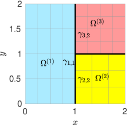
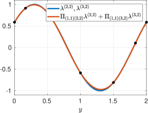
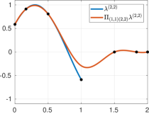
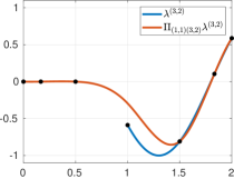
Figure 14: Example of how the interpolation operators $\Pi_{(k,\alpha)(\ell,\beta)}$ work. The black dots represent the interpolated values at the Greville nodes

Let $\mu_{j}^{(k,\alpha)}$, with $j=1,\ldots,n^{(k,\alpha)}$, be the NURBS basis functions of the trace space $Y_{h_{k}}^{(k,\alpha)}$ and $\mu_{j}^{(k,\alpha)}$ the corresponding basis function in the parameter domain, i.e. such that $\mu_{j}^{(k,\alpha)}=\widehat{\mu}_{j}^{(k,\alpha)}\circ({\bf F}^{(k,\alpha)})^{-1}$. By setting

$$\begin{array}[]{lll}(G_{(k,\alpha)(k,\alpha)})_{ij}&=\widehat{\mu}_{j}^{(k,\alpha)}(\widehat{\bf x}_{i,G}^{(k,\alpha)}),&i,j=1,\ldots,n^{(k,\alpha)},\\[5.69054pt] (G_{(k,\alpha)(\ell,\beta)})_{ij}&=\left\{\begin{array}[]{ll}\widehat{\mu}_{j}^{(\ell,\beta)}(({\bf F}^{(\ell,\beta)})^{-1}({\bf x}_{i,G}^{(k,\alpha)}))&\mbox{ if }i\in{\cal G}_{(k,\alpha)(\ell,\beta)}\\ 0&\mbox{ if }i\not\in{\cal G}_{(k,\alpha)(\ell,\beta)}\end{array}\right.,&i=1,\ldots,n^{(k,\alpha)},\ j=1,\ldots,n^{(\ell,\beta)}\end{array}$$ (134)

the matrix associated with $\Pi_{(k,\alpha)(\ell,\beta)}$ is

$$P_{(k,\alpha)(\ell,\beta)}=G_{(k,\alpha)(k,\alpha)}^{-1}\mbox{diag}(U_{k,\alpha})G_{(k,\alpha)(\ell,\beta)}.$$ (135)

Similarly, we define the interpolation operator $\Pi_{(\ell,\beta)(k,\alpha)}:Y^{(k,\alpha)}_{h_{k}}\to Y^{(\ell,\beta)}_{h_{\ell}}$ and the corresponding matrix

$$P_{(\ell,\beta)(k,\alpha)}=G_{(\ell,\beta)(\ell,\beta)}^{-1}\mbox{diag}(U_{\ell,\beta})G_{(\ell,\beta)(k,\alpha)}.$$ (136)

Denoting by $\boldsymbol{\lambda}_{k,\alpha}$ ($\boldsymbol{\lambda}_{\ell,\beta}$, resp.) the array whose entries are the degrees of freedom of the function $u^{(k)}_{h_{k}}$ ($u^{(\ell)}_{h_{\ell}}$, resp.) associated with the face $\gamma_{k,\alpha}$ ($\gamma_{\ell,\beta}$, resp.), the algebraic implementation of the interface conditions (123)₂ reads:

$$\begin{array}[]{ll}\mbox{for any }(\ell,\beta):\gamma_{\ell,\beta}\mbox{ is slave,}\displaystyle\qquad\boldsymbol{\lambda}_{\ell,\beta}=\sum_{(k,\alpha)\in{\cal A}_{\ell,\beta}}P_{(\ell,\beta),(k,\alpha)}\boldsymbol{\lambda}_{k,\alpha}.\end{array}$$ (138)

8.2 Transferring normal derivatives

For each face (either slave or master) $\gamma_{k,\alpha}\subset\Gamma_{k}=\partial\Omega^{(k)}\setminus\partial\Omega$, we define the set $G_{k,\alpha}=\partial\Omega^{(k)}\setminus\gamma_{k,\alpha}$ (or $G_{k,\alpha}=\partial\Omega^{(k)}\setminus(\gamma_{k,\alpha}\cup\partial\Omega^{(k)}_{N})$ when mixed boundary conditions are given on $\partial\Omega$) and the real values (similar to (63))

$$r^{(k,\alpha)}_{i}=\int_{\gamma_{k,\alpha}}\nu_{k}\frac{\partial u^{(k)}_{h_{k}}}{\partial{\bf n}_{k}}\,\overline{\cal L}^{(k)}\mu_{i}^{(k,\alpha)}\,d\Gamma,\quad i=1,\ldots,n^{(k,\alpha)}.$$ (139)

As done for the configuration with only two patches, we can compute $r^{(k,\alpha)}_{i}$ by exploiting the weak form of the differential equations inside the patches, i.e.

$$r^{(k,\alpha)}_{i}=a^{(k)}(u^{(k)}_{h_{k}},\overline{\cal L}^{(k)}\mu_{i}^{(k,\alpha)})-{\cal F}^{(k)}(\overline{\cal L}^{(k)}\mu_{i}^{(k,\alpha)})-\int_{G_{k,\alpha}}\nu_{k}\frac{\partial u^{(k)}_{h_{k}}}{\partial{\bf n}_{k}}\,\overline{\cal L}^{(k)}\mu_{i}^{(k,\alpha)}\,d\Gamma,\quad i=1,\ldots,n^{(k,\alpha)}.$$ (140)

Following the notations of Sect. 5, for any $k=1,\ldots,M$ and for any face $\gamma_{k,\alpha}\subset\Gamma_{k}$, we define the sets ${\cal I}_{\overline{\gamma}_{k,\alpha}}$, ${\cal I}_{\gamma_{k,\alpha}}$, and ${\cal I}_{\partial\gamma_{k,\alpha}}$. To evaluate the last integral of (140) we define the matrix $C^{(k,\alpha)}$ (of size $N^{(k)}\times N^{(k)}$) whose non-null entries are

$$\begin{array}[]{lll}C^{(k,\alpha)}_{ij}&\displaystyle=-\int_{G_{k,\alpha}}\nu_{k}\frac{\partial\varphi_{j}^{(k)}}{\partial{\bf n}_{k}}\varphi_{i}^{(k)},&\mbox{ for }i\in{\cal I}_{\partial\gamma_{k,\alpha}},\ j\in{\cal I}_{\overline{\Omega}^{(k)}}.\end{array}$$ (142)

Then we set

$$\widehat{A}^{(\overline{\gamma}_{k,\alpha},\overline{\Omega}^{(k)})}=A^{(\overline{\gamma}_{k,\alpha},\overline{\Omega}^{(k)})}+C^{(\overline{\gamma}_{k,\alpha},\overline{\Omega}^{(k)})}$$ (143)

and ${\bf f}_{k,\alpha}={\bf f}({\cal I}_{\overline{\gamma}_{k,\alpha}})$, and we compute

$${\bf r}_{k,\alpha}=\widehat{A}^{(\overline{\gamma}_{k,\alpha},\overline{\Omega}^{(k)})}{\bf u}^{(k)}-{\bf f}_{k,\alpha},$$

that will contain the values $r^{(k,\alpha)}_{i}$ defined in (140).

Finally, for any face $\gamma_{k,\alpha}$ we define the mass matrix

$$(M_{(k,\alpha)})_{ij}=(\mu_{j}^{(k)},\mu_{i}^{(k)})_{L^{2}(\gamma_{k,\alpha})},\qquad i,j=1,\ldots,n^{(k,\alpha)}.$$ (144)

The algebraic implementation of the interface conditions (123)₃ reads:

$$\begin{array}[]{ll}\mbox{for any }(k,\alpha):\gamma_{k,\alpha}\mbox{ is master,}\qquad\displaystyle{\bf r}_{k,\alpha}+\sum_{(\ell,\beta)\in{\cal A}_{k,\alpha}}M_{(k,\alpha)}P_{(k,\alpha),(\ell,\beta)}M_{(\ell,\beta)}^{-1}{\bf r}_{\ell,\beta}={\bf 0}.\end{array}$$ (146)

8.3 Comparison between INTERNODES and mortar methods

The mortar method is a well-established technology for the coupling of non-conforming discretizations. It suits also for problems where the non-conformities are intrinsic, such as the contact problems. Typically, in mortar methods the continuity between interfaces is imposed weakly, so that a procedure for integrating the product between basis functions of the master and those of the slave sides is required. In order to obtain optimal convergence rates, it is critical to define quadrature rules that compute very accurately, if not ever exactly, the cross mass matrix at the interface [5]. Adapting the quadrature points to the elements of the master side does not results in an optimal quadrature rule for the basis functions of the slave side, and vice-versa. A common strategy for overcoming this issue in the case of watertight interfaces consists in creating a third ”intersection mesh” between the master and slave meshes, in which the integration elements can be seen as belonging to both sides and thus the quadrature points defined over them allow for high accurate integration of both master and slave basis functions. Nevertheless, the generation of intersection meshes is far from trivial (from a theoretical and practical point of view) and may easily result in a number of elements that is of orders of magnitude greater than those of the two original meshes. Moreover, in the case of non-watertight interfaces the task acquires even greater complexity due to the need to project the quadrature nodes from one interface to the other.

On the contrary, INTERNODES requires local interface mass matrices involving only basis functions from one side of the interface (we refer to matrices (67)), and they can be assembled by taking into account only the parametrization of the relative patch.

Most often mortar methods are formulated as a saddle point problem by introducing an extra field, the Lagrange multiplier. This yields an inf-sup compatibility condition to be fulfilled in order to ensure well-posedness, and such condition affects the choice of the polynomial degrees of the NURBS spaces. [6]. On the contrary, INTERNODES does not introduce extra fields, so that it does not care of this problem and no constraints on the polynomial degrees are required.

When mortar methods are formulated as a single field problem (like (89)), the corresponding algebraic system is symmetric, provided the original differential operator is self-adjoint. This property is not fulfilled by INTERNODES due to the two a-priori different intergrid operators $\Pi_{12}$ and $\Pi_{21}$. Nevertheless, the local stiffness matrices continue to be symmetric and positive definite and we can solve the local differential subsystems by ad-hoc algebraic methods.

In [17, Sec. 6], the authors have compared both the eigenvalues and the iterative condition number of the matrix ${\mathbb{A}}$ with those of the analogous matrix built with mortar methods instead of INTERNODES. The eigenvalues of the mortar matrix are all real positive (since the global matrix results symmetric positive definite), whereas those of the INTERNODES matrix feature tiny imaginary parts that vanish as the step size does. Moreover the iterative condition number of the two matrices behaves right the same way. Since the eigenvalues of the Schur complement matrix are strictly connected with those of the original matrix, we conclude that also the eigenvalues of the corresponding Schur complement matrices behave similarly.

We notice that using only one intergrid interpolation operator (as, e.g., $\Pi_{21}$ jointly with its transpose $\Pi_{21}^{t}$) would not guarantee an accurate non-conforming method. The use of only one interpolation operator would yield the so-called pointwise matching discussed, e.g., in [3, 2].

About the accuracy, INTERNODES and mortar methods behaves exactly in the same way: the $H^{1}-$broken norm of the error decays optimally when the mesh-size tends to zero, i.e. the error produced by these two coupling methods is proportional to that of the discretization used inside the local subdomains and it depends on the regularity of the exact solution of the differential problem. The proof of this result for INTERNODES is under consideration in the IGA context, while in the Finite Element framework the theoretical analysis has been established in [21].

9 The iterative algorithm to solve (123).

We extend to each patch with index $k=1,\ldots,M$ the notations on the matrices and on the arrays introduced in Sect. 5 and we split the degrees of freedom (the unknown coefficients of each $u_{h_{k}}^{(k)}$ with respect to the NURBS basis functions) in:

1. ${\bf u}^{(k)}_{0}$: the degrees of freedom internal to $\Omega^{(k)}$,

2. ${\bf g}^{(k)}$: the degrees of freedom associated with the Dirichlet boundary $\partial\Omega^{(k)}_{D}$, if it is not empty,

3. ${\bf u}_{\Gamma}$: the (not replicated) degrees of freedom associated with the master skeleton $\Gamma$ defined in (117) deprived of the degrees of freedom associated with $\Gamma\cap\partial\Omega^{(k)}_{D}$.

Notice that only the degrees of freedom associated with the vertices of the patches are interpolatory and they are the only degrees of freedom which we must be careful to not replicate inside ${\bf u}_{\Gamma}$. In this way we automatically enforce the continuity of the solution at such interpolatory points.

For example, when we consider a decomposition like that sketched in Fig. 15, the vertex shared by all the four patches belongs to four master faces (the dark-gray ones), but only one occurrence of it must be considered in the array ${\bf u}_{\Gamma}$.

Notice that in the decompositions depicted in Fig. 11 the vertex of $\gamma_{3,1}$ (internal to $\Omega$) lays on the face $\gamma_{1,1}$, but it is not a degree of freedom for the patch $\Omega^{(1)}$ (the solely interpolation degrees of freedom of $\Omega^{(k)}$ are at the vertices of the patch itself).

If we eliminate the internal degrees of freedom ${\bf u}^{(k)}_{0}$, we obtain the Schur complement system with respect to ${\bf u}_{\Gamma}$:

$$S{\bf u}_{\Gamma}={\bf b}$$ (147)

and we can solve it by a Krylov method (e.g. Bi-CGStab, GMRES and so on), for which it is sufficient to provide an algorithm (see Algorithm 3) that, given an array $\boldsymbol{\lambda}$ of the same size of ${\bf u}_{\Gamma}$, computes $\boldsymbol{\psi}=S\boldsymbol{\lambda}$.

Since the array ${\bf u}_{\Gamma}$ does not contain the degrees of freedom associated with $\Gamma\cap\partial\Omega^{(k)}_{D}$, but at the same time the interpolation matrices work on the degrees of freedom associated with the faces up to their boundary, for practical purposes it is convenient to extend ${\bf u}_{\Gamma}$ to an array $\widetilde{\bf u}_{\Gamma}$ that includes also the null degrees of freedom associated with $\Gamma\cap\partial\Omega^{(k)}_{D}$.

We denote by $n_{\Gamma}$ the size of ${\bf u}_{\Gamma}$, by $\widetilde{n}_{\Gamma}$ the size of $\widetilde{\bf u}_{\Gamma}$ and we define the restriction matrix $R_{D}$ of size $\widetilde{n}_{\Gamma}\times n_{\Gamma}$ (whose entries are 0 or 1) that, with any array $\widetilde{\bf u}$ defined on $\Gamma$, associates its restriction to $\Gamma\setminus\partial\Omega$ such that ${\bf u}_{\Gamma}=R_{D}\widetilde{\bf u}_{\Gamma}$, and the prolongation (or extension-by-zero) matrix of size $n_{\Gamma}\times\widetilde{n}_{\Gamma}$ such that $\widetilde{\bf u}_{\Gamma}=R_{D}^{T}{\bf u}_{\Gamma}$.

Similarly, for any couple $(k,\alpha)$, we define the restriction matrix $R_{k,\alpha}$ of size $n^{(k,\alpha)}\times\widetilde{n}_{\Gamma}$ that implements the restriction of $\widetilde{\bf u}_{\Gamma}$ from $\Gamma$ to the degrees of freedom associated with $\gamma_{k,\alpha}$ (up to the boundary), i.e. ${\bf u}_{k,\alpha}=R_{k,\alpha}\widetilde{\bf u}_{\Gamma}$. Consequently, $R_{k,\alpha}^{T}$ implements the prolongation of ${\bf u}_{k,\alpha}$ to $\widetilde{\bf u}_{\Gamma}$.

In Fig. 15 and 16 we sketch a decomposition with 4 patches, we identify master (dark-gray) and slave (white) faces and we explain how the interpolation operators act.

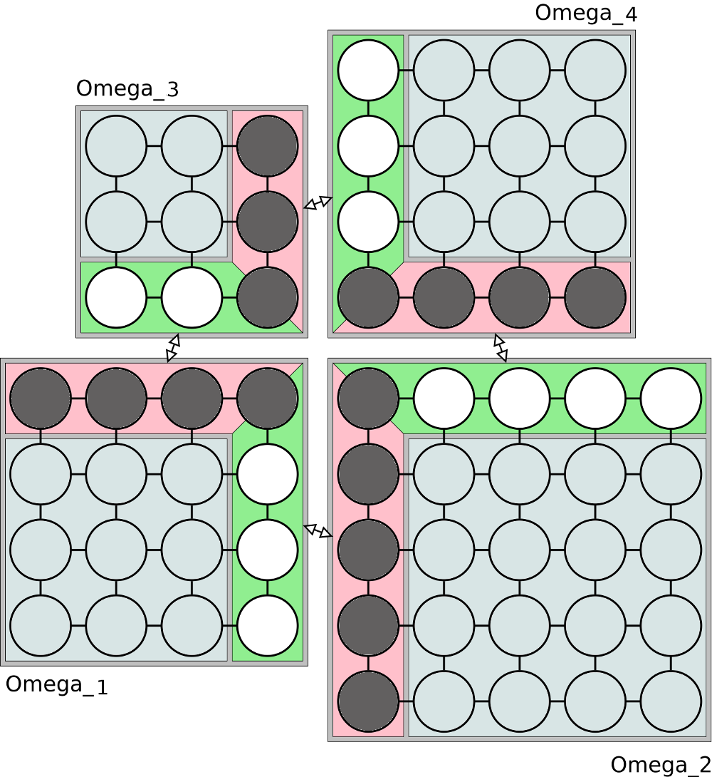
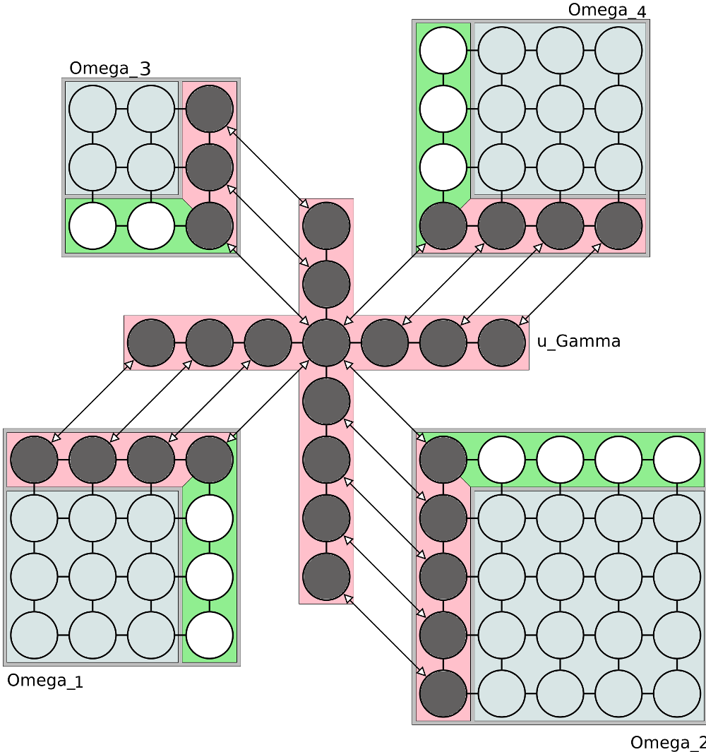
Figure 15: At left, the global layout for a situation with 4 patches, the circles denote the degrees of freedom. The dark-gray circles are those on the master faces, while the white ones are on the slave faces. At right, the degrees of freedom on the master skeleton and the correspondence between the master skeleton $\Gamma$ and the master faces $\gamma_{k,\alpha}$

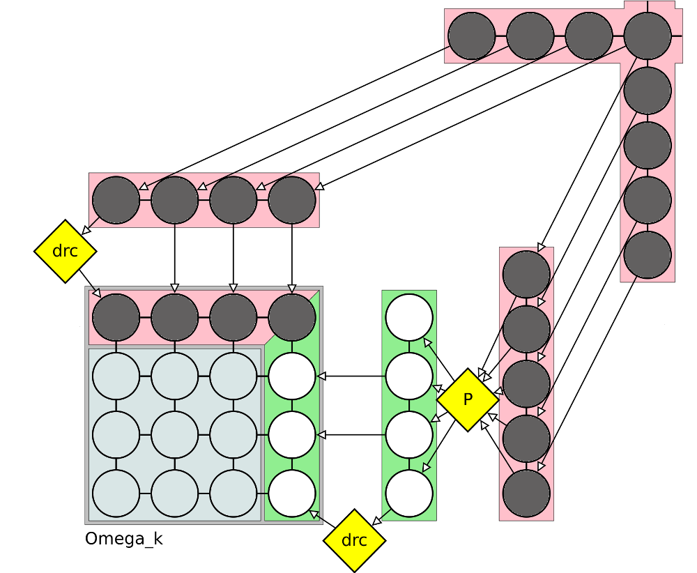
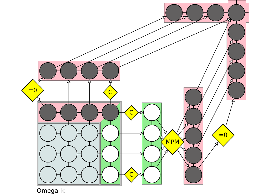
Figure 16: At left, the interpolation of the trace from the master faces to the slave faces, $P$ stands for the interpolation operator $\Pi_{(k,\alpha)(\ell,\beta)}$, “drc” stands for Dirichlet condition. At right, the interpolation of the normal derivatives from slave faces to master faces, $MPM$ stands for the interpolation operator $\widetilde{\Pi}_{(\ell,\beta)(k,\alpha)}$. “C” identifies the degrees of freedom on which the correction matrix $C^{(k)}$ defined in (142) acts

Algorithm 1 contains the instructions to initialize INTERNODES, Algorithm 2 computes the right hand side ${\bf b}$ of (147), while Algorithm 3 implements the matrix vector product $\boldsymbol{\psi}=S\boldsymbol{\lambda}$ that can be used at each iteration of the iterative method called to solve (147). Once that ${\bf u}_{\Gamma}$ has been computed, we can recover the solution ${\bf u}^{(k)}$ in every patch by applying Algorithm 4.

for all patch $k=1,\ldots,M$ do

     build the local stiffness matrices $A^{(k)}$ 

     build the arrays ${\bf f}^{(k)}$, ${\bf g}_{k}$, ${\bf g}_{\partial\Gamma_{k}}$ 

     build the matrices $C^{(k)}$ (see (142)) and $\widehat{A}^{(\overline{\gamma}_{k,\alpha},\overline{\Omega}^{(k)})}$ (see (143))  

     build the Greville nodes in $\Omega^{(k)}$ 

     for all face $\alpha$ of $\Gamma_{k}$ do

         build the local interface mass matrices $M_{(k,\alpha)}$ (formula (144)) 

         for all face $(\ell,\beta)\in{\cal A}_{(k,\alpha)}$ do

              build the interpolation matrices $P_{(k,\alpha)(\ell,\beta)}$ (either formulas (135) or (61)–(62)) 

         end for

     end for

end for

Algorithm 1 Initialization of INTERNODES

% Distribute the Dirichlet dof

for all patch $k=1,\ldots,M$ do

     ${\bf t}^{(k)}={\bf 0}$ (array of the dof associated with $\partial\Omega^{(k)}$) 

     ${\bf t}^{(k)}|_{\partial\Omega_{D}^{(k)}}={\bf g}|_{\partial\Omega_{D}^{(k)}}$ 

end for

% Interpolate from master faces to slave faces

for all patch $\ell=1,\ldots,M$ do

     for all slave face $\beta$ of $\Gamma_{\ell}$ do

         $\displaystyle{\bf t}^{(\ell)}|_{(\ell,\beta)}=\sum_{(k,\alpha)\in{\cal A}_{(\ell,\beta)}}P_{(\ell,\beta)(k,\alpha)}{\bf t}^{(k)}|_{(k,\alpha)}$ 

     end for

end for

% Solve local independent subproblems and compute ${\bf r}_{k,\alpha}$ face by face

for all patch $k=1,\ldots,M$ do

     solve $A^{(k,k)}{\bf u}^{(k)}_{0}={\bf f}^{(k)}_{0}-A^{(k,\partial\Omega^{(k)})}{\bf t}^{(k)}$ 

     assemble ${\bf u}^{(k)}=[{\bf u}^{(k)}_{0},{\bf t}^{(k)}]$ 

     for all face $\alpha$ of $\Gamma_{k}$ do

         ${\bf r}_{k,\alpha}=\widehat{A}^{(\overline{\gamma}_{k,\alpha},\overline{\Omega}^{(k)})}{\bf u}^{(k)}-{\bf f}_{k,\alpha}$ 

     end for

end for

% Interpolate the derivatives from slave to master faces and assemble from local faces to global master skeleton

$\widetilde{\bf b}={\bf 0}$  

for all patch $k=1,\ldots,M$ do

     for all master face $\alpha$ of $\Gamma_{k}$ do

         $\widetilde{\bf b}=\widetilde{\bf b}+R_{(k,\alpha)}^{T}\left(\displaystyle{\bf r}_{k,\alpha}+\sum_{(\ell,\beta)\in{\cal A}_{(k,\alpha)}}M_{(k,\alpha)}P_{(k,\alpha)(\ell,\beta)}M_{(\ell,\beta)}^{-1}{\bf r}_{\ell,\beta}\right)$ 

     end for

end for

% Restrict $\widetilde{\bf b}$ to $\Gamma\setminus\partial\Omega$

${\bf b}=R_{D}\widetilde{\bf b}$ 

Algorithm 2 Computation of the right hand side ${\bf b}$ of (147)

% Expand $\boldsymbol{\lambda}$ from $\Gamma\setminus\partial\Omega$ to $\Gamma$ 

$\widetilde{\boldsymbol{\lambda}}=R_{D}^{T}\boldsymbol{\lambda}$  

% Distribute the trace from the global master skeleton $\Gamma$ to the local master faces

for all patch $k=1,\ldots,M$ do

     ${\bf t}^{(k)}={\bf 0}$ (array of the dof associated with $\partial\Omega^{(k)}$) 

     for all master face $\alpha$ of $\Gamma_{k}$ do

         ${\bf t}^{(k)}|_{(k,\alpha)}=R_{(k,\alpha)}\widetilde{\boldsymbol{\lambda}}$ 

     end for

end for

% Interpolate from master faces to slave faces

for all patch $\ell=1,\ldots,M$ do

     for all slave face $\beta$ of $\Gamma_{\ell}$ do

         $\displaystyle{\bf t}^{(\ell)}|_{(\ell,\beta)}=\sum_{(k,\alpha)\in{\cal A}_{(\ell,\beta)}}P_{(\ell,\beta)(k,\alpha)}{\bf t}^{(k)}|_{(k,\alpha)}$ 

     end for

end for

% Solve local independent subproblems and compute ${\bf r}_{k,\alpha}$ face by face

for all patch $k=1,\ldots,M$ do

     solve $A^{(k,k)}{\bf u}^{(k)}_{0}=-A^{(k,\partial\Omega^{(k)})}{\bf t}^{(k)}$ 

     assemble ${\bf u}^{(k)}=[{\bf u}^{(k)}_{0},{\bf t}^{(k)}]$ 

     for all face $\alpha$ of $\Gamma_{k}$ do

         compute ${\bf r}_{k,\alpha}=\widehat{A}^{(\overline{\gamma}_{k,\alpha},\overline{\Omega}^{(k)})}{\bf u}^{(k)}$ 

     end for

end for

$\widetilde{\boldsymbol{\psi}}={\bf 0}$ (same size as $\widetilde{\boldsymbol{\lambda}}$) 

% Interpolate the derivatives from slave to master faces and assemble from local faces to global master skeleton

for all patch $k=1,\ldots,M$ do

     for all master face $\alpha$ of $\Gamma_{k}$ do

         $\widetilde{\boldsymbol{\psi}}=\widetilde{\boldsymbol{\psi}}+R_{(k,\alpha)}^{T}\left(\displaystyle{\bf r}_{k,\alpha}+\sum_{(\ell,\beta)\in{\cal A}_{(k,\alpha)}}M_{(k,\alpha)}P_{(k,\alpha)(\ell,\beta)}M_{(\ell,\beta)}^{-1}{\bf r}_{\ell,\beta}\right)$ 

     end for

end for

% Restrict $\boldsymbol{\psi}$ to $\Gamma\setminus\partial\Omega$

$\boldsymbol{\psi}=R_{D}\widetilde{\boldsymbol{\psi}}$ 

Algorithm 3 Given $\boldsymbol{\lambda}$, computation of $\boldsymbol{\psi}=S\boldsymbol{\lambda}$. This is the matrix-vector product needed to solve (147) by Krylov methods

% Expand ${\bf u}_{\Gamma}$ from $\Gamma\setminus\partial\Omega$ to $\Gamma$ 

$\widetilde{\bf u}_{\Gamma}=R_{D}^{T}{\bf u}_{\Gamma}$  

% Distribute the Dirichlet dof and the trace from $\Gamma$ to the master faces $\gamma_{k,\alpha}$

for all patch $k=1,\ldots,M$ do

     ${\bf t}^{(k)}={\bf 0}$ (array of the dof associated with $\partial\Omega^{(k)}$) 

     for all master face $\alpha$ of $\Gamma_{k}$ do

         ${\bf t}^{(k)}|_{(k,\alpha)}=R_{(k,\alpha)}\widetilde{\bf u}_{\Gamma}$ 

     end for

     ${\bf t}^{(k)}|_{\partial\Omega_{D}^{(k)}}={\bf g}|_{\partial\Omega_{D}^{(k)}}$ 

end for

% Interpolate from master faces to slave faces

for all patch $\ell=1,\ldots,M$ do

     for all slave face $\beta$ of $\Gamma_{\ell}$ do

         $\displaystyle{\bf t}^{(\ell)}|_{(\ell,\beta)}=\sum_{(k,\alpha)\in{\cal A}_{(\ell,\beta)}}P_{(\ell,\beta)(k,\alpha)}{\bf t}^{(k)}|_{(k,\alpha)}$ 

     end for

end for

% Solve local independent subproblems

for all patch $k=1,\ldots,M$ do

     solve $A^{(k,k)}{\bf u}^{(k)}_{0}={\bf f}^{(k)}_{0}-A^{(k,\partial\Omega^{(k)})}{\bf t}^{(k)}$ 

     assemble ${\bf u}^{(k)}=[{\bf u}^{(k)}_{0},{\bf t}^{(k)}]$ 

end for

Algorithm 4 Given ${\bf u}_{\Gamma}$, computation of the local solutions ${\bf u}^{(k)}$, for $k=1,\ldots,M$

10 Numerical results for $M>2$ patches

10.1 Test case #3

In this test case we consider watertight interfaces, but with non-matching parametrizations. Let us consider again the differential problem (3) in $\Omega=\{(x,y)\in{\mathbb{R}}^{2}:\ x\geq 0,\ y\geq 0,\ 1\leq x^{2}+y^{2}\leq 4\}$ with $\alpha=0$, and $f$ and $g$ such that the exact solution is $u(x,y)=\sin(1.5\pi x)\sin(3\pi y)$. Now we split $\Omega$ in 7 patches and we tag the master/slave interfaces as shown in the left picture of Fig. 17. We fix the polynomial degree equal to $p=2,\ldots,5$ in all the patches, while the number of elements inside the patches is defined as in the following table, with $\overline{n}=4,8,16,32$:

patch	number of elements
$\Omega^{(1)}$	$(\overline{n}+2)\times\overline{n}$
$\Omega^{(2)}$ and $\Omega^{(5)}$	$\overline{n}\times\overline{n}$
$\Omega^{(3)}$ and $\Omega^{(4)}$	$(\overline{n}+1)\times(\overline{n}+1)$
$\Omega^{(6)}$	$\overline{n}\times 3\overline{n}$
$\Omega^{(7)}$	$(\overline{n}+2)\times\overline{n}$

As in the Test case #1, the first parametric coordinate is mapped onto the radial coordinate of the physical domain, and the second coordinate onto the angular one. The patches are sectors of rings, the control points are defined as described in [9, Sect. 2.4.1.1], in particular the patches $\Omega^{(k)}$ with $k=1,\ldots,5$ have $30^{\circ}$ degrees arcs, while $\Omega^{(6)}$ and $\Omega^{(7)}$ have $45^{\circ}$ degrees arcs. Once the control points and the weights have been computed, the NURBS parametrization of the patches is defined as in (32). In the right picture of Fig. 17 the broken-norm errors (104) are shown versus $h=\max_{k}h_{k}$ for $p=2,\ldots,5$. As in the case of two subdomains, INTERNODES exhibits optimal convergence order with respect to the mesh size $h$.

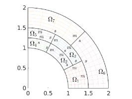
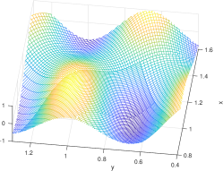
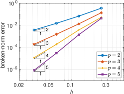
Figure 17: Test case #3. At left, the multipatch configuration; in the middle, a zoom on the numerical solution computed with $p=4$ and $\overline{n}=8$; at right, the broken-norm error versus the mesh size $h=\max_{k}h_{k}$

10.2 Test case #4. Jumping coefficients, the Kellogg’s test case

We solve the elliptic problem $-\nabla\cdot(\nu\nabla u)=0$ in $\Omega=(-1,1)^{2}$ with Dirichlet boundary conditions on $\partial\Omega$ and piece-wise constant coefficient $\nu$ such that the exact solution is the so-called Kellogg’s function (see, e.g., [36, 24, 22]). This is a very challenging problem whose solution features low regularity. We refer to [31] for a more in-depth analysis of the problem in the framework of isogeometric analysis.

The Kellogg’s solution can be written in terms of the polar coordinates $r$ and $\theta$ as $u(r,\theta)=r^{\gamma}\mu(\theta)$, where $\gamma\in(0,2)$ is a given parameter, while $\mu(\theta)$ is a $2\pi-$periodic continuous function defined like follows:

$$\mu(\theta)=\left\{\begin{array}[]{ll}\cos((\pi/2-\sigma)\gamma)\cos((\theta-\pi/2+\rho)\gamma)&0\leq\theta\leq\pi/2\\ \cos(\rho\gamma)\cos((\theta-\pi+\sigma)\gamma)&\pi/2\leq\theta\leq\pi\\ \cos(\sigma\gamma)\cos((\theta-\pi-\rho)\gamma)&\pi\leq\theta\leq 3\pi/2\\ \cos((\pi/2-\rho)\gamma)\cos((\theta-3\pi/2-\sigma)\gamma)&3\pi/2\leq\theta\leq 2\pi.\end{array}\right.$$ (152)

The parameters $\sigma$, $\rho$, $\gamma$ and the coefficient $R$ (that is involved in the definition of $\alpha$) must satisfy the following non-linear system:

$$\left\{\begin{array}[]{l}R=-\tan((\pi/2-\sigma)\gamma)\cot(\rho\gamma)\\ \frac{1}{R}=-\tan(\rho\gamma)\cot(\sigma\gamma)\\ R=-\tan(\sigma\gamma)\cot((\pi/2-\rho)\gamma)\\ 0<\gamma<2\\ \max\{0,\pi\gamma-\pi\}<2\gamma\rho<\min\{\gamma\pi,\pi\}\\ \max\{0,\pi-\gamma\pi\}<-2\gamma\sigma<\min\{\pi,2\pi-\gamma\pi\}.\end{array}\right.$$ (159)

We set $\nu=R>0$ in the first and the third quadrants, and $\nu=1$ in the second and in the fourth ones.

The case $\gamma=1$ is trivial since the solution is a plane. When $\gamma\neq 1$, then $u\in H^{1+\gamma-\varepsilon}(\Omega)$ for any $\varepsilon>0$, in particular the solution features low regularity at the origin and on the axes.

We look for the approximation of the Kellogg’s solution by applying INTERNODES to the 4-subdomains decomposition induced by the discontinuity of $\nu$.

For $\bar{n}\in\{5,10,\ldots,30\}$ we consider $(2\bar{n}+1)\times(2\bar{n}+1)$ equal elements in both $\Omega^{(1)}$ and $\Omega^{(3)}$ and $(\bar{n}-1)\times(\bar{n}-1)$ equal elements in both $\Omega^{(2)}$ and $\Omega^{(4)}$, so that the parametrizations (defined as in (32) do not match on any couple of interfaces. To analyze the errors we take the same polynomial degree $p$ along each direction and in all patches.

In the left picture of Fig. 18 the multipatch configuration is shown; in the middle picture of the same Figure the numerical solution corresponding to $\gamma=0.6$ is plotted, it is computed by setting the polynomial degree $p=2$ in each patch, $11\times 11$ equal elements in $\Omega^{(1)}$ and $\Omega^{(3)}$ and $4\times 4$ equal elements in both $\Omega^{(2)}$ and $\Omega^{(4)}$.

We have considered four different values of $\gamma$:

1. $\gamma=0.1$ and $R\simeq 161.45$, so that the corresponding Kellogg’s solution $u$ belongs to $H^{1.1-\varepsilon}(\Omega)$ (for any $\varepsilon>0$),

2. $\gamma=0.4$ and $R\simeq 9.47$, they provide $u\in H^{1.4-\varepsilon}(\Omega)$,

3. $\gamma=0.6$ and $R\simeq 3.85$, they provide $u\in H^{1.6-\varepsilon}(\Omega)$,

4. $\gamma=1.8$ and $R\simeq 2.5\cdot 10^{-2}$, they provide $u\in H^{2.8-\varepsilon}(\Omega)$.

The broken-norm errors (104) versus the mesh size $h=\max_{k}h_{k}$ are shown in the right picture of Fig. 18. They behave like $h^{\min(s-1,p)}$ when $h\to 0$, where $s=1+\gamma-\varepsilon$ is the Sobolev regularity of the Kellogg’s solution. We conclude that the INTERNODES solution is converging to the exact one when $h\to 0$ with the best possible convergence rate dictated by the regularity of the Kellogg’s solution.

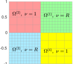
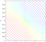
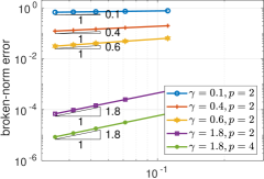
Figure 18: Test case #4. Kellogg’s solution. At left, the geometry for the Kellogg’s test case. At middle, the numerical solution with $\gamma=0.6$. At right the errors versus the discretization parameter $h_{1}=1/n_{el}^{(1)}$

We briefly comment on the algebraic solution of the Schur complement system (97). The number of Bi-CGStab iterations needed to solve (97) depends on the regularity of the solution (dictated by the parameter $\gamma$), on the mesh-sizes $h_{k}$, on the polynomial degrees $p$, and on the choice of the master/slave edges. In Table 2, left, we show the number #it of Bi-CGStab iterations needed to converge up a tolerance $\epsilon=10^{-10}$ for three different configurations of master/slave interfaces, for $\gamma\in\{0.6,\ 1.8\}$, and for some values of $h_{k}$ and $p$. The master/slave configuration that performs better is that featuring all the master edges inside the patches with the coarser meshes (i.e. $\Omega^{(2)}$ and $\Omega^{(4)}$). The dependence of #it on $p$ reflects the way the condition numbers of stiffness IGA matrices depend on $p$.

In the case that we can distinguish between master and slave patches (we say that a patch is master (slave resp.) if all its edges are tagged as master (slave, resp.)), to reduce the number of iterations we implement a preconditioner $P$ as follows (it is a generalization of the Dirichlet/Neumann preconditioner for substructuring domain decomposition methods [40]). We denote by $R_{\Gamma_{k}}$ the restriction matrix from the global master skeleton $\Gamma$ to the internal boundary $\Gamma_{k}$ of $\Omega^{(k)}$ and by $U$ a diagonal matrix whose element $U_{ii}$ is the number of master patches which the $i$th degree of freedom of $\Gamma$ belongs to. Then we define $P$ such that:

$$P^{-1}=U^{-1}\sum_{\tiny\begin{array}[]{c}k\\ master\end{array}}R^{T}_{\Gamma_{k}}S_{\Gamma_{k}}^{-1}R_{\Gamma_{k}}.$$ (160)

The matrices $S_{\Gamma_{k}}^{-1}$ are never built explicitly; to compute $S_{\Gamma_{k}}^{-1}{\bf v}$ we must solve a differential problem in $\Omega^{(k)}$ of the same nature of (3), but with Neumann (instead of Dirichlet) data on $\Gamma_{k}$ (see [40]).

The PBi-CGStab iterations with $P$ defined as in (160) are shown in Table 2, right, they are independent of the discretization parameters $h$ and $p$, but they depend on both the master/slave configuration and the regularity of the Kellogg’s solution.

A more in-depth analysis of suitable preconditioners for system (97) will be subject of future work.

	$\gamma=0.6$			$\gamma=1.8$			$\gamma=1.8$
	$p=2$			$p=2$			$p=4$
$\overline{n}$	(a)	(b)	(c)	(a)	(b)	(c)	(a)	(b)	(c)
10	17	12	16	43	13	42	86	23	79
15	21	14	19	47	15	44	103	25	97
20	25	17	22	56	17	54	118	23	99
25	30	18	25	62	20	51	115	25	105
30	33	22	28	61	22	52	110	27	124

	$\gamma=0.6$		$\gamma=1.8$		$\gamma=1.8$
	$p=2$		$p=2$		$p=4$
$\overline{n}$	(a)	(b)	(a)	(b)	(a)	(b)
10	7	10	21	5	21	5
15	8	11	21	5	24	5
20	7	11	23	5	22	5
25	9	11	23	5	23	5
30	9	11	21	5	25	5

Table 2: Test case # 4. At left, the number of Bi-CGStab iterations needed to solve (97). (a) $\Omega^{(1)}$ and $\Omega^{(3)}$ master patches; (b) $\Omega^{(2)}$ and $\Omega^{(4)}$ master patches; (c) one master edge and one slave edge for each patch. At right, number of PBi-CGStab iterations needed to solve (97). The preconditioner $P$ is defined in (160)

Finally, in Table 3 the number of PBi-CGStab iterations required to solve the Schur complement system (97) is shown for all the considered values of $\gamma$, here we have tagged as master the interfaces of the patches $\Omega^{(2)}$ and $\Omega^{(4)}$ and slave the others.

$\overline{n}$	dof$(\Omega)$		$\gamma=0.1$	$\gamma=0.4$	$\gamma=0.6$	$\gamma=1.8$
	$p=2$	$p=4$	$p=2$	$p=2$	$p=2$	$p=2$	$p=4$
$10$	1300	1588	11	10	10	5	5
$15$	2690	3098	11	11	11	5	5
$20$	4580	5108	12	12	11	5	5
$25$	6970	7618	12	11	11	5	5
$30$	9860	10628	12	11	11	5	5

Table 3: Test case #4. Comparison of the number of PBi-CGStab iterations required to solve the Schur complement system (97) for all the values of $\gamma$ considered in Fig. 18. $\Omega^{(2)}$ and $\Omega^{(4)}$ master patches

Remark 10.1

The preconditioner defined in (160) can be extended to more general decompositions provided that all the interfaces of a single patch can be tagged either slave or master. Moreover, in the case that a patch has empty intersection with $\partial\Omega$ and the corresponding local Schur complement is singular, the strategy to add the mass matrix to the stiffness one can be adopted (see, e.g., [40]). The design of suitable preconditioners for more general configurations with both master and slave edges in a single patch requires further work.

10.3 Test case #5. Non-watertight interfaces

We solve the elliptic problem $-\nabla\cdot(\nu\nabla u)+u=0$ in $\Omega=(0,3)^{2}$ with homogeneous Dirichlet boundary conditions on $\partial\Omega$ and piece-wise constant coefficient $\nu$. The computational domain is split into nine patches as shown in Fig. 19. The interfaces are non-watertight and they are obtained by B-spline interpolation of sinusoidal curves, as already described in Sect. 6.2. The maximum size of gaps and overlaps has been set $d_{\Gamma}\simeq 0.0276$.

Then we define a piecewise function $\nu$ that assumes the values $\{10,0.005,1,0.01,100,0.005,1,.005,0.1\}$ inside the patches (ordered as in the left picture of Fig. 19) (when two patches overlap we consider two different values of $\nu$, depending on the patch (see, e.g., [28])).

We have considered uniform knot sets in all the patches, the number of elements can be read from the left picture of Fig. 19. The numerical solution, computed with INTERNODES and RL-RBF interpolation is shown in Fig. 19, right.

The interfaces of the odd patches have been tagged as master, those of the even patches as slave and we have solved the Schur complement system (97) by the preconditioned Bi-CGStab iterations, with preconditioner $P$ build as mentioned for the Test case #4. 25 iterations have been required by the PBi-CGStab method to converge up to a tolerance of $\epsilon=10^{-10}$.

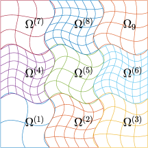
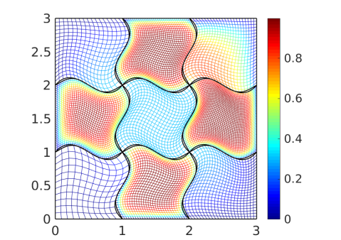
Figure 19: Test case #5. At left, the geometry; at right the numerical solution computed by INTERNODES and RL-RBF. The number of grid points used in the right plot is about twice the number of degrees of freedom

10.4 Test case #6. $C^{\infty}-$ solution on a 3D geometry

Let us consider the differential problem (3) with $\alpha=1$ in the domain $\Omega=\{(x,y,z)\in{\mathbb{R}}^{3}:\ 0.25\leq(x^{2}+y^{2})\leq 2.25,\ 0\leq z\leq 1\}$. The functions $f$ and $g$ are such that the exact solution is $u(x,y,z)=\sin(\pi x)\sin(\pi y)\cos(2\pi z)$.

The domain $\Omega$ is split into four patches like in Fig. 12 featuring non-matching NURBS parametrizations at the interfaces, even if they are watertight. More precisely, in cylindrical coordinates the patches are $\Omega^{(1)}=\{(r,\theta,z):\ 0.5\leq r\leq 1,\ 0\leq\theta\leq\pi/2,\ 0\leq z\leq 1\}$, $\Omega^{(2)}=\{(r,\theta,z):\ 1\leq r\leq 1.5,\ 0\leq\theta\leq\pi/2,\ 0\leq z\leq 0.5\}$, $\Omega^{(3)}=\{(r,\theta,z):\ 1\leq r\leq 1.5,\ 0\leq\theta\leq\pi/4,\ 0.5\leq z\leq 1\}$, $\Omega^{(4)}=\{(r,\theta,z):\ 1\leq r\leq 1.5,\ \pi/4\leq\theta\leq\pi/2,\ 0.5\leq z\leq 1\}$. The control points and the weights of the sector of rings are defined accordingly to [9, Sect. 2.4], then the $xy-$surfaces have been extruded along the $z$ direction.

The master skeleton is $\Gamma=\gamma_{1,1}\cup\gamma_{3,1}\cup\gamma_{3,3}\cup\gamma_{4,3}$ (see the caption of Fig. 20 for the numbering of the faces).

For $\overline{n}=2,\ldots,8$ we have considered $\overline{n}\times\overline{n}\times\overline{n}$ equal elements in both $\Omega^{(1)}$ and $\Omega^{(4)}$, and $(\overline{n}+1)\times(\overline{n}+1)\times(\overline{n}+1)$ equal elements in both $\Omega^{(2)}$ and $\Omega^{(3)}$. The discretizations on the two sides of any interface are totally unrelated.

To analyze the behaviour of the broken-norm error with respect to the mesh size, we have considered the same polynomial degree $p$ along each parametric direction and in all patches.

In the left picture of Fig. 20 we show the broken-norm error (104) versus the mesh size $h=\max_{k}h_{k}$. We observe that $\|u-u_{h}\|_{*}\simeq{\cal O}(h^{p})$ when $h\to 0$ and we conclude that the INTERNODES solution is converging to the exact one when $h\to 0$ with the best possible convergence rate dictated by the NURBS-discretization inside the patches (see, e.g., [13, Thm. 3.4 and Cor. 4.16]). In the right picture of Fig. 20 the numerical solution computed with $p^{(1)}=p^{(3)}=4$, $p^{(2)}=p^{(4)}=3$, $3\times 3\times 3$ elements in both $\Omega^{(1)}$ and $\Omega^{(4)}$ and $4\times 4\times 4$ elements in both $\Omega^{(2)}$ and $\Omega^{(3)}$ is shown.

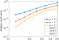
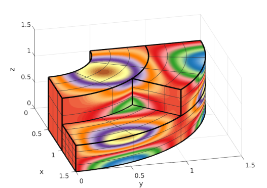
Figure 20: Test case #6. At left, the broken-norm errors versus the discretization parameter $h$, $p$ is the same in all patches. At right, the plot of the numerical solution in the patches $\Omega^{(1)}\cup\Omega^{(2)}\cup\Omega^{(4)}$, computed with: $p^{(1)}=p^{(3)}=4$, $p^{(2)}=p^{(4)}=3$, $3\times 3\times 3$ elements in both $\Omega^{(1)}$ and $\Omega^{(4)}$ and $4\times 4\times 4$ elements in both $\Omega^{(2)}$ and $\Omega^{(3)}$. We have removed the patch $\Omega^{(3)}$ to have a look on the solution inside $\Omega$

10.5 Test case #7. 3D re-entrant corner

Let us consider the differential problem (3) in a non-convex domain with a re-entrant corner, as shown in Fig. 21, more precisely $\Omega=\{(x,y,z)\in{\mathbb{R}}^{3}:(x+0.5)^{2}+(y+0.5)^{2}\leq 4,\ x\geq-0.5,\ y\geq-0.5,\ 0\leq z\leq 1\}\setminus([-0.5,0)\times[-0.5,0)\times[0,1])$. Then we set $\alpha=0$ , and $f$ and $g$ such that the exact solution in cylindrical coordinates reads $u(r,\theta,z)=r^{\beta}\sin(\beta\theta)\sin(\beta z)$, with $\beta>0$. The solution features low regularity in a neighborhood of the $z-$axis, in particular it holds $u\in H^{1+\beta}(\Omega)$.

The computational domain $\Omega$ is split into four patches as shown in Fig. 21, all the interfaces are watertight, but with non-matching parametrizations: for $\overline{n}=2,\ldots,6$ we have discretized the patches as follows: $\overline{n}\times 3\overline{n}\times\overline{n}$ elements in $\Omega^{(1)}$, $3\overline{n}\times\overline{n}\times\overline{n}$ elements in $\Omega^{(2)}$, $\overline{n}\times(\overline{n}+2)\times\overline{n}$ elements in $\Omega^{(3)}$, and $\overline{n}\times(\overline{n}+1)\times\overline{n}$ elements in $\Omega^{(4)}$. The first, second, and third parametric coordinates are mapped onto the radial, the angular, and the vertical physical coordinates, respectively.

In the right picture of Fig. 21 we show the broken-norm errors for $\beta=2/3$, $\beta=5/3$ and $\beta=7/3$ for the INTERNODES solution, that is converging to the exact one when $h\to 0$ with the best possible convergence rate dictated by the regularity of the test solution.

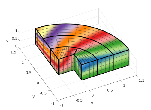
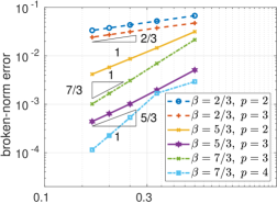
Figure 21: Test case #7. At left, the multipatch configuration. At right, the broken-norm errors versus the discretization parameter $h$, for three values of $\beta$. The polynomial degree $p$ is the same in all patches

References

- [1] F. Auricchio, L. Beirão da Veiga, T.J.R. Hughes, A. Reali, and G. Sangalli. Isogeometric collocation methods. Math. Models Methods Appl. Sci., 20(11):2075–2107, 2010.
- [2] C. Bègue, C. Bernardi, N. Debit, Y. Maday, G.E. Karniadakis, C. Mavriplis, and A.T. Patera. Nonconforming spectral element-finite element approximations for partial differential equations. In Proceedings of the Eighth International Conference on Computing Methods in Applied Sciences and Engineering, volume 75, pages 109–125, 1989.
- [3] C. Bernardi, Y. Maday, and A.T. Patera. A new nonconforming approach to domain decomposition: the mortar element method. In Nonlinear partial differential equations and their applications. Collège de France Seminar, Vol. XI (Paris, 1989–1991), volume 299 of Pitman Res. Notes Math. Ser., pages 13–51. Longman Sci. Tech., Harlow, 1994.
- [4] H. J. Brauchli and J. T. Oden. Conjugate approximation functions in finite-element analysis. Quart. Appl. Math., 29:65–90, 1971.
- [5] E. Brivadis, A. Buffa, B. Wohlmuth, and L. Wunderlich. The influence of quadrature errors on isogeometric mortar methods. In Isogeometric analysis and applications 2014, volume 107 of Lect. Notes Comput. Sci. Eng., pages 33–50. Springer, Cham, 2015.
- [6] E. Brivadis, A. Buffa, B. Wohlmuth, and L. Wunderlich. Isogeometric mortar methods. Computer Methods in Applied Mechanics and Engineering, 284:292–319, 2015.
- [7] C.L. Chan, C. Anitescu, and T. Rabczuk. Isogeometric analysis with strong multipatch c1-coupling. Computer Aided Geometric Design, 62:294–310, 2018.
- [8] L. Coox, F. Greco, O. Atak, D. Vandepitte, and W. Desmet. A robust patch coupling method for nurbs-based isogeometric analysis of non-conforming multipatch surfaces. Computer Methods in Applied Mechanics and Engineering, 316:235–260, 2017.
- [9] J.A. Cottrell, T.J.R. Hughes, and Y. Bazilevs. Isogeometric Analysis: Toward Integration of CAD and FEA. Wiley, 2009.
- [10] J.A. Cottrell, T.J.R. Hughes, and A. Reali. Studies of refinement and continuity in Isogeometric structural analysis. Comput. Methods Appl. Mech. Engrg., 196:4160–4183, 2007.
- [11] L. Beirão da Veiga, A. Buffa, D. Cho, and G. Sangalli. IsoGeometric analysis using T-splines on two-patch geometries. Computer Methods in Applied Mechanics and Engineering, 200(21-22):1787–1803, 2011.
- [12] L. Beirão da Veiga, A. Buffa, G. Sangalli, and R. Vàzquez. Mathematical analysis of variational isogeometric methods. Acta Numerica, 23:157–287, 2014.
- [13] L. Beirão da Veiga, A. Buffa, G. Sangalli, and R. Vàzquez. An introduction to the numerical analysis of isogeometric methods. In Numerical simulation in physics and engineering, volume 9 of SEMA SIMAI Springer Ser., pages 3–69. Springer, 2016.
- [14] C. de Boor. A Practical Guide to Spline. Springer, 2001. revised ed.
- [15] L. De Lorenzis, P. Wriggers, and G. Zavarise. A mortar formulation for 3D large deformation contact using NURBS-based isogeometric analysis and the augmented Lagrangian method. Computational Mechanics, 49(1):1–20, 2012.
- [16] Stephen Demko. On the existence of interpolating projections onto spline spaces. Journal of Approximation Theory, 43(2):151 – 156, 1985.
- [17] S. Deparis, D. Forti, P. Gervasio, and A. Quarteroni. INTERNODES: an accurate interpolation-based method for coupling the Galerkin solutions of PDEs on subdomains featuring non-conforming interfaces. Computers & Fluids, 141:22–41, 2016.
- [18] S. Deparis, D. Forti, and A. Quarteroni. A rescaled localized radial basis function interpolation on non-Cartesian and nonconforming grids. SIAM J. Sci. Comput., 36(6):A2745–A2762, 2014.
- [19] S. Deparis, D. Forti, and A. Quarteroni. A fluid-structure interaction algorithm using radial basis function interpolation between non-conforming interfaces, pages 439–450. Modeling and Simulation in Science, Engineering and Technology. Springer, 2016.
- [20] D. Forti. Parallel Algorithms for the Solution of Large-Scale Fluid-Structure Interaction Problems in Hemodynamics. PhD thesis, École Polytechnique Fédérale de Lausanne, Lausanne (Switzerland), 4 2016.
- [21] P. Gervasio and A. Quarteroni. Analysis of the INTERNODES method for non-conforming discretizations of elliptic equations. Comput. Methods Appl. Mech. Engrg., 334:138–166, 2018.
- [22] P. Gervasio and A. Quarteroni. INTERNODES for elliptic problems, volume 125 of Lect. Notes Comput. Sci. Eng., pages 343–352. Springer International Publishing, 2018.
- [23] P. Gervasio and A. Quarteroni. INTERNODES for heterogeneous couplings, volume 125 of Lect. Notes Comput. Sci. Eng., pages 59–71. Springer International Publishing, 2018.
- [24] P. Gervasio and A. Quarteroni. The INTERNODES method for non-conforming discretizations of PDEs. Communications on Applied Mathematics and Computation, –:–, 2019. Article in press.
- [25] P. Grisvard. Elliptic Problems in Nonsmooth Domains. Pitman (Advanced Publishing Program), Boston, MA, 1985.
- [26] C. Hesch and P. Betsch. Isogeometric analysis and domain decomposition methods. Computer Methods in Applied Mechanics and Engineering, 213-216:104–112, 2012.
- [27] C. Hofer and U. Langer. Dual-primal isogeometric tearing and interconnecting solvers for multipatch dG-IgA equations. Computer Methods in Applied Mechanics and Engineering, 316:2–21, 2017.
- [28] C. Hofer, U. Langer, and I. Toulopoulos. Isogeometric analysis on non-matching segmentation: discontinuous galerkin techniques and efficient solvers. Journal of Applied Mathematics and Computing, 2019.
- [29] S. Kargaran, B. Jüttler, S.K. Kleiss, A. Mantzaflaris, and T. Takacs. Overlapping multi-patch structures in isogeometric analysis. Computer Methods in Applied Mechanics and Engineering, 356:325 – 353, 2019.
- [30] S.K. Kleiss, C. Pechstein, B. Jüttler, and S. Tomar. Ieti - isogeometric tearing and interconnecting. Computer Methods in Applied Mechanics and Engineering, 247-248:201–215, 2012.
- [31] U. Langer, A. Mantzaflaris, S.E. Moore, and I. Toulopoulos. Mesh grading in isogeometric analysis. Comput. Math. Appl., 70(7):1685–1700, 2015.
- [32] L. De Lorenzis, I. Temizer, P. Wriggers, and G. Zavarise. A large deformation frictional contact formulation using NURBS-based isogeometric analysis. International Journal for Numerical Methods in Engineering, 87(13):1278–1300, 2011.
- [33] C. Manni, A. Reali, and H. Speleers. Isogeometric collocation methods with generalized B-splines. Comput. Math. Appl., 70(7):1659–1675, 2015.
- [34] Y. Mi and H. Zheng. An interpolation method for coupling non-conforming patches in isogeometric analysis of vibro-acoustic systems. Computer Methods in Applied Mechanics and Engineering, 341:551–570, 2018.
- [35] M. Montardini, G. Sangalli, and L. Tamellini. Optimal-order isogeometric collocation at Galerkin superconvergent points. Comput. Methods Appl. Mech. Engrg., 316:741–757, 2017.
- [36] P. Morin, R.H. Nochetto, and K.G. Siebert. Data oscillation and convergence of adaptive FEM. SIAM J. Numer. Anal., 38(2):466–488 (electronic), 2000.
- [37] V.P. Nguyen, P. Kerfriden, M. Brino, S.P.A. Bordas, and E. Bonisoli. Nitsche’s method for two and three dimensional nurbs patch coupling. Computational Mechanics, 53(6):1163–1182, 2014.
- [38] L. Piegl and W. Tiller. The NURBS Book. Monographs in Visual Communication. Springer, 1995.
- [39] A. Quarteroni and A. Valli. Numerical Approximation of Partial Differential Equations. Springer Verlag, Heidelberg, 1994.
- [40] A. Quarteroni and A. Valli. Domain Decomposition Methods for Partial Differential Equations. Oxford University Press, 1999.
- [41] M. Ruess, D. Schillinger, A.I. Özcan, and E. Rank. Weak coupling for isogeometric analysis of non-matching and trimmed multi-patch geometries. Computer Methods in Applied Mechanics and Engineering, 269:46–71, 2014.
- [42] Y. Saad and M.H. Schultz. GMRES: a generalized minimal residual algorithm for solving nonsymmetric linear systems. SIAM J. Sci. Statist. Comput., 7(3):856–869, 1986.
- [43] G. Stavroulakis, D. Tsapetis, and M. Papadrakakis. Non-overlapping domain decomposition solution schemes for structural mechanics isogeometric analysis. Computer Methods in Applied Mechanics and Engineering, 341:695–717, 2018.
- [44] A. Toselli and O. Widlund. Domain decomposition methods—algorithms and theory, volume 34 of Springer Series in Computational Mathematics. Springer-Verlag, Berlin, 2005.
- [45] H.A. van der Vorst. Bi-CGSTAB: a fast and smoothly converging variant of Bi-CG for the solution of nonsymmetric linear systems. SIAM J. Sci. Statist. Comput., 13(2):631–644, 1992.
- [46] H. Wendland. Piecewise polynomial, positive definite and compactly supported radial functions of minimal degree. Advances in computational Mathematics, 4(1):389–396, 1995.
- [47] X.F. Zhu, Z.D. Ma, and P. Hu. Nonconforming isogeometric analysis for trimmed cad geometries using finite-element tearing and interconnecting algorithm. Proceedings of the Institution of Mechanical Engineers, Part C: Journal of Mechanical Engineering Science, 231(8):1371–1389, 2017.