Error analysis of fully discrete mixed finite element data assimilation schemes for the Navier-Stokes equations

Abstract

In this paper we consider fully discrete approximations with inf-sup stable mixed finite element methods in space to approximate the Navier-Stokes equations. A continuous downscaling data assimilation algorithm is analyzed in which measurements on a coarse scale are given represented by different types of interpolation operators. For the time discretization an implicit Euler scheme, an implicit and a semi-implicit second order backward differentiation formula are considered. Uniform in time error estimates are obtained for all the methods for the error between the fully discrete approximation and the reference solution corresponding to the measurements. For the spatial discretization we consider both the Galerkin method and the Galerkin method with grad-div stabilization. For the last scheme error bounds in which the constants do not depend on inverse powers of the viscosity are obtained.

AMS subject classifications. 35Q30, 65M12, 65M15, 65M20, 65M60, 65M70,
76B75.
Keywords. data assimilation, downscaling, Navier-Stokes equations, uniform-in-time error estimates, fully discrete schemes, mixed finite elements methods.

1 Introduction

Data assimilation refers to a class of techniques that combine experimental data and simulation in order to obtain better predictions in a physical system. There is a vast literature on data assimilation methods (see e.g., [4], [12], [33], [35], [39], and the references therein). One of these techniques is nudging in which a penalty term is added with the aim of driving the approximate solution towards coarse mesh observations of the data. In a recent work [6], a new approach, known as continuous data assimilation, is introduced for a large class of dissipative partial differential equations, including Rayleigh-Bénard convection [17], the planetary geostrophic ocean dynamics model [18], etc. (see also references therein). Continuous data assimilation has also been used in numerical studies, for example, with the Chafee-Infante reaction-diffusion equation, the Kuramoto-Sivashinsky equation (in the context of feedback control) [36], Rayleigh-Bénard convection equations [3], [16], and the Navier-Stokes equations [24], [27]. However, there is still less numerical analysis of this technique. The present work concerns with the numerical analysis of continuous data assimilation for the Navier-Stokes equations for fully discrete schemes with inf-sup stable mixed finite element methods (MFE) in space.

We consider the Navier-Stokes equations (NSE)

$$\partial_{t}\boldsymbol{u}-\nu\Delta\boldsymbol{u}+(\boldsymbol{u}\cdot\nabla)\boldsymbol{u}+\nabla p =\boldsymbol{f} \text{in }\ (0,T]\times\Omega,$$

$$\nabla\cdot\boldsymbol{u} =0 \text{in }\ (0,T]\times\Omega,$$ (1)

in a bounded domain $\Omega\subset{\mathbb{R}}^{d}$, $d\in\{2,3\}$. In (1), $\boldsymbol{u}$ is the velocity field, $p$ the kinematic pressure, $\nu>0$ the kinematic viscosity coefficient, and $\boldsymbol{f}$ represents the accelerations due to external body forces acting on the fluid. The Navier-Stokes equations (1) must be complemented with boundary conditions. For simplicity, we only consider homogeneous Dirichlet boundary conditions $\boldsymbol{u}=\boldsymbol{0}$ on $\partial\Omega$.

As in [37] we consider given coarse spatial mesh measurements, corresponding to a solution $\boldsymbol{u}$ of (1), observed at a coarse spatial mesh. We assume that the measurements are continuous in time and error-free and we denote by $I_{H}(\boldsymbol{u})$ the operator used for interpolating these measurements, where $H$ denotes the resolution of the coarse spatial mesh. Since no initial condition for $\boldsymbol{u}$ is available one cannot simulate equation (1) directly. To overcome this difficulty it was suggested in [6] to consider instead a solution $\boldsymbol{v}$ of the following system

$$\partial_{t}\boldsymbol{v}-\nu\Delta\boldsymbol{v}+(\boldsymbol{v}\cdot\nabla)\boldsymbol{v}+\nabla\tilde{p} = \boldsymbol{f}-\beta(I_{H}(\boldsymbol{v})-I_{H}(\boldsymbol{u})),\ \text{in }\ (0,T]\times\Omega,$$

$$\nabla\cdot\boldsymbol{v} = 0,\ \text{in }\ (0,T]\times\Omega,$$ (2)

where $\beta$ is the nudging parameter.

In [23] the continuous in time data assimilation algorithm is analyzed and two different methods are considered: the Galerkin method and the Galerkin method with grad-div stabilization. In this paper we extend the results in [23] to the fully discrete case. For the time discretization of equation (1), we consider the fully implicit backward Euler method and the second order backward differentiation formula (BDF2), both in the fully implicit and semi-implictit cases. For the spatial discretization we consider inf-sup stable mixed finite elements. As in [23] we consider both the Galerkin method and the Galerkin method with grad-div stabilization. Although grad-div stabilization was originally proposed in [19] to improve the conservation of mass in finite element methods, it was observed in the simulation of turbulent flows in [32], [40] that grad-div stabilization has the effect of producing stable (non-oscillating) simulations.

For the three time discretization methods that we consider and the two different spatial discretizations (Galerkin method with or without grad-div stabilization) we prove uniform-in-time error estimates for the approximation of the unknown reference solution, $\boldsymbol{u}$, corresponding to the coarse-mesh measurement $I_{H}(\boldsymbol{u})$. As in [23], for the Galerkin method without stabilization, the spatial error bounds we prove are optimal, in the sense that the rate of convergence is that of the best interpolant. In the case where grad-div stabilization is added, as in [13], [14], we get error bounds where the error constants do not depend on inverse powers of the viscosity parameter $\nu$. This fact is of importance in many applications where viscosity is orders of magnitude smaller than the velocity (or with large Reynolds number).

We now comment on the literature on numerical methods for (1). In [37], a semidiscrete postprocessed Galerkin spectral method for the two-dimensional Navier-Stokes equations is studied. Under suitable conditions on the nudging parameter $\beta$, the coarse mesh size $H$, and the degrees of freedom in the spectral method, uniform-in-time error estimates are obtained for the error between the numerical approximation to $\boldsymbol{v}$ and $\boldsymbol{u}$. The use of a postprocessing technique introduced in [21] [22], gives a method with a higher convergence rate than the standard spectral Galerkin method. A fully-discrete method for the spatial discretization in [37] is analyzed in [30], where the (implicit and semi-implicit) backward Euler method is used for time discretization and uniform-in-time error estimates are obtained with the same convergence rate in space as in [37].

Other related works are  [34] and [38]. In [38] they only analyze linear problems and, for the proof of the results on the Navier-Stokes equations they present, they refer to [34] with some differences that they point out. They also present a wide collection of numerical experiments. In [34], the authors consider fully discrete approximations to equation (1) where the spatial discretization is performed with a MFE Galerkin method with grad-div stabilization. A semi-implicit BDF2 scheme in time is analyzed in [34], and, as in [30], [37], [23] and the present paper uniform-in-time error bounds are obtained. In the present paper, apart from the semi-implicit BDF2 scheme of [34] we also analyze the implicit Euler and the implicit BDF2 schemes. Respect to the spatial errors we obtain the same results as in [23]. More precisely, comparing with [34], we remove the dependence on inverse powers on $\nu$ on the error constants of the Galerkin method with grad-div stabilization. Also, for the standard Galerkin method, although with constants depending on inverse powers on $\nu$, we get a rate of convergence for the method in space one unit larger than the method in [34]. These results are sharp in space, as it can be checked in the numerical experiments of [23]. This means that the Galerkin method with grad-div stabilization has a rate of convergence $r$ in the $L^{2}$ norm of the velocity using polynomials of degree $r$ and that error constants are independent on $\nu^{-1}$ for the grad-div stabilized method, and dependent in the case of the standard method. The analysis in [34] is restricted to $I_{H}\boldsymbol{u}$ being an interpolant for non smooth functions (Clément, Scott-Zhang, etc), since explicit use is made of bounds (24) and (25), which are not valid for nodal (Lagrange) interpolation. In the present paper, as in [23], we prove error bounds both for the case in which $I_{H}\boldsymbol{u}$ is an interpolant for non smooth functions but also for the case in which $I_{H}\boldsymbol{u}$ is a standard Lagrange interpolant. To our knowledge reference [23] and the present paper are the only references in the literature where such kind of bounds are proved.

It is important to mention that, compared with [34], [38], [30] and [37], and as in [23], we do not need to assume an upper bound on the nudging parameter $\beta$. The authors of [34] had observed (see [34, Remark 3.8]) that the upper bound on $\beta$ they required in the analysis does not hold in the numerical experiments. This fact is corroborated by the numerical experiments in [23] that show numerical evidence of the advantage of increasing the value of the nudging parameter well above the upper bound in required in previous works in the literature. The analysis in the present paper, as that in [23], does not demand any upper bound on the nudging parameter $\beta$.

For the error analysis of the fully discrete method with the implicit Euler scheme we do not need to assume any restriction on the size of the time step $\Delta t$ (Theorem 3.6 below). For the case of the implicit BDF2 and semi-implicit BDF2 (Theorems 3.9 and 3.12 below) we only need to assume $\Delta t$ is smaller than a constant (that depends on norms of the theoretical exact solution).

The rest of the paper is as follows. In Section 2 we state some preliminaries and notation. In Section 3 we analyze the fully discrete schemes. First of all, some general results are stated and proved and then the error analysis of the implicit Euler method, the implicit BDF2 method and the semi-implicit BDF2 schemes is carried out. In Section 4 some numerical experiments are shown.

2 Preliminaries and Notation

We denote by $W^{s,p}(D)$ the standard Sobolev space of functions defined on the domain $D\subset\mathbb{R}^{d}$ with distributional derivatives of order up to $s$ in $L^{p}(D)$. By $|\cdot|_{s,p,D}$ we denote the standard seminorm, and, following [11], for $W^{s,p}(D)$ we will define the norm $\|\cdot\|_{s,p,D}$ by

$$\left\|f\right\|_{s,p,D}^{p}=\sum_{j=0}^{s}\left|D\right|^{\frac{p(j-s)}{d}}\left|f\right|_{j,p,D}^{p},$$

where $|D|$ denotes the Lebesgue measure of $D$. Observe that $\left\|f\right\|_{m,p,D}\left|D\right|^{\frac{m}{d}-\frac{1}{p}}$ is scale invariant. If $s$ is not a positive integer, $W^{s,p}(D)$ is defined by interpolation [1]. In the case $s=0$, we have $W^{0,p}(D)=L^{p}(D)$. As it is customary, $W^{s,p}(D)^{d}$ will be endowed with the product norm and, since no confusion will arise, it will also be denoted by $\|\cdot\|_{W^{s,p}(D)}$. When $p=2$, we will use $H^{s}(D)$ to denote the space $W^{s,2}(D)$. By $H_{0}^{1}(D)$ we denote the closure in $H^{1}(D)$ of the set of infinitely differentiable functions with compact support in $D$. The inner product of $L^{2}(\Omega)$ or $L^{2}(\Omega)^{d}$ will be denoted by $(\cdot,\cdot)$ and the corresponding norm by $\|\cdot\|_{0}$. The norm of the dual space $H^{-1}(\Omega)$ of $H^{1}_{0}(\Omega)$ is denoted by $\|\cdot\|_{-1}$.

We will use the following Sobolev’s inequality [1]: For $s>0$, let $1\leq p<d/s$ and $q$ be such that $\frac{1}{q}=\frac{1}{p}-\frac{s}{d}$. Then, there exists a positive scale invariant constant $c_{s}$ such that

$$\|v\|_{L^{q^{\prime}}(\Omega)}\leq c_{s}|\Omega|^{\frac{s}{d}-\frac{1}{p}+\frac{1}{q^{\prime}}}\|v\|_{W^{s,p}(\Omega)},\qquad\frac{1}{q^{\prime}}\geq\frac{1}{q},\quad\forall v\in W^{s,p}(\Omega).$$ (3)

If $p>d/s$ the above relation is valid for $q^{\prime}=\infty$. A similar inequality holds for vector-valued functions.

We will denote by $\cal H$ and $V$ the Hilbert spaces ${\cal H}=\{\boldsymbol{u}\in\big{(}L^{2}(\Omega))^{d}\,|\,\mbox{div}(\boldsymbol{u})=0,\,\boldsymbol{u}\cdot n_{|_{\partial\Omega}}=0\}$, $V=\{\boldsymbol{u}\in\big{(}H^{1}_{0}(\Omega))^{d}\,|\,\mbox{div}(\boldsymbol{u})=0\}$, endowed with the inner product of $L^{2}(\Omega)^{d}$ and $H^{1}_{0}(\Omega)^{d},$ respectively.

The following interpolation inequalities will also be used (see, e.g., [11, formula (6.7)] and [20, Exercise II.2.9])

$$\left\|v\right\|_{L^{{2d}/{(d-1)}}(\Omega)}\leq{\color[rgb]{0,0,0}c_{1}}\left\|v\right\|_{0}^{1/2}\left\|v\right\|_{1}^{1/2},\qquad\forall v\in H^{1}(\Omega),$$ (4)

(where, for simplicity, by enlarging the constants if necessary, we may take the constant $c_{1}$ in (4) equal to $c_{s}$ in (3) for $s=1$) and Agmon’s inequality

$$\left\|v\right\|_{\infty}\leq c_{\mathrm{A}}\left\|v\right\|_{d-2}^{1/2}\left\|v\right\|_{2}^{1/2},\qquad d=2,3,\qquad\forall v\in H^{2}(\Omega).$$ (5)

The case $d=2$ is a direct consequence of [2, Theorem 3.9]. For $d=3$, a proof for domains of class $C^{2}$ can be found in [11, Lemma 4.10].

We will make use of Poincaré’s inequality,

$$\left\|v\right\|_{0}\leq c_{P}|\Omega|^{1/d}\|\nabla v\|_{0},\qquad\forall v\in H^{1}_{0}(\Omega),$$ (6)

where the constant $c_{P}$ can be taken $c_{P}\leq\sqrt{2}/2$. If we denote by $\hat{c}_{P}=1+c_{P}^{2}$, then from (6) it follows that

$$\left\|v\right\|_{1}\leq(\hat{c}_{P})^{1/2}\|\nabla v\|_{0},\qquad\forall v\in H^{1}_{0}(\Omega).$$ (7)

The constants $c_{s}$, $c_{1}$, $c_{A}$ and $c_{P}$ in the inequalities above are all scale-invariant. This will also be the case of all constants in the present paper unless explicitly stated otherwise. We will also use the well-known property, see [31, Lemma 3.179]

$$\left\|\nabla\cdot\boldsymbol{v}\right\|_{0}\leq\left\|\nabla\boldsymbol{v}\right\|_{0},\quad\boldsymbol{v}\in H^{1}_{0}(\Omega)^{d}.$$ (8)

Let $\mathcal{T}_{h}=(\tau_{j}^{h},\phi_{j}^{h})_{j\in J_{h}}$, $h>0$ be a family of partitions of suitable domains $\Omega_{h}$, where $h$ denotes the maximum diameter of the elements $\tau_{j}^{h}\in\mathcal{T}_{h}$, and $\phi_{j}^{h}$ are the mappings from the reference simplex $\tau_{0}$ onto $\tau_{j}^{h}$. We shall assume that the partitions are shape-regular and quasi-uniform. Let $r\geq 2$, we consider the finite-element spaces

$$S_{h,r} = \left\{\chi_{h}\in\mathcal{C}\left(\overline{\Omega}_{h}\right)\,\big{|}\,{\chi_{h}}_{|{\tau_{j}^{h}}}\circ\phi^{h}_{j}\,\in\,P^{r-1}(\tau_{0})\right\}\subset H^{1}(\Omega_{h}),$$

$${S}_{h,r}^{0} = S_{h,r}\cap H^{1}_{0}(\Omega_{h}),$$

where $P^{r-1}(\tau_{0})$ denotes the space of polynomials of degree at most $r-1$ on $\tau_{0}$. For $r=1$, $S_{h,1}$ stands for the space of piecewise constants.

When $\Omega$ has polygonal or polyhedral boundary $\Omega_{h}=\Omega$ and mappings $\phi_{j}^{h}$ from the reference simplex are affine. When $\Omega$ has a smooth boundary, and for the purpose of analysis, we will assume that $\Omega_{h}$ exactly matches $\Omega$, as it is done for example in [10], [41]. At a price of a more involved analysis, though, the discrepancies between $\Omega_{h}$ and $\Omega$ can also be included in the analysis (see, e.g., [5], [42]).

We shall denote by $(X_{h,r},Q_{h,r-1})$ the MFE pair known as Hood–Taylor elements [8, 44] when $r\geq 3$, where

$$X_{h,r}=\left({S}_{h,r}^{0}\right)^{d},\quad Q_{h,r-1}=S_{h,r-1}\cap L^{2}(\Omega_{h})/{\mathbb{R}},\quad r\geq 3,$$

and, when $r=2$, the MFE pair known as the mini-element [9] where $Q_{h,1}=S_{h,2}\cap L^{2}(\Omega_{h})/{\mathbb{R}}$, and $X_{h,2}=({S}_{h,2}^{0})^{d}\oplus{\mathbb{B}}_{h}$. Here, ${\mathbb{B}}_{h}$ is spanned by the bubble functions $\boldsymbol{b}_{\tau}$, $\tau\in\mathcal{T}_{h}$, defined by $\boldsymbol{b}_{\tau}(x)=(d+1)^{d+1}\lambda_{1}(x)\cdots\lambda_{d+1}(x)$, if $x\in\tau$ and 0 elsewhere, where $\lambda_{1}(x),\ldots,\lambda_{d+1}(x)$ denote the barycentric coordinates of $x$. All these elements satisfy a uniform inf-sup condition (see [8]), that is, for a constant $\beta_{\rm is}>0$ independent of the mesh size $h$ the following inequality holds

$$\inf_{q_{h}\in Q_{h,r-1}}\sup_{v_{h}\in X_{h,r}}\frac{(q_{h},\nabla\cdot v_{h})}{\|v_{h}\|_{1}\|q_{h}\|_{L^{2}/{\mathbb{R}}}}\geq\beta_{\rm{is}}.$$ (9)

To approximate the velocity we consider the discrete divergence-free space

$$V_{h,r}=X_{h,r}\cap\left\{\chi_{h}\in H^{1}_{0}(\Omega_{h})^{d}\mid(q_{h},\nabla\cdot\chi_{h})=0\quad\forall q_{h}\in Q_{h,r-1}\right\}.$$

For each fixed time $t\in[0,T]$, notice that the solution $(u,p)$ of (1) is also the solution of a Stokes problem with right-hand side $\boldsymbol{f}-\boldsymbol{u}_{t}-(\boldsymbol{u}\cdot\nabla)\boldsymbol{u}$. We will denote by $(\boldsymbol{s}_{h},q_{h})\in(X_{h,r},Q_{h,r-1}),$ its MFE approximation, solution of

$$\nu(\nabla\boldsymbol{s}_{h},\nabla\boldsymbol{\varphi}_{h})-(q_{h},\nabla\cdot\boldsymbol{\varphi}_{h}) = \nu(\nabla u,\nabla\boldsymbol{\varphi}_{h})-(p,\nabla\cdot\boldsymbol{\varphi}_{h})$$ (10)

$$= (\boldsymbol{f}-\boldsymbol{u}_{t}-(\boldsymbol{u}\cdot\nabla\boldsymbol{u}),\boldsymbol{\varphi}_{h})\quad\forall\boldsymbol{\varphi}_{h}\in X_{h,r},$$

$$(\nabla\cdot\boldsymbol{s}_{h},\psi_{h}) = 0\quad\forall\psi_{h}\in Q_{h,r-1}.$$

Notice that $\boldsymbol{s}_{h}=S_{h}(\boldsymbol{u}):V\rightarrow V_{h,r}$ is the discrete Stokes projection of the solution $(\boldsymbol{u},p)$ of (1) (see [28]), and it satisfies satisfies that for all $\boldsymbol{\varphi}_{h}\in V_{h,r}$,

$$\nu(\nabla S_{h}(\boldsymbol{u}),\nabla\boldsymbol{\varphi}_{h})=\nu(\nabla\boldsymbol{u},\nabla\boldsymbol{\varphi}_{h})-(p,\nabla\cdot\boldsymbol{\varphi}_{h})=(\boldsymbol{f}-\boldsymbol{u}_{t}-(\boldsymbol{u}\cdot\nabla)\boldsymbol{u},\boldsymbol{\varphi}_{h}).$$

The following bound holds (see e.g., [29]):

$$\|\boldsymbol{u}-\boldsymbol{s}_{h}\|_{0}+h\|\boldsymbol{u}-\boldsymbol{s}_{h}\|_{1}\leq CN_{j}(\boldsymbol{u},p)h^{j},\qquad 1\leq j\leq r,$$ (11)

where here and in the sequel, for $\boldsymbol{v}\in V\cap H^{j}(\Omega)^{d}$ and $q\in L^{2}_{0}(\Omega)\cap H^{j-1}(\Omega)$ we denote

$$N_{j}(\boldsymbol{v},q)=\|\boldsymbol{v}\|_{j}+\nu^{-1}\|q\|_{H^{j-1}/{\mathbb{R}}},\qquad j\geq 1,$$ (12)

and, when $\boldsymbol{v}$ and $q$ depend on $t$

$$\overline{N}_{j}(\boldsymbol{v},q)=\sup_{\tau\geq 0}N_{r}(\boldsymbol{v}(\tau),q(\tau)),\ M_{j}(\boldsymbol{v})=\sup_{\tau\geq 0}\|\boldsymbol{v}(\tau)\|_{j},\ M_{j}(p)=\sup_{\tau\geq 0}\|p(\tau)\|_{H^{j}/{\mathbb{R}}}.$$ (13)

Assuming that $\Omega$ is of class ${\cal C}^{m}$, with $m\geq 3$, and using standard duality arguments and (11), one obtains

$$\|\boldsymbol{u}-\boldsymbol{s}_{h}\|_{-s}\leq CN_{r}(\boldsymbol{u},p)h^{r+s},\qquad 0\leq s\leq\min(r-2,1).$$ (14)

We also have the following bounds [23, Lemma 3.7]

$$\|\boldsymbol{s}_{h}\|_{\infty} \leq D_{0}\left((\|\boldsymbol{u}\|_{d-2}\|\boldsymbol{u}\|_{2})^{1/2}+\bigl{(}N_{1}(\boldsymbol{u},p)N_{d-1}(\boldsymbol{u},p)\bigr{)}^{1/2}\right)$$ (15)

$$\|\nabla\boldsymbol{s}_{h}\|_{L^{2d/(d-1)}} \leq D_{0}\bigl{(}N_{1}(\boldsymbol{u},p)N_{2}(\boldsymbol{u},p)\bigr{)}^{1/2},$$ (16)

where the constant $D_{0}$ does not depend on $\nu$. And, arguing as in [23, Lemma 3.7] one can also prove

$$\|\nabla\boldsymbol{s}_{h}\|_{\infty} \leq D_{0}\left((\|\boldsymbol{u}\|_{d-1}\|\boldsymbol{u}\|_{3})^{1/2}+\bigl{(}N_{2}(\boldsymbol{u},p)N_{d}(\boldsymbol{u},p)\bigr{)}^{1/2}\right).$$ (17)

We also consider a modified Stokes projection that was introduced in [13] and that we denote by $\boldsymbol{s}_{h}^{m}:V\rightarrow V_{h,r}$ satisfying

$$\nu(\nabla\boldsymbol{s}_{h}^{m},\nabla\boldsymbol{\varphi}_{h})=(\boldsymbol{f}-\boldsymbol{u}_{t}-(\boldsymbol{u}\cdot\nabla)\boldsymbol{u}-\nabla p,\boldsymbol{\varphi}_{h}),\quad\forall\,\,\boldsymbol{\varphi}_{h}\in V_{h,r},$$ (18)

and the following error bound, see [13]:

$$\|\boldsymbol{u}-\boldsymbol{s}_{h}^{m}\|_{0}+h\|\boldsymbol{u}-\boldsymbol{s}_{h}^{m}\|_{1}\leq C\|\boldsymbol{u}\|_{j}h^{j},\qquad 1\leq j\leq r.$$ (19)

From [10], we also have

$$\|\nabla(\boldsymbol{u}-\boldsymbol{s}_{h}^{m})\|_{\infty}\leq C\|\nabla\boldsymbol{u}\|_{\infty},$$ (20)

where $C$ does not depend on $\nu$. Also we have the following bounds [23, Lemma 3.8]

$$\|\boldsymbol{s}_{h}^{m}\|_{\infty} \leq D_{1}(\|\boldsymbol{u}\|_{d-2}\|\boldsymbol{u}\|_{2})^{1/2},$$ (21)

$$\|\nabla\boldsymbol{s}_{h}^{m}\|_{L^{2d/(d-1)}} \leq D_{1}\bigl{(}\|\boldsymbol{u}\|_{1}\|\boldsymbol{u}\|_{2}\bigr{)}^{1/2},$$ (22)

where the constant $D_{1}$ is independent of $\nu$.

We will denote by $\pi_{h}p$ the $L^{2}$ projection of the pressure $p$ onto $Q_{h,r-1}$. It is well-known that

$$\|p-\pi_{h}p\|_{0}\leq Ch^{j-1}\|p\|_{H^{j-1}/{\mathbb{R}}},\qquad 1\leq j\leq r.$$ (23)

We will assume that the interpolation operator $I_{H}$ is stable in $L^{2}$, that is,

$$\|I_{H}\boldsymbol{u}\|_{0}\leq c_{0}\|\boldsymbol{u}\|_{0},\quad\forall\boldsymbol{u}\in L^{2}(\Omega)^{d},$$ (24)

and that it satisfies the following approximation property,

$$\|\boldsymbol{u}-I_{H}\boldsymbol{u}\|_{0}\leq c_{I}H\|\nabla\boldsymbol{u}\|_{0},\quad\forall\boldsymbol{u}\in H_{0}^{1}(\Omega)^{d}.$$ (25)

The Bernardi–Girault [7], Girault–Lions [25], or the Scott–Zhang [43] interpolation operators satisfy (25) and (24). Notice that the interpolation can be on piecewise constants.

Finally, we will denote by $I_{h}^{La}\boldsymbol{u}\in X_{h,r}$ the Lagrange interpolant of a continuous function $\boldsymbol{u}$. In Subsection 3.4 we consider the case in which $I_{H}=I_{H}^{La}$ for which bounds (24) and (25) do not hold.

3 Fully discrete schemes

We consider the following method to approximate (1). For $n\geq 1$ we define $(\boldsymbol{u}_{h}^{(n)},p_{h}^{(n)})\in X_{h,r}\times Q_{h,r-1}$ satisfying for all $(\boldsymbol{\varphi}_{h},\psi_{h})\in X_{h,r}\times Q_{h,r-1}$

$$(d_{t}\boldsymbol{u}_{h}^{(n)},\boldsymbol{\varphi}_{h})+\nu(\nabla\boldsymbol{u}_{h}^{(n)}, \nabla\boldsymbol{\varphi}_{h})+b_{h}(\boldsymbol{u}_{h}^{(n)},\boldsymbol{u}_{h}^{(n)},\boldsymbol{\varphi}_{h})+\mu(\nabla\cdot\boldsymbol{u}_{h}^{(n)},\nabla\cdot\boldsymbol{\varphi}_{h})$$

$$+(\nabla p_{h}^{(n)},\boldsymbol{\varphi}_{h}) =(\boldsymbol{f}^{(n)},\boldsymbol{\varphi}_{h})-{\beta(I_{H}(\boldsymbol{u}_{h}^{(n)})-I_{H}(\boldsymbol{u}^{(n)}),I_{H}\boldsymbol{\varphi}_{h})},$$

$$(\nabla\cdot\boldsymbol{u}_{h}^{(n)},\psi_{h}) =0.$$ (26)

In (3) $d_{t}\boldsymbol{u}_{h}^{(n)}$ is a finite difference approximation to the time derivative at time $t_{n}=n\Delta t$, where $\Delta t$ is the time step. Also, $\mu$ is a stabilization parameter that can be zero in case we do not stabilize the divergence or different from zero in case we add grad-div stabilization and $b_{h}(\cdot,\cdot,\cdot)$ is defined in the following way

$$b_{h}(\boldsymbol{u}_{h},\boldsymbol{v}_{h},\boldsymbol{\varphi}_{h})=((\boldsymbol{u}_{h}\cdot\nabla)\boldsymbol{v}_{h},\boldsymbol{\varphi}_{h})+\frac{1}{2}(\nabla\cdot(\boldsymbol{u}_{h})\boldsymbol{v}_{h},\boldsymbol{\varphi}_{h}),\quad\,\forall\,\boldsymbol{u}_{h},\boldsymbol{v}_{h},\boldsymbol{\varphi}_{h}\in X_{h,r}.$$

It is straightforward to verify that $b_{h}$ enjoys the skew-symmetry property

$$b_{h}(\boldsymbol{u},\boldsymbol{v},\boldsymbol{w})=-b_{h}(\boldsymbol{u},\boldsymbol{w},\boldsymbol{v})\qquad\forall\,\boldsymbol{u},\boldsymbol{v},\boldsymbol{w}\in H_{0}^{1}(\Omega)^{d}.$$ (27)

Let us observe that taking $\boldsymbol{\varphi}_{h}\in V_{h,r}$ from (3) we get

$$(d_{t}\boldsymbol{u}_{h}^{(n)},\boldsymbol{\varphi}_{h})+\nu(\nabla\boldsymbol{u}_{h}^{(n)},\nabla \boldsymbol{\varphi}_{h})+b_{h}(\boldsymbol{u}_{h}^{(n)},\boldsymbol{u}_{h}^{(n)},\boldsymbol{\varphi}_{h})+\mu(\nabla\cdot\boldsymbol{u}_{h}^{(n)},\nabla\cdot\boldsymbol{\varphi}_{h})={}$$

$$(\boldsymbol{f}^{(n)},\boldsymbol{\varphi}_{h})-\beta(I_{H}(\boldsymbol{u}_{h}^{(n)})-I_{H}(\boldsymbol{u}^{(n)}),I_{H}\boldsymbol{\varphi}_{h}).$$ (28)

For the analysis below, we introduce the values $\overline{\mu}$ and $\overline{k}$, defined as follows

$$\overline{\mu}=\left\{\begin{array}[]{lcl}0,&&\hbox{\rm if~{}$\mu=0$},\\ 1,&&\hbox{\rm otherwise},\end{array}\right.\qquad\qquad\overline{k}=\left\{\begin{array}[]{lcl}0,&&\hbox{\rm if~{}$\mu=0$},\\ 1/\mu,&&\hbox{\rm otherwise}.\end{array}\right.$$ (29)

Lemma 3.1

The following bound holds for $\boldsymbol{v}_{h},\hat{\boldsymbol{v}}_{h},\boldsymbol{w}_{h},\hat{\boldsymbol{w}}_{h}\in V_{h}$, and $\varepsilon,\delta>0$,

$$|b_{h}(\hat{\boldsymbol{v}}_{h},\boldsymbol{v}_{h},\boldsymbol{e}_{h})-b_{h}(\hat{\boldsymbol{w}}_{h},\boldsymbol{w}_{h},\boldsymbol{e}_{h})|\leq \frac{1}{\delta}\hat{L}(\boldsymbol{w}_{h},\varepsilon)\|\boldsymbol{e}_{h}\|_{0}^{2}$$

$${}+\delta\left(\frac{\|\nabla\boldsymbol{w}\|_{\infty}}{2}\|\hat{\boldsymbol{e}}_{h}\|_{0}^{2}+\frac{\varepsilon}{4}\|\nabla\cdot\hat{\boldsymbol{e}}_{h}\|_{0}^{2}\right),$$

where $\boldsymbol{e}_{h}=\boldsymbol{v}_{h}-\boldsymbol{w}_{h}$, $\hat{\boldsymbol{e}}_{h}=\hat{\boldsymbol{v}}_{h}-\hat{\boldsymbol{w}}_{h}$ and

$$\hat{L}(\boldsymbol{w}_{h},\varepsilon)=\left(\frac{\|\nabla\boldsymbol{w}_{h}\|_{\infty}}{2}+\frac{\|\boldsymbol{w}_{h}\|_{\infty}^{2}}{4\varepsilon}\right),$$ (30)

Proof:

Adding $\pm b_{h}(\hat{\boldsymbol{v}}_{h},\boldsymbol{w}_{h},\boldsymbol{e}_{h})$ and applying the skew-symmetry property (27) we have

$$|b_{h}(\hat{\boldsymbol{v}}_{h},\boldsymbol{v}_{h},\boldsymbol{e}_{h})-b_{h}(\hat{\boldsymbol{w}}_{h},\boldsymbol{w}_{h} ,\boldsymbol{e}_{h})|=|b_{h}(\hat{\boldsymbol{e}}_{h},\boldsymbol{w}_{h},\boldsymbol{e}_{h})|\leq\|\nabla\boldsymbol{w}_{h}\|_{\infty}\|\hat{\boldsymbol{e}}_{h}\|_{0}\|\boldsymbol{e}_{h}\|_{0}$$

$${}+\frac{1}{2}\|\nabla\cdot\hat{\boldsymbol{e}}_{h}\|_{0}\|\boldsymbol{w}_{h}\|_{\infty}\|\boldsymbol{e}_{h}\|_{0} \leq\frac{\|\nabla\boldsymbol{w}_{h}\|_{\infty}}{2\delta}\|\boldsymbol{e}_{h}\|_{0}^{2}+\delta\frac{\|\nabla\boldsymbol{w}_{h}\|_{\infty}}{2}\|\hat{\boldsymbol{e}}_{h}\|_{0}^{2}$$

$$\quad{}+\frac{\|\boldsymbol{w}_{h}\|_{\infty}^{2}}{4\delta\epsilon}\|\boldsymbol{e}_{h}\|_{0}^{2}+\frac{\delta\epsilon}{4}\|\nabla\cdot\hat{\boldsymbol{e}}_{h}\|_{0}^{2}.$$

$\Box$

The proof of the following lemma is similar to the proof of [23, Lemma 3.1].

Lemma 3.2

Let $(\boldsymbol{u}_{h}^{(n)})_{n=0}^{\infty}$ be the finite element approximation defined in (3) and let $(\boldsymbol{w}_{h}^{(n)})_{n=0}^{\infty}$, $(\boldsymbol{\tau}_{h}^{(n)})_{n=0}^{\infty}$, $(\theta_{h}^{(n)})_{n=1}^{\infty}$ in $V_{h,r}$ be sequences satisfying

$$(d_{t}\boldsymbol{w}_{h}^{(n)},\boldsymbol{\varphi}_{h})+\nu(\nabla\boldsymbol{w}_{h}^{(n)}, \nabla\boldsymbol{\varphi}_{h})+b_{h}(\boldsymbol{w}_{h}^{(n)},\boldsymbol{w}_{h}^{(n)},\boldsymbol{\varphi}_{h})+\mu(\nabla\cdot\boldsymbol{w}_{h}^{(n)},\nabla\cdot\boldsymbol{\varphi}_{h})={}$$

$$(\boldsymbol{f}^{(n)},\boldsymbol{\varphi}_{h})+(\boldsymbol{\tau}_{h}^{(n)},\boldsymbol{\varphi}_{h})+\overline{\mu}(\theta_{h}^{(n)},\nabla\cdot\boldsymbol{\varphi}_{h}),$$ (31)

Assume that the quantity $L$ defined in (39), below, is bounded. Then, if $\beta\geq 8L$ and $H$ satisfies condition (44), below, the following bounds hold for $\boldsymbol{e}_{h}^{(n)}=\boldsymbol{u}_{h}^{(n)}-\boldsymbol{w}_{h}^{(n)}$,

$$(d_{t}\boldsymbol{e}_{h}^{(n)},\boldsymbol{e}_{h}^{(n)})+\frac{\gamma}{2}\|\boldsymbol{e}_{h}^{(n)}\|_{0}^{2}+\frac{\mu}{2}\|\nabla\cdot\boldsymbol{e}_{h}^{(n)}\|_{0}^{2}\leq\overline{k}\|\theta_{h}^{(n)}\|_{0}^{2}+\frac{\beta}{2}c_{0}^{2}\|\boldsymbol{u}^{(n)}-\boldsymbol{w}_{h}^{(n)}\|_{0}^{2}$$

$$+\left((1-\overline{\mu})\frac{\hat{c}_{P}}{\nu}+\frac{{\overline{\mu}}}{2L}\right)\|\boldsymbol{\tau}_{h}^{(n)}\|_{-1+\overline{\mu}}^{2},$$ (32)

where, $\overline{\mu}$ and $\overline{k}$ are defined in (29), and $\gamma$ is defined in (47) below.

Proof:

Subtracting (3.2) from (3) we get the error equation

$$(d_{t}\boldsymbol{e}_{h}^{(n)},\boldsymbol{\varphi}_{h})+\nu(\nabla\boldsymbol{e}_{h}^{(n)},\nabla\boldsymbol{\varphi}_{h})+\beta(I_{H}\boldsymbol{e}_{h}^{(n)},I_{H}\boldsymbol{\varphi}_{h})$$ (33)

$${}+b_{h}(\boldsymbol{u}_{h}^{(n)},\boldsymbol{u}_{h}^{(n)},\boldsymbol{\varphi}_{h})-b_{h}(\boldsymbol{w}_{h}^{(n)},\boldsymbol{w}_{h}^{(n)},\boldsymbol{\varphi}_{h})+\mu(\nabla\cdot\boldsymbol{e}_{h}^{(n)},\nabla\cdot\boldsymbol{\varphi}_{h})=$$

$$\beta(I_{H}\boldsymbol{u}^{(n)}-I_{H}\boldsymbol{w}_{h}^{(n)},I_{H}\boldsymbol{\varphi}_{h})+(\boldsymbol{\tau}_{h}^{(n)},\boldsymbol{\varphi}_{h})+\overline{\mu}(\theta_{h}^{(n)},\nabla\cdot\boldsymbol{\varphi}_{h}),$$

for all $\boldsymbol{\varphi}_{h}\in V_{h,r}$ Taking $\boldsymbol{\varphi}_{h}=\boldsymbol{e}_{h}^{(n)}$ in (33) we get

$$(d_{t}\boldsymbol{e}_{h}^{(n)},\boldsymbol{e}_{h}^{(n)})+\nu\|\nabla\boldsymbol{e}_{h}^{(n)}\|_{0}^{2}+\beta\|I_{H}\boldsymbol{e}_{h}^{(n)}\|_{0}^{2}+ \mu\|\nabla\cdot\boldsymbol{e}_{h}^{(n)}\|_{0}^{2}$$ (34)

$$\leq|b_{h}(\boldsymbol{u}_{h}^{(n)},\boldsymbol{u}_{h}^{(n)},\boldsymbol{e}_{h}^{(n)}-b_{h}(\boldsymbol{w}_{h}^{(n)},\boldsymbol{w}_{h}^{(n)},\boldsymbol{e}_{h} {}^{(n)})|+\beta|(I_{H}\boldsymbol{u}^{(n)}-I_{H}\boldsymbol{w}_{h}^{(n)},I_{H}\boldsymbol{e}_{h}^{(n)})|$$

$$\quad+|(\boldsymbol{\tau}_{h}^{(n)},\boldsymbol{e}_{h}^{(n)})|+|\overline{\mu}(\theta_{h}^{(n)},\nabla\cdot\boldsymbol{e}_{h}^{(n)})|.$$

We will bound the terms on the right-hand side of (34). For the nonlinear term and the truncation errors we argue differently depending on whether $\mu=0$ or $\mu>0$.

If $\mu=0$, applying Lemma 3.1 with $\hat{\boldsymbol{v}}_{h}=\boldsymbol{v}_{h}=\boldsymbol{u}_{h}^{(n)}$, $\hat{\boldsymbol{w}}_{h}=\boldsymbol{w}_{h}=\boldsymbol{w}_{h}^{(n)}$, $\epsilon=\nu$ and $\delta=1$, we have

$$|b_{h}(\boldsymbol{u}_{h}^{(n)},\boldsymbol{u}_{h}^{(n)},\boldsymbol{e}_{h}^{(n)})-b_{h}(\boldsymbol{w}_{h}^{(n)},\boldsymbol{w}_{h}^{(n)},\boldsymbol{e}_{h}^{(n)})|$$

$$\qquad{}\leq\left(\hat{L}(\boldsymbol{w}_{h}^{(n)},\nu)+\frac{1}{2}\|\nabla\boldsymbol{w}_{h}^{(n)}\|_{\infty}\right)\|\boldsymbol{e}_{h}^{(n)}\|_{0}^{2}+\frac{\nu}{4}\|\nabla\cdot\boldsymbol{e}_{h}^{(n)}\|_{0}^{2},$$

$$\qquad{}\leq\left(\hat{L}(\boldsymbol{w}_{h}^{(n)},\nu)+\frac{1}{2}\|\nabla\boldsymbol{w}_{h}^{(n)}\|_{\infty}\right)\|\boldsymbol{e}_{h}^{(n)}\|_{0}^{2}+\frac{\nu}{4}\|\nabla\boldsymbol{e}_{h}^{(n)}\|_{0}^{2}$$ (35)

where in the last inequality we have applied (8). For the term $|(\boldsymbol{\tau}_{h}^{(n)},\boldsymbol{e}_{h}^{(n)})|$ when $\mu=0$, using (7) we get

$$|(\boldsymbol{\tau}_{h}^{(n)},\boldsymbol{e}_{h}^{(n)})| \leq\|\boldsymbol{\tau}_{h}^{(n)}\|_{-1}\|\boldsymbol{e}_{h}^{(n)}\|_{1}\leq{\color[rgb]{0,0,0}(\hat{c}_{P})^{1/2}}\|\boldsymbol{\tau}_{h}^{(n)}\|_{-1}\|\nabla\boldsymbol{e}_{h}^{(n)}\|_{0}$$

$${}\leq\frac{{\color[rgb]{0,0,0}\hat{c}_{P}}}{\nu}\|\boldsymbol{\tau}_{h}^{(n)}\|_{-1}^{2}+\frac{\nu}{4}\|\nabla\boldsymbol{e}_{h}^{(n)}\|_{0}^{2}.$$ (36)

When $\mu>0$, we bound the nonlinear term by applying Lemma 3.1 with $\hat{\boldsymbol{v}}_{h}=\boldsymbol{v}_{h}=\boldsymbol{u}_{h}^{(n)}$, $\hat{\boldsymbol{w}}_{h}=\boldsymbol{w}_{h}=\boldsymbol{w}_{h}^{(n)}$, $\epsilon=\mu$ and $\delta=1$, that is

$$|b_{h}(\boldsymbol{u}_{h}^{(n)},\boldsymbol{u}_{h}^{(n)},\boldsymbol{e}_{h}^{(n)})-b_{h}(\boldsymbol{w}_{h}^{(n)},\boldsymbol{w}_{h}^{(n)},\boldsymbol{e}_{h}^{(n)})|$$

$$\qquad{}\leq\left(\hat{L}(\boldsymbol{w}_{h}^{(n)},\mu)+\frac{1}{2}\|\nabla\boldsymbol{w}_{h}^{(n)}\|_{\infty}\right)\|\boldsymbol{e}_{h}^{(n)}\|_{0}^{2}+\frac{\mu}{4}\|\nabla\cdot\boldsymbol{e}_{h}^{(n)}\|_{0}^{2},$$ (37)

In the sequel we denote

$$L = \max_{n\geq 0}\left(\hat{L}(\boldsymbol{w}_{h}^{(n)},\nu)+\frac{1}{2}\|\nabla\boldsymbol{w}_{h}^{(n)}\|_{\infty}\right)\quad{\rm if}\quad\mu=0,$$ (38)

$$L = \max_{n\geq 0}\left(2\hat{L}(\boldsymbol{w}_{h}^{(n)},\mu)+\|\nabla\boldsymbol{w}_{h}^{(n)}\|_{\infty}\right),\hfill\quad{\rm if}\quad\mu>0,$$ (39)

Observe that in the case $\mu=0$, the left-hand side of (Proof:) can be bounded by $L\|\boldsymbol{e}_{h}^{(n)}\|_{0}^{2}+(\nu/4)\|\nabla\boldsymbol{e}_{h}^{(n)}\|_{0}^{2}$, and, in the case $\mu>0$ the left-hand side of (Proof:) is bounded by $(L/2)\|\boldsymbol{e}_{h}^{(n)}\|_{0}^{2}+(\mu/4)\|\nabla\cdot\boldsymbol{e}_{h}\|_{0}^{2}$.

Next, we bound the last two terms of the right-hand side of (33) when $\mu>0$. We have

$$|(\boldsymbol{\tau}_{h}^{(n)},\boldsymbol{e}_{h}^{(n)})|+|\overline{\mu}(\theta_{h}^{(n)},\nabla\cdot\boldsymbol{e}_{h}^{(n)})|\leq \frac{1}{2L}\|\boldsymbol{\tau}_{h}^{(n)}\|_{0}^{2}+\frac{L}{2}\|\boldsymbol{e}_{h}^{(n)}\|_{0}^{2}$$

$${}+\overline{k}\|\theta_{h}^{(n)}\|_{0}^{2}+\frac{\mu}{4}\|\nabla\cdot\boldsymbol{e}_{h}^{(n)}\|_{0}^{2},$$ (40)

where $\overline{k}$ is defined in (29).

For the second term on the right-hand side of (34) applying (24) we get

$$\beta|(I_{H}\boldsymbol{u}^{(n)}-I_{H}\boldsymbol{w}_{h}^{(n)},I_{H}\boldsymbol{e}_{h})| \leq \beta c_{0}\|\boldsymbol{u}^{(n)}-\boldsymbol{w}_{h}^{(n)}\|_{0}\|I_{H}\boldsymbol{e}_{h}^{(n)}\|_{0}$$ (41)

$$\leq \frac{\beta}{2}c_{0}^{2}\|\boldsymbol{u}^{(n)}-\boldsymbol{w}_{h}^{(n)}\|_{0}^{2}+\frac{\beta}{2}\|I_{H}\boldsymbol{e}_{h}^{(n)}\|_{0}^{2}.$$

Inserting (Proof:), (Proof:), (Proof:), (Proof:) and (41) into (34) we get

$$(d_{t}\boldsymbol{e}_{h}^{(n)},\boldsymbol{e}_{h}^{(n)})+(1+\overline{\mu})\frac{\nu}{2}\|\nabla\boldsymbol{e}_{h}^{(n)}\|_{0}^{2}+\frac{\beta}{2}\|I_{H}\boldsymbol{e}_{h}^{(n)}\|_{0}^{2}+\frac{\mu}{2}\|\nabla\cdot\boldsymbol{e}_{h}^{(n)}\|_{0}^{2}$$ (42)

$${}\leq L\|\boldsymbol{e}_{h}\|_{0}^{2}+\overline{k}\|\theta_{h}^{(n)}\|_{0}^{2}+\frac{\beta}{2}c_{0}^{2}\|\boldsymbol{u}^{(n)}-\boldsymbol{w}_{h}^{(n)}\|_{0}^{2}+\left((1-\overline{\mu})\frac{\hat{c}_{P}}{\nu}+\frac{\overline{\mu}}{2L}\right)\|\boldsymbol{\tau}_{h}^{(n)}\|_{-1+\overline{\mu}}^{2}.$$

Now we bound

$$L\|\boldsymbol{e}_{h}^{(n)}\|_{0}^{2}\leq 2L\|I_{H}e_{h}^{(n)}\|_{0}^{2}+2L\|(I-I_{H})e_{h}^{(n)}\|_{0}^{2}.$$

Assuming that $\beta\geq 8L$ and taking into account that $1+\overline{\mu}\geq 1$ we get

$$(d_{t}\boldsymbol{e}_{h}^{(n)},\boldsymbol{e}_{h}^{(n)})+\frac{\nu}{2}\|\nabla\boldsymbol{e}_{h}^{(n)}\|_{0}^{2}-2L\|(I-I_{H})\boldsymbol{e}_{h}^{(n)}\|_{0}^{2}+\frac{\beta}{4}\|I_{H}\boldsymbol{e}_{h}^{(n)}\|_{0}^{2}+\frac{\mu}{2}\|\nabla\cdot\boldsymbol{e}_{h}^{(n)}\|_{0}^{2}$$

$${}\leq\overline{k}\|\theta_{h}^{(n)}\|_{0}^{2}+\frac{\beta}{2}c_{0}^{2}\|\boldsymbol{u}^{(n)}-\boldsymbol{w}_{h}^{(n)}\|_{0}^{2}+\left((1-\overline{\mu})\frac{\hat{c}_{P}}{\nu}+\frac{{\overline{\mu}}}{2L}\right)\|\boldsymbol{\tau}_{h}^{(n)}\|_{-1+\overline{\mu}}^{2}.$$ (43)

For the rest of the proof we argue exactly as in the proof of [23, Lemma 3.1]. For the third term on the left-hand side above applying (25) and assuming

$$H\leq\frac{\nu^{1/2}}{(8L)^{1/2}c_{I}}$$ (44)

we get $-2L\|(I-I_{H})e_{h}^{(n)}\|_{0}^{2}\geq-\frac{\nu}{4}\|\nabla e_{h}^{(n)}\|_{0}^{2}$. Therefore, for the last three terms on the left-hand side of (Proof:) we have

$$\frac{\nu}{2}\|\nabla\boldsymbol{e}_{h}^{(n)}\|_{0}^{2}+\frac{\beta}{4}\|I_{H}\boldsymbol{e}_{h}^{(n)}\|_{0}^{2}-2L\|(I-I_{H})\boldsymbol{e}_{h}^{(n)}\|_{0}^{2}\geq\frac{\nu}{4}\|\nabla\boldsymbol{e}_{h}^{(n)}\|_{0}^{2}+\frac{\beta}{4}\|I_{H}\boldsymbol{e}_{h}^{(n)}\|_{0}^{2}.$$ (45)

Now, applying (25) again to bound the right-hand side above we have that

$$\frac{\nu}{4}\|\nabla\boldsymbol{e}_{h}^{(n)}\|_{0}^{2}+\frac{\beta}{4}\|I_{H}\boldsymbol{e}_{h}^{(n)}\|_{0}^{2}\geq{\gamma}(\|I_{H}\boldsymbol{e}_{h}^{(n)}\|_{0}^{2}+\|(I-I_{H})\boldsymbol{e}_{h}^{(n)}\|_{0}^{2}),$$ (46)

where

$$\gamma=\min\left\{\frac{\nu}{4}c_{I}^{-2}H^{-2},\frac{\beta}{4}\right\}.$$ (47)

Finally, since ${\gamma}(\|I_{H}\boldsymbol{e}_{h}^{(n)}\|_{0}^{2}+\|(I-I_{H})\boldsymbol{e}_{h}^{(n)}\|_{0}^{2})\geq(\gamma/2)\|\boldsymbol{e}_{h}^{(n)}\|_{0}^{2}$, from (Proof:), (45) and (46) we conclude (3.2). $\Box$

Lemma 3.3

Assume that the constants $\alpha$ and $B$ satisfy $0<\alpha<1$ and $B\geq 0$. Then if the sequence of real numbers $(a_{n})_{n=0}^{N}$ satisfies

$$a_{n}\leq\alpha a_{n-1}+B,\qquad n=1,\ldots,N$$

we have that

$$a_{n}\leq\alpha^{j}a_{n-j}+\frac{B}{1-\alpha},\qquad 0\leq j\leq n\leq N.$$

Proof:

See e.g., [34]. $\Box$

The following result is taken from [23].

Lemma 3.4

The following bounds hold

$$\sup_{\|\boldsymbol{\varphi}\|_{1}=1}|b_{h}(\boldsymbol{u},\boldsymbol{u},\boldsymbol{\varphi})-b_{h}(\boldsymbol{s}_{h},\boldsymbol{s}_{h},\boldsymbol{\varphi})| \leq K_{0}(\boldsymbol{u},p,|\Omega|)\|\boldsymbol{u}-\boldsymbol{s}_{h}\|_{0},$$ (48)

$$\sup_{\|\boldsymbol{\varphi}\|_{0}=0}|b_{h}(\boldsymbol{u},\boldsymbol{u},\boldsymbol{\varphi})-b_{h}(\boldsymbol{s}_{h}^{m},\boldsymbol{s}_{h}^{m},\boldsymbol{\varphi})| \leq K_{1}(\boldsymbol{u},|\Omega|)\|\boldsymbol{u}-\boldsymbol{s}_{h}^{m}\|_{1},$$ (49)

where

$$K_{0}(\boldsymbol{u},p,|\Omega|)=C\Bigl{(}K_{1}(\boldsymbol{u},|\Omega|)+\overline{N}_{1}(\boldsymbol{u},p)^{1/2}\bigl{(}\overline{N}_{d-1}(\boldsymbol{u},p)+|\Omega|^{(3-d)/d}\overline{N}_{2}(\boldsymbol{u},p)\bigr{)}^{1/2}\Bigr{)},$$ (50)

$$K_{1}(\boldsymbol{u},|\Omega|)=C\Bigl{(}(M_{d-2}(\boldsymbol{u})_{d-2}M_{2}(\boldsymbol{u}))^{1/2}+|\Omega|^{(3-d)/(2d)}(M_{1}(\boldsymbol{u})M_{2}(\boldsymbol{u}))^{1/2}\Bigl{)},$$ (51)

and $\overline{N}_{j}(\boldsymbol{u},p)$ and $M_{j}(\boldsymbol{u})$ are the quantities in (13).

We will apply Lemma 3.2 taking $\boldsymbol{w}_{h}^{(n)}=\boldsymbol{s}_{h}(t_{n})$, when $\mu=0$, where $\boldsymbol{s}_{h}$ satisfies (10), and, when $\mu>0$ taking $\boldsymbol{w}_{h}^{(n)}=\boldsymbol{s}_{h}^{m}(t_{n})$, where $\boldsymbol{s}_{h}^{m}$ satisfies (18). Then, it is easy to check that $\boldsymbol{w}_{h}^{(n)}$ satisfies (3.2) where

$$(\boldsymbol{\tau}_{h}^{(n)},\boldsymbol{\varphi}_{h})=(\dot{\boldsymbol{u}}^{(n)}-d_{t}\boldsymbol{w}_{h}^{(n)},\boldsymbol{\varphi}_{h})+b_{h}(\boldsymbol{u}^{(n)},\boldsymbol{u}^{(n)},\boldsymbol{\varphi}_{h})-b_{h}(\boldsymbol{w}_{h}^{(n)},\boldsymbol{w}_{h}^{(n)},\boldsymbol{\varphi}_{h})$$ (52)

and

$$(\theta_{h}^{(n)},\nabla\cdot\boldsymbol{\varphi}_{h})=(\pi_{h}p^{(n)}-p^{(n)},\nabla\cdot\boldsymbol{\varphi}_{h})+\mu(\nabla\cdot(\boldsymbol{u}^{(n)}-\boldsymbol{w}_{h}^{(n)}),\nabla\cdot\boldsymbol{\varphi}_{h}).$$ (53)

Consequently, we define the following quantities, which are related to the right-hand side of (3.2), when $\mu=0$ and when $\mu>0$, respectively

$$C_{0} =\max_{n\geq 0}\biggl{(}\frac{2\hat{c}_{P}}{\nu}\|\boldsymbol{\tau}_{h}^{(n)}\|_{-1}^{2}+\beta c_{0}^{2}\|\boldsymbol{u}^{(n)}-\boldsymbol{w}_{h}^{(n)}\|_{0}^{2}\biggr{)}.$$ (54)

$$C_{1} =\max_{n\geq 0}\biggl{(}\frac{1}{L}\|\boldsymbol{\tau}_{h}^{(n)}\|_{0}^{2}+\beta c_{0}^{2}\|\boldsymbol{u}^{(n)}-\boldsymbol{w}_{h}^{(n)}\|_{0}^{2}+\frac{2}{\mu}\|\theta_{h}^{(n)}\|_{0}^{2}\biggr{)},$$ (55)

We now estimate the values of $C_{0}$ and $C_{1}$.

Lemma 3.5

For $C_{0}$ and $C_{1}$ defined in (54) and (55), respectively, the following bounds hold

$$C_{0}\leq \frac{4\hat{c}_{P}}{\nu}\max_{n\geq 0}\|\boldsymbol{u}_{t}(t_{n})-d_{t}\boldsymbol{w}_{h}^{(n)}\|_{-1}^{2}+\hat{C}_{0}^{2}(r,\beta,\nu,|\Omega|,\boldsymbol{u},p)h^{2r}$$ (56)

$$C_{1}\leq \frac{2}{L}\max_{n\geq 0}\|\boldsymbol{u}_{t}(t_{n})-d_{t}\boldsymbol{w}_{h}^{(n)}\|_{0}^{2}+\hat{C}_{1}^{2}(r,h,\beta,\mu,|\Omega|,\boldsymbol{u},p)h^{2r-2}$$ (57)

where

$$\hat{C}_{0}^{2}(r,\beta,\nu,|\Omega|,\boldsymbol{u},p)= C\biggl{(}\beta+\frac{4\hat{c}_{P}}{\nu}K_{0}^{2}(\boldsymbol{u},p,|\Omega|)\biggr{)}\overline{N}_{r}^{2}(\boldsymbol{u},p)$$ (58)

$$\hat{C}_{1}^{2}(r,h,\beta,\mu,|\Omega|,\boldsymbol{u},p)= C\biggl{(}\beta h^{2}+\mu+\frac{2}{L}K_{1}^{2}(\boldsymbol{u},p,|\Omega|)\biggr{)}M_{r}^{2}(\boldsymbol{u})+\frac{C}{\mu}M^{2}_{r-1}(p).$$ (59)

Proof:

Applying (11) when $\mu=0$ and (19) when $\mu>0$ we get

$$\max_{n\geq 0}\|\boldsymbol{u}(t_{n})-\boldsymbol{w}_{h}^{(n)}\|_{0}^{2} \leq Ch^{2r}\overline{N}_{r}^{2}(\boldsymbol{u},p),\qquad\mu=0,$$

$$\max_{n\geq 0}\|\boldsymbol{u}(t_{n})-\boldsymbol{w}_{h}^{(n)}\|_{0}^{2} \leq Ch^{2r}M_{r}^{2}(\boldsymbol{u}),\qquad\mu>0,$$

where, recall, $\overline{N}_{r}$ and $M_{r}$ are defined in (13). Also, applying Lemma 3.4 we have

$$\sup_{\|\boldsymbol{\varphi}\|_{1}=1}|b_{h}(\boldsymbol{u}(t_{n}),\boldsymbol{u}(t_{n}),\boldsymbol{\varphi})-b_{h}(\boldsymbol{w}_{h}^{(n)},\boldsymbol{w}_{h}^{(n)},\boldsymbol{\varphi})| \leq K_{0}(\boldsymbol{u},p,|\Omega|)\|\boldsymbol{u}(t_{n})-\boldsymbol{w}_{h}^{(n)}\|_{0},$$

$$\sup_{\|\boldsymbol{\varphi}\|_{0}=1}|b_{h}(\boldsymbol{u}(t_{n}),\boldsymbol{u}(t_{n}),\boldsymbol{\varphi})-b_{h}(\boldsymbol{w}_{h}^{(n)},\boldsymbol{w}_{h}^{(n)},\boldsymbol{\varphi})| \leq K_{1}(\boldsymbol{u},|\Omega|)\|\boldsymbol{u}(t_{n})-\boldsymbol{w}_{h}^{(n)}\|_{1},$$

so that, applying (11) when $\mu=0$ and (19) when $\mu>0$ it follows that

$$\|\boldsymbol{\tau}_{h}^{(n)}\|_{-1}^{2}\leq 2\|\boldsymbol{u}_{t}(t_{n})-d_{t}\boldsymbol{w}_{h}^{(n)}\|_{-1}^{2}+2K_{0}^{2}(\boldsymbol{u},p,|\Omega|)\overline{N}_{r}^{2}(\boldsymbol{u},p)h^{2r},\qquad\mu=0,$$

$$\|\boldsymbol{\tau}_{h}^{(n)}\|_{0}^{2}\leq 2\|\boldsymbol{u}_{t}(t_{n})-d_{t}\boldsymbol{w}_{h}^{(n)}\|_{0}^{2}+2K_{1}^{2}(\boldsymbol{u},|\Omega|)M_{r}^{2}(\boldsymbol{u})h^{2r-2},\qquad\mu>0,$$

Similarly, from (23) and (19) we obtain

$$\max_{n\geq 1}\|\theta_{h}^{(n)}\|_{0}^{2}\leq Ch^{2r-2}M^{2}_{r-1}(p)+C\mu^{2}h^{2r-2}M_{r}^{2}(\boldsymbol{u}),$$

and the proof is finished. $\Box$

3.1 Implicit Euler method

In this case, we set

$$d_{t}=d_{t}^{1},$$

where

$$d_{t}^{1}\boldsymbol{u}_{h}^{(n)}=\frac{\boldsymbol{u}_{h}^{(n)}-\boldsymbol{u}_{h}^{(n-1)}}{\Delta t},\qquad n\geq 1.$$ (60)

For the solution $\boldsymbol{u}$ of (1), Taylor expansion easily reveals that

$$\|\boldsymbol{u}_{t}(t_{n})-d_{t}^{1}\boldsymbol{u}(t_{n})\|_{j}\leq CM_{j}(\boldsymbol{u}_{tt})(\Delta_{t})^{2},\qquad j=0,-1,\qquad n\geq 1.$$ (61)

For the error $\boldsymbol{e}_{h}^{(n)}=\boldsymbol{u}_{h}^{(n)}-\boldsymbol{w}_{h}^{(n)}$, it is easy to check that the following relation holds

$$\Delta t(d_{t}\boldsymbol{e}_{h}^{(n)},\boldsymbol{e}_{h}^{(n)})=\frac{1}{2}\|\boldsymbol{e}_{h}^{(n)}\|_{0}^{2}-\frac{1}{2}\|\boldsymbol{e}_{h}^{(n-1)}\|_{0}^{2}+\frac{1}{2}\|\boldsymbol{e}_{h}^{(n)}-\boldsymbol{e}_{h}^{(n-1)}\|_{0}^{2}.$$

Applying Lemma 3.2 we have

$${\|\boldsymbol{e}_{h}^{(n)}\|_{0}^{2}}-{\|\boldsymbol{e}_{h}^{(n-1)}\|_{0}^{2}}+{\Delta t\gamma}\|\boldsymbol{e}_{h}^{(n)}\|_{0}^{2} \leq \Delta tC_{\overline{\mu}},\qquad j=0,1,\quad n\geq 1,$$ (62)

where $C_{0}$ and $C_{1}$ are defined in (54–55). Applying Lemma 3.3 with

$$a_{n}=\|\boldsymbol{e}_{h}^{(n)}\|_{0}^{2},\quad\quad\alpha=(1+\gamma\Delta t)^{-1},$$

we obtain

$$\|\boldsymbol{e}_{h}^{(n)}\|_{0}^{2}\leq\left(\frac{1}{1+\gamma\Delta t}\right)^{n}\|\boldsymbol{e}_{h}^{(0)}\|_{0}^{2}+\frac{1}{\gamma}C_{\overline{\mu}},\quad n\geq 1.$$ (63)

Notice also that since we are assuming $\beta\geq 8L$ we get ${1}/{\gamma}\leq\max\left({4}/{\beta},{1}/{(2L)}\right)={1}/{(2L)}$.

Since the value of $C_{\overline{\mu}}$ is estimated in Lemma 3.5 we only have to estimate $\boldsymbol{u}_{t}(t_{n})-d_{t}\boldsymbol{w}_{h}^{(n)}$. By writing

$$\boldsymbol{u}_{t}(t_{n})-d_{t}\boldsymbol{w}_{h}^{(n)} =\boldsymbol{u}_{t}(t_{n})-d_{t}\boldsymbol{u}(t_{n})+d_{t}(\boldsymbol{u}(t_{n})-\boldsymbol{w}_{h}^{(n)})$$

$${}=\boldsymbol{u}_{t}(t_{n})-d_{t}\boldsymbol{u}(t_{n})+\frac{1}{\Delta t}\int_{t_{n-1}}^{t_{n}}\partial_{t}(\boldsymbol{u}(\tau)-\boldsymbol{w}_{h}(\tau))\,d\tau,$$ (64)

estimates (61) and (14) allow us to write

$$\max_{n\geq 0}\|\boldsymbol{u}_{t}(t_{n})-d_{t}\boldsymbol{w}_{h}^{(n)}\|_{-1}^{2}\leq M_{-1}^{2}(\boldsymbol{u}_{tt})(\Delta t)^{2}+CN_{r-1}^{2}(\boldsymbol{u}_{t},p_{t})h^{2r},$$ (65)

when $\mu=0$ and $r\geq 3$ and $\Omega$ is of class ${\cal C}^{r}$. For the mini element or when $\Omega$ is not of class ${\cal C}^{r}$ we have

$$\max_{n\geq 0}\|\boldsymbol{u}_{t}(t_{n})-d_{t}\boldsymbol{w}_{h}^{(n)}\|_{-1}^{2}\leq M_{-1}^{2}(\boldsymbol{u}_{tt})(\Delta t)^{2}+C|\Omega|^{2/d}N_{r}^{2}(\boldsymbol{u}_{t},p_{t})h^{2r}.$$ (66)

When $\mu>0$, using (19) we have

$$\max_{n\geq 0}\|\boldsymbol{u}_{t}(t_{n})-d_{t}\boldsymbol{w}_{h}^{(n)}\|_{0}^{2}\leq M_{0}^{2}(\boldsymbol{u}_{tt})(\Delta t)^{2}+CM_{r-1}^{2}(\boldsymbol{u}_{t})h^{2r-2}.$$ (67)

Then, from (63), (56), (57), (65), (66), (67) and applying triangle inequality together with (11) when $\mu=0$ and (19) when $\mu>0$ we conclude the following theorem.

Theorem 3.6

Assume that the solution of (1) satisfies that $\boldsymbol{u}\in L^{\infty}(H^{s}(\Omega)^{d})\cap W^{1,\infty}(\Omega)^{d}$ and $p\in L^{\infty}(H^{s-1}(\Omega)/{\mathbb{R}})$, $s\geq 2$. Assume also that, when $\mu=0$, $\boldsymbol{u}_{t}\in L^{\infty}(H^{\max(2,s-1)}(\Omega)^{d})$, $p_{t}\in L^{\infty}(H^{\max(1,s-2)}(\Omega)/{\mathbb{R}})$ and the second derivative satisfies $\boldsymbol{u}_{tt}\in L^{\infty}(H^{-1}(\Omega)^{d})$, or, when $\mu>0$, $\boldsymbol{u}_{t}\in L^{\infty}(H^{s-1}(\Omega)^{d})$ and $\boldsymbol{u}_{tt}\in L^{\infty}(L^{2}(\Omega)^{d})$. Let $\boldsymbol{u}_{h}$ be the finite element approximation defined in (3) when $d_{t}$ is given by (60). Then, if $\beta\geq 8L$ and $H$ satisfies condition (44) the following bound holds for $n\geq 1$ and $2\leq r\leq s$,

$$\|\boldsymbol{u}(t_{n})-\boldsymbol{u}_{h}^{(n)}\|_{0}\leq \frac{1}{(1+\gamma\Delta t)^{n/2}}\|\boldsymbol{u}_{h}(0)-\boldsymbol{u}(0)\|_{0}+\frac{C}{(\nu L)^{1/2}}M_{-1}(\boldsymbol{u}_{tt})\Delta t$$

$${}+\frac{C}{L^{1/2}}\biggl{(}\hat{C}_{0}+\frac{1}{\nu^{1/2}}|\Omega|^{(1+\hat{r}-r)/d}\overline{N}_{\hat{r}}(\boldsymbol{u}_{t},p_{t})\biggr{)}h^{r},\qquad\mu=0.$$

$$\|\boldsymbol{u}(t_{n})-\boldsymbol{u}_{h}^{(n)}\|_{0}\leq \frac{1}{(1+\gamma\Delta t)^{n/2}}\|\boldsymbol{u}_{h}(0)-\boldsymbol{u}(0)\|_{0}+\frac{C}{L}M_{0}(\boldsymbol{u}_{tt})\Delta t$$

$${}+\frac{C}{L^{1/2}}\biggl{(}\hat{C}_{1}+\frac{1}{L^{1/2}}M_{r-1}(\boldsymbol{u}_{t})\biggr{)}h^{r-1},\qquad\mu>0.$$

where $\gamma$ is defined in (47), $L$ in (38–39), $\hat{C}_{0}$ and $\hat{C}_{1}$ in (58) and (59), respectively, and $\hat{r}=r-1$ if $r\geq 3$ and $\Omega$ is of class ${\cal C}^{3}$ and $\hat{r}=r$ otherwise.

Remark 3.7

For the case $\mu>0$ one can get a bound of size $O(h^{r})$ instead of $O(h^{r-1})$ for the spatial component of the error comparing $\boldsymbol{u}_{h}^{(n)}$ instead of with $\boldsymbol{w}_{h}^{(n)}=\boldsymbol{s}_{h}^{m}(t_{n})$, where $\boldsymbol{s}_{h}^{m}$ satisfies (18), with $\boldsymbol{w}_{h}^{(n)}=\boldsymbol{s}_{h}(t_{n})$, where $\boldsymbol{s}_{h}$ satisfies (10) but adding ${}+\mu(\nabla\cdot\boldsymbol{s}_{h},\nabla\cdot\boldsymbol{\varphi}_{h})$ to the left-hand side of the first equation. However, arguing in this way the constants in the error bounds depend on inverse powers on $\nu$ and then are useful in practice only when $\nu$ is not too small. In the numerical experiments of Section 4 one can observe a rate of convergence $r$ for the method for the bigger values of $\nu$ shown in the figures that decreases to $r-1$ as $\nu$ diminishes. This remark applies not only for the error analysis of the implicit Euler method but also for the other methods analyzed below.

Remark 3.8

To prove the existence of solution of the fully discrete scheme (3) for an arbitrary length of the time step one can argue as in [45, Theorem 1.2, Chapter II] with an argument based on the Brouwer’s fixed point theorem (see also [30, Proposition 3.2], [31, Remark 7.70]). To prove uniqueness one can argue as in [30, Theorem 3.7] (see also [31, Remark 7.70]).

3.2 Implicit BDF2

In this case, we set

$$d_{t}=d_{t}^{2},$$

where

$$d_{t}^{2}\boldsymbol{u}_{h}^{(n)}=\frac{3\boldsymbol{u}_{h}^{(n)}-4\boldsymbol{u}_{h}^{(n-1)}+\boldsymbol{u}_{h}^{(n-2)}}{2\Delta t},\qquad n\geq 2.$$ (68)

and

$$d_{t}^{2}\boldsymbol{u}_{h}^{(1)}=d_{t}^{1}\boldsymbol{u}_{h}^{(1)}=\frac{\boldsymbol{u}_{h}^{(1)}-\boldsymbol{u}_{h}^{(0)}}{\Delta t},$$ (69)

that is, the first step is performed with the implicit Euler method. As before, Taylor expansion easily reveals

$$\|\boldsymbol{u}_{t}(t_{n})-d_{t}^{2}\boldsymbol{u}(t_{n})\|_{j}\leq CM_{j}(\boldsymbol{u}_{ttt})(\Delta_{t})^{3},\qquad j=0,-1,\qquad n\geq 2,$$ (70)

while for $n=1$, estimate (61) applies.

For the error $\boldsymbol{e}_{h}^{(n)}=\boldsymbol{u}_{h}^{(n)}-\boldsymbol{w}_{h}^{(n)}$, and $n\geq 2$, it is well-known that (see, e.g., [26])

$$\Delta t\left(d_{t}\boldsymbol{e}_{h}^{(n)},\boldsymbol{e}_{h}^{(n)}\right)= \|\boldsymbol{E}_{h}^{(n)}\|_{G}^{2}-\|\boldsymbol{E}_{h}^{(n-1)}\|_{G}^{2}$$

$${}+\frac{1}{4}\|\boldsymbol{v}_{h}^{(n)}-2\boldsymbol{v}_{h}^{(n-1)}+\boldsymbol{v}_{h}^{(n-2)}\|_{0}^{2},$$ (71)

where, here and in he sequel we denote $\boldsymbol{E}_{h}^{(n)}=(\boldsymbol{e}_{h}^{(n)},\boldsymbol{e}_{h}^{(n-1)})$ and

$$\|\boldsymbol{E}_{h}^{(n)}\|_{G}^{2} =\frac{1}{4}\|\boldsymbol{e}_{h}^{(n)}\|_{0}^{2}+\frac{1}{4}\|2\boldsymbol{e}_{h}^{(n)}-\boldsymbol{e}_{h}^{(n-1)}\|_{0}^{2}$$ (72)

$$=\frac{5}{4}\|\boldsymbol{e}_{h}^{(n)}\|_{0}^{2}-(\boldsymbol{e}_{h}^{(n)},\boldsymbol{e}_{h}^{(n-1)})+\frac{1}{4}\|\boldsymbol{e}_{h}^{(n-1)}\|_{0}^{2}.$$

Consequently, considering the eigenvalues $\lambda_{1}\geq\lambda_{2}>0$ of the matrix

$$G=\frac{1}{4}\left[\begin{array}[]{rr}5&-2\\ -2&1\end{array}\right],$$

we have

$$\lambda_{2}\left(\|\boldsymbol{e}_{h}^{(n)}\|_{0}^{2}+\|\boldsymbol{e}_{h}^{(n-1)}\|_{0}^{2}\right)\leq\|\boldsymbol{E}_{h}^{(n)}\|_{G}^{2}\leq\lambda_{1}\left(\|\boldsymbol{e}_{h}^{(n)}\|_{0}^{2}+\|\boldsymbol{e}_{h}^{(n-1)}\|_{0}^{2}\right).$$ (73)

And easy calculation shows

$$1\leq\lambda_{1}=\frac{3+2\sqrt{2}}{4}\leq\frac{3}{2}.$$ (74)

Applying (3.2) as before and taking into account the definition of constants $C_{0}$ and $C_{1}$ in (54–55) and (3.2) we have

$$\|\boldsymbol{E}_{h}^{(n)}\|_{G}^{2}-\|\boldsymbol{E}_{h}^{(n-1)}\|_{G}^{2}+\frac{\gamma}{2}\Delta t\|\boldsymbol{e}_{h}^{(n)}\|_{0}^{2}\leq\Delta t\frac{C_{\overline{\mu}}}{2}.$$ (75)

Now, arguing as in [34] we add $\pm\gamma\Delta t\|\boldsymbol{e}_{h}^{(n-1)}\|_{0}^{2}/8$ so that we can write

$$\|\boldsymbol{E}_{h}^{(n)}\|_{G}^{2}+\frac{3}{8}\gamma\Delta t\|\boldsymbol{e}_{h}^{(n)}\|_{0}^{2}+\frac{\gamma}{8}\Delta t\left(\|\boldsymbol{e}_{h}^{(n)}\|_{0}^{2}+\|\boldsymbol{e}_{h}^{(n-1)}\|_{0}^{2}\right)$$

$$\quad{}\leq\|\boldsymbol{E}_{h}^{(n-1)}\|_{G}^{2}+\frac{\gamma}{8}\Delta t\|\boldsymbol{e}_{h}^{(n-1)}\|_{0}^{2}+\Delta t\frac{C_{\overline{\mu}}}{2}.$$

For the third term on the left-hand side above, applying (73) we may write

$$\frac{\gamma}{8}\Delta t\left(\|\boldsymbol{e}_{h}^{(n)}\|_{0}^{2}+\|\boldsymbol{e}_{h}^{(n-1)}\|_{0}^{2}\right) \geq\frac{\gamma}{8\lambda_{1}}\Delta t\|\boldsymbol{E}_{h}^{(n)}\|_{G}^{2}\geq\frac{\gamma}{12}\Delta t\|\boldsymbol{E}_{h}^{(n)}\|_{G}^{2},$$ (76)

where in the last inequality we have applied (74) Thus, we have

$$\left(1+\frac{\gamma}{12}\Delta t\right) \|\boldsymbol{E}_{h}^{(n)}\|_{G}^{2}+\frac{3}{8}\gamma\Delta t\|\boldsymbol{e}_{h}^{(n)}\|_{0}^{2}\leq\|\boldsymbol{E}_{h}^{(n-1)}\|_{G}^{2}+\frac{\gamma}{8}\Delta t\|\boldsymbol{e}_{h}^{(n-1)}\|_{0}^{2}+\Delta t\frac{C_{\overline{\mu}}}{2}.$$

Assuming

$$\frac{3}{8}\gamma\Delta t\geq\left(1+\frac{\gamma}{12}\Delta t\right)\frac{\gamma}{8}\Delta t,$$

which holds for

$$\Delta t\leq\frac{24}{\gamma},$$ (77)

we get

$$\left(1+\frac{\gamma}{12}\Delta t\right) \left(\|\boldsymbol{E}_{h}^{(n)}\|_{G}^{2}+\frac{\gamma}{8}\Delta t\|\boldsymbol{e}_{h}^{(n)}\|_{0}^{2}\right)\leq\|\boldsymbol{E}_{h}^{(n-1)}\|_{G}^{2}+\frac{\gamma}{8}\Delta t\|\boldsymbol{e}_{h}^{(n-1)}\|_{0}^{2}+\Delta t\frac{C_{\overline{\mu}}}{2}.$$

Applying Lemma 3.3 with

$$a_{n}=\|\boldsymbol{E}_{h}^{(n)}\|_{G}^{2}+\frac{\gamma}{8}\Delta t\|\boldsymbol{e}_{h}^{(n)}\|_{0}^{2},\quad\alpha=\frac{1}{1+\frac{\gamma}{12}\Delta t}$$

and $B=\Delta tC_{\overline{\mu}}/(2\alpha)$ we get

$$\|\boldsymbol{E}_{h}^{(n)}\|_{G}^{2}+\frac{\gamma}{8}\Delta t\|\boldsymbol{e}_{h}^{(n)}\|_{0}^{2}\leq \frac{1}{\left(1+\frac{\gamma}{12}\Delta t\right)^{n-1}}\left(\|\boldsymbol{E}_{h}^{(1)}\|_{G}^{2}+\frac{\gamma}{8}\Delta t\|\boldsymbol{e}_{h}^{(1)}\|_{0}^{2}\right)+\frac{6}{\gamma}C_{\overline{\mu}}.$$

Taking into account that from (72) we get $\|\boldsymbol{E}_{h}^{(n)}\|_{G}^{2}\geq\|\boldsymbol{e}_{h}^{(n)}\|_{0}^{2}/4$ and applying (73) again and that $\lambda_{1}\leq 2$, we have

$$\|\boldsymbol{e}_{h}^{(n)}\|_{0}^{2}\leq\frac{4}{\left(1+\frac{\gamma}{12}\Delta t\right)^{n-1}}\left(2\left(\|\boldsymbol{e}_{h}^{(1)}\|_{0}^{2}+\|\boldsymbol{e}_{h}^{(0)}\|_{0}^{2}\right)+\frac{\gamma}{8}\Delta t\|\boldsymbol{e}_{h}^{(1)}\|_{0}^{2}\right)+\frac{24}{\gamma}C_{\overline{\mu}}.$$ (78)

To estimate $C_{\overline{\mu}}$ on the right-hand side above, after applying Lemma 3.5, we are left with the estimation of $\boldsymbol{u}(t_{n})-d_{t}\boldsymbol{w}_{h}^{(n)}$. Arguing as in (3.1), we may write $\boldsymbol{u}_{t}(t_{n})-d_{t}\boldsymbol{w}_{h}^{(n)}=\boldsymbol{u}_{t}(t_{n})-d_{t}\boldsymbol{u}(t_{n})+d_{t}(\boldsymbol{u}(t_{n})-\boldsymbol{w}_{h}^{(n)}),$ and taking into account that $d_{t}=d_{t}^{2}$, we express

$$d_{t}(\boldsymbol{u}(t_{n})-\boldsymbol{w}_{h}^{(n)})$$

$$\qquad{}=\frac{3}{2\Delta t}\int_{t_{n-1}}^{t_{n}}\partial_{t}(\boldsymbol{u}(\tau)-\boldsymbol{w}_{h}(\tau))\,d\tau-\frac{1}{2\Delta t}\int_{t_{n-2}}^{t_{n-1}}\partial_{t}(\boldsymbol{u}(\tau)-\boldsymbol{w}_{h}(\tau))\,d\tau.$$

Thus, using (70), and (14) we obtain similar estimates as (65–67) but with $M_{j}^{2}(\boldsymbol{u}_{tt})(\Delta t)^{2}$, $j=-1,0$, replaced by $M_{j}^{2}(\boldsymbol{u}_{ttt})(\Delta t)^{4}$. To estimate $\|\boldsymbol{e}_{h}^{(1)}\|_{0}$ on the right-hand side of (78). we recall that $\boldsymbol{u}_{h}^{(1)}$ is obtained by one step of the implicit Euler method, so that we can use (62), which gives,

$${\|\boldsymbol{e}_{h}^{(1)}\|_{0}^{2}}\leq\frac{1}{1+\gamma\Delta t}\left({\|\boldsymbol{e}_{h}^{(0)}\|_{0}^{2}}+\Delta tC_{\overline{\mu}}\right)\leq\frac{1}{1+\frac{\gamma}{12}\Delta t}\left({\|\boldsymbol{e}_{h}^{(0)}\|_{0}^{2}}+\Delta tC_{\overline{\mu}}\right).$$ (79)

As before, the value of $C_{\overline{\mu}}$ is estimated by Lemma3.5, (61) and (65–67). Thus, we conclude with the following result.

Theorem 3.9

Under the hypotheses of Theorem 3.6, assume also that $\boldsymbol{u}_{ttt}\in L^{\infty}(H^{-1}(\Omega)^{d})$ when $\mu=0$ or $\boldsymbol{u}_{ttt}\in L^{\infty}(L^{2}(\Omega)^{d})$, otherwise, and that $\Delta t$ satisfies (77). Then, for the finite element approximation, solution of (3) when $d_{t}$ is given by (68–69), the following bounds hold:

$$\|\boldsymbol{u}(t_{n})-\boldsymbol{u}_{h}^{(n)}\|_{0}\leq \frac{C}{(1+\frac{\gamma}{12}\Delta t)^{(n-1)/2}}\|\boldsymbol{u}_{h}(0)-\boldsymbol{u}(0)\|_{0}$$

$${}+\frac{C}{(\nu L)^{1/2}}\left(M_{-1}(\boldsymbol{u}_{tt})+M_{-1}(\boldsymbol{u}_{ttt})\right)(\Delta t)^{2}$$

$${}+\frac{C}{L^{1/2}}\biggl{(}\hat{C}_{0}+\frac{1}{\nu^{1/2}}|\Omega|^{(1+\hat{r}-r)/d}\overline{N}_{\hat{r}}(\boldsymbol{u}_{t},p_{t})\biggr{)}h^{r},\qquad\mu=0.$$

$$\|\boldsymbol{u}(t_{n})-\boldsymbol{u}_{h}^{(n)}\|_{0}\leq \frac{C}{(1+\frac{\gamma}{12}\Delta t)^{(n-1)/2}}\|\boldsymbol{u}_{h}(0)-\boldsymbol{u}(0)\|_{0}$$

$${}+\frac{C}{L}\left(M_{0}(\boldsymbol{u}_{tt})+M_{0}(\boldsymbol{u}_{ttt})\right)(\Delta t)^{2}$$

$${}+\frac{C}{L^{1/2}}\biggl{(}\hat{C}_{1}+\frac{1}{L^{1/2}}M_{r-1}(\boldsymbol{u}_{t})\biggr{)}h^{r-1},\qquad\mu>0.$$

where $\gamma$ is defined in (47), $L$ in (38–39), $\hat{C}_{0}$ and $\hat{C}_{1}$ in (58) and (59), respectively, and $\hat{r}=r-1$ if $r\geq 3$ and $\Omega$ is of class ${\cal C}^{3}$ and $\hat{r}=r$ otherwise.

Remark 3.10

Let us observe that we are considering a scheme in which the first time step is performed by means of the implicit Euler method and then we can insert (79) into (78). However, in view of (78), as pointed out in [34], the first step could, for example, be initialized to zero and the algorithm still converges to the true solution.

3.3 Semi-implicit BDF2

Now, we consider a fully discrete approximation satisfying

$$(d_{t}\boldsymbol{u}_{h}^{(n)},\boldsymbol{\varphi}_{h})+\nu(\nabla\boldsymbol{u}_{h}^{(n)}, \nabla\boldsymbol{\varphi}_{h})+b_{h}(\tilde{\boldsymbol{u}}_{h}^{n},\boldsymbol{u}_{h}^{(n)},\boldsymbol{\varphi}_{h})+\mu(\nabla\cdot\boldsymbol{u}_{h}^{(n)},\nabla\cdot\boldsymbol{\varphi}_{h})={}$$

$$(\boldsymbol{f}^{(n)},\boldsymbol{\varphi}_{h})-\beta(I_{H}(\boldsymbol{u}_{h}^{(n)})-I_{H}(\boldsymbol{u}^{(n)}),I_{H}\boldsymbol{\varphi}_{h}),$$ (80)

where $d_{t}$ is given by (68–69), and

$$\tilde{\boldsymbol{u}}_{h}^{(n)}=2\boldsymbol{u}_{h}^{(n-1)}-\boldsymbol{u}_{h}^{(n-2)},\qquad n\geq 2,$$ (81)

and, for simplicity $\tilde{\boldsymbol{u}}_{h}^{(1)}=\boldsymbol{u}_{h}^{(0)}$.

Arguing as in the proof of Lemma 3.2 with obvious changes, the following result follows.

Lemma 3.11

Let $(\boldsymbol{u}_{h}^{(n)})_{n=0}^{\infty}$ be the finite element approximation defined in (3.3) and let $(\boldsymbol{w}_{h}^{(n)})_{n=0}^{\infty}$, $(\tilde{\boldsymbol{w}}_{h}^{(n)})_{n=0}^{\infty}$, $(\boldsymbol{\tau}_{h}^{(n)})_{n=0}^{\infty}$, $(\theta_{h}^{(n)})_{n=1}^{\infty}$ in $V_{h,r}$ be sequences satisfying

$$(d_{t}\boldsymbol{w}_{h}^{(n)},\boldsymbol{\varphi}_{h})+\nu(\nabla\boldsymbol{w}_{h}^{(n)}, \nabla\boldsymbol{\varphi}_{h})+b_{h}(\tilde{\boldsymbol{w}}_{h}^{(n)},\boldsymbol{w}_{h}^{(n)},\boldsymbol{\varphi}_{h})+\mu(\nabla\cdot\boldsymbol{w}_{h}^{(n)},\nabla\cdot\boldsymbol{\varphi}_{h})={}$$

$$(\boldsymbol{f}^{(n)},\boldsymbol{\varphi}_{h})+(\boldsymbol{\tau}_{h}^{(n)},\boldsymbol{\varphi}_{h})+\overline{\mu}(\theta_{h}^{(n)},\nabla\cdot\boldsymbol{\varphi}_{h}),$$ (82)

Fix $\delta>0$, and assume that the quantity $L^{\prime}$ defined in (88), below, when $\mu=0$, and in (89), below, when $\mu>0$, is bounded. Then, if $\beta\geq 8L^{\prime}/\delta$ and $H$ satisfies condition

$$H\leq\frac{(\nu\delta)^{1/2}}{(8L^{\prime})^{1/2}c_{I}}.$$ (83)

the following bounds hold for $\boldsymbol{e}_{h}^{(n)}=\boldsymbol{u}_{h}^{(n)}-\boldsymbol{w}_{h}^{(n)}$ and $\tilde{\boldsymbol{e}}_{h}^{(n)}=\tilde{\boldsymbol{u}}_{h}^{(n)}-\tilde{\boldsymbol{w}}_{h}^{(n)}$,

$$(d_{t}\boldsymbol{e}_{h}^{(n)},\boldsymbol{e}_{h}^{(n)})+\frac{\gamma}{2}\|\boldsymbol{e}_{h}^{(n)}\|_{0}^{2}+\frac{\nu}{4}\|\nabla\boldsymbol{e}_{h}^{(n)}\|_{0}^{2}+\frac{3}{4}\mu\|\nabla\cdot\boldsymbol{e}_{h}^{(n)}\|_{0}^{2}$$

$$\qquad{}\leq\delta\left(\frac{1}{2}\|\nabla\boldsymbol{w}_{h}^{(n)}\|_{\infty}\|\tilde{\boldsymbol{e}}_{h}^{(n)}\|_{0}^{2}+(1-\overline{\mu})\frac{\nu}{4}\|\nabla\tilde{\boldsymbol{e}}_{h}^{(n)}\|_{0}^{2}+\frac{\mu}{4}\|\nabla\cdot\tilde{\boldsymbol{e}}_{h}^{(n)}\|_{0}^{2}\right)$$ (84)

$$\qquad{}+\overline{k}\|\theta_{h}^{(n)}\|_{0}^{2}+\frac{\beta}{2}c_{0}^{2}\|\boldsymbol{u}^{(n)}-\boldsymbol{w}_{h}^{(n)}\|_{0}^{2}+\left((1-\overline{\mu})\frac{\hat{c}_{P}}{\nu}+\frac{{\overline{\mu}}}{2L^{\prime}}\right)\|\boldsymbol{\tau}_{h}^{(n)}\|_{-1+\overline{\mu}}^{2},$$

where, $\overline{\mu}$ and $\overline{k}$ are defined in (29), and $\gamma$ is defined in (47).

Proof:

We follow the proof of Lemma 3.2, that is, subtracting (3.11) from (3.3) and taking $\varphi_{h}=\boldsymbol{e}_{h}^{(n)}$ we get

$$(d_{t}\boldsymbol{e}_{h}^{(n)},\boldsymbol{e}_{h}^{(n)})+\nu\|\nabla\boldsymbol{e}_{h}^{(n)}\|_{0}^{2}+\beta\|I_{H}\boldsymbol{e}_{h}^{(n)}\|_{0}^{2}+ \mu\|\nabla\cdot\boldsymbol{e}_{h}^{(n)}\|_{0}^{2}$$ (85)

$$\leq|b_{h}(\tilde{\boldsymbol{u}}_{h}^{(n)},\boldsymbol{u}_{h}^{(n)},\boldsymbol{e}_{h}^{(n)})-b_{h}(\tilde{\boldsymbol{w}}_{h}^{(n)},\boldsymbol{w}_{h}^{(n)},\boldsymbol{e}_{h} {}^{(n)})|+\beta|(I_{H}\boldsymbol{u}^{(n)}-I_{H}\boldsymbol{w}_{h}^{(n)},I_{H}\boldsymbol{e}_{h}^{(n)})|$$

$$\quad+|(\boldsymbol{\tau}_{h}^{(n)},\boldsymbol{e}_{h}^{(n)})|+|\overline{\mu}(\theta_{h}^{(n)},\nabla\cdot\boldsymbol{e}_{h}^{(n)})|.$$

To bound the nonlinear terms, we argue as follows. When $\mu=0$, we apply Lemma 3.1 with $\hat{\boldsymbol{v}}_{h}=\tilde{\boldsymbol{u}}_{h}^{(n)}$, $\boldsymbol{v}_{h}=\boldsymbol{u}_{h}^{(n)}$, $\hat{\boldsymbol{w}}_{h}=\tilde{\boldsymbol{w}}_{h}^{(n)}$, $\boldsymbol{w}_{h}=\boldsymbol{w}_{h}^{(n)}$, and $\epsilon=\nu$ and we also use (8), so that we have,

$$|b_{h}(\tilde{\boldsymbol{u}}_{h}^{(n)},\boldsymbol{u}_{h}^{(n)},\boldsymbol{e}_{h}^{(n)})-b_{h}(\tilde{\boldsymbol{w}}_{h}^{(n)},\boldsymbol{w}_{h}^{(n)},\boldsymbol{e}_{h}^{(n)})|$$

$$\quad{}\leq\frac{1}{\delta}\hat{L}(\boldsymbol{w}_{h}^{(n)},\nu)\|\boldsymbol{e}_{h}^{(n)}\|_{0}^{2}+\frac{\delta}{2}\|\nabla\boldsymbol{w}_{h}^{(n)}\|_{\infty}\|\tilde{\boldsymbol{e}}_{h}^{(n)}\|_{0}^{2}+\frac{\delta\nu}{4}\|\nabla\cdot\boldsymbol{e}_{h}^{(n)}\|_{0}^{2}$$

$$\quad{}\leq\frac{1}{\delta}\hat{L}(\boldsymbol{w}_{h}^{(n)},\nu)\|\boldsymbol{e}_{h}^{(n)}\|_{0}^{2}+\frac{\delta}{2}\|\nabla\boldsymbol{w}_{h}^{(n)}\|_{\infty}\|\tilde{\boldsymbol{e}}_{h}^{(n)}\|_{0}^{2}+\frac{\delta\nu}{4}\|\nabla\boldsymbol{e}_{h}^{(n)}\|_{0}^{2}.$$ (86)

When $\mu$ is positive, we apply Lemma 3.1 with $\hat{\boldsymbol{v}}_{h}=\tilde{\boldsymbol{u}}_{h}^{(n)}$, $\boldsymbol{v}_{h}=\boldsymbol{u}_{h}^{(n)}$, $\hat{\boldsymbol{w}}_{h}=\tilde{\boldsymbol{w}}_{h}^{(n)}$, $\boldsymbol{w}_{h}=\boldsymbol{w}_{h}^{(n)}$, and  $\epsilon=\mu$,

$$|b_{h}(\tilde{\boldsymbol{u}}_{h}^{(n)},\boldsymbol{u}_{h}^{(n)},\boldsymbol{e}_{h}^{(n)})-b_{h}(\tilde{\boldsymbol{w}}_{h}^{(n)},\boldsymbol{w}_{h}^{(n)},\boldsymbol{e}_{h}^{(n)})|$$

$$\quad{}\leq\frac{1}{\delta}\hat{L}(\boldsymbol{w}_{h}^{(n)},\mu)\|\boldsymbol{e}_{h}^{(n)}\|_{0}^{2}+\frac{\delta}{2}\|\nabla\boldsymbol{w}_{h}^{(n)}\|_{\infty}\|\tilde{\boldsymbol{e}}_{h}^{(n)}\|_{0}^{2}+\frac{\delta\mu}{4}\|\nabla\cdot\tilde{\boldsymbol{e}}_{h}^{(n)}\|_{0}^{2}.$$ (87)

We now set

$$L^{\prime} = \max_{n\geq 0}\hat{L}(\boldsymbol{w}_{h}^{(n)},\nu),\quad{\rm if}\quad\mu=0,$$ (88)

$$L^{\prime} = 2\max_{n\geq 0}\hat{L}(\boldsymbol{w}_{h}^{(n)},\mu),\hfill\quad{\rm if}\quad\mu>0.$$ (89)

The rest of the terms on the right-hand side of (85) are bounded as in the proof of Lemma 3.2, but replacing $L$ by $L^{\prime}$. Thus, instead of (42), we now have

$$(d_{t}\boldsymbol{e}_{h}^{(n)},\boldsymbol{e}_{h}^{(n)})+(3+\overline{\mu})\frac{\nu}{4}\|\nabla\boldsymbol{e}_{h}^{(n)}\|_{0}^{2}+\frac{\beta}{2}\|I_{H}\boldsymbol{e}_{h}^{(n)}\|_{0}^{2}+\frac{3}{4}\mu\|\nabla\cdot\boldsymbol{e}_{h}^{(n)}\|_{0}^{2}$$ (90)

$${}\leq\frac{1}{\delta}L^{\prime}\|\boldsymbol{e}_{h}\|_{0}^{2}+\delta\left(\frac{1}{2}\|\nabla\boldsymbol{w}_{h}^{(n)}\|_{\infty}\|\tilde{\boldsymbol{e}}_{h}^{(n)}\|_{0}^{2}+(1-\overline{\mu})\frac{\nu}{4}\|\nabla\tilde{\boldsymbol{e}}_{h}^{(n)}\|_{0}^{2}+\frac{\mu}{4}\|\nabla\cdot\tilde{\boldsymbol{e}}_{h}^{(n)}\|_{0}^{2}\right)$$

$$\quad{}+\overline{k}\|\theta_{h}^{(n)}\|_{0}^{2}+\frac{\beta}{2}c_{0}^{2}\|\boldsymbol{u}^{(n)}-\boldsymbol{w}_{h}^{(n)}\|_{0}^{2}+\left((1-\overline{\mu})\frac{\hat{c}_{P}}{\nu}+\frac{\overline{\mu}}{2L^{\prime}}\right)\|\boldsymbol{\tau}_{h}^{(n)}\|_{-1+\overline{\mu}}^{2}.$$

We also bound $L^{\prime}\|\boldsymbol{e}_{h}^{(n)}\|_{0}^{2}\leq 2L^{\prime}\|I_{H}e_{h}^{(n)}\|_{0}^{2}+2L^{\prime}\|(I-I_{H})e_{h}^{(n)}\|_{0}^{2}$. Now, since we are assuming that $\beta\geq 8L^{\prime}/\delta$, so that $\beta/2-2(L^{\prime}/\delta)\geq\beta/4$, and taking into account that $3+\overline{\mu}\geq 3$ instead of (Proof:) we get

$$(d_{t}\boldsymbol{e}_{h}^{(n)},\boldsymbol{e}_{h}^{(n)})\!+\!\frac{3}{4}\nu\|\nabla\boldsymbol{e}_{h}^{(n)}\|_{0}^{2}-2\frac{L^{\prime}}{\delta}\|(I-I_{H})\boldsymbol{e}_{h}^{(n)}\|_{0}^{2}\!+\!\frac{\beta}{4}\|I_{H}\boldsymbol{e}_{h}^{(n)}\|_{0}^{2}+\frac{3}{4}\mu|\nabla\cdot\boldsymbol{e}_{h}^{(n)}\|_{0}^{2}$$

$$\qquad{}\leq\delta\left(\frac{1}{2}\|\nabla\boldsymbol{w}_{h}^{(n)}\|_{\infty}\|\tilde{\boldsymbol{e}}_{h}^{(n)}\|_{0}^{2}+(1-\overline{\mu})\frac{\nu}{4}\|\nabla\tilde{\boldsymbol{e}}_{h}^{(n)}\|_{0}^{2}+\frac{\mu}{4}\|\nabla\cdot\tilde{\boldsymbol{e}}_{h}^{(n)}\|_{0}^{2}\right)$$

$$\qquad{}+\overline{k}\|\theta_{h}^{(n)}\|_{0}^{2}+\frac{\beta}{2}c_{0}^{2}\|\boldsymbol{u}^{(n)}-\boldsymbol{w}_{h}^{(n)}\|_{0}^{2}+\left((1-\overline{\mu})\frac{\hat{c}_{P}}{\nu}+\frac{{\overline{\mu}}}{2L}\right)\|\boldsymbol{\tau}_{h}^{(n)}\|_{-1+\overline{\mu}}^{2}.$$ (91)

Also, since we are now assuming (83), we have

$$\frac{\nu}{2}\|\nabla\boldsymbol{e}_{h}^{(n)}\|_{0}^{2}-2\frac{L^{\prime}}{\delta}\|(I-I_{H})e_{h}^{(n)}\|_{0}^{2} \geq\frac{\nu}{4}\|\nabla e_{h}^{(n)}\|_{0}^{2},$$ (92)

Thus, arguing as in the rest of the proof of Lemma 3.2, (3.11) follows. $\Box$

As before, we take $\boldsymbol{w}_{h}^{(n)}=\boldsymbol{s}_{h}(t_{n})$ if $\mu=0$, and $\boldsymbol{w}_{h}^{(n)}=\boldsymbol{s}_{h}^{m}(t_{n})$, otherwise. Notice that the truncation error $\boldsymbol{\tau}_{h}^{(n)}$ now is

$$(\boldsymbol{\tau}_{h}^{(n)},\boldsymbol{\varphi}_{h})=(\dot{\boldsymbol{u}}^{(n)}-d_{t}\boldsymbol{w}_{h}^{(n)},\boldsymbol{\varphi}_{h})+b_{h}(\boldsymbol{u}^{(n)},\boldsymbol{u}^{(n)},\boldsymbol{\varphi}_{h})-b_{h}(\tilde{\boldsymbol{w}}_{h}^{(n)},\boldsymbol{w}_{h}^{(n)},\boldsymbol{\varphi}_{h})$$ (93)

We also define

$$C_{0}^{\prime} =\max_{n\geq 0}\biggl{(}\frac{2\hat{c}_{P}}{\nu}\|\boldsymbol{\tau}_{h}^{(n)}\|_{-1}^{2}+\beta c_{0}^{2}\|\boldsymbol{u}^{(n)}-\boldsymbol{w}_{h}^{(n)}\|_{0}^{2}\biggr{)}.$$ (94)

$$C_{1}^{\prime} =\max_{n\geq 0}\biggl{(}\frac{1}{L^{\prime}}\|\boldsymbol{\tau}_{h}^{(n)}\|_{0}^{2}+\beta c_{0}^{2}\|\boldsymbol{u}^{(n)}-\boldsymbol{w}_{h}^{(n)}\|_{0}^{2}+\frac{2}{\mu}\|\theta_{h}^{(n)}\|_{0}^{2}\biggr{)},$$ (95)

Thus, applying Lemma 3.11 and recalling (3.2), we have

$$\|\boldsymbol{E}_{h}^{(n)}\|_{G}^{2}-\|\boldsymbol{E}_{h}^{(n-1)}\|_{G}^{2}+\frac{\gamma}{2}\Delta t\|\boldsymbol{e}_{h}^{(n)}\|_{0}^{2}+\frac{\nu}{4}\Delta t\|\nabla\boldsymbol{e}_{h}^{(n)}\|_{0}^{2}+\frac{3}{4}\Delta t\mu\|\nabla\cdot\boldsymbol{e}_{h}^{(n)}\|_{0}^{2}$$

$$\quad{}\leq\delta\Delta t\left(\frac{1}{2}\|\nabla\boldsymbol{w}_{h}^{(n)}\|_{\infty}\|\tilde{\boldsymbol{e}}_{h}^{(n)}\|_{0}^{2}+(1-\overline{\mu})\frac{\nu}{4}\|\nabla\tilde{\boldsymbol{e}}_{h}^{(n)}\|_{0}^{2}+\frac{\mu}{4}\|\nabla\cdot\tilde{\boldsymbol{e}}_{h}^{(n)}\|_{0}^{2}\right)+\frac{\Delta t}{2}C_{\overline{\mu}}^{\prime}.$$

In view of the defintions of $\gamma$ in (47), $\tilde{L}$ in (30) and $L^{\prime}$ in (88–89), and the restriction (83) we have

$$\frac{1}{2}\|\nabla\boldsymbol{w}_{h}^{(n)}\|_{\infty}\leq L^{\prime}\leq\delta\frac{\gamma}{2}.$$

Thus, we may write

$$\|\boldsymbol{E}_{h}^{(n)}\|_{G}^{2}-\|\boldsymbol{E}_{h}^{(n-1)}\|_{G}^{2}+\frac{\gamma}{2}\Delta t\|\boldsymbol{e}_{h}^{(n)}\|_{0}^{2}+\frac{\nu}{4}\Delta t\|\nabla\boldsymbol{e}_{h}^{(n)}\|_{0}^{2}+\frac{3}{4}\Delta t\mu\|\nabla\cdot\boldsymbol{e}_{h}^{(n)}\|_{0}^{2}$$

$$\quad{}\leq\delta\Delta t\left(\delta\frac{\gamma}{2}\|\tilde{\boldsymbol{e}}_{h}^{(n)}\|_{0}^{2}+(1-\overline{\mu})\frac{\nu}{4}\|\nabla\tilde{\boldsymbol{e}}_{h}^{(n)}\|_{0}^{2}+\frac{\mu}{4}\|\nabla\cdot\tilde{\boldsymbol{e}}_{h}^{(n)}\|_{0}^{2}\right)+\frac{\Delta t}{2}C_{\overline{\mu}}^{\prime}.$$ (96)

We add $\pm\Delta t(\gamma/8)\|\boldsymbol{e}_{h}^{(n-1)}\|_{0}^{2}$ to the left hand side above, so that recalling (76) and noticing that

$$\|\boldsymbol{E}_{h}^{(n-1)}\|_{G}^{2}=\frac{1}{4}\|\boldsymbol{e}_{h}^{(n-1)}\|_{0}^{2}+\frac{1}{4}\|\tilde{\boldsymbol{e}}_{h}^{(n)}\|_{0}^{2}$$

and

$$\delta\frac{\gamma}{2}\|\tilde{\boldsymbol{e}}_{h}^{(n)}\|_{0}^{2} +(1-\overline{\mu})\frac{\nu}{4}\|\nabla\tilde{\boldsymbol{e}}_{h}^{(n)}\|_{0}^{2}+\frac{\mu}{4}\|\nabla\cdot\tilde{\boldsymbol{e}}_{h}^{(n)}\|_{0}^{2}$$

$${}\leq 4\left(\delta\frac{\gamma}{2}\|\boldsymbol{E}_{h}^{(n-1)}\|_{G}^{2}+(1-\overline{\mu})\frac{\nu}{4}\|\nabla\boldsymbol{E}_{h}^{(n-1)}\|_{0}^{2}+\frac{\mu}{4}\|\nabla\cdot\boldsymbol{E}_{h}^{(n-1)}\|_{G}^{2}\right)$$

where $\nabla\boldsymbol{E}_{h}^{(n)}=(\nabla\boldsymbol{e}_{h}^{(n)},\nabla\boldsymbol{e}_{h}^{(n-1)})$ and $\nabla\cdot\boldsymbol{E}_{h}^{(n)}=(\nabla\cdot\boldsymbol{e}_{h}^{(n)},\nabla\cdot\boldsymbol{e}_{h}^{(n-1)})$, we may write

$$\left(1+\frac{\gamma}{12}\Delta t\right)\|\boldsymbol{E}_{h}^{(n)}\|_{G}^{2}+{\Delta t}\left(\frac{3}{8}\gamma\|\boldsymbol{e}_{h}^{(n)}\|_{0}^{2}+\frac{\nu}{4}\|\nabla\boldsymbol{e}_{h}^{(n)}\|_{0}^{2}+\frac{3}{4}\mu\|\nabla\cdot\boldsymbol{e}_{h}^{(n)}\|_{0}^{2}\right)$$

$$\quad{}\leq\left(1+2\delta^{2}\gamma\Delta t\right)\|\boldsymbol{E}_{h}^{(n-1)}\|_{G}^{2}+\Delta t\frac{\gamma}{8}\|\boldsymbol{e}_{h}^{(n-1)}\|_{0}^{2}$$

$$\quad{}+\delta\Delta t\left((1-\overline{\mu})\nu\|\nabla\boldsymbol{E}_{h}^{(n-1)}\|_{0}^{2}+\mu\|\nabla\cdot\boldsymbol{E}_{h}^{(n-1)}\|_{G}^{2}\right)+\frac{\Delta t}{2}C_{\overline{\mu}}^{\prime}.$$ (97)

We treat separately the cases $\mu>0$, and $\mu=0$. For the former, we drop the term $\Delta t(\nu/4)\|\nabla\boldsymbol{e}_{h}^{(n)}\|_{0}^{2}$ on the left hand side of (3.3) and for the last term on the left-hand side of (3.3) we write

$$\frac{3\mu}{4}\|\nabla\cdot\boldsymbol{e}_{h}^{(n)}\|_{0}^{2} =\frac{\mu}{2}\|\nabla\cdot\boldsymbol{e}_{h}^{(n)}\|_{0}^{2}+\frac{\mu}{4}\left(\|\nabla\cdot\boldsymbol{e}_{h}^{(n)}\|_{0}^{2}+\|\nabla\cdot\boldsymbol{e}_{h}^{(n-1)}\|_{0}^{2}\right)-\frac{\mu}{4}\|\nabla\cdot\boldsymbol{e}_{h}^{(n-1)}\|_{0}^{2}$$

$${}\geq\frac{\mu}{2}\|\nabla\cdot\boldsymbol{e}_{h}^{(n)}\|+\frac{\mu}{6}\|\nabla\cdot\boldsymbol{E}_{h}^{(n)}\|_{G}^{2}-\frac{\mu}{4}\|\nabla\cdot\boldsymbol{e}_{h}^{(n-1)}\|_{0}^{2}$$

where, in the last inequality we have argued as in (76). Thus, from (3.3) it follows that

$$\left(1+\frac{\gamma}{12}\Delta t\right)\|\boldsymbol{E}_{h}^{(n)}\|_{G}^{2}+\Delta t\frac{\mu}{6}\|\nabla\cdot\boldsymbol{E}_{h}^{(n)}\|_{G}^{2}+{\Delta t}\left(\frac{3}{8}\gamma\|\boldsymbol{e}_{h}^{(n)}\|_{0}^{2}+\frac{\mu}{2}\|\nabla\cdot\boldsymbol{e}_{h}^{(n)}\|_{0}^{2}\right)$$

$$\quad{}\leq\left(1+2\delta^{2}\gamma\Delta t\right)\|\boldsymbol{E}_{h}^{(n-1)}\|_{G}^{2}+\delta\Delta t\mu\|\nabla\cdot\boldsymbol{E}_{h}^{(n-1)}\|_{G}^{2}$$

$$\quad{}+\Delta t\left(\frac{\gamma}{8}\|\boldsymbol{e}_{h}^{(n-1)}\|_{0}^{2}+\frac{\mu}{4}\|\nabla\cdot\boldsymbol{e}_{h}^{(n-1)}\|_{0}^{2}\right)+\frac{\Delta t}{2}C_{\overline{\mu}}^{\prime}.$$ (98)

We chose

$$\delta<\frac{1}{12},$$ (99)

and

$$\Delta t\leq\frac{12}{\gamma},$$ (100)

so that the following inequalities hold:

$$\left(1+\frac{\gamma}{12}\Delta t\right) >\left(1+2\delta^{2}\gamma\Delta t\right),$$ (101)

$$\frac{1}{6} >\frac{1+\frac{\gamma}{12}\Delta t}{1+2\delta^{2}\gamma\Delta t}\delta,$$

$$2 >\frac{1+\frac{\gamma}{12}\Delta t}{1+2\delta^{2}\gamma\Delta t}.$$ (102)

Thus, for

$$a_{n}= \|\boldsymbol{E}_{h}^{(n)}\|_{G}^{2}+\frac{1}{1+2\delta^{2}\gamma\Delta t}\biggl{(}\delta\Delta t{\mu}\|\nabla\cdot\boldsymbol{E}_{h}^{(n)}\|_{G}^{2}$$

$${}+\Delta t\left(\frac{\gamma}{8}\|\boldsymbol{e}_{h}^{(n)}\|_{0}^{2}+\frac{\mu}{4}\|\nabla\cdot\boldsymbol{e}_{h}^{(n)}\|_{0}^{2}\right)\biggr{)},$$

from (3.3) it follows that

$$\left(1+\frac{\gamma}{12}\Delta t\right)a_{n}\leq\left(1+2\delta^{2}\gamma\Delta t\right)a_{n-1}+\frac{\Delta t}{2}C_{\overline{\mu}}^{\prime}.$$ (103)

When $\mu=0$, for the third term on the left-hand side of (3.3), we write

$$\frac{\nu}{4}\|\nabla\boldsymbol{e}_{h}^{(n)}\|_{0}^{2} =\frac{3}{16}\nu\|\nabla\boldsymbol{e}_{h}^{(n)}\|_{0}^{2}+\frac{\nu}{16}\left(\|\nabla\boldsymbol{e}_{h}^{(n)}\|_{0}^{2}+\|\nabla\boldsymbol{e}_{h}^{(n-1)}\|_{0}^{2}\right)-\frac{\nu}{16}\|\nabla\boldsymbol{e}_{h}^{(n-1)}\|_{0}^{2}$$

$${}\geq\frac{3}{16}\nu\|\nabla\boldsymbol{e}_{h}^{(n)}\|+\frac{\nu}{24}\|\nabla\boldsymbol{E}_{h}^{(n)}\|_{G}^{2}-\frac{\nu}{16}\|\nabla\boldsymbol{e}_{h}^{(n-1)}\|_{0}^{2}$$

where, in the last inequality we have argued as in (76). Now, besides (100), we assume

$$\delta\leq\frac{1}{48}$$ (104)

so that, besides (101) and (102), the following inequality holds

$$\frac{1}{24}>\frac{1+\frac{\gamma}{12}\Delta t}{1+2\delta^{2}\gamma\Delta t}\delta,$$ (105)

Thus, arguing as before, we have that for

$$a_{n}= \|\boldsymbol{E}_{h}^{(n)}\|_{G}^{2}+\frac{1}{1+2\delta^{2}\gamma\Delta t}\biggl{(}\delta\Delta t\nu\|\nabla\boldsymbol{E}_{h}^{(n)}\|_{G}^{2}$$

$${}+\Delta t\left(\frac{\gamma}{8}\|\boldsymbol{e}_{h}^{(n)}\|_{0}^{2}+\frac{\nu}{16}\|\nabla\boldsymbol{e}_{h}^{(n)}\|_{0}^{2}\right)\biggr{)},$$

relation (103) holds.

The estimation of $C_{\overline{\mu}}^{\prime}$ is done in Lemma 3.15, below, so that we can conclude with the following result.

Theorem 3.12

Under the hypotheses of Theorem 3.6 but with $\beta\geq 8L^{\prime}/\delta$ instead of $\beta\geq 8L$ and $H$ satisfying condition (83) instead of  (44), assume also that $\Delta t$ satisfies (100). Fix $\delta\in(0,1/12)$ if $\mu>0$ or $\delta\in~{}(0,1/48)$ if $\mu=0$. Then, for the finite element approximation, solution of (3.3) when $d_{t}$ is given by (68–69), the following bounds hold:

$$\|\boldsymbol{u}(t_{n})-\boldsymbol{u}_{h}^{(n)}\|_{0}\leq C\left(\frac{1+2\delta^{2}\gamma\Delta t}{1+\frac{\gamma}{12}\Delta t}\right)^{(n-1)/2}\|\boldsymbol{u}_{h}(0)-\boldsymbol{u}(0)\|_{0}$$

$${}+\frac{C}{(\nu L)^{1/2}}\left(M_{-1}(\boldsymbol{u}_{ttt})+K_{1}(\boldsymbol{u},|\Omega|)M_{0}(\boldsymbol{u}_{tt})\right)(\Delta t)^{2}$$

$${}+\frac{C}{L^{1/2}}\biggl{(}\hat{C}_{0}+\frac{1}{\nu^{1/2}}|\Omega|^{(1+\hat{r}-r)/d}\overline{N}_{\hat{r}}(\boldsymbol{u}_{t},p_{t})\biggr{)}h^{r},\qquad\mu=0.$$

$$\|\boldsymbol{u}(t_{n})-\boldsymbol{u}_{h}^{(n)}\|_{0}\leq C\left(\frac{1+2\delta^{2}\gamma\Delta t}{1+\frac{\gamma}{12}\Delta t}\right)^{(n-1)/2}\|\boldsymbol{u}_{h}(0)-\boldsymbol{u}(0)\|_{0}$$

$${}+\frac{C}{L}\left(M_{0}(\boldsymbol{u}_{ttt})+K_{1}(\boldsymbol{u},|\Omega|)M_{1}(\boldsymbol{u}_{tt})\right)(\Delta t)^{2}$$

$${}+\frac{C}{L^{1/2}}\biggl{(}\hat{C}_{1}+\frac{1}{L^{1/2}}M_{r-1}(\boldsymbol{u}_{t})\biggr{)}h^{r-1},\qquad\mu>0.$$

where $\gamma$ is defined in (47), $L$ in (38–39), $\hat{C}_{0}$ and $\hat{C}_{1}$ in (58) and (59), respectively, and $\hat{r}=r-1$ if $r\geq 3$ and $\Omega$ is of class ${\cal C}^{3}$ and $\hat{r}=r$ otherwise.

Remark 3.13

In Theorems 3.6 and 3.9 we assume $\beta\geq 8L$. Let us observe that in the case $\mu=0$, in view of estimates (15) and (17), we have that $\beta\geq 8L$ when $\boldsymbol{w}_{h}=\boldsymbol{s}_{h}$ if

$$\beta\geq 8\left(2D_{0}\left((M_{d-1}(\boldsymbol{u})M_{3}(\boldsymbol{u}))^{1/2}+\bigl{(}\overline{N}_{2}(\boldsymbol{u},p)\overline{N}_{d}(\boldsymbol{u},p)\bigr{)}^{1/2}\right)\right.$$

$$\left.+D_{0}^{2}\frac{M_{d-2}(\boldsymbol{u})M_{2}(\boldsymbol{u})+\overline{N}_{1}(\boldsymbol{u},p)\overline{N}_{d-1}(\boldsymbol{u},p)}{4\nu}\right),$$ (106)

with $D_{0}$ the constant in (15–16). In case $\mu\neq 0$ from (20) and (21) we have that $\beta\geq 8L$ when $\boldsymbol{w}_{h}=\boldsymbol{s}_{h}^{m}$ if

$$\beta\geq 16\left(D_{1}\sup_{\tau\geq 0}\|\nabla\boldsymbol{u}(\tau)\|_{\infty}+D_{1}^{2}\frac{M_{d-2}(\boldsymbol{u})M_{2}(\boldsymbol{u})}{4\mu}\right).$$ (107)

In Theorem 3.12 we assume $\beta\geq 8L^{\prime}/\delta$ which leads to assumptions on $\beta$ analogous to those above with obvious changes.

Lemma 3.14

Let $\boldsymbol{u}^{(n)}$ and $\tilde{\boldsymbol{u}}^{(n)}$ denote $\boldsymbol{u}(t_{n})$ and $\tilde{\boldsymbol{u}}(t_{n})$, where $\tilde{\boldsymbol{u}}$ is defined in (81), and let $\boldsymbol{w}_{h}^{(n)}=\boldsymbol{s}_{h}(t_{n})$ when $\mu=0$ and  $\boldsymbol{w}_{h}^{(n)}=\boldsymbol{s}_{h}^{m}(t_{n})$. Then, the following bounds hold

$$\sup_{\|\boldsymbol{\varphi}\|_{1}=1}| b_{h}(\tilde{\boldsymbol{u}}^{(n)},\boldsymbol{u}^{(n)},\boldsymbol{\varphi})-b_{h}(\tilde{\boldsymbol{w}}_{h}^{(n)},\boldsymbol{w}_{h}^{(n)},\boldsymbol{\varphi})|$$

$$\leq K_{0}(\boldsymbol{u},p,|\Omega|)\left(\|\tilde{\boldsymbol{u}}^{(n)}-\tilde{\boldsymbol{w}}_{h}^{(n)}\|_{0}+\|\boldsymbol{u}^{(n)}-\boldsymbol{w}_{h}^{(n)}\|_{0}\right),\quad\mu=0,$$ (108)

$$\sup_{\|\boldsymbol{\varphi}\|_{0}=0} |b_{h}(\tilde{\boldsymbol{u}}^{(n)},\boldsymbol{u}^{(n)},\boldsymbol{\varphi})-b_{h}(\tilde{\boldsymbol{w}}_{h}^{(n)},\boldsymbol{w}_{h}^{(n)},\boldsymbol{\varphi})|$$

$$\leq K_{1}(\boldsymbol{u},|\Omega|)\left(\|\tilde{\boldsymbol{u}}^{(n)}-\tilde{\boldsymbol{w}}_{h}^{(n)}\|_{1}+\|\boldsymbol{u}^{(n)}-\boldsymbol{w}_{h}^{(n)}\|_{1}\right),\quad\mu>0,$$ (109)

$K_{0}(\boldsymbol{u},p,|\Omega|)$ and $K_{1}(\boldsymbol{u},|\Omega|)$ are the quantities defined in (50) and (51), respectively.

Proof:

For simplicity, we denote $\boldsymbol{\varepsilon}=\boldsymbol{u}^{(n)}-\boldsymbol{w}_{h}^{(n)}$ and $\tilde{\boldsymbol{\varepsilon}}=\tilde{\boldsymbol{u}}^{(n)}-\tilde{\boldsymbol{w}}_{h}^{(n)}$, and drop the explicit dependence on $n$. Adding $\pm b_{h}(\boldsymbol{w}_{h},\boldsymbol{u},\boldsymbol{\varphi})$ we have

$$|b_{h}(\tilde{\boldsymbol{u}},\boldsymbol{u},\boldsymbol{\varphi})-b_{h}(\tilde{\boldsymbol{w}}_{h},\boldsymbol{w}_{h},\boldsymbol{\varphi})|\leq|b_{h}(\tilde{\boldsymbol{w}}_{h},\boldsymbol{\varepsilon},\boldsymbol{\varphi})|+|b_{h}(\tilde{\boldsymbol{\varepsilon}},\boldsymbol{u},\boldsymbol{\varphi})|.$$ (110)

For the first term on the right-hand side above, we use the skew-symmetry property of $b_{h}$ to interchange the roles of $\boldsymbol{\varepsilon}$ and $\boldsymbol{\varphi}$, so that arguing as in [15, Lemma 5] we have

$$|b_{h}(\tilde{\boldsymbol{w}}_{h},\boldsymbol{\varphi},\boldsymbol{\varepsilon})|\leq\|\tilde{\boldsymbol{w}}_{h}\|_{\infty}\|\boldsymbol{\varepsilon}\|_{0}\|\nabla\boldsymbol{\varphi}\|_{0}+C\|\nabla\tilde{\boldsymbol{w}}_{h}\|_{L^{2d/(d-1)}}\|\boldsymbol{\varepsilon}\|_{0}\|\boldsymbol{\varphi}\|_{L^{2d}},$$ (111)

and, for the second term on the right-hand side of (110) we write

$$b_{h}(\tilde{\boldsymbol{\varepsilon}},\boldsymbol{u},\boldsymbol{\varphi})=\frac{1}{2}\left((\tilde{\boldsymbol{\varepsilon}}\cdot\nabla\boldsymbol{u},\boldsymbol{\varphi})-(\tilde{\boldsymbol{\varepsilon}}\cdot\nabla\boldsymbol{\varphi},\boldsymbol{u})\right),$$

so that we have

$$|b_{h}(\tilde{\boldsymbol{\varepsilon}},\boldsymbol{u},\boldsymbol{\varphi})|\leq \frac{1}{2}\|\tilde{\boldsymbol{\varepsilon}}\|_{0}\|\nabla\boldsymbol{u}\|_{L^{2d/(d-1)}}\|\boldsymbol{\varphi}\|_{L^{2d}}+\frac{1}{2}\|\tilde{\boldsymbol{\varepsilon}}\|_{0}\|\boldsymbol{u}\|_{\infty}\|\nabla\boldsymbol{\varphi}\|_{0}.$$

To bound $\|\nabla\boldsymbol{u}\|_{L^{2d/(d-1)}}$ and $\|\boldsymbol{u}\|_{\infty}$ we apply (4) and (5), respectively, and applying Sobolev’s inequality (3) we have $\|\boldsymbol{\varphi}\|_{L^{2d}}\leq c_{1}|\Omega|^{(3-d)/(2d)}\|\boldsymbol{\varphi}\|_{1}$. Thus, the proof of (3.14) will be complete after bounding the factors $\|\tilde{\boldsymbol{w}}_{h}\|_{\infty}$ and $\|\nabla\tilde{\boldsymbol{w}}_{h}\|_{L^{2d/(d-1)}}$ featuring in (111), but an upper bound of those factors follows directly from (15) and (16).

To prove (109), we interchange the roles of $\varphi$ and $\boldsymbol{\varepsilon}$ and $\tilde{\boldsymbol{\varepsilon}}$ in the arguments above, and using estimates (21) and (22) to bound $\|\tilde{\boldsymbol{w}}_{h}\|_{\infty}$ and $\|\nabla\tilde{\boldsymbol{w}}_{h}\|_{L^{2d/(d-1)}}$, respectively. $\Box$

Lemma 3.15

For $C_{0}^{\prime}$ and $C_{1}^{\prime}$ defined in (94) and (94), respectively, the following bounds hold

$$C_{0}^{\prime}\leq \frac{C}{\nu}\left(M_{-1}^{2}(\boldsymbol{u}_{ttt})+K_{1}^{2}(\boldsymbol{u},|\Omega|)M_{0}^{2}(\boldsymbol{u}_{tt})\right)(\Delta t)^{4}$$

$${}+\hat{C}_{0}^{2}(r,\beta,\nu,|\Omega|,\boldsymbol{u},p)h^{2r}$$ (112)

$$C_{1}^{\prime}\leq \frac{C}{L}\left(M_{0}^{2}(\boldsymbol{u}_{ttt})+K_{1}^{2}(\boldsymbol{u},|\Omega|)M_{1}^{2}(\boldsymbol{u}_{tt})\right)(\Delta t)^{4}$$

$${}+\hat{C}_{1}^{2}(r,h,\beta,\mu,|\Omega|,\boldsymbol{u},p)h^{2r-2}$$ (113)

where $\hat{C}_{0}$ and $\hat{C}_{1}$ are the constants defined in (58), (59), respectively, and $K_{1}$ is the constant defined in (51).

Proof:

In view of how $\hat{L}$ is defined in (30) and how $L$ and $L^{\prime}$ are defined in (38–39) and (88–89), respectively, we have that

$$L/2\leq L^{\prime}\leq L,$$

so that the factor $1/L^{\prime}$ in (95) can be bounded by $2/L$.

The estimation of $\boldsymbol{u}_{t}^{(n)}-d_{t}\boldsymbol{u}^{(n)}$ is that of the fully implicit BDF2, so that it gives rise to the terms involving time derivatives of $\boldsymbol{u}$ in the estimates in Theorem 3.9. The rest of the terms in $C_{0}^{\prime}$ and $C_{1}^{\prime}$ have already been estimated in Lemma 3.5, except the second term on the right-hand side of (93). To estimate this term, with $\tilde{\boldsymbol{u}}$ defined in (81), we write

$$b_{h}(\boldsymbol{u}^{(n)},\boldsymbol{u}^{(n)},\boldsymbol{\varphi}_{h})-b_{h}(\tilde{\boldsymbol{w}}_{h}^{(n)},\boldsymbol{w}_{h}^{(n)},\boldsymbol{\varphi}_{h})$$ (114)

$$\quad{}=b_{h}(\boldsymbol{u}^{(n)}-\tilde{\boldsymbol{u}}^{(n)},\boldsymbol{u}^{(n)},\boldsymbol{\varphi}_{h})+b_{h}(\tilde{\boldsymbol{u}}^{(n)},\boldsymbol{u}^{(n)},\boldsymbol{\varphi}_{h})-b_{h}(\tilde{\boldsymbol{w}}_{h}^{(n)},\boldsymbol{w}_{h}^{(n)},\boldsymbol{\varphi}_{h}).$$

The second term on the right-hand side above is estimated in Lemma 3.14. For the first one, to obtain the corresponding estimate in $H^{-1}$ we proceed as follows. For $\boldsymbol{\varphi}\in H^{1}_{0}(\Omega)^{d}$, using the skew-symmetry property of $b_{h}$ we write

$$\left|b_{h}(\boldsymbol{u}^{(n)}-\tilde{\boldsymbol{u}}^{(n)},\boldsymbol{u}^{(n)},\boldsymbol{\varphi})\right|= \left|b_{h}(\boldsymbol{u}^{(n)}-\tilde{\boldsymbol{u}}^{(n)},\boldsymbol{\varphi},\boldsymbol{u}^{(n)})\right|$$

$${}\leq \|\boldsymbol{u}^{(n)}-\tilde{\boldsymbol{u}}^{(n)}\|_{0}\|\nabla\boldsymbol{\varphi}\|_{0}\|\|\boldsymbol{u}^{(n)}\|_{\infty}$$

$${}\leq \|\boldsymbol{u}^{(n)}-\tilde{\boldsymbol{u}}^{(n)}\|_{0}\|\nabla\boldsymbol{\varphi}\|_{0}c_{A}(M_{d-2}(\boldsymbol{u})M_{2}(\boldsymbol{u}))^{1/2},$$

where in the last inequality we have applied (5). Now Taylor expansion easily reveals that $\|\boldsymbol{u}^{(n)}-\tilde{\boldsymbol{u}}^{(n)}\|_{0}\leq CM_{0}(\boldsymbol{u}_{tt})(\Delta t)^{2}$ and the proof of (3.15) is finished. To obtain an $L^{2}$-estimate corresponding to the first term on the right-hand side of (114), for $\boldsymbol{\varphi}\in L^{2}(\Omega)^{d}$ we write

$$\left|b_{h}(\boldsymbol{u}^{(n)}-\tilde{\boldsymbol{u}}^{(n)},\boldsymbol{u}^{(n)},\boldsymbol{\varphi})\right|\leq\|\boldsymbol{u}^{(n)}-\tilde{\boldsymbol{u}}^{(n)}\|_{L^{2d}}\|\nabla\boldsymbol{u}\|_{L^{2d/(d-1)}}\|\boldsymbol{\varphi}\|_{0}.$$

To bound $\|\nabla\boldsymbol{u}\|_{L^{2d/(d-1)}}$ we apply (4), and applying Sobolev’s inequality (3) we have

$$\|\boldsymbol{u}^{(n)}-\tilde{\boldsymbol{u}}^{(n)}\|_{L^{2d}}\leq c_{1}|\Omega|^{(3-d)/(2d)}\|\boldsymbol{u}^{(n)}-\tilde{\boldsymbol{u}}^{(n)}\|_{1},$$

and the proof of (3.15) is finished.

$\Box$

3.4 The Lagrange interpolant

In this section we consider the case in which $I_{H}\boldsymbol{u}=I_{H}^{La}\boldsymbol{u}$ is the Lagrange interpolant. The proof of the following lemmas can be found in [23, Lemma 310, Lemma 3.11]

Lemma 3.16

Let $\boldsymbol{v}_{h}\in X_{h,r}$ then the following bound holds

$$\|\boldsymbol{v}_{h}-I_{H}^{La}\boldsymbol{v}_{h}\|_{0}\leq c_{La}H\|\nabla\boldsymbol{v}_{h}\|_{0},$$ (115)

where

$$c_{La}=C\left({H}/{h}\right)^{\frac{d(p-2)}{2p}},$$ (116)

where $C$ is a generic constant and $p=3$ if $d=2$ and $p=4$ if $d=3$.

Lemma 3.17

Let $\boldsymbol{w}_{h}$ be the Stokes projection defined in (10) in case $\mu=0$ or the modified Stokes projection defined in (18) in case $\mu>0$. Then, the following bounds hold

$$\|(I-I_{H}^{La})(\boldsymbol{w}_{h}-\boldsymbol{u})\|_{0} \leq CH^{2}h^{r-2}{N}_{r}(\boldsymbol{u},p),\quad\mu=0$$

$$\|(I-I_{H}^{La})(\boldsymbol{w}_{h}-\boldsymbol{u})\|_{0} \leq CH^{2}h^{r-2}\|\boldsymbol{u}\|_{r},\quad\mu>0.$$

where $C$ is a generic constant.

Assuming $H/h$ remains bounded one can apply (115) instead of (25). Arguing as in [23, Theorem 3.12] and applying Lemma 3.17 one can replace the term $\frac{\beta}{2}c_{0}^{2}\|\boldsymbol{u}^{(n)}-\boldsymbol{w}_{h}^{(n)}\|_{0}^{2}$ in Lemmas 3.2 and 3.11 by $\frac{\beta}{2}(Ch^{r}\overline{N}_{r}(\boldsymbol{u},p)+\|\boldsymbol{u}^{(n)}-\boldsymbol{w}_{h}^{(n)}\|_{0})^{2}$ in case $\mu=0$ and by $\frac{\beta}{2}(Ch^{r}{M}_{r}(\boldsymbol{u})+\|\boldsymbol{u}^{(n)}-\boldsymbol{w}_{h}^{(n)}\|_{0})^{2}$ in case $\mu>0$. Then, Theorems 3.6, 3.9 and 3.12 hold with obvious changes.

4 Numerical experiments

We present some numerical experiments to check the results of the previous section. Following standard practice, we use an example with a known solution. In particular, we consider the Navier-Stokes equations in $\Omega=[0,1]^{2}$, with the forcing term $\boldsymbol{f}$ chosen so that the solution $\boldsymbol{u}$ and $p$ are given by

$$\boldsymbol{u}(x,y,t) = \frac{6+4\cos(4t)}{10}\left[\begin{array}[]{c}8\sin^{2}(\pi x)(2y(1-y)(1-2y)\\ -8\pi\sin(2*\pi x)(y(1-y))^{2}\end{array}\right]$$ (119)

$$p(x,y,t) = \frac{6+4\cos(4t)}{10}\sin(\pi x)\cos(\pi y).$$ (120)

In the results below, the spatial discretization was done with $P_{2}/P_{1}$ elements on regular triangulations with SW-NE diagonals. For the coarse mesh interpolation we take the Clément interpolant on piecewise constants. The time integration was done with semi-implicit BDF2. In what follows the initial condition was set to $\boldsymbol{u}_{h}={\bf 0}$ and $p=0$, so that there is an $O(1)$ error at time $t=0$. The value of the nudging parameter was set to $\beta=1$.

For $\nu=10^{-2}$, $10^{-4}$, $10^{-6}$ and $10^{-8}$, we computed approximations on triangulations with mesh size $h=1/12$, $h=1/24$ and $h=1/48$, and different values of $\Delta t$, while the coarse mesh size was set to $H=3h$. In Fig. 1 we show relative errors in velocity for $\nu=10^{-6}$, $\mu=0.05$, corresponding to different combinations of $\Delta t$ and $h$, plotted against $t$. Recall the error bound for $\mu>0$ in Theorem 3.12, where on the right-hand side we have the initial error times a term decaying exponentially, an $O((\Delta t)^{2})$ term and an $O(h^{r-1})$ term ($r=3$ in the present case).

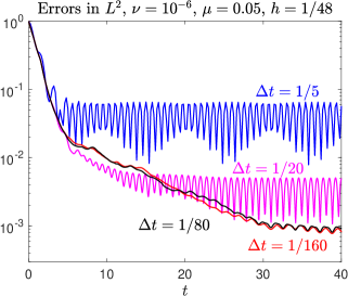
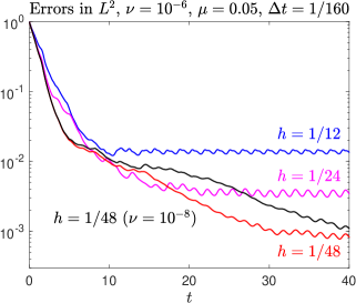
Figure 1: Velocity errors vs $t$ for $\nu=10^{-6}$.

In Fig. 1, it can be seen how the error at the initial time is equal to $1$, decays exponentially with time until reaching the asymptotic regime, where, in this example, its value oscillates periodically. On the left plot, we show the errors for $h=1/48$ and decreasing values of $\Delta t$. In the asymptotic regime, the $O((\Delta t)^{2})$ term dominates the error for the two largest values of $\Delta t$. For the two smallest values of $\Delta t$, the errors are almost identical in the asymptotic regime, meaning that it is the $O(h^{2})$ term that dominates the error. On the right plot in Fig. 1, on the contrary, we show the errors for different values of $h$ but with $\Delta t$ fixed to $\Delta t=1/160$, so that the $O(h^{2})$ term in the error is dominant in the asymptotic regime. Observe that, for $h=1/48$, the asymptotic regime is not reached until $t=35$ approximately. We obtained similar figures (not shown here) for the rest of the values of $\nu$, and in all of them we observed that the asymptotic regime is already reached by $t=35$, except for $\nu=10^{-8}$ and $h=1/48$ (also shown in Fig 1), where it was not reached until $t=42$. For this reason, in the figures that follow, we computed the maximum value of the $L^{2}$ errors in velocity for values of $t_{n}$ in the interval $[35,40]$, except for $\nu=10^{-8}$ and $h=1/48$, which they were on the interval $[42,45]$.

In Fig. 2 we present velocity errors in $L^{2}$ for the four values of $\nu$. For every mesh, the errors obtained with the different values of $\Delta t$ are plotted with crosses for the results corresponding to $\mu=0.05$ and with circular bullets for those corresponding to $\mu=0$, and, for each mesh, the results of the different values of $\Delta t$ are joined by straight segments, with continuous lines for $\mu=0.05$ and discontinuous lines for $\mu=0$.

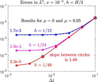
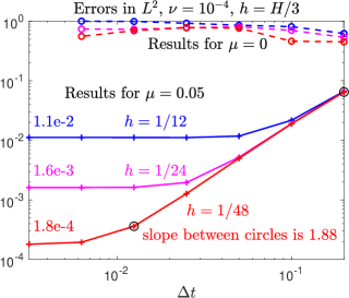
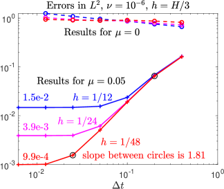
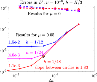
Figure 2: Velocity errors vs $\Delta t$.

To check the order of convergence in time we show the slope of a least squares fit to the results corresponding to $h=1/48$, for the values of $\Delta t$ between the points marked with black circles. It can be seen that all slopes have values between 1.81 and $1.88$, confirming the $O((\Delta t)^{2})$ behaviour of the error whenever the error arising from time integration dominates that arising from spatial discretization. To check the order of convergence in space, we show the error corresponding to $\mu=0.05$ obtained on every mesh with the smallest value of $\Delta t$ used, which, as commented above, we make sure it was sufficiently small so that the spatial error dominates. It can be seen that the error for $\mu=0.05$ behaves as $O(h^{3})$ for $\nu=10^{-2}$ and $10^{-4}$, and $O(h^{2})$ for $\nu=10^{-6}$ or smaller, confirming the second statement in Theorem 3.12 and Remark 3.7. Furthermore, comparing the results for $\nu=10^{-6}$ and $\nu=10^{-8}$, we see that the (spatial) errors are practically the same, confirming that the error constants in the second statement in Theorem 3.12 are independent of $\nu^{-1}$. The only difference that we have found, as shown in Fig. 1, is the slower rate of decay in time of the error in the initial condition for $\nu=10^{-8}$.

With respect to the results corresponding to $\mu=0$, we see a very different behaviour depending on the size of $\nu$. For $\nu=10^{-2}$, they are practically the same as those corresponding to $\mu=0.05$ and, hence, they show an $O(h^{3}+(\Delta t)^{2})$ behaviour, confirming the first statement in Theorem 3.12. For smaller values of $\nu$, however, the negative powers of $\nu$ in the error bounds prevent the method from exhibiting convergence for the values of $h$ and $\Delta t$ shown in Fig. 2 (presumably, convergence will be achieved for much smaller values of $h$). Fig. 2 clearly shows the beneficial effect of the grad-div term when $\nu$ is small.

5 Conclusions

We have obtained error bounds for fully discrete approximations with inf-sup stable mixed finite element methods in space of a continuous downscaling data assimilation method for the two and three-dimensional Navier-Stokes equations. In the data assimilation algorithm measurements on a coarse mesh are given represented by different types of interpolation operators $I_{H}\boldsymbol{u}$, where $I_{H}$ can be an interpolant for non smooth functions or a standard Lagrange interpolant. To our knowledge, only reference [23] and the present paper consider the last case, since in previous references explicit use is made of bounds (24) and (25), which are not valid for nodal (Lagrange) interpolation. In the method, a penalty term is added with the aim of driving the approximation towards the solution $\boldsymbol{u}$ for which the measurements are known. For the time discretization we consider three different methods: the implicit Euler method and an implicit and a semi-implicit second order backward differentiation formula.For the spatial discretization we consider both the Galerkin method and the Galerkin method with grad-div stabilization.

Uniform error bounds in time have been obtained for the approximation to the velocity field $\boldsymbol{u}$ for all the methods, extending the results in [23] where the semi-discretization in space is considered. For the Galerkin method the spatial bounds we prove are optimal, the rate of convergence of the method in $L^{2}$ being $r$ when using piecewise polynomials of degree $r-1$ in the velocity approximation. In the case where grad-div stabilization is added, the constants in the error bounds do not depend on inverse powers of the viscosity parameter $\nu$, which is of importance in many applications where viscosity is orders of magnitude smaller than the velocity. For the Galerkin method with grad-div stabilization a rate of convergence $r-1$ is obtained in the $L^{2}$ norm of the velocity. This bound is sharp, as it is shown in the numerical experiments of the paper. Moreover, it can be clearly observed in the experiments, that for values of the viscosity smaller than $\nu=10^{-4}$ the Galerkin method does not achieve convergence in the range of values of the mesh size for which the Galerkin method with grad-div stabilization converges clearly with the predicted rate of convergence. It is thus to be remarked the dramatic effect of adding grad-div stabilization when the viscosity is small.

In the present paper, as in [23], as opposed to previous references, we do not demand any upper bound on the nudging parameter $\beta$. The authors of [34] had observed (see [34, Remark 3.8]) that the upper bound on $\beta$ they required in the analysis does not hold in the numerical experiments, which is also corroborated by the numerical experiments in [23].

References

[1]
R. A. Adams and J. J. F. Fournier.
Sobolev spaces, volume 140 of Pure and Applied Mathematics
(Amsterdam).
Elsevier/Academic Press, Amsterdam, second edition, 2003.
[2]
S. Agmon.
Lectures on elliptic boundary value problems.
AMS Chelsea Publishing, Providence, RI, 2010.
Prepared for publication by B. Frank Jones, Jr. with the assistance
of George W. Batten, Jr., Revised edition of the 1965 original.
[3]
M. U. Altaf, E. S. Titi, T. Gebrael, O. M. Knio, L. Zhao, M. F. McCabe, and
I. Hoteit.
Downscaling the 2d bénard convection equations using continuous
data assimilation.
Computational Geosciences, 21(3):393–410, June 2017.
[4]
M. Asch, M. Bocquet, and M. Nodet.
Data assimilation, volume 11 of Fundamentals of
Algorithms.
Society for Industrial and Applied Mathematics (SIAM), Philadelphia,
PA, 2016.
Methods, algorithms, and applications.
[5]
B. Ayuso, B. García-Archilla, and J. Novo.
The postprocessed mixed finite-element method for the
Navier-Stokes equations.
SIAM J. Numer. Anal., 43(3):1091–1111, 2005.
[6]
A. Azouani, E. Olson, and E. S. Titi.
Continuous data assimilation using general interpolant observables.
J. Nonlinear Sci., 24(2):277–304, 2014.
[7]
C. Bernardi and V. Girault.
A local regularization operator for triangular and quadrilateral
finite elements.
SIAM J. Numer. Anal., 35(5):1893–1916, 1998.
[8]
F. Brezzi and R. S. Falk.
Stability of higher-order Hood-Taylor methods.
SIAM J. Numer. Anal., 28(3):581–590, 1991.
[9]
F. Brezzi and M. Fortin.
Mixed and hybrid finite element methods, volume 15 of Springer Series in Computational Mathematics.
Springer-Verlag, New York, 1991.
[10]
H. Chen.
Pointwise error estimates for finite element solutions of the
Stokes problem.
SIAM J. Numer. Anal., 44(1):1–28, 2006.
[11]
P. Constantin and C. Foias.
Navier-Stokes equations.
Chicago Lectures in Mathematics. University of Chicago Press,
Chicago, IL, 1988.
[12]
R. Daley.
Navier-Stokes equations.
Cambridge Atmospheric and Space Science Series. Cambridge University
Press, Cambridge, 1991.
[13]
J. de Frutos, B. García-Archilla, V. John, and J. Novo.
Grad-div stabilization for the evolutionary Oseen problem with
inf-sup stable finite elements.
J. Sci. Comput., 66(3):991–1024, 2016.
[14]
J. de Frutos, B. García-Archilla, V. John, and J. Novo.
Analysis of the grad-div stabilization for the time-dependent
Navier-Stokes equations with inf-sup stable finite elements.
Adv. Comput. Math., 44(1):195–225, 2018.
[15]
J. de Frutos, B. García-Archilla, and J. Novo.
Error analysis of projection methods for non inf-sup stable mixed
finite elements: the Navier-Stokes equations.
J. Sci. Comput., 74(1):426–455, 2018.
[16]
A. Farhat, H. Johnston, M. Jolly, and E. S. Titi.
Assimilation of nearly turbulent rayleigh–bénard flow through
vorticity or local circulation measurements: A computational study.
Journal of Scientific Computing, Mar 2018.
[17]
A. Farhat, M. S. Jolly, and E. S. Titi.
Continuous data assimilation for the 2D Bénard convection
through velocity measurements alone.
Phys. D, 303:59–66, 2015.
[18]
A. Farhat, E. S. Lunasin, and E. S. Titi.
On the charney conjecture of data assimilation employing temperature
measurements alone: the paradigm of 3d planetary geostrophic model,.
Math. Clim. Weather Forecast., 2:59–66, 2016.
[19]
L. P. Franca and T. J. R. Hughes.
Two classes of mixed finite element methods.
Comput. Methods Appl. Mech. Engrg., 69(1):89–129, 1988.
[20]
G. P. Galdi.
An introduction to the mathematical theory of the
Navier-Stokes equations. Vol. I, volume 38 of Springer Tracts
in Natural Philosophy.
Springer-Verlag, New York, 1994.
Linearized steady problems.
[21]
B. García-Archilla, J. Novo, and E. S. Titi.
Postprocessing the Galerkin method: a novel approach to approximate
inertial manifolds.
SIAM J. Numer. Anal., 35(3):941–972, 1998.
[22]
B. García-Archilla, J. Novo, and E. S. Titi.
An approximate inertial manifolds approach to postprocessing the
Galerkin method for the Navier-Stokes equations.
Math. Comp., 68(227):893–911, 1999.
[23]
B. García-Archilla, J. Novo, and E. S. Titi.
Uniform in time error estimates for a finite element method applied
to a downscaling data assimilation algorithm for the Navier-Stokes
equations.
arXiv e-prints, page arXiv:1807.08735, Mar. 2018.
[24]
M. Gesho, E. Olson, and E. S. Titi.
A computational study of a data assimilation algorithm for the
two-dimensional Navier-Stokes equations.
Commun. Comput. Phys., 19(4):1094–1110, 2016.
[25]
V. Girault and J.-L. Lions.
Two-grid finite-element schemes for the transient Navier-Stokes
problem.
M2AN Math. Model. Numer. Anal., 35(5):945–980, 2001.
[26]
E. Hairer and G. Wanner.
Solving ordinary differential equations. II, volume 14 of
Springer Series in Computational Mathematics.
Springer-Verlag, Berlin, 2010.
Stiff and differential-algebraic problems, Second revised edition,
paperback.
[27]
K. Hayden, E. Olson, and E. S. Titi.
Discrete data assimilation in the Lorenz and 2D Navier-Stokes
equations.
Phys. D, 240(18):1416–1425, 2011.
[28]
J. G. Heywood and R. Rannacher.
Finite element approximation of the nonstationary Navier-Stokes
problem. I. Regularity of solutions and second-order error estimates for
spatial discretization.
SIAM J. Numer. Anal., 19(2):275–311, 1982.
[29]
J. G. Heywood and R. Rannacher.
Finite element approximation of the nonstationary Navier-Stokes
problem. III. Smoothing property and higher order error estimates for
spatial discretization.
SIAM J. Numer. Anal., 25(3):489–512, 1988.
[30]
H. A. Ibdah, C. F. Mondaini, and E. S. Titi.
Uniform in time error estimates for fully discrete numerical schemes
of a data assimilation algorithm.
arXiv:1805.01595v1, 2018.
[31]
V. John.
Finite element methods for incompressible flow problems,
volume 51 of Springer Series in Computational Mathematics.
Springer, Cham, 2016.
[32]
V. John and A. Kindl.
Numerical studies of finite element variational multiscale methods
for turbulent flow simulations.
Comput. Methods Appl. Mech. Engrg., 199(13-16):841–852, 2010.
[33]
E. Kalnay.
Atmospheric Modeling, Data Assimilation and Predictability.
Cambridge University Press, 2002.
[34]
A. Larios, L. G. Rebholz, and C. Zerfas.
Global in time stability and accuracy of IMEX-FEM data
assimilation schemes for Navier–Stokes equations.
Comput. Methods Appl. Mech. Engrg., 345:1077–1093, 2019.
[35]
K. Law, A. Stuart, and K. Zygalakis.
Data assimilation, volume 62 of Texts in Applied
Mathematics.
Springer, Cham, 2015.
A mathematical introduction.
[36]
E. Lunasin and E. S. Titi.
Finite determining parameters feedback control for distributed
nonlinear dissipative systems—a computational study.
Evol. Equ. Control Theory, 6(4):535–557, 2017.
[37]
C. F. Mondaini and E. S. Titi.
Uniform-in-time error estimates for the postprocessing Galerkin
method applied to a data assimilation algorithm.
SIAM J. Numer. Anal., 56(1):78–110, 2018.
[38]
L. G. Rebholz and C. Zerfas.
Simple and efficient continuous data assimilation of evolution
equations via algebraic nudging.
arXiv e-prints, page arXiv:1810.03512, Oct. 2018.
[39]
S. Reich and C. Cotter.
Probabilistic forecasting and Bayesian data assimilation.
Cambridge University Press, New York, 2015.
[40]
L. Röhe and G. Lube.
Analysis of a variational multiscale method for large-eddy simulation
and its application to homogeneous isotropic turbulence.
Comput. Methods Appl. Mech. Engrg., 199(37-40):2331–2342,
2010.
[41]
A. H. Schatz.
Pointwise error estimates and asymptotic error expansion inequalities
for the finite element method on irregular grids. I. Global estimates.
Math. Comp., 67(223):877–899, 1998.
[42]
A. H. Schatz and L. B. Wahlbin.
On the quasi-optimality in of the -projection into finite element spaces.
Math. Comp., 38(157):1–22, 1982.
[43]
L. R. Scott and S. Zhang.
Finite element interpolation of nonsmooth functions satisfying
boundary conditions.
Math. Comp., 54(190):483–493, 1990.
[44]
C. Taylor and P. Hood.
A numerical solution of the Navier-Stokes equations using the
finite element technique.
Internat. J. Comput. & Fluids, 1(1):73–100, 1973.
[45]
R. Temam.
Navier-Stokes equations, volume 2 of Studies in
Mathematics and its Applications.
North-Holland Publishing Co., Amsterdam, third edition, 1984.
Theory and numerical analysis, With an appendix by F. Thomasset.