Predicting Spatio-Temporal Time Series Using Dimension Reduced Local States

Abstract

We present a method for both cross estimation and iterated time series prediction of spatio temporal dynamics based on reconstructed local states, PCA dimension reduction, and local modelling using nearest neighbour methods. The effectiveness of this approach is shown for (noisy) data from a (cubic) Barkley model, the Bueno-Orovio-Cherry-Fenton model, and the Kuramoto-Sivashinsky model.

1 Introduction

In many experiments some variables of the system are more easily observable than others. If the underlying dynamics is deterministic, in general the observable of interest is nonlinearly related to other variables of the system which might be more accessible. In such cases one may try to estimate any observable which is difficult to measure from time series of those variables which are at one’s disposal. Another task frequently encountered with observed time series is forecasting the dynamical evolution of the system and the time series. To cope with both tasks in case of multivariate time series from extended spatio-temporal systems we present an approach for cross estimation and iterated time series prediction using local state reconstructions, dimension reduction, and nearest neighbour methods for local modelling. Local state reconstruction is motivated by the fact that it often is impractical to predict the behaviour of systems with a large spatial extent all at once. If instead one combines a spatial and temporal neighbourhood around each measurement to find a description of the local system state it becomes possible to make predictions for each point in space independently. For performing cross estimation or prediction based on local states one can either use nearest neighbours methods (also called local modelling) [20] or employ some other black-box modelling approach like, for example, Echo State Machines [21, 27]. In the following, we shall use local modelling by selecting for each reconstructed reference state similar states from a training data set whose relations to other observables and/or future temporal evolutions are known and can be exploited for cross estimation or time-series prediction.

Successful reconstruction of high-dimensional dynamics in extended systems, however, requires very large embedding dimensions which is a major challenge in particular for nearest neighbour methods. Therefore, a crucial point in making the conceptually simple nearest neighbours algorithm performant is dimension reduction. As a means of dimension reduction to find lower a dimensional representation of the local states, we employ principal component analysis (PCA) which turns out to improve performance in particular for noisy data.

2 Predicting Spatio-Temporal Time Series

In this section we shall introduce the main concepts for predicting spatio-temporal time series, including local delay coordinates states, linear dimension reduction, and nearest neighbours methods for local modelling of the dynamical evolution or any other relation between observed time series.

2.1 Local Modelling

Let $\mathbf{x}_{t}$ be a state of some dynamical system evolving in time $t$ and let $s_{t}=h(\mathbf{x}_{t})$ be a signal which can be observed or measured. Furthermore, let’s assume that the dynamical equations generating the flow in state space and the measurement function $h$ are unknown, but only a set ${\cal{S}}$ of $M$ states $\mathbf{x}_{t_{m}}$ and corresponding time series values $s_{t_{m}}$ for $t_{1},\ldots,t_{M}$ are available, for which also future values $\mathbf{x}_{t_{m}+T}$ and $s_{t_{m}+T}$ are known (due to previous measurements, for example). This data set ${\cal{S}}$ can be used to predict the future value $\mathbf{x}_{t+T}$ of a given state $\mathbf{x}_{t}$ or to estimate the corresponding time series values $s_{t}$ and $s_{t+T}$, by selecting the $k$ nearest neighbours of $\mathbf{x}_{t}$ in ${\cal{S}}$ and using their future values (or the corresponding time series values) for approximating $\mathbf{x}_{t+T}$ (or $s_{t}$ and $s_{t+T}$), for example, by (distance weighted) averaging.

In most practical applications of this kind of local nearest neighbour modelling the required states are reconstructed from a measured time series using the concept of delay coordinates (to be introduced in the next section). Local modelling in (reconstructed) state space is a powerful tool for purely data driven time series prediction [3, 13]. Its main ingredients are a proper state space representation of the measured time series, fast nearest neighbour searches, and local models such as low order polynomials which can accurately interpolate and predict the (nonlinear) relation between (reconstructed) states and target values.

2.2 Delay Coordinates

The most important part of time series based local modelling is the representation of data, i.e. proper reconstruction of states from data. Typically this representation is found utilizing delay coordinates and Taken’s Embedding Theorem [25, 22, 15, 2, 8] such that a scalar time series $\{s_{t}\}$ is reconstructed to state vectors

$$\mathbf{x}_{t}=(s_{t-\gamma\tau},\dots,s_{t-\tau},s_{t})$$

by including $\gamma$ past measurements each separated by $\tau$ time steps. For multivariate time series $\{\mathbf{s}_{t}\}$ one can do the same for each of the components resulting is state vectors

$$\mathbf{x}_{t}=(s_{1,t-\gamma\tau},\dots,s_{1,t},s_{2,t-\gamma\tau},\dots,s_{2,t}).$$

2.3 Spatial Embedding

In principle, delay embedding could also be employed to reconstruct (global) states of high-dimensional spatially extended systems using multivariate time series sampled at many spatial locations. Such global state vectors are (and have to be) very high dimensional (for systems exhibiting extensive chaos). The runtime of nearest neighbour searches, however, and in particularly the memory usage of such reconstructions grows rapidly with the dimension of the reconstructed global states. To avoid this issue it has been proposed [19, 20, 18] to reconstruct (spatially) local states and to predict spatially extended systems point by point instead of the whole global state at once. This approach is motivated by the fact that all spatially extended physical systems posses a finite speed at which information travels. Therefore the future value of any of the variables depends solely on its past and its spatial neighbours. Instead of trying to reconstruct the state of the whole system into one vector, we limit ourselves to reconstructing small neighbourhoods of all points that carry enough information to predict one point one time step into the future. As an additional benefit the infeasibly large embedding dimension that would result from embedding the entire space into a single state is greatly reduced. The idea of local state reconstruction was first applied to spatially one-dimensional systems [19, 20, 18] and was used, for example, to anticipate extreme events in extended excitable systems [7].

In the following we will present the embedding procedure for spatiotemporal time series represented by $u_{t,\alpha}$, where $t$ denotes time and $\alpha$ a point in space. For 2D space $\alpha$ takes the values $\alpha=(i,j)\quad\forall 1\leq i\leq N_{x},\,1\leq j\leq N_{y}$.

In the most general case such an embedding could consist of arbitrary combinations of neighbours in all directions of space and time. For practical purposes we will limit ourselves to a certain set of parameters to describe which neighbours will be included into a reconstruction. We parameterize an embedding with the number $\gamma$ of past time steps and their respective temporal delay (or time lag) $\tau$. All neighbours in space that are within the radius $r$, referring to the Euclidean distances in a unit grid, will be included as well. The resulting shape of the embedding is comparable to a cylinder in 2+1D space-time. To make this clearer, a visualization of the spatial embedding in a two-dimensional system is displayed in Fig. 1 for different radii $r$.

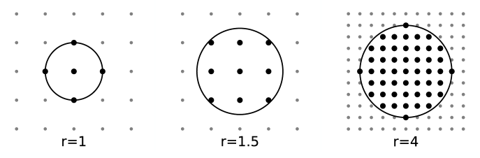
Figure 1: Visualization of spatial embedding for radii $r\in\{1,\,1.5,\,4\}$. All points within the circle spanned by $r$ are included in the embedding.

In the following we shall assume that the dynamics underlying the observed spatio-temporal time series is invariant with respect to translations, i.e. that the system is homogeneous. In this case states reconstructed at different locations can be combined to a single training set providing the data base for cross estimation or time series prediction as will be discussed in more detail in Section 2.4. However, even if the dynamical rules are the same for all locations, special care needs to be taken at the boundaries. This becomes obvious when trying to include nonexistent neighbours from outside the grid. For periodic boundary condition the canonical solution is to wrap around at the edges but for constant boundaries the solution is not so obvious. In many cases the dynamics near the boundary may also differ from dynamics far from it. It is therefore desirable to treat boundaries separately during nearest neighbour predictions. A solution proposed in Ref. [20] is to fill the missing values at the boundary with an additional parameter being a large constant number. If the parameter is significantly larger than typical values of the internal dynamics, the states reconstructed from the boundary fill regions in state space isolated from state vectors of internal dynamics. This has the desired effect as nearest neighbour searches will always find boundary states when given a boundary state as query and similarly for internal states.

2.4 Dimension Reduction

The feasibility of any nearest neighbour search depends heavily on the memory consumption as the whole data set needs to lie in memory. A crucial part of our algorithm is therefore about creating a proper low dimensional reconstruction. In most numerical experiments choosing just very few neighbours to include in the reconstruction did not prove to be very effective. Therefore, instead of choosing a small embedding dimension from the start, we propose to perform some means of dimension reduction on the resulting reconstructed state vectors. For this task we choose Principal Component Analysis (PCA) as it is a straight-forward standard technique for (linear) dimension reduction, where the reconstructed states $\mathbf{x}_{t}$ are projected onto the eigenvectors of the covariance matrix corresponding the largest eigenvalues [14]. In the field of nonlinear time series analysis PCA has first been used by D. Broomhead and G. King [9] who suggested to use dimension reduction applied to high dimensional delay reconstructions with time series densely sampled in time.

Let $\{\mathbf{x}^{n}\}$ be the set of all $N$ reconstructed states $\mathbf{x}^{n}=(x_{1}^{n},\ldots,x_{D_{E}}^{n})\in\mathbb{R}^{D_{E}}$ (at different times $t$ and locations $\alpha$, assuming stationary and spatially homogeneous dynamical rules). To perform PCA first mean values $\mathbf{\bar{x}}=\frac{1}{N}\sum_{n=1}^{N}\mathbf{x}_{n}=(\bar{x}_{1},\ldots,\bar{x}_{D_{E}})$ with $\bar{x}_{i}=\frac{1}{N}\sum_{n=1}^{N}x_{i}^{n}$ are subtracted resulting in shifted states $\mathbf{\tilde{x}}^{n}=\mathbf{x}^{n}-\mathbf{\bar{x}}=(\tilde{x}_{1}^{n},\ldots,\tilde{x}_{D_{E}}^{n})$. The covariance matrix

$$C_{X} = \frac{1}{N}\sum_{n=1}^{N}(\mathbf{\tilde{x}}^{n})^{tr}\cdot\mathbf{\tilde{x}}^{n}$$

$$= \frac{1}{N}\begin{bmatrix}\sum_{n=1}^{N}\tilde{x}_{1}^{n}\tilde{x}_{1}^{n}&\sum_{n=1}^{N}\tilde{x}_{1}^{n}\tilde{x}_{2}^{n}&\ldots&\sum_{n=1}^{N}\tilde{x}_{1}^{n}\tilde{x}_{D_{E}}^{n}\\ \sum_{n=1}^{N}\tilde{x}_{2}^{n}\tilde{x}_{1}^{n}&\sum_{n=1}^{N}\tilde{x}_{2}^{n}\tilde{x}_{2}^{n}&\dots&\sum_{n=1}^{N}\tilde{x}_{2}^{n}\tilde{x}_{D_{E}}^{n}\\ \vdots&\vdots&\ddots&\vdots\\ \sum_{n=1}^{N}\tilde{x}_{D_{E}}^{n}\tilde{x}_{1}^{n}&\sum_{n=1}^{N}\tilde{x}_{D_{E}}^{n}\tilde{x}_{2}^{n}&\ldots&\sum_{n=1}^{N}\tilde{x}_{D_{E}}^{n}\tilde{x}_{D_{E}}^{n}\\ \end{bmatrix}$$

is approximated by iteratively reconstructing individual shifted delay vectors $\mathbf{\tilde{x}}^{n}$ from the dataset and summing the terms $(\mathbf{\tilde{x}}^{n})^{tr}\cdot\mathbf{\tilde{x}}^{n}$ into the preallocated matrix $C_{X}$.

Local states $\mathbf{y}^{n}$ of lower dimension $D_{R}\leq D_{E}$ are obtained by projecting the shifted states $\mathbf{\tilde{x}}$

$$\mathbf{y}^{n}=P\mathbf{\tilde{x}}^{n}$$

using a (globally valid) $D_{R}\times D_{E}$ projection matrix $P$ whose rows are given by the $D_{R}$ eigenvectors of the matrix $C_{X}$ corresponding to the largest $D_{R}$ eigenvalues. The dimensionality $D_{R}$ of the subspace spanned by eigenvectors to be taken into account can either be set explicitly or determined such that some percentage of the original variance of the embedding is preserved.

The whole data set can thus be embedded into the space with reduced dimension $D_{R}$ by embedding each point of the data set into the high dimensional space $\mathbb{R}^{D_{E}}$ and projecting it into the low dimensional space $\mathbb{R}^{D_{R}}$ using the PCA projection matrix $P$ computed beforehand.

For the subsequent prediction process the projected reconstruction vectors $\mathbf{y}^{n}$ are then fed into a tree structure such as a kd-tree [5, 11] for fast nearest neighbour searching.

One issue arises with states near boundaries. Since the dynamics close to the boundaries may differ from the rest of the system, they were separated from other reconstructed vectors in phase space. This was achieved by setting the non-existent neighbours of boundary points to a large constant value [20]. The power of PCA however relies on its assumption of a single cloud of points in (state) space close to a low dimensional linear subspace. This is no longer the case when constant boundaries come into play. To sidestep this issue we suggest changing the second step of the procedure described above. Simply exclude all boundary states from the computation of the projection matrix $P$ but project them with the resulting matrix $P$ nonetheless. In principle this could eliminate the offset meant to separate internal and boundary dynamics but in practice the projection matrices rarely posses zero-valued entries. Therefore it is highly unlikely that this would become a problem as long as boundary offset values are chosen large enough.

2.5 Prediction Algorithm

While the values and the dimension of the state vectors have changed in the dimension reduction process, their ordering $(t,\alpha)\leftrightarrow n$ within the reconstructed space and the search tree is known. It is therefore sufficient to find the indices of nearest neighbours in the dimension reduced reconstructed training set in $\mathbb{R}^{D_{R}}$. To make predictions we assign each reconstructed state $\mathbf{x}_{t,\alpha}$ a target value $\mathbf{z}_{t,\alpha}$ from the original training data and the only difference between temporal prediction and cross estimation lies in the choice of these target values.

For time series prediction we choose $\mathbf{x}_{t,\alpha}\rightarrow u_{t+1,\alpha}$ where $\mathbf{x}_{t,\alpha}$ are the reconstructed vectors from the spatio-temporal time series $\{u_{t,\alpha}\}$ and $u_{t+1,\alpha}$ the target values. The prediction process then consists of reconstructing $\mathbf{x}_{T,\alpha}$ from the end of the time series by applying the same embedding parameters, subsequent dimension reduction using the projection matrix $P$ that was computed for the training set, and local nearest neighbour modelling providing the target values $u_{T+1,\alpha}$. Once a prediction for each point (denoted by $\alpha$) has been made, all future values $u_{T+1,\alpha}$ of the (input) field $u$ are known and the procedure can be repeated for predicting $u_{T+2,\alpha}$. Using this kind of iterated prediction spatio-temporal time series can, in principle, be forecasted for any period of time (with the well-known limits of predictability of chaotic dynamics).

The case of cross estimation is even simpler than time series prediction. Here we are given a training set of two fields: an input variable $u_{t,\alpha}$ and a target variable $v_{t,\alpha}$. The values of the input field $u_{t,\alpha}$ are reconstructed into delay vectors $\mathbf{x}_{t,\alpha}$. Using PCA and nearest neighbours search we find similar reconstructed states in the training set for which the corresponding values of the target variables are known and can be used for estimating the current target $v_{t,\alpha}$.

2.6 Error Measures

In the next section we will test the presented prediction methods on the model systems described in section 3. For evaluation we compare any predicted field $\hat{v}$ with the corresponding correct values (i.e. test values) $\check{v}$ by considering spatial averages over all sites $\alpha$. This so-called Mean Squared Error (MSE) is then normalized by the MSE obtained when using the (spatial) mean value $\bar{v}$ for prediction. The resulting Normalized Mean Squared Error (NRMSE) is defined as

$$\text{\text{NRMSE}}(\check{v},\hat{v})=\sqrt{\frac{\text{\text{MSE}}(\check{v},\hat{v})}{\text{\text{MSE}}(\check{v},\bar{v})}},\hskip 14.22636pt\text{where}\hskip 14.22636pt\text{\text{MSE}}(\check{v},\hat{v})=\frac{1}{A}\sum_{\alpha}\left(\check{v}_{\alpha}-\hat{v}_{\alpha}\right)^{2}$$ (1)

where $A$ is the number of spatial sites $\alpha$ taken into account. Any good estimate or forecast should be (much) better than the trivial prediction using mean values and result in NMSE values (much) smaller than one.

2.7 Software

All software used in this paper has been published in the form of an open source software library under the name of TimeseriesPrediction.jl [1] along with extensive documentation and various examples. It is written using the programming language Julia [6] with extensibility in mind, such that it is compatible with different spatial dimensions as well as arbitrary spatiotemporal embeddings. This is made possible through a modular design and Julia’s multiple dispatch.

3 Model Systems

The Kuramoto-Sivashinsky (KS) model [17, 23, 24] has been devised for modelling flame fronts and will in our case be used as a benchmark system for iterated time series prediction. The Barkley model [4] describes an excitable medium that shows chaotic interplay of traveling waves. The third and most complex model is the Bueno-Orovio-Cherry-Fenton (BOCF) model [10], which is composed of four coupled fields describing electrical excitation waves in the heart muscle.

3.1 Kuramoto-Sivashinsky System

The Kuramoto-Sivashinsky (KS) system [17, 23, 24] is defined by the following partial differential equation:

$$\frac{\partial u}{\partial t}+\frac{\partial^{2}u}{\partial x^{2}}+\frac{\partial^{4}u}{\partial x^{4}}+\left|\frac{\partial u}{\partial x}\right|^{2}=0$$ (2)

typically integrated with periodic boundary conditions. It is widely used in literature [20, 21] because it is a simple system consisting of just one field while still showing highdimensional chaotic dynamics.

The dynamics were simulated with an EDTRK4 algorithm [12, 16] and the parameters for integration are the time step $\Delta t=0.25$ and the system size $L$ with spatial sampling $Q$. Two example evolutions with $L=22$, $Q=64$ and $L=200$, $Q=512$ are shown in Fig. 2.

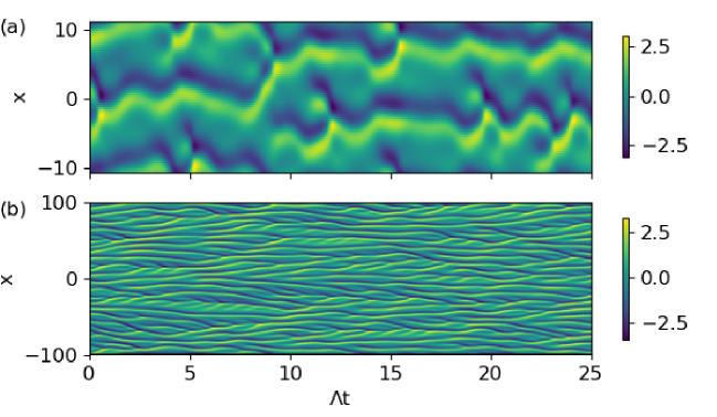
Figure 2: Temporal evolution of the KS model (2) for two different system sizes. Pane (a) has parameters $L=22$ and $Q=64$, while the larger system (b) has $L=200$ and $Q=512$.

3.2 Barkley Model

The Barkley model [4] is a simple system that exhibits excitable dynamics. We will use a modification with a cubic $u^{3}$ term that can be used to generate spatio-temporal chaos such that:

$$\begin{aligned} \frac{\partial u}{\partial t}=&\,\frac{1}{\varepsilon}u(1-u)\left(u-\frac{v+b}{a}\right)+D\nabla^{2}u\\ \frac{\partial u}{\partial t}=&\,u^{3}-v,\end{aligned}$$ (3)

where the parameter set $a=0.75$, $b=0.06$, $\varepsilon=0.08$ and $D=0.02$ leads to chaotic behavior. For integration we used $\Delta t=0.01$ and $\Delta x=0.1$ in combination with an optimized FTCS scheme like the one described in [4].

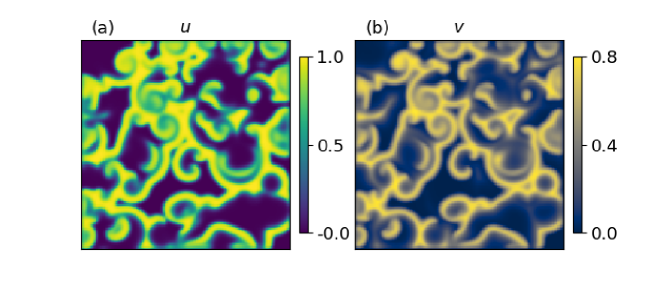
Figure 3: Snapshot of the chaotic Barkley model (3) on a grid of size $150\times 150$ with constant boundary conditions and after transients decayed. The $u$ variable is displayed in (a) and $v$ in (b).

3.3 Bueno-Orovio-Cherry-Fenton Model

The Buono-Orovio-Cherry-Fenton (BOCF) model [10] is a more advanced set of equations that serves as a realistic but relatively simple model of (chaotic) cardiac dynamics. It consist of four coupled fields that can be integrated as PDEs on various geometries. For the sake of simplicity we consider a two-dimensional square. The four variables $u$, $v$, $w$, $s$ are given by the following equations:

$$\begin{aligned} \frac{\partial u}{\partial t}=&D\cdot\nabla^{2}u-(J_{si}+J_{fi}+J_{so})\\ \frac{\partial v}{\partial t}=&\frac{1}{\tau_{v}^{-}}(1-H(u-\theta_{v}))(v_{\infty}-v)-\frac{1}{\tau_{v}^{+}}H(u-\theta_{v})v\\ \frac{\partial w}{\partial t}=&\frac{1}{\tau_{w}^{-}}(1-H(u-\theta_{w}))(w_{\infty}-w)-\frac{1}{\tau_{w}^{+}}H(u-\theta_{w})w\\ \frac{\partial s}{\partial t}=&\frac{1}{2\tau_{s}}((1+\tanh(k_{s}(u-u_{s})))-2s)\end{aligned}$$ (4)

where the currents $J_{si}$, $J_{fi}$ and $J_{so}$ and all other parameters are defined in the appendix. Variable $u$ represents the voltage across the cell membrane and provides spatial coupling due the diffusion term, whereas $v$, $w$, and $s$ are governed by local ODEs without any spatial coupling. Fig. 4 shows a snapshot of all four fields. To make it easier to tell the different fields apart each one has been assigned its own color map that will be used consistently. For simulation we used an implementation by Roland Zimmermann [27], that simulates the dynamics of the BOCF model using an FTCS scheme on a $500\times 500$ grid with integration parameters $\Delta x=1$, $\Delta t=0.1$, diffusion constant $D=0.2$, no-flux boundary conditions and a temporal sampling of $t_{\text{sample}}=2.0$. The dense spatial sampling is needed for integration but impractical for our use. Therefore the software by Zimmermann coarse-grains the data to a grid of size $150\times 150$.

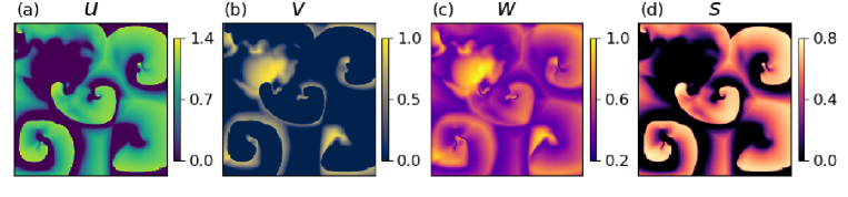
Figure 4: Snapshot of the BOCF model simulated on a $500\times 500$ grid and coarse grained to a $150\times 150$ grid using the software by Zimmermann [27].

4 Cross Estimation

For cross estimation we analyze the Barkley model and the BOCF model. In the beginning both systems are simulated for more than $10000$ time steps so that different subsets can be chosen for model training and testing. All training sets consisted of 5000 consecutive time steps. Due to the dense temporal sampling the first few frames after the end of the training set are potentially predicted much better than the following ones, because data points nearly identical to the desired estimation output are already included in the training set. To avoid this predictions were offset by 1000 frames after the end of the training sequence and averaged over 20 predicted frames to reduce fluctuations and compute a standard deviation for the error measures.

To simulate uncertainty in measurements normally distributed random numbers were added to the observed variable in the test set. Adding such noise with mean $\mu=0$ and standard deviation $\sigma_{\mathcal{N}}=0.075$ resulted in signal-to-noise ratios

$$\text{SNR}_{\text{db}}=10\log_{10}\frac{\left<u_{t,\alpha}^{2}\right>}{\sigma_{\mathcal{N}}^{2}}$$

of 18.5dB and 14.6dB for $u$ and $v$ in the Barkley model, respectively. For the fields $u,v,w,s$ of the BOCF model SNRs were 20.1dB, 13.2dB, 18.1dB, and 15.4dB, respectively. For an intuition of the noisyness Fig. 5 shows the variable $u$ and $v$ of the Barkley model and the variables $u$ and $w$ of the BOCF model with added noise.

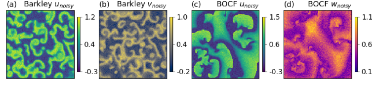
Figure 5: Snapshots of the variables $u$ and $v$ of the Barkley model and the variable $u$ and $w$ of the BOCF model after addition of normally distributed noise.

4.1 Barkley Model

For the Barkley model (3) only the $u$ variable has a diffusion term. Therefore the dynamics of $v$ solely depends on $u$ and its past. This significantly reduces the reconstruction parameter space as spatial neighbourhoods may only be needed for noise reduction during PCA and can likely be small. For the prediction direction $u\rightarrow v$ the best embedding found by optimization, the one with least prediction error, was $\gamma=500$, $\tau=1$ and $r=0$. These parameters produce a highly redundant embedding which allows PCA to efficiently filter out noise. The other direction $v\rightarrow u$ needs spatial neighbourhoods for effective cross prediction and the embedding parameters were $\gamma=30$, $\tau=5$ and $r=3$.

The results evaluated according to the error measure (1) are listed in Table 1. A visualization of the predictions is shown in Fig. 6 along with additional predictions performed with identical parameters but for noiseless input.

	$u\rightarrow v$	$v\rightarrow u$
$\gamma$	500	30
$\tau$	1	5
$r$	0	3
$D_{E}$	501	899
$D_{R}$	15	15
NRMSE	$0.0354\pm 0.0013$	$0.096\pm 0.006$

Table 1: Optimal embedding parameters and cross estimation errors for noisy data from the Barkley model (3) with temporal sampling $t_{\text{sample}}=0.01$. $D_{E}$ is the initial embedding dimension (a direct result of the reconstruction parameters chosen) and $D_{R}$ is the reduced dimension used to make the prediction. For both predictions we used the constant value of 200 for the beyond the boundary pixels. The errors are averaged over 20 predicted frames.

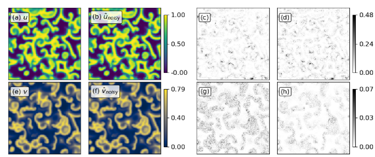
Figure 6: Cross estimation of data generated by the Barkley model (3) from a noisy $v$ field to $u$ and vice versa. (a)-(d) show estimates of the $u$ field where (a) is the actual $u$ field, (b) the predicted field $\hat{u}$ (from noisy input), (c) the absolute difference between the two, and (d) a reference estimation error for noiseless input with identical embedding parameters and training set. Panes (e)-(h) show the same for the field $v$. The embedding parameters are listed in Table 1.

4.2 BOCF Model

Similarly to the Barkley model only the $u$ variable of the BOCF model (4) has a diffusion term which simplifies the predictions of $u\rightarrow\{v,w,s\}$. All embedding parameters, found with a stochastic gradient decent procedure, are listed along with the prediction errors in Table 2. In most of these cases we observe a very large temporal embedding with a small spatial neighbourhood. This is likely due to the dense temporal sampling relative to the propagation speed of wavefronts within the simulated medium. In this way the highly redundant embedding and PCA for dimension reduction provide an effective method of noise reduction. The $w$ field however presents itself as a somewhat smeared out version of the other variables thus requiring a larger spatial neighbourhood to recover the positions of wavefronts.

To visualize a few results we chose the best and worst performing estimations. Figure 7 contains results for $w_{noisy}\rightarrow\{u,v,s\}$ and Fig. 8 shows estimations from a noisy $u$ field to all other variables. The NRMSE values in Table 2 indicate that the estimations from field $w$ perform about one order of magnitude worse than the estimations from field $u$. Figures 7 and 8 on the other hand reveal that, even in the latter estimations, the erroneous pixels are concentrated around the wavefronts. Thus the overall prediction for most of the area is very accurate in both cases.

	$\gamma$	$\tau$	$r$	$D_{E}$	$D_{R}$	NRMSE
$u\rightarrow v$	100	1	1	505	10	$0.037\pm 0.006$
$u\rightarrow w$	100	1	1	505	15	$0.048\pm 0.007$
$u\rightarrow s$	100	1	1	505	15	$0.034\pm 0.004$
$v\rightarrow u$	50	3	2	663	25	$0.093\pm 0.015$
$v\rightarrow w$	200	1	1	1005	25	$0.053\pm 0.011$
$v\rightarrow s$	200	1	1	1005	25	$0.081\pm 0.015$
$w\rightarrow u$	10	2	4	539	9	$0.25\pm 0.03$
$w\rightarrow v$	10	2	4	539	9	$0.25\pm 0.04$
$w\rightarrow s$	10	2	4	539	9	$0.21\pm 0.03$
$s\rightarrow u$	50	1	1.5	459	20	$0.050\pm 0.005$
$s\rightarrow v$	100	1	1	505	15	$0.060\pm 0.009$
$s\rightarrow w$	100	1	1	505	15	$0.070\pm 0.008$

Table 2: Embedding parameters and cross estimation errors, averaged over 20 frames, for noisy data from the BOCF model (4) with temporal sampling of $t_{\text{sample}}=2.0$. A value of 200 was used for the pixels beyond the boundary. $D_{E}$ is the original reconstruction dimension and $D_{R}$ is the reduced dimension used for nearest neighbour searches.

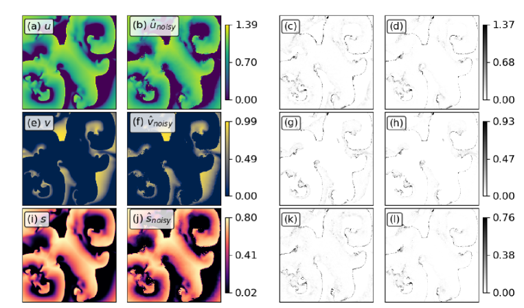
Figure 7: Cross estimation of data generated by the BOCF model (4) from $w_{noisy}$ to all three other variables. (a)-(d) show estimates of the $u$ field where (a) is the actual $u$ field, (b) the predicted field $\hat{u}$ (from noisy input), (c) the absolute difference between the two, and (d) a reference estimation error for noiseless input with identical embedding parameters and training set. Panes (e)-(h) and (i)-(l) show the same for their fields $v$ and $s$, respectively. The embedding parameters are listed in Table 2.

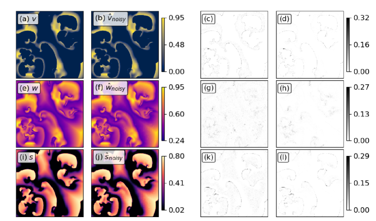
Figure 8: Cross estimation of data generated by the BOCF model (4) from $u_{noisy}$ to all three other variables. (a)-(d) show estimations for the $v$ field where (a) is the actual $v$ field, (b) the predicted field (from noisy input), (c) the absolute difference between the two, and (d) a reference estimation error for noiseless input with identical embedding parameters and training set. Panes (e)-(h) and (i)-(l) show the same for their fields $w$ and $s$, respectively. The embedding parameters are listed in Table 2.

5 Iterated Time Series Prediction

In the following we will analyze the performance of local modelling for spatially extended systems in the context of iterated time series prediction. For this we use the Kuramoto-Sivashinsky model (2) and the Barkley model (3).

The obvious performance measure in this case is the time it takes before the prediction errors exceed a certain threshold. Time however is not an absolute concept in dimensionless systems. Therefore we will also define characteristic timescales of each system which will give a context to the prediction times.

5.1 Predicting Barkley Dynamics

The datasets used during cross estimation were sampled with $t_{\text{sample}}=0.01$ which could be considered nearly continuous relative to the timescale of the dynamics. To provide a useful example for temporal prediction with a reasonable amount of predicted frames we use a larger time step $t_{\text{sample}}=0.2$ (simulation time step was still sufficiently small for accurate numeric integration).

Figure 9 shows one such prediction of the $u$ variable in the Barkley model. The figure consists of seven subplots where the top two rows show the system state at the prediction time steps $n=25,50$ as well as the corresponding iterated predictions. The very right column displays the absolute errors of the prediction defined by $|u_{t,\alpha}-\hat{u}_{t,\alpha}|$. At the bottom is the time evolution of the NRMSE for the prediction. Looking closely at the snapshots in the figure reveals that indeed the maximum prediction error increases quickly, as can be seen by the dark spots of the error plots (c) and (f). The overall error however increases much more slowly which is confirmed by comparing the original state with the prediction.

To set the above results into perspective we calculate a characteristic timescale for the Barkley model. Here we will use the average time between two consecutive local maxima for each pixel, which in good approximation gives the average period of the rotating spiral waves. Averaging over $100\times 100$ pixels and 4000 time steps gave this time as $t_{c}=4.81$. This means that the error of the $u$ field prediction increased to $\text{NRMSE}(u,2t_{c})\approx 0.5$ within two characteristic times.

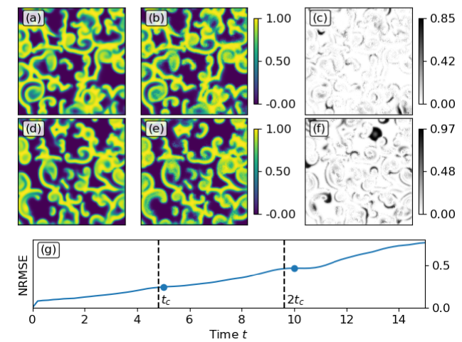
Figure 9: Predicting field $u$ of the Barkley model with system size $150\times 150$ and training of 5000 states. The embedding parameters are $\gamma=12$, $\tau=2$, $r=4$, boundary value $200$. PCA reduced the dimension from $D_{E}=637$ to $D_{R}=15$. Panes (a) and (d) show the true evolution at time $t=5$ and $t=10$. Panes (b) and (e) contain the iterated prediction at that time and (c) and (f) the corresponding absolute error. (g) shows the accumulation of the NRMSE in the prediction. The dashed lines note $t_{c}$, the bullets note the times 5 and 10.

5.2 Predicting Kuramoto-Sivashinsky Dynamics

The Kuramoto-Sivashinsky (KS) model (2) is a one dimensional system that has just a single field. As in the iterated time series prediction of the Barkley model we will need a characteristic timescale for the dynamics of the KS model to assess the quality of the forecast. The approach of measuring wave-front-return-times proved not to be as effective. Instead we will use the Lyapunov time which was defined and calculated for the KS model by Pathak et al. [21]. The following figures are scaled according to the Lyapunov time $\Lambda t$ with $\Lambda\approx 0.1$.

It is possible to integrate the KS model with different sizes $L$ and spatial samplings $Q$. We will attempt to predict the time evolution for $L=22$, $Q=64$ and a larger system with $L=200$ and $Q=512$. The smaller one of the two has just 64 points and thereby could be predicted by reconstructing either local or global states, where the latter are given by combining samples from all $Q$ sites in a state vector. The global states have a higher dimension and need larger training sets to densely fill the reconstructed space but in return each vector represents the state of the whole system. Both approaches are compared in Fig. 10 using the same training set of $9\cdot 10^{5}$ states. For smaller training sets the global state prediction fails altogether as the high dimensional embedding space is too sparsely sampled and nearest neighbour searches always find the same state over and over again. The local state prediction on the other hand still predicts well for some time as is shown in the same figure.

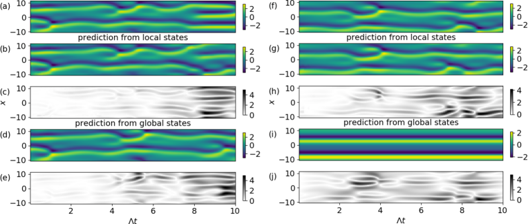
Figure 10: Predictions of the KS dynamics using PCA and 5 nearest neighbours. Shown are: In (a) and (f) actual evolutions, below it in (b) and (g) predictions from local states with parameters $\gamma=7,\,\tau=1,\,r=10$, and at the bottom in (d) and (i) predictions using global states ($\gamma=0,\,r=32$), each along with its errors. The left panel was generated using a training set consisting of $9\cdot 10^{5}$ states and while the right one used $1\cdot 10^{5}$ training states.

A notable observation with the KS model is its variable predictability as it strongly depends on the initial conditions i.e. the current position on the chaotic attractor. Figure 11 shows two predictions using $10^{5}$ training states and identical (reconstruction) parameters. The only difference is that the training set chosen from pre-generated data was offset by 4000 states as compared to the other. The results differ greatly. In one case the errors stay small for roughly 8 Lyapunov times while the other diverges already after 3 Lyapunov times.

Similar variations in predictability were not observed in the KS system with $L=200$ and $Q=512$, which may be due to the significantly larger extent of the system. Instead predictions rarely stayed correct for more than two Lyapunov times. An example is shown in Fig. 12.

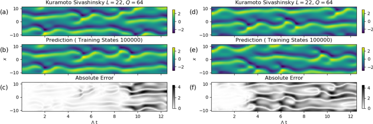
Figure 11: Two predictions of the KS dynamics with $L=22,\,Q=64$. All parameters were identically $\gamma=7,\,\tau=10,\,r=10$ using $10^{5}$ training states, PCA, and 1 nearest neighbour for local modelling. The only difference lies in the initial condition. (a) and (d) show the true evolution, (b) and (e) the predictions, and (c) and (f) the corresponding absolute errors.

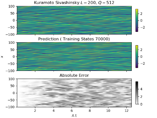
Figure 12: Prediction of the KS dynamics with system parameters $L=200$, $Q=512$ and training of 70000 states. The embedding parameters are $\gamma=2$, $\tau=4$, $r=10$ with PCA and just one nearest neighbour for local modelling.

The issue of variations in predictability of the KS model hinder direct comparisons to the work of Pathak et al. [21] who did not address this problem. In the small system we saw initial conditions where predictions outperformed the ones by Pathak et al. but also others that were much worse. The larger system however has so far been harder to predict and we did not match the prediction accuracy of the approach of Pathak et al.

5.3 Benchmark of PCA

In this paper we use principal component analysis for two reasons. The obvious purpose is to find a low-dimensional representation of the high-dimensional embedding. One very much wanted side-effect is noise reduction. All of the above presented examples used highly redundant embeddings to allow for noise reduction.

To evaluate how well PCA is suited for this purpose we test two things: Does PCA find a low dimensional representation? This is tested in Fig. 13. We see the dependence of the prediction error on the output dimension of PCA in a cross estimation of $u\rightarrow v$ in the Barkley model. It is evident that in this case no more than about $5-7$ dimensions are needed to encode all information relevant to the prediction.

To test whether PCA also successfully eliminated the noise in the test set we compare the two panes in Fig. 13 where the results in the right pane were computed using a 20 times less redundant embedding. The noiseless predictions perform similarly well in both cases, indicating that the additional embedding dimensions are indeed redundant and do not add much information to the reconstructed states. Comparing the noisy predictions highlights the effectiveness of PCA in this case as predictions from the redundant embedding (Fig. 13a) are consistently better by one order of magnitude (comp. Fig 13b).

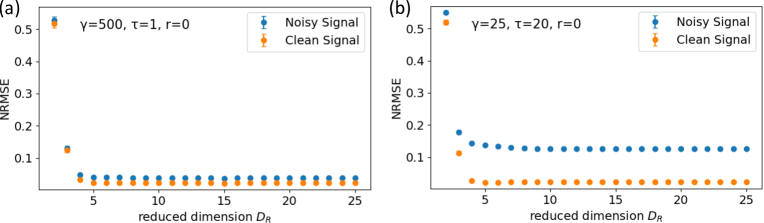
Figure 13: Normalized Mean Squared Errors of cross estimation $u\rightarrow v$ of Barkley variables vs. reduced dimension $D_{R}$ for clean and noisy input signals $u$ with different embedding parameters ((a) $\gamma=500$, $\tau=1$; (b) $\gamma=25$, $\tau=20$) such that $\gamma\tau$ remains constant. The estimation error increases for very small values of the reduced dimension $D_{R}$, but becomes almost constant for $D_{R}>5$. For noisy data PCA based dimension reduction based on higher dimensional embedding with $D_{E}=\gamma+1=501$ in (a) enables a more efficient noise reduction than the reconstruction with $D_{E}=\gamma+1=26$ in (b).

6 Conclusions

The combination of local modelling and principal component analysis for dimension reduction provides a conceptually simple yet effective approach to both cross estimation and temporal prediction of complex spatially extended dynamics. The equations for all three model systems (Barkley model, BOCF model, KS model) were only needed for data generation and as such the approach could well be applied to real world data where the underlying dynamics are not known. Adding noise to the input data naturally reduces prediction quality but in section 5.3 it was shown that PCA can restore accuracy from a more redundant embedding.

7 Acknowlegdements

The authors thank R. Zimmermann for allowing the use of BOCF model simulation and S. Luther for scientific discussions and continuous support.

8 Appendix

8.1 Bueno-Orovio-Cherry-Fenton Model

$H(\cdot)$ denotes the Heaviside function and the currents $J_{fi},\,J_{so},\,J_{si}$ of the Buono-Orovio-Cherry-Fenton (BOCF) model (4) [10] are defined as:

$$J_{fi}= \frac{-v}{\tau_{fi}}H(u-\theta_{v})(u-\theta_{v})(u_{u}-u)$$

$$J_{so}= \frac{1}{\tau_{o}}(u-u_{o})(1-H(u-\theta_{w}))+\frac{1}{\tau_{so}}H(u-\theta_{w})$$

$$J_{si}= \frac{-1}{\tau_{si}}H(u-\theta_{w})ws.$$

The $\tau$ parameters used above are not constant but rather a function of the cell membrane voltage variable $u$:

$$\tau_{v}^{-}= (1-H(u-\theta_{v}^{-}))\tau_{v1}^{-}+H(u-\theta_{v}^{-})\tau_{v2}^{-}$$

$$\tau_{w}^{-}= \tau_{w1}^{-}+\frac{1}{2}(\tau_{w2}^{-}-\tau_{w1}^{-})(1+\tanh(k_{w}^{-}(u-u_{w}^{-})))$$

$$\tau_{so}^{-}= \tau_{so1}+\frac{1}{2}(\tau_{so2}-\tau_{so1})(1+\tanh(k_{so}(u-u_{so})))$$

$$\tau_{s}= (1-H(u-\theta_{w}))\tau_{s1}+H(u-\theta_{w})\tau_{s2}$$

$$\tau_{o}= (1-H(u-\theta_{o}))\tau_{o1}+H(u-\theta_{o})\tau_{o2}$$

and

$$v_{\infty}= \begin{cases}1,u<\theta_{v}^{-}\\ 0,u\geq\theta_{v}^{-}\end{cases}$$

$$w_{\infty}= (1-H(u-\theta_{o}))\left(1-\frac{u}{\tau_{w\infty}}\right)+H(u-\theta_{o})w_{\infty}^{*}.$$

All other parameters are listed in Table 3.

$u_{o}$	0
$u_{u}$	1.58
$\theta_{v}$	0.3
$\theta_{w}$	0.015
$\theta_{v}^{-}$	0.015
$\theta_{o}$	0.006
$\tau_{v1}^{-}$	60

$\tau_{v2}^{-}$	1150
$\tau_{v}^{+}$	1.4506
$\tau_{w1}^{-}$	70
$\tau_{w2}^{-}$	20
$k_{w}^{-}$	65
$u_{w}^{-}$	0.03
$\tau_{w}^{+}$	280

$\tau_{fi}$	0.11
$\tau_{o1}$	6
$\tau_{o2}$	6
$\tau_{so1}$	43
$\tau_{so2}$	0.2
$k_{so}$	2
$u_{so}$	0.65

$\tau_{s1}$	2.7342
$\tau_{s2}$	3
$k_{s}$	2.0994
$u_{s}$	0.9087
$\tau_{si}$	2.8723
$\tau_{w\infty}$	0.07
$w_{\infty}^{*}$	0.94

Table 3: Parameter set for the BOCF model [10] that imitates the Ten Tusscher-Noble-Noble-Panfilov model [26].

References

- [1] Prediction of timeseries using methods of nonlinear dynamics and timeseries analysis: JuliaDynamics/TimeseriesPrediction.jl. URL https://github.com/JuliaDynamics/TimeseriesPrediction.jl
- [2] Abarbanel, H.D.: Analysis of Observed Chaotic Data. Springer-VBerlag, New York (1096). DOI 10.1007/978-1-4612-0763-4
- [3] Atkeson, C.G., Moore, A.W., Schaal, S.: Locally weighted learning. Artificial Intelligence Review 11(1), 11–73 (1997). DOI 10.1023/A:1006559212014. URL https://doi.org/10.1023/A:1006559212014
- [4] Barkley, D.: A model for fast computer simulation of waves in excitable media. Physica D: Nonlinear Phenomena 49(1), 61–70 (1991). DOI 10.1016/0167-2789(91)90194-E. URL http://www.sciencedirect.com/science/article/pii/016727899190194E
- [5] Bentley, J.L.: Multidimensional Binary Search Trees Used for Associative Searching. Commun. ACM 18(9), 509–517 (1975). DOI 10.1145/361002.361007. URL http://doi.acm.org/10.1145/361002.361007
- [6] Bezanson, J., Edelman, A., Karpinski, S., Shah, V.: Julia: A Fresh Approach to Numerical Computing. SIAM Review 59(1), 65–98 (2017). DOI 10.1137/141000671. URL https://epubs.siam.org/doi/10.1137/141000671
- [7] Bialonski, S., Ansmann, G., Kantz, H.: Data-driven prediction and prevention of extreme events in a spatially extended excitable system. Phys. Rev. E 92, 042910 (2015). DOI 10.1103/PhysRevE.92.042910. URL https://link.aps.org/doi/10.1103/PhysRevE.92.042910
- [8] Bradley, E., Kantz, H.: Nonlinear time-series analysis revisited. Chaos: An Interdisciplinary Journal of Nonlinear Science 25(9), 097610 (2015). DOI 10.1063/1.4917289. URL https://doi.org/10.1063/1.4917289
- [9] Broomhead, D., King, G.P.: Extracting qualitative dynamics from experimental data. Physica D: Nonlinear Phenomena 20(2), 217 – 236 (1986). DOI https://doi.org/10.1016/0167-2789(86)90031-X. URL http://www.sciencedirect.com/science/article/pii/016727898690031X
- [10] Bueno-Orovio, A., Cherry, E.M., Fenton, F.H.: Minimal model for human ventricular action potentials in tissue. Journal of Theoretical Biology 253(3), 544–560 (2008). DOI 10.1016/j.jtbi.2008.03.029. URL http://www.sciencedirect.com/science/article/pii/S0022519308001690
- [11] Carlsson, K.: NearestNeighbors.jl: High performance nearest neighbor data structures and algorithms for Julia (2018). URL https://github.com/KristofferC/NearestNeighbors.jl
- [12] Cvitanović, P., Artuso, R., Mainieri, R., Tanner, G., Vattay, G.: Chaos: Classical and Quantum. Niels Bohr Inst., Copenhagen (2016). URL http://ChaosBook.org/. Citation Key: ChaosBook
- [13] Engster, D., Parlitz, U.: Local and Cluster Weighted Modeling for Time Series Prediction. In: B. Schelter, t. Winterhalder, J. Timmer (eds.) Handbook of Time Series Analysis, pp. 39–65. Wiley-VCH Verlag (2006). DOI 10.1002/9783527609970.ch3. URL http://onlinelibrary.wiley.com/doi/10.1002/9783527609970.ch3/summary
- [14] Gareth, J., Witten, D., Hastie, T., Tibshirani, R.: An Introduction to Statistical Learning. Springer, New York (2015). DOI DOI10.1007/978-1-4614-7138-7
- [15] Kantz, H., Schreiber, T.: Nonlinear Time Series Analysis. Cambridge University Press (2004). Google-Books-ID: RfQjAG2pKMUC
- [16] Kassam, A.K., Trefethen, L.N.: Fourth-Order Time-Stepping for Stiff PDEs. SIAM Journal on Scientific Computing 26(4), 1214–1233 (2005). DOI 10.1137/S1064827502410633. URL http://epubs.siam.org/doi/10.1137/S1064827502410633
- [17] Kuramoto, Y.: Diffusion-Induced Chaos in Reaction Systems. Progress of Theoretical Physics Supplement 64, 346–367 (1978). DOI 10.1143/PTPS.64.346. URL https://academic.oup.com/ptps/article/doi/10.1143/PTPS.64.346/1871466
- [18] Mandelj, S., Grabec, I., Govekar, E.: Nonparametric statistical modeling of spatiotemporal dynamics based on recorded data. Int. J. of Bifurcation and Chaos 14(6), 2011–2025 (2004)
- [19] Parlitz, U.: Nonlinear time-series analysis. In: J.A. Suykens, J. Vandewalle (eds.) Nonlinear Modeling - Advanced Black-Box Techniques, pp. 209–239. Springer, Boston, MA (1998). URL https://doi.org/10.1007/978-1-4615-5703-6
- [20] Parlitz, U., Merkwirth, C.: Prediction of Spatiotemporal Time Series Based on Reconstructed Local States. Physical Review Letters 84(9), 1890–1893 (2000). DOI 10.1103/PhysRevLett.84.1890. URL https://link.aps.org/doi/10.1103/PhysRevLett.84.1890
- [21] Pathak, J., Hunt, B., Girvan, M., Lu, Z., Ott, E.: Model-Free Prediction of Large Spatiotemporally Chaotic Systems from Data: A Reservoir Computing Approach. Physical Review Letters 120(2) (2018). DOI 10.1103/PhysRevLett.120.024102. URL https://link.aps.org/doi/10.1103/PhysRevLett.120.024102
- [22] Sauer, T., A. Yorke, J., Casdagli, M.: Embedology. Journal of Statistical Physics 65, 579–616 (1991). DOI 10.1007/BF01053745
- [23] Sivashinsky, G.: On Flame Propagation Under Conditions of Stoichiometry. SIAM Journal on Applied Mathematics 39(1), 67–82 (1980). DOI 10.1137/0139007. URL https://epubs.siam.org/doi/10.1137/0139007
- [24] Sivashinsky, G.I.: Nonlinear analysis of hydrodynamic instability in laminar flames—I. Derivation of basic equations. In: P. Pelcé (ed.) Dynamics of Curved Fronts, pp. 459–488. Academic Press, San Diego (1988). DOI 10.1016/B978-0-08-092523-3.50048-4. URL http://www.sciencedirect.com/science/article/pii/B9780080925233500484
- [25] Takens, F.: Detecting Strange Attractors in Turbulence. Dynamical Systems and Turbulence 898, 366–381 (1981)
- [26] ten Tusscher, K.H.W.J., Noble, D., Noble, P.J., Panfilov, A.V.: A model for human ventricular tissue. American Journal of Physiology-Heart and Circulatory Physiology 286(4), H1573–H1589 (2004). DOI 10.1152/ajpheart.00794.2003. URL https://www.physiology.org/doi/full/10.1152/ajpheart.00794.2003
- [27] Zimmermann, R.S., Parlitz, U.: Observing spatio-temporal dynamics of excitable media using reservoir computing. Chaos: An Interdisciplinary Journal of Nonlinear Science 28(4), 043118 (2018). DOI 10.1063/1.5022276. URL https://aip.scitation.org/doi/10.1063/1.5022276