Real-time reconstruction of moving point/dipole wave sources from boundary measurements

Abstract

This paper is concerned with a reconstruction method for multiple moving point/dipole wave sources. We assume that the number, locations, and magnitudes/moments of wave sources are unknown, and consider the problem to reconstruct these parameters from the measurement of the wave field on the boundary. For this problem, we derive algebraic relations between the parameters of wave sources and the reciprocity gap functionals, and propose a real-time reconstruction procedure based on these relations. We perform some numerical experiments, and show the effectiveness of our reconstruction procedure.

35L05, 35R30,65M32

1 Introduction

Reconstruction problem for wave sources often arises in science, engineering and medical fields, and has many important applications in these areas, e.g. reconstruction of seismic source, identification of noisy sound source in the human body, and so on [1, 2, 3]. Such kind of problem can be formulated as an inverse source problem for wave equation. In this paper, we consider a simplified case such that the media is homogeneous and isotropic, and measurement of the wave field is given on the whole boundary of the domain. Then we can formulate the problem as follows:

Let $u$ be a wave field described as a solution of the following initial-boundary value problem for three dimensional scalar wave equation:

$$\left\{\begin{array}[]{rll}\displaystyle\frac{1}{c^{2}}\partial_{t}^{2}u(t,\boldsymbol{r})-\Delta u(t,\boldsymbol{r})&=F(t,\boldsymbol{r})&\mbox{ in }(0,T)\times\Omega,\\ u(0,\boldsymbol{r})&=0,&\mbox{ in }\Omega,\\ \partial_{t}u(0,\boldsymbol{r})&=0,&\mbox{ in }\Omega,\\ u(t,\boldsymbol{r})&=0,&\mbox{ on }(0,T)\times\Gamma,\end{array}\right.$$ (1)

where $\boldsymbol{r}=(x,y,z)$, $\Omega\subset{\mathbb{R}}^{3}$ is a simply connected bounded domain with $C^{\infty}$-boundary $\Gamma=\partial\Omega$, $c>0$ is the given wave propagation speed, $T>2\cdot{\mathrm{diam}}\,\Omega/c>0$ is a given constant, and $F(t,\boldsymbol{r})$ describes the wave source. In (1), suppose that the wave source $F$ is unknown, and consider the problem to reconstruct unknown $F$ from observation $\phi$ on $\Gamma$ given by

$$\phi(t,\boldsymbol{r})=\partial_{\nu}u(t,\boldsymbol{r}),\mbox{ on }[0,T]\times\Gamma,$$

where $\partial_{\nu}u$ denotes the outward normal derivative of $u$ on $\Gamma$.

Many researchers discussed the reconstruction of wave sources in theoretical and numerical points of view, e.g. [4, 5, 6, 7, 8]. Unfortunately, the solution of this inverse problem is not unique in general, and hence we usually restrict the source term to some ideal models. In this paper, we assume that the source term is described by multiple moving point sources

$$F(t,\boldsymbol{r})=\sum_{k=1}^{K}q_{k}(t)\delta(\boldsymbol{r}-\boldsymbol{p}_{k}(t)),$$ (2)

or moving dipole sources

$$F(t,\boldsymbol{r})=-\sum_{k=1}^{K}\boldsymbol{m}_{k}(t)\cdot\nabla\delta(\boldsymbol{r}-\boldsymbol{p}_{k}(t)).$$ (3)

In (2), $K$ denotes the number of point sources, and $\boldsymbol{p}_{k}(t)\equiv(p_{k,x}(t),\,p_{k,y}(t),\,p_{k,z}(t))\in D$ and $q_{k}(t)\in{\mathbb{R}}$ denote the location and magnitude of $k$-th point source at $t$, respectively, where $D$ is a compact subset of $\Omega$. Note that we need not specify $D$ explicitly. The symbol $\delta$ describes the Dirac’s delta distribution which is understood as a linear functional

$$\langle\delta(\cdot-\boldsymbol{p}),v(\cdot)\rangle_{\Omega}=v(\boldsymbol{p}),\qquad\boldsymbol{p}\in\Omega,$$

for any $v\in C(\overline{\Omega})$. Also in (3), $K$ denotes the number of dipole sources, and $\boldsymbol{p}_{k}(t)\in D$ and $\boldsymbol{m}_{k}(t)\equiv(m_{k,x}(t),\,m_{k,y}(t),\,m_{k,z}(t))\in{\mathbb{R}}^{3}$ denote the location and dipole moment of $k$-th dipole source at $t$, respectively. The gradient of $\delta$ is understood as

$$\langle\nabla\delta(\cdot-\boldsymbol{p}),v(\cdot)\rangle_{\Omega}= -\langle\delta(\cdot-\boldsymbol{p}),\nabla v(\cdot)\rangle_{\Omega}$$

$$= -\nabla v(\boldsymbol{p}),\qquad\boldsymbol{p}\in\Omega$$

for any $v\in C^{1}(\Omega)\cap C(\overline{\Omega})$. Hence, we consider the solution $u$ of (1) in a weak sense, i.e. $u\in C^{1}((0,T];H^{1}_{0}(\Omega))$ that satisfies

$$\displaystyle\frac{1}{c^{2}}\int_{\Omega}\partial_{t}u(T,\boldsymbol{r})v(T,\boldsymbol{r})dV(\boldsymbol{r})-\frac{1}{c^{2}}\int_{\Omega}u(T,\boldsymbol{r})\partial_{t}v(T,\boldsymbol{r})dV(\boldsymbol{r})$$

$$\displaystyle-\int_{0}^{T}\int_{\Gamma}\partial_{\nu}u(t,\boldsymbol{r})v(t,\boldsymbol{r})dS(\boldsymbol{r})dt$$

$$+\displaystyle\int_{0}^{T}\int_{\Omega}u(t,\boldsymbol{r})\left(\frac{1}{c^{2}}\partial_{t}^{2}v(t,\boldsymbol{r})-\Delta v(t,\boldsymbol{r})\right)dV(\boldsymbol{r})dt$$

$$= \ \ {\mathcal{F}}(v)$$ (4)

for any $v\in C^{\infty}([0,T]\times\overline{\Omega})$. The right hand side term ${\mathcal{F}}(v)$ is expressed by

$${\mathcal{F}}(v)= \displaystyle\int_{0}^{T}\sum_{k=1}^{K}q_{k}(t)\langle\delta(\cdot-\boldsymbol{p}_{k}(t)),v(t,\cdot)\rangle_{\Omega}dt$$

$$= \displaystyle\sum_{k=1}^{K}\int_{0}^{T}q_{k}(t)v(t,\boldsymbol{p}_{k}(t))dt,$$ (5)

for moving point sources (2), and

$${\mathcal{F}}(v)= \displaystyle-\int_{0}^{T}\sum_{k=1}^{K}\boldsymbol{m}_{k}(t)\cdot\langle\nabla\delta(\cdot-\boldsymbol{p}_{k}(t)),v(t,\cdot)\rangle_{\Omega}dt$$

$$= \displaystyle\sum_{k=1}^{K}\int_{0}^{T}\boldsymbol{m}_{k}(t)\cdot\nabla v(t,\boldsymbol{p}_{k}(t))dt.$$ (6)

for moving dipole sources (3).

Reconstruction methods of unknown sources can be categorised into two types, one is based on an optimisation technique like the least squares method[5, 9, 10, 11, 12], and the other is based on an algebraic idea [13, 14, 15, 16]. The former method has high versatility, but it usually requires large computational cost because we need to solve partial differential equation iteratively. In the latter method, the problem is usually reduced into algebraic equations of parameters of unknown sources. This kind of method has a merit on the computational cost since we need not to solve partial differential equation iteratively instead of a drawback on relatively low versatility. In this paper, we focus our interest on the latter type of methods.

The first work on algebraic reconstruction methods for wave sources was done by El Badia and Ha Duong in 2001[13, 14]. They assumed that several point sources are fixed in $D$, i.e. $\boldsymbol{p}_{k}(t)\equiv\boldsymbol{p}_{k}\in D$, and derived a reconstruction procedure from observations $\phi$ on the whole of $\Gamma$ and the final state $u(T,\boldsymbol{r})$ and $\partial_{t}u(T,\boldsymbol{r})$ in $\Omega$. The key ideas of their method are the reciprocity gap functional [17] with respect to the space variable $\boldsymbol{r}$ and the Fourier transform with respect to the time variable $t$. Since their method needs to compute the inverse Fourier transform in the reconstruction procedure, we can not reconstruct unknown source is simultaneously on observing data. In 2011, Inui, Ohnaka and the author extended the idea of [14], and propose a new algebraic procedure in which one can reconstruct the locations and magnitudes of several point sources almost simultaneously on observations [16]. We can also find some researches which apply the reciprocity gap functional to localise a point wave source[18, 19]. For the reconstruction of moving wave source, only a few papers are published in present(e.g. [20, 21, 22, 23]), and in these papers unknown source have been assumed as a single point source. The purpose of this paper is to extend our result [16] to the case of multiple moving point and dipole sources, and give a real-time reconstruction procedure, where the phrase ’real-time’ means simultaneously on observing data.

The contents of this paper are as follows. Section 2 shows some regularity results for the solution of (1), especially, for observation data $\phi$. In section 3, we describe the detail of our reconstruction method; First, we define the reciprocity gap functional for the wave equation. Next, we give an appropriate set of functions, and derive algebraic relations between the reciprocity gap functionals for these functions and parameters of unknown sources. Based on these relations, we propose a real-time reconstruction procedure for unknown sources. In section 4, we perform some numerical experiments and discuss the effectiveness of our reconstruction procedure.

Throughout this paper, we use the following notations for some functional spaces. The Lebesgue space of the square integrable functions on $\Omega$ is denoted by $L^{2}(\Omega)$, and the set of all functions $u$ of which the weak derivative $D^{\alpha}u\in L^{2}(\Omega)$ for every multiindex $|\alpha|\leq m$ by $H^{m}(\Omega)$. $H^{m}_{0}(\Omega)$ denotes the closure of ${\mathcal{D}}(\Omega)$ in $H^{m}(\Omega)$ where ${\mathcal{D}}(\Omega)$ is the set of all infinitely differentiable functions with the compact support in $\Omega$. We denote the dual space of $H^{m}_{0}(\Omega)$ by $H^{-m}(\Omega)$.

2 Some regularity results for observation data

Before discussion of the reconstruction of wave sources, we show a regularity result on the solution of initial-boundary value problem (1) for moving point and dipole sources, especially, the regularity of the observation data $\phi=\partial_{\nu}u$ on $\Gamma$.

Proposition 2.1.

Let $\ell$ be a non-negative integer. For moving point sources (2), assume that $\boldsymbol{p}_{k}\in C^{\ell+2}([0,T];D),\ q_{k}\in C^{\ell+1}([0,T];\mathbb{R})$, $|d_{t}{\boldsymbol{p}}_{k}(t)|<c$ and $q_{k}(0)=d_{t}{q}_{k}(0)=d^{2}_{t}{q}_{k}(0)=\cdots=d_{t}^{(\ell+1)}q_{k}(0)=0$, where $d_{t}$ denotes the derivative with respect to $t$. Then, the solution $u$ of (1) satisfies $u\in C([0,T];L^{2}(\Omega))$ and $\partial_{t}u\in C([0,T];L^{2}(\Omega))$. Specifically, the restriction $u$ on $[0,T]\times(\Omega\backslash D)$ satisfies

$$u|_{[0,T]\times(\Omega\backslash D)}\in C([0,T];H^{\ell+1}(\Omega\backslash D)),$$ (7)

$$\nabla u|_{[0,T]\times(\Omega\backslash D)}\in C([0,T];H^{\ell}(\Omega\backslash D)),$$ (8)

$$\nabla\partial_{t}^{m}u|_{[0,T]\times(\Omega\backslash D)}\in C([0,T];H^{\ell-m}(\Omega\backslash D)),\quad 0\leq m\leq\ell,$$ (9)

and the normal derivative $\partial_{\nu}u$ on $\Gamma$ satisfies

$$\partial_{\nu}u\in H^{\ell}([0,T]\times\Gamma).$$ (10)

For moving dipole sources (3), assume that $\boldsymbol{p}_{k}\in C^{\ell+2}([0,T];D),\ \boldsymbol{m}_{k}\in C^{\ell+2}([0,T];{\mathbb{R}}^{3})$, $|d_{t}{\boldsymbol{p}}_{k}(t)|<c$, and $\boldsymbol{m}_{k}(0)=d_{t}{\boldsymbol{m}}_{k}(0)=d_{t}^{2}{\boldsymbol{m}}_{k}(0)=\cdots=d_{t}^{(\ell+2)}\boldsymbol{m}_{k}(0)=\boldsymbol{0}$. Then, the solution $u$ satisfies $u\in C([0,T];H^{-1}(\Omega))$, and $\partial_{t}u\in C([0,T];H^{-1}(\Omega))$. Specifically, the restriction $u$ on $[0,T]\times(\Omega\backslash D)$ and the normal derivative $\partial_{\nu}u$ have the same regularity properties (7)-(10) as for moving point sources.

Proof.

First, we consider the case where the source term $F$ is expressed by moving point sources (2). Let $u_{\mathrm{N}}$ be the solution of the following initial value problem for the wave equation in the whole space ${\mathbb{R}}^{3}$:

$$\left\{\begin{array}[]{rll}\displaystyle\frac{1}{c^{2}}\partial_{t}^{2}u_{\mathrm{N}}-\Delta u_{\mathrm{N}}&=\displaystyle\sum_{k=1}^{K}q_{k}(t)\delta(\boldsymbol{r}-\boldsymbol{p}_{k}(t)),&\qquad\mbox{in }(0,T)\times{\mathbb{R}}^{3},\\ u_{\mathrm{N}}(0,\boldsymbol{r})&=0,&\qquad\mbox{ in }{\mathbb{R}}^{3},\\ \partial_{t}u_{\mathrm{N}}(0,\boldsymbol{r})&=0,&\qquad\mbox{ in }{\mathbb{R}}^{3}.\end{array}\right.$$

Then, $u_{\mathrm{N}}$ is explicitly expressed by the following extended Liénard-Wiechert retarded potential[24]:

$$u_{\mathrm{N}}(t,\boldsymbol{r})=\sum_{k=1}^{K}\frac{1}{4\pi}\cdot\frac{q_{k}(s_{k}(t,\boldsymbol{r}))}{\left|\boldsymbol{r}-\boldsymbol{p}_{k}(s_{k}(t,\boldsymbol{r}))\right|\cdot h_{k}(s_{k}(t,\boldsymbol{r}),\boldsymbol{r})},$$ (11)

where $s_{k}(t,\boldsymbol{r})$ is determined as a solution $s$ of the equation

$$t=s+\frac{\left|\boldsymbol{r}-\boldsymbol{p}_{k}(s)\right|}{c},$$

for each $t,\boldsymbol{r}$ and $k$, and

$$h_{k}(s,\boldsymbol{r})=1-\frac{d_{t}{\boldsymbol{p}}_{k}(s)\cdot(\boldsymbol{r}-\boldsymbol{p}_{k}(s))}{c\left|\boldsymbol{r}-\boldsymbol{p}_{k}(s)\right|}.$$

Since $\boldsymbol{p}_{k}\in C^{\ell+2}([0,T];D)$ and $|d_{t}{\boldsymbol{p}}_{k}(t)|<c$, $s_{k}(t,\boldsymbol{r})$ is uniquely determined and $s_{k}\in C^{\ell+1}(([0,T]\times\Omega)\backslash\bigcup_{t\in(0,T)}\{(t,\boldsymbol{p}_{k}(t))\})\cap C([0,T]\times\Omega)$, and hence we have $h_{k}\in C^{\ell+1}(([0,T]\times\Omega)\backslash\bigcup_{t\in(0,T)}\{(t,\boldsymbol{p}_{k}(t))\})$. For the derivation of (11), see e.g. Appendix A in [21]. The restriction of $u_{\mathrm{N}}$ on $[0,T]\times\Omega$ satisfies $u_{\mathrm{N}}|_{[0,T]\times\Omega}\in C([0,T];L^{2}(\Omega))$ since $s_{k}(t,\boldsymbol{p}_{k}(t))=t$ and $|\boldsymbol{r}-\boldsymbol{p}_{k}(s_{k}(t,\boldsymbol{r}))|=O(|\boldsymbol{r}-\boldsymbol{p}_{k}(t)|)$ as $\boldsymbol{r}\rightarrow\boldsymbol{p}_{k}(t)$. Moreover, the restriction to $[0,T]\times({\mathbb{R}^{3}}\backslash D)$ satisfies $u_{\mathrm{N}}|_{[0,T]\times({\mathbb{R}^{3}}\backslash D)}\in C^{\ell+1}([0,T]\times({\mathbb{R}^{3}}\backslash D))$ and $\nabla u_{\mathrm{N}}|_{[0,T]\times({\mathbb{R}^{3}}\backslash D)}\in C^{\ell}([0,T]\times({\mathbb{R}^{3}}\backslash D))$. Hence, $u_{\mathrm{N}}|_{[0,T]\times\Gamma}\in C^{\ell+1}([0,T]\times\Gamma)\subset H^{\ell+1}([0,T]\times\Gamma)$ and $\bm\nu\cdot\nabla u_{\mathrm{N}}|_{[0,T]\times\Gamma}\in C^{\ell}([0,T]\times\Gamma)\subset H^{\ell}([0,T]\times\Gamma)$ since $\Gamma$ is in $C^{\infty}$-class, where $\bm\nu$ is the unit vector normal to $\Gamma$.

Next, let $u_{\mathrm{H}}$ be the solution of initial-boundary value problem of the homogeneous wave equation with inhomogeneous Dirichlet condition on $\Gamma$:

$$\left\{\begin{array}[]{rll}\displaystyle\frac{1}{c^{2}}\partial_{t}^{2}u_{\mathrm{H}}-\Delta u_{\mathrm{H}}&=0,&\qquad\mbox{ in }(0,T)\times\Omega,\\ u_{\mathrm{H}}(0,\boldsymbol{r})&=0,&\qquad\mbox{ in }\Omega,\\ \partial_{t}u_{\mathrm{H}}(0,\boldsymbol{r})&=0,&\qquad\mbox{ in }\Omega,\\ u_{\mathrm{H}}&=-u_{\mathrm{N}}|_{[0,T]\times\Gamma},&\qquad\mbox{ on }[0,T]\times\Gamma.\end{array}\right.$$ (12)

Owing to Remark 2.10 in [25], the solution $u_{\mathrm{H}}$ of (12) exists in $C([0,T];H^{\ell+1}(\Omega))$ since $u_{\mathrm{N}}|_{[0,T]\times\Gamma}$ satisfies all compatibility condition $\partial_{t}^{k}u_{\mathrm{N}}(0,\boldsymbol{r})=0$ for $k=0,1,2,\cdots,\ell+1$ on $\Gamma$. Moreover, $\partial^{m}_{t}u_{\mathrm{H}}\in C([0,T];H^{\ell-m+1}(\Omega))$ and $\partial_{\nu}u_{\mathrm{H}}\in H^{\ell}([0,T]\times\Gamma)$.

Let $u=u_{\mathrm{H}}+u_{\mathrm{N}}$, then $u$ becomes the solution of initial-boundary value problem (1) in $C([0,T];L^{2}(\Omega))$, and satisfies (7)-(10).

Next, we consider the case where the source term is expressed by dipole sources model (3). As same as for point sources model, let us consider the solution $u_{\mathrm{N}}$ of the following initial value problem in $\mathbb{R}^{3}$:

$$\left\{\begin{array}[]{rll}\displaystyle\frac{1}{c^{2}}\partial_{t}^{2}u_{\mathrm{N}}-\Delta u_{\mathrm{N}}&=-\displaystyle\sum_{k=1}^{K}\boldsymbol{m}_{k}(t)\cdot\nabla\delta(\boldsymbol{r}-\boldsymbol{p}_{k}(t)),&\mbox{ in }(0,T)\times{\mathbb{R}}^{3},\\ u_{\mathrm{N}}(0,\boldsymbol{r})&=0,&\mbox{ in }{\mathbb{R}}^{3},\\ \partial_{t}u_{\mathrm{N}}(0,\boldsymbol{r})&=0,&\mbox{ in }{\mathbb{R}}^{3}.\end{array}\right.$$

Then, $u_{\mathrm{N}}$ is explicitly expressed as

$${u_{\mathrm{N}}(t,\boldsymbol{r})}= \sum_{k=1}^{K}\frac{1}{4\pi}\cdot\frac{\boldsymbol{m}_{k}(s_{k}(t,\boldsymbol{r}))\cdot(\boldsymbol{r}-\boldsymbol{p}_{k}(s_{k}(t,\boldsymbol{r}))}{\left|\boldsymbol{r}-\boldsymbol{p}_{k}(s_{k}(t,\boldsymbol{r}))\right|^{3}\cdot h_{k}(s_{k}(t,\boldsymbol{r}),\boldsymbol{r})}$$

$$+\sum_{k=1}^{K}\frac{1}{4\pi c}\cdot\partial_{t}\left(\frac{\boldsymbol{m}_{k}(s_{k}(t,\boldsymbol{r}))\cdot(\boldsymbol{r}-\boldsymbol{p}_{k}(s_{k}(t,\boldsymbol{r})))}{\left|\boldsymbol{r}-\boldsymbol{p}_{k}(s_{k}(t,\boldsymbol{r}))\right|^{2}\cdot(h_{k}(s_{k}(t,\boldsymbol{r}),\boldsymbol{r}))}\right)$$ (13)

We can derive (13) using a similar discussion as the one for moving point sources, but we omit it. Under the assumption for $\boldsymbol{p}_{k}$ and $\boldsymbol{m}_{k}$, one can see that $u_{\mathrm{N}}\in C^{\ell+1}([0,T];H^{-1}(\Omega))$. Also for restrictions $u_{\mathrm{N}}|_{[0,T]\times({\mathbb{R}^{3}\backslash D})}$, $u_{\mathrm{N}}|_{[0,T]\times\Gamma}$ and $\bm\nu\cdot\nabla u_{\mathrm{d}}|_{[0,T]\times\Gamma}$, we can show the same regularities as for moving point sources. Then, using the same discussion, we can derive that the solution $u$ of (1) is in $C([0,T];H^{-1}(\Omega))$, and (7)-(10).

∎

3 Reconstruction method

3.1 Reciprocity gap functional

In this section, we present a reconstruction method for moving point and dipole sources from observation $\phi=\partial_{\nu}u$ on $\Gamma$. The key idea of our method is the reciprocity gap functional that is defined on the subspace of test functions $v$ in (4). This idea is widely applied to various inverse problems, e.g. inverse conductivity problems and inverse scattering problems [26, 17, 27, 28, 29, 30, 15, 31]. First, we show a definition of the reciprocity gap functional for scalar wave equations.

Let ${\mathcal{W}}\subset C^{\infty}([0,T]\times\overline{\Omega};{\mathbb{C}})$ be a set of complex-valued functions $v$ that satisfy the homogeneous wave equation with vanishing condition at $t=T$:

$$\left\{\begin{array}[]{rll}\displaystyle\frac{1}{c^{2}}\partial_{t}^{2}v-\Delta v&=0,&\qquad\mbox{ in }(0,T)\times\Omega,\\ v(T,\boldsymbol{r})&=0,&\qquad\mbox{ in }\Omega,\\ \partial_{t}v(T,\boldsymbol{r})&=0,&\qquad\mbox{ in }\Omega.\end{array}\right.$$

For given observation data $\phi\in L^{2}((0,T)\times\Gamma)$, we define the reciprocity gap functional $\mathcal{R}_{\phi}$ on ${\mathcal{W}}$ as follows:

$${\mathcal{R}}_{\phi}(v)\equiv-\int_{0}^{T}\int_{\Gamma}\phi(t,\boldsymbol{r})v(t,\boldsymbol{r})dS(\boldsymbol{r})dt,\qquad v\in{\mathcal{W}}.$$ (14)

Then, since $\phi=\partial_{\nu}u$ and $u$ satisfies the weak form (4), we obtain

$${\mathcal{R}}_{\phi}(v)= \,\displaystyle{\mathcal{F}}(v)-\frac{1}{c^{2}}\int_{\Omega}\partial_{t}u(T,\boldsymbol{r})v(T,\boldsymbol{r})dV(\boldsymbol{r})+\frac{1}{c^{2}}\int_{\Omega}u(T,\boldsymbol{r})\partial_{t}v(T,\boldsymbol{r})dV(\boldsymbol{r})$$

$$\displaystyle-\int_{0}^{T}\int_{\Omega}u(t,\boldsymbol{r})\left(\frac{1}{c^{2}}\partial_{t}^{2}v(t,\boldsymbol{r})-\Delta v(t,\boldsymbol{r})\right)dV(\boldsymbol{r})dt$$

$$= \,{\mathcal{F}}(v).$$ (15)

The equation (15) gives the relation between the reciprocity gap functional ${\mathcal{R}}_{\phi}(v)$ and the source term $F$, and suggests that we can reconstruct the unknown source term from ${\mathcal{R}}_{\phi}(v)$ for appropriate choice of functions $v$. In the following subsections, we give our choice of functions $v\in\cal W$, and propose reconstruction procedures of moving point sources and dipole sources.

3.2 Reconstruction of moving point sources

Throughout this subsection, we assume that $\boldsymbol{p}_{k}\in C^{6}([0,T];D),\ q_{k}\in C^{5}([0,T];\mathbb{R})$ and $q_{k}(0)=d_{t}{q}_{k}(0)=d_{t}^{2}{q}_{k}(0)=\cdots=d_{t}^{5}q_{k}(0)=0$. Then, from Proposition 2.1 and since $[0,T]\times\Gamma$ is a three dimensional smooth manifold, observation data $\phi$ is in $H^{4}((0,T)\times\Gamma)\subset C^{2}((0,T)\times\Gamma)$. For the reconstruction of moving point sources, we choose the following five sequences of functions in $\mathcal{W}$:

$$f_{n,\varepsilon}(t,\boldsymbol{r};\tau)= \displaystyle(x+\mathrm{i}y)^{n}\eta_{\varepsilon}\left(t-\left(\tau-\frac{z}{c}\right)\right),\quad n=0,1,2,\cdots,$$ (16)

$$g_{n,\varepsilon}(t,\boldsymbol{r};\tau)= \displaystyle-\partial_{t}f_{n,\varepsilon}(t,\boldsymbol{r};\tau),\quad n=0,1,2,\cdots,$$ (17)

$$h_{n,\varepsilon}(t,\boldsymbol{r};\tau)= \displaystyle z(\partial_{x}-\mathrm{i}\partial_{y})f_{n,\varepsilon}(t,\boldsymbol{r};\tau)-(x-\mathrm{i}y)\partial_{z}f_{n,\varepsilon}(t,\boldsymbol{r};\tau),$$

$$\hskip 43.05542ptn=1,2,\cdots,$$ (18)

$$i_{n,\varepsilon}(t,\boldsymbol{r};\tau)= \displaystyle\partial_{t}^{2}f_{n,\varepsilon}(t,\boldsymbol{r};\tau),\quad n=0,1,2,\cdots,$$ (19)

$$j_{n,\varepsilon}(t,\boldsymbol{r};\tau)= \displaystyle-\partial_{t}h_{n,\varepsilon}(t,\boldsymbol{r};\tau),\quad n=1,2,\cdots,$$ (20)

where $\tau\in I_{\varepsilon}\equiv\left[\max\left\{0,\sup_{\boldsymbol{r}\in\Omega}z/c+\varepsilon\right\},\,\min\left\{T,T+\inf_{\boldsymbol{r}\in\Omega}z/c-\varepsilon\right\}\right]\subset[0,T]$, $0<\varepsilon\ll 1$, and $\eta_{\varepsilon}\in C^{\infty}({\mathbb{R}};{\mathbb{R}})$ denotes the standard mollifier function with the support $[-\varepsilon,\varepsilon]$ (e.g. Appendix C in [32]). We note that sequences $\{f_{n,\varepsilon}\},\ \{g_{n,\varepsilon}\}$ and $\{h_{n,\varepsilon}\}$ have already applied to the reconstruction of fixed point sources [16]. Supplemental sequences $\{i_{n,\varepsilon}\}$ and $\{j_{n,\varepsilon}\}$ are used to treat the effect of moving velocities of sources.

Due to the assumptions for $\boldsymbol{p}_{k}$ and $q_{k}$, the observation data $\phi$ is in $C^{2}([0,T]\times\Gamma)$. Then reciprocity gap functionals ${\mathcal{R}}_{\phi}(f_{n,\varepsilon}),\ {\mathcal{R}}_{\phi}(g_{n,\varepsilon}),\cdots,{\mathcal{R}}_{\phi}(j_{n,\varepsilon})$ converge as $\varepsilon\rightarrow+0$. Now, let

$${\mathcal{R}}_{\phi}(f_{n})(\tau) \equiv\displaystyle\lim_{\varepsilon\rightarrow+0}{\mathcal{R}}_{\phi}(f_{n,\varepsilon}(\cdot,\cdot;\tau)),$$

$${\mathcal{R}}_{\phi}(g_{n})(\tau) \equiv\displaystyle\lim_{\varepsilon\rightarrow+0}{\mathcal{R}}_{\phi}(g_{n,\varepsilon}(\cdot,\cdot;\tau)),$$

$${\mathcal{R}}_{\phi}(h_{n})(\tau) \equiv\displaystyle\lim_{\varepsilon\rightarrow+0}{\mathcal{R}}_{\phi}(h_{n,\varepsilon}(\cdot,\cdot;\tau)),$$

$${\mathcal{R}}_{\phi}(i_{n})(\tau) \equiv\displaystyle\lim_{\varepsilon\rightarrow+0}{\mathcal{R}}_{\phi}(i_{n,\varepsilon}(\cdot,\cdot;\tau)),$$

$${\mathcal{R}}_{\phi}(j_{n})(\tau) \equiv\displaystyle\lim_{\varepsilon\rightarrow+0}{\mathcal{R}}_{\phi}(j_{n,\varepsilon}(\cdot,\cdot;\tau)).$$

Then we establish

$${\mathcal{R}}_{\phi}(f_{n})(\tau)= \displaystyle-\lim_{\varepsilon\rightarrow+0}\int_{0}^{T}\int_{\Gamma}\phi(t,\boldsymbol{r})f_{n,\varepsilon}(t,\boldsymbol{r};\tau)dS(\boldsymbol{r})dt$$

$$= \displaystyle-\lim_{\varepsilon\rightarrow+0}\int_{\Gamma}(x+\mathrm{i}y)^{n}\int_{0}^{T}\phi(t,\boldsymbol{r})\eta_{\varepsilon}\left(t-\left(\tau-\frac{z}{c}\right)\right)dtdS(\boldsymbol{r})$$

$$= \displaystyle-\int_{\Gamma}(x+\mathrm{i}y)^{n}\phi\left(\tau-\frac{z}{c},\boldsymbol{r}\right)dS(\boldsymbol{r}),$$ (21)

and similarly,

$${\mathcal{R}}_{\phi}(g_{n})(\tau)= -\int_{\Gamma}(x+\mathrm{i}y)^{n}\partial_{t}\phi\left(\tau-\frac{z}{c},\boldsymbol{r}\right)dS(\boldsymbol{r})$$

$$= \displaystyle-d_{\tau}\int_{\Gamma}(x+\mathrm{i}y)^{n}\phi\left(\tau-\frac{z}{c},\boldsymbol{r}\right)dS(\boldsymbol{r})$$

$$= d_{\tau}{\mathcal{R}}_{\phi}(f_{n})(\tau),$$ (22)

$${\mathcal{R}}_{\phi}(h_{n})(\tau)= \displaystyle-\int_{\Gamma}2nz(x+\mathrm{i}y)^{n-1}\phi\left(\tau-\frac{z}{c},\boldsymbol{r}\right)dS(\boldsymbol{r})$$

$$\displaystyle\hskip 21.52771pt-\frac{1}{c}\int_{\Gamma}(x-\mathrm{i}y)(x+\mathrm{i}y)^{n}\partial_{t}\phi\left(\tau-\frac{z}{c},\boldsymbol{r}\right)dS(\boldsymbol{r})$$

$$= \displaystyle-\int_{\Gamma}2nz(x+\mathrm{i}y)^{n-1}\phi\left(\tau-\frac{z}{c},\boldsymbol{r}\right)dS(\boldsymbol{r})$$

$$\displaystyle\hskip 21.52771pt-\frac{1}{c}d_{\tau}\int_{\Gamma}(x-\mathrm{i}y)(x+\mathrm{i}y)^{n}\phi\left(\tau-\frac{z}{c},\boldsymbol{r}\right)dS(\boldsymbol{r}),$$ (23)

$${\mathcal{R}}_{\phi}(i_{n})(\tau)= -\int_{\Gamma}(x+\mathrm{i}y)^{n}\partial_{t}^{2}\phi\left(\tau-\frac{z}{c},\boldsymbol{r}\right)dS(\boldsymbol{r})$$

$$= d_{\tau}^{2}{\mathcal{R}}_{\phi}(f_{n})(\tau),$$ (24)

$${\mathcal{R}}_{\phi}(j_{n})(\tau)= \displaystyle-\int_{\Gamma}2nz(x+\mathrm{i}y)^{n-1}\partial_{t}\phi\left(\tau-\frac{z}{c},\boldsymbol{r}\right)dS(\boldsymbol{r})$$

$$\displaystyle\hskip 21.52771pt-\frac{1}{c}\int_{\Gamma}(x-\mathrm{i}y)(x+\mathrm{i}y)^{n}\partial_{t}^{2}\phi\left(\tau-\frac{z}{c},\boldsymbol{r}\right)dS(\boldsymbol{r})$$

$$= d_{\tau}{\mathcal{R}}_{\phi}(h_{n})(\tau),$$ (25)

since the observation data $\phi$ is in $C^{2}((0,T)\times\Gamma)$, where $d_{\tau}$ denotes the derivative with respect to $\tau$.

Also since ${\mathcal{F}}(f_{{n,\varepsilon}}),\ {\mathcal{F}}(g_{{n,\varepsilon}}),\cdots,{\mathcal{F}}(i_{{n,\varepsilon}})$ converge as $\varepsilon\rightarrow+0$, we obtain the following formulae that express explicit relations to the parameters of moving point sources:

$${\mathcal{F}}(f_{n})(\tau)\equiv \displaystyle\lim_{\varepsilon\rightarrow+0}{\mathcal{F}}(f_{n,\varepsilon}(\cdot,\cdot;\tau))$$

$$= \displaystyle\lim_{\varepsilon\rightarrow+0}\sum_{k=1}^{K}\int_{0}^{T}q_{k}(t)f_{n,\varepsilon}(t,\boldsymbol{p}_{k}(t);\tau)$$

$$= \displaystyle\lim_{\varepsilon\rightarrow+0}\sum_{k=1}^{K}\int_{0}^{T}q_{k}(t)(p_{k,x}(t)+\mathrm{i}p_{k,y}(t))^{n}\eta_{\varepsilon}\left(t-\tau+\frac{p_{k,z}(t)}{c}\right)dt$$

$$= \displaystyle\sum_{k=1}^{K}q_{k}(t_{k}(\tau))\xi_{k}(t_{k}(\tau))\cdot(p_{k,xy}(t_{k}(\tau)))^{n},$$ (26)

$${\mathcal{F}}(g_{n})(\tau)\equiv \displaystyle\lim_{\varepsilon\rightarrow+0}{\mathcal{F}}(g_{n,\varepsilon}(\cdot,\cdot;\tau))$$

$$= \displaystyle\sum_{k=1}^{K}d_{\tau}(q_{k}\xi_{k})\cdot({p_{k,xy}})^{n}+n\sum_{k=1}^{K}q_{k}\xi_{k}\cdot d_{\tau}(p_{k,xy})\cdot(p_{k,xy})^{n-1},$$ (27)

$${\mathcal{F}}(h_{n})(\tau)\equiv \displaystyle\lim_{\varepsilon\rightarrow+0}{\mathcal{F}}(h_{n,\varepsilon}(\cdot,\cdot;\tau))$$

$$= \displaystyle 2n\sum_{k=1}^{K}q_{k}\xi_{k}\cdot p_{k,z}\cdot(p_{k,xy})^{n-1}+\hat{R}_{h_{n}}$$ (28)

$${\mathcal{F}}(i_{n})(\tau)\equiv \displaystyle\lim_{\varepsilon\rightarrow+0}{\mathcal{F}}(i_{n,\varepsilon}(\cdot,\cdot;\tau))$$

$$= \displaystyle\sum_{k=1}^{K}d_{\tau}^{2}(q_{k}\xi_{k})\cdot(p_{k,xy})^{n}+n\sum_{k=1}^{K}q_{k}\xi_{k}\cdot d_{\tau}^{2}(p_{k,xy})\cdot(p_{k,xy})^{n-1}$$

$$+\hat{R}_{i_{n}}$$ (29)

$${\mathcal{F}}(j_{n})(\tau)\equiv \displaystyle\lim_{\varepsilon\rightarrow+0}{\mathcal{F}}(j_{n,\varepsilon}(\cdot,\cdot;\tau))$$

$$= \displaystyle 2n\sum_{k=1}^{K}q_{k}\xi_{k}\cdot d_{\tau}(p_{k,z})\cdot(p_{k,xy})^{n-1}+\hat{R}_{j_{n}},$$ (30)

where

• $p_{k,xy}(t_{k}(\tau))=p_{k,x}(t_{k}(\tau))+\mathrm{i}p_{k,y}(t_{k}(\tau))$,

• $t_{k}(\tau)$ is the unique solution $t$ of the equation

  $$t-\tau+\frac{p_{k,z}(t)}{c}=0,$$ (31)

  for each $k$ and $\tau$,

• $\xi_{k}(\tau)$ is the derivative of $t_{k}(\tau)$ and can be expressed by

  $$\xi_{k}(\tau)=\frac{dt_{k}}{d\tau}(\tau)=\left(1-\frac{d_{\tau}({p}_{k,z}(t_{k}(\tau)))}{c}\right),$$ (32)

• $\hat{R}_{h_{n}},\ \hat{R}_{i_{n}}$ and $\hat{R}_{j_{n}}$ are defined by

  $$\hat{R}_{h_{n}}= \displaystyle\frac{1}{c}\sum_{k=1}^{K}\left\{d_{\tau}(q_{k}\xi_{k})\cdot\overline{p_{k,xy}}+q_{k}\xi_{k}\cdot d_{\tau}(\overline{p_{k,xy}})\right\}(p_{k,xy})^{n}$$

  $$\displaystyle+\frac{n}{c}\sum_{k=1}^{K}q_{k}\xi_{k}\cdot d_{\tau}(p_{k,xy})\cdot\overline{p_{k,xy}}\cdot(p_{k,xy})^{n-1}$$ (33)

  $$\hat{R}_{i_{n}}= \displaystyle 2n\sum_{k=1}^{K}d_{\tau}(q_{k}\xi_{k})\cdot d_{\tau}(p_{k,xy})\cdot(p_{k,xy})^{n-1}$$

  $$+\displaystyle n(n-1)\sum_{k=1}^{K}q_{k}\xi_{k}\cdot(d_{\tau}(p_{k,xy}))^{2}\cdot(p_{k,xy})^{n-2},$$ (34)

  $$\hat{R}_{j_{n}}= \displaystyle 2n\sum_{k=1}^{K}\left\{d_{\tau}(q_{k}\xi_{k})\cdot p_{k,xy}+(n-1)q_{k}\xi_{k}\cdot d_{\tau}(p_{k,xy})\right\}\cdot p_{k,z}\cdot(p_{k,xy})^{n-2}$$

  $$\displaystyle+\frac{1}{c}\sum_{k=1}^{K}d_{\tau}^{2}(q_{k}\xi_{k})\cdot\overline{p_{k,xy}}\cdot(p_{k,xy})^{n}$$

  $$\displaystyle+\frac{1}{c}\sum_{k=1}^{K}\left\{2d_{\tau}(q_{k}\xi_{k})\cdot d_{\tau}(\overline{p_{k,xy}})+q_{k}\xi_{k}\cdot d_{\tau}^{2}(\overline{p_{k,xy}})\right\}\cdot(p_{k,xy})^{n}$$

  $$\displaystyle+\frac{n}{c}\sum_{k=1}^{K}\left\{2d_{\tau}(q_{k}\xi_{k})\cdot d_{\tau}(p_{k,xy})+q_{k}\xi_{k}\cdot d_{\tau}^{2}(p_{k,xy})\right\}\cdot\overline{p_{k,xy}}\cdot(p_{k,xy})^{n-1}$$

  $$\displaystyle+\frac{n}{c}\sum_{k=1}^{K}2q_{k}\xi_{k}\cdot d_{\tau}(p_{k,xy})\cdot d_{\tau}(\overline{p_{k,xy}})\cdot(p_{k,xy})^{n-1}$$

  $$\displaystyle+\frac{n(n-1)}{c}\sum_{k=1}^{K}q_{k}\xi_{k}\cdot(d_{\tau}(p_{k,xy}))^{2}\cdot\overline{p_{k,xy}}\cdot(p_{k,xy})^{n-2}.$$ (35)

In (27)-(30), we omit the argument $(t_{k}(\tau))$ on $q_{k},\ p_{k,xy},\ p_{k,z}$ and their derivatives, and the argument $(\tau)$ on $\xi_{k}$ to simplify the expression, e.g. $q_{k}(t_{k}(\tau))$ is simplified as $q_{k}$. In the following, we use these notations if we do not need to show these arguments explicitly. Derivations of (26)-(30) are given in Appendix A. We note that equations (26)-(28) are similar to the results for fixed point sources [16], but some supplemental terms arise due to the effect of moving velocities of sources, e.g. $\xi_{k}(\tau)$ and ${\mathrm{d}}_{\tau}(p_{k,xy}(t_{k}(\tau)))$.

Note 3.1. Since functions $f_{n,\varepsilon},\ g_{n,\varepsilon},\cdots,\ j_{n,\varepsilon}$ have propagation property along only $z$-axis, the reciprocity gap functionals of these functions have ‘retarded’ property only on $z$-coordinate. Also we can obtain an another expression of the perturbation factor $\xi_{k}(\tau)$ due to the $z$-component of the velocity of point sources:

$$\xi_{k}(\tau)\displaystyle=\left(1+\frac{d_{t}{p}_{k,z}(t_{k}(\tau))}{c}\right)^{-1}.$$ (36)

Equation (36) shows that the perturbation factor $\xi_{k}$ effects similarly as the factor $1/h$ in the extended Liénard-Wiechert retarded potential (11) and (13).

Using expressions (26)-(30), we obtain the following reconstruction theorem for moving point sources:

Theorem 3.1.

Let $I_{0}\equiv\left[\max\{0,\sup_{\boldsymbol{r}\in\Omega}z/c\},\min\{T+\inf_{\boldsymbol{r}\in\Omega}z/c,T\}\right]\subset[0,T]$. For each $\tau\in I_{0}$, let $K(\tau)$ be the number of point sources such that $q_{k}(t_{k}(\tau))\neq 0$. Assume that $K(\tau)\leq K_{M}$ for given $K_{M}$, and $p_{j,xy}(t_{j}(\tau))\neq p_{k,xy}(t_{k}(\tau))$ if $j\neq k$. Then, we can identify $K(\tau)$ from the reciprocity gap functionals ${\mathcal{R}}_{\phi}(f_{n})(\tau),\ n=0,1,2,\cdots,2K_{M}$. Also we can uniquely reconstruct $\boldsymbol{p}_{k}(t_{k}(\tau))$ and $q_{k}(t_{k}(\tau))$, $k=1,2,\cdots,K(\tau)$ from

• ${\mathcal{R}}_{\phi}(f_{n})(\tau),\ n=0,1,2,\cdots,2K(\tau)-1$,

• ${\mathcal{R}}_{\phi}(g_{n})(\tau),\ n=0,1,2,\cdots,2K(\tau)-1$,

• ${\mathcal{R}}_{\phi}(h_{n})(\tau),\ n=1,2,3,\cdots,K(\tau)$,

• ${\mathcal{R}}_{\phi}(i_{n})(\tau),\ n=0,1,2,\cdots,2K(\tau)-1$,

• ${\mathcal{R}}_{\phi}(j_{n})(\tau),\ n=1,2,3,\cdots,K(\tau)$.

Proof.

We show the proof of the theorem in the following five steps which describe the procedure of the reconstruction process.

Step 1.

Identify $K(\tau)$ from ${\mathcal{R}}_{\phi}(f_{n})(\tau),\ n=0,1,2,\cdots,2K_{M}$.

Step 2.

Reconstruct $p_{k,xy}(t_{k}(\tau)),\ k=1,2,\cdots,K(\tau)$, and identify perturbed magnitudes $q_{k}(t_{k}(\tau))\xi_{k}(\tau)$ from ${\mathcal{R}}_{\phi}(f_{n})(\tau),\ n=0,1,2,\cdots,2K(\tau)-1$.

Step 3.

Reconstruct $p_{k,z}(t_{k}(\tau)),\ k=1,2,\cdots,K(\tau)$ from ${\mathcal{R}}_{\phi}(g_{n})(\tau),\ n=0,1,2,\cdots,2K(\tau)-1$ and ${\mathcal{R}}_{\phi}(h_{n})(\tau),\ n=1,2,3,\cdots,K(\tau)$.

Step 4.

Identify $d_{\tau}(p_{k,z}(t_{k}(\tau))),\ k=1,2,\cdots,K(\tau)$ from ${\mathcal{R}}_{\phi}(i_{n})(\tau),\ n=1,2,3,\cdots,2K(\tau)$ and ${\mathcal{R}}_{\phi}(j_{n})(\tau),\ n=1,2,3,\cdots,K(\tau)$.

Step 5.

Compute $\xi_{k}(\tau)$ using $d_{\tau}({p}_{k,z}(t_{k}(\tau)))$ for each $k$, and reconstruct the magnitude $q_{k}(t_{k}(\tau))$ from its perturbed value $q_{k}(t_{k}(\tau))\xi_{k}(\tau)$.

We show the detail of each step bellow.

Step 1. Define $L\times L$ Hankel matrix

$$H_{L,\mu}(\tau)=\left(\begin{array}[]{cccc}{\mathcal{R}}_{\phi}(f_{\mu})(\tau)&{\mathcal{R}}_{\phi}(f_{\mu+1})(\tau)&\cdots&{\mathcal{R}}_{\phi}(f_{\mu+L-1})(\tau)\\ {\mathcal{R}}_{\phi}(f_{\mu+1})(\tau)&{\mathcal{R}}_{\phi}(f_{\mu+2})(\tau)&\cdots&{\mathcal{R}}_{\phi}(f_{\mu+L})(\tau)\\ \vdots&\vdots&\ddots&\vdots\\ {\mathcal{R}}_{\phi}(f_{\mu+L-1})(\tau)&{\mathcal{R}}_{\phi}(f_{\mu+L})(\tau)&\cdots&{\mathcal{R}}_{\phi}(f_{\mu+2L-2})(\tau)\end{array}\right).$$

Then, from (26) and using corollary 3 in [31], we can determine $K(\tau)$ by

$$K(\tau)=\max\left\{L\,|\,\det H_{L,0}(\tau)\neq 0\right\}.$$ (37)

Equation (37) shows that $\det H_{L,0}(\tau)$ vanishes for $L\geq K(\tau)+1$. Hence we can determine $K(\tau)$ from ${\mathcal{R}}_{\phi}(f_{n})(\tau)$ for $n=0,1,2,\cdots,2K_{M}$ if $K(\tau)\leq K_{M}$

Step 2. From the definition of $H_{L,\mu}(\tau)$ and using Theorem 2 in [29], we can reconstruct $p_{k,xy}(t_{k}(\tau)),\ k=1,2,\cdots,K(\tau)$ as eigenvalues of the matrix $(H_{K(\tau),0}(\tau))^{-1}H_{K(\tau),1}(\tau)$. For this computation, we need $\mathcal{R}_{\phi}(f_{n})(\tau)$ for $n=0,1,2,\cdots,2K(\tau)-1$.

Now, let us define $K(\tau)\times K(\tau)$-matrix

$$V(\tau)=\left(\begin{array}[]{cccc}1&1&\cdots&1\\ p_{1,xy}(t_{k}(\tau))&p_{2,xy}(t_{k}(\tau))&\cdots&p_{K(\tau),xy}(t_{k}(\tau))\\ (p_{1,xy}(t_{k}(\tau)))^{2}&(p_{2,xy}(t_{k}(\tau)))^{2}&\cdots&(p_{K(\tau),xy}(t_{k}(\tau)))^{2}\\ \vdots&\vdots&\ddots&\vdots\\ (p_{1,xy}(t_{k}(\tau)))^{K(\tau)-1}&(p_{2,xy}(t_{k}(\tau)))^{K(\tau)-1}&\cdots&(p_{K(\tau),xy}(t_{k}(\tau)))^{K(\tau)-1}\end{array}\right),$$

and ${\bm\zeta}(\tau),{\bm\beta}(\tau)\in{\mathbb{C}}^{K(\tau)}$ by

$${\bm\zeta}(\tau)=\left(\begin{array}[]{c}q_{1}(t_{k}(\tau))\xi_{1}(\tau)\\ q_{2}(t_{k}(\tau))\xi_{2}(\tau)\\ \vdots\\ q_{K(\tau)}(t_{k}(\tau))\xi_{K(\tau)}(\tau)\end{array}\right),\quad{\bm\beta}(\tau)=\left(\begin{array}[]{c}{\mathcal{R}}_{\phi}(f_{0})(\tau)\\ {\mathcal{R}}_{\phi}(f_{1})(\tau)\\ \vdots\\ {\mathcal{R}}_{\phi}(f_{K(\tau)-1})(\tau)\end{array}\right).$$

Then, equations (26) for $n=0,1,2,\cdots,K(\tau)-1$ are rewritten by

$$V(\tau){\bm\zeta}(\tau)={\bm\beta}(\tau).$$ (38)

Since $V(\tau)$ is a Vandermonde type matrix and from the assumption that $p_{j,xy}(t_{j}(\tau))\neq p_{k,xy}(t_{k}(\tau))$ for $j\neq k$, we derive $\det V(\tau)\neq 0$ . Then, the equation (38) is uniquely solvable, and we can identify the perturbed magnitudes $q_{k}(t_{k}(\tau))\,\xi_{k}(\tau),\ k=1,2,\cdots,K(\tau)$.

Step 3. Owing to equation (28), if we know values of ${\mathcal{R}}_{\phi}(h_{n})(\tau)$ and $\hat{R}_{h_{n}}$ for $n=1,2,\cdots,K(\tau)$, we can identify $q_{k}\,\xi_{k}\cdot p_{k,z},\ k=1,2,\cdots,K(\tau)$ as the unique solution of the system of linear equation:

$$\sum_{k=1}^{K(\tau)}(q_{k}\xi_{k}\cdot p_{k,z})\cdot(p_{k,xy})^{n-1}=\frac{1}{2n}\left({\mathcal{R}}(h_{n})(\tau)-\hat{R}_{h_{n}}\right),\quad n=1,2,\cdots,K(\tau).$$ (39)

Then, dividing each solution $q_{k}\xi_{k}\cdot p_{k,z}$ of (39) by the perturbed magnitude $q_{k}\xi_{k}$ that is identified in step 2, we obtain $p_{k,z}$. Hence we consider the estimation of $\hat{R}_{h_{n}}$.

In the expression (33) of $\hat{R}_{h_{n}}$, $d_{\tau}(q_{k}\xi_{k})$ and $d_{\tau}(p_{k,xy})$ remain unknowns. We apply (27) to identify these unknowns. Let us define ${\bm\psi}_{k},\ {\bm\psi}^{\prime}_{k}\in{\mathbb{C}}^{2K(\tau)}$ by

$${\bm\psi}_{k}=\left(\begin{array}[]{c}1\\ p_{k,xy}\\ (p_{k,xy})^{2}\\ (p_{k,xy})^{3}\\ \vdots\\ (p_{k,xy})^{2K(\tau)-1}\end{array}\right),\qquad{\boldsymbol{\psi}}^{\prime}_{k}=\left(\begin{array}[]{c}0\\ 1\\ 2p_{k,xy}\\ 3(p_{k,xy})^{2}\\ \vdots\\ (2K(\tau)-1)(p_{k,xy})^{2K(\tau)-2}\end{array}\right)$$

and the matrix $\tilde{V}(\tau)\in{\mathbb{C}}^{2K(\tau)\times 2K(\tau)}$ by

$$\tilde{V}(\tau)=\left(\begin{array}[]{cccccccc}{\bm\psi}_{1}&{\bm\psi}_{2}&\cdots&{\bm\psi}_{K(\tau)}&{\bm\psi}^{\prime}_{1}&{\bm\psi}^{\prime}_{2}&\cdots&{\bm\psi}^{\prime}_{K(\tau)}\end{array}\right).$$ (40)

Also define ${\bm\iota}(\tau),\ {\bm\gamma}(\tau)\in{\mathbb{C}}^{2K(\tau)}$ by

$${\bm\iota}{(\tau)}=\left(\begin{array}[]{c}d_{\tau}(q_{1}\xi_{1})\\ d_{\tau}(q_{2}\xi_{2})\\ \vdots\\ d_{\tau}(q_{K(\tau)}\xi_{K(\tau)}))\\[2.15277pt] q_{1}\xi_{1}\cdot d_{\tau}(p_{1,xy})\\ q_{2}\xi_{2}\cdot d_{\tau}(p_{2,xy})\\ \vdots\\ q_{K(\tau)}\xi_{K(\tau)}\cdot d_{\tau}(p_{K(\tau),xy})\end{array}\right),\quad{\bm\gamma}{(\tau)}=\left(\begin{array}[]{c}{\mathcal{R}}_{\phi}(g_{0})(\tau)\\ {\mathcal{R}}_{\phi}(g_{1})(\tau)\\ \vdots\\ {\mathcal{R}}_{\phi}(g_{2K(\tau)-1})(\tau)\end{array}\right).$$

Then, equations (27) for $n=0,1,2,\cdots,2K(\tau)-1$ are rewritten as

$$\tilde{V}(\tau){\bm\iota}(\tau)={\bm\gamma}(\tau).$$ (41)

The matrix $\tilde{V}(\tau)$ is a generalised Vandermonde-type matrix, and we establish the following equality:

$$\det\tilde{V}(\tau)=(-1)^{K(\tau)(K(\tau)-1)/2}\prod_{j>k}(p_{j,xy}(t_{j}(\tau))-p_{k,xy}(t_{k}(\tau)))^{4}.$$ (42)

A proof of (42) is given in Appendix B. From the assumption that $p_{j,xy}(t_{j}(\tau))\neq p_{k,xy}(t_{k}(\tau))$ if $j\neq k$, we obtain $\det\tilde{V}(\tau)\neq 0$. Then, the equation (41) is uniquely solvable, and we can identify $d_{\tau}(q_{k}\,\xi_{k})$ and $d_{\tau}(p_{k,xy}),\ k=1,2,\cdots,K(\tau)$. This concludes that we can reconstruct $p_{k,z}(t_{k}(\tau)),\ k=1,2,\cdots,K(\tau)$.

Step 4. Owing to (30), we can identify $q_{k}\xi_{k}\cdot d_{\tau}(p_{k,z})$ as the unique solution of the following system of linear equation if we know $\mathcal{R}_{\phi}(j_{n})(\tau)$ and $\hat{R}_{j_{n}}$ for $n=1,2,\cdots,K(\tau)$:

$$\sum_{k=1}^{K(\tau)}(q_{k}\xi_{k}\cdot d_{\tau}(p_{k,z}))\cdot(p_{k,xy})^{n-1}=\displaystyle\frac{1}{2n}\left({\mathcal{R}}_{\phi}(j_{n})(\tau)-\hat{R}_{j_{n}}\right),\quad n=1,2,\cdots,K(\tau).$$ (43)

From the expression (35) of $\hat{R}_{j_{n}}$, we can see that $d_{\tau}^{2}(q_{k}\xi_{k})$ and $d^{2}_{\tau}(p_{k,xy})$ are unknown in the right hand side term of (43). Using the same idea as Step 3, these unknowns can be identified from ${\mathcal{R}}_{\phi}(i_{n})(\tau),\ n=0,1,2,\cdots,2K(\tau)-1$ since ${\mathcal{R}}_{\phi}(i_{n})(\tau)$ and $\hat{R}_{i_{n}}$ are given by (29) and (34), respectively. Then, we have identified all unknowns in the right hand side terms of (43), and we can reconstruct $d_{\tau}(p_{k,z}),\ k=1,2,\cdots,K(\tau)$ similarly as Step 3.

Step 5. Since we have identified $d_{\tau}(p_{k,z})$ in Step 4, we can compute the perturbation term $\xi_{k}$ by (32), and reconstruct magnitude $q_{k}$ of each point source from perturbed magnitude $q_{k}\,\xi_{k}$ for $k=1,2,\cdots,K(\tau)$.

Then, we have reconstructed all parameters of moving point sources at $t=t_{k}(\tau),\ k=1,2,\cdots,K(\tau)$, and this completes the proof of Theorem 3.1.

∎

Note 3.2. We can use alternative functions that propagate to positive direction with respect to $z$-coordinate, i.e.

$$\tilde{f}_{n,\varepsilon}(t,\boldsymbol{r};\tau)=(x+\mathrm{i}y)^{n}\eta_{\varepsilon}\left(t-\left(\tau+\frac{z}{c}\right)\right),\quad n=0,1,2,\cdots.$$

In this case, $t_{k}(\tau)$ is replaced by the solution of $t$ of the equation

$$t-\tau-\frac{p_{k,z}(t)}{c}=0,$$

and $\xi_{k}(\tau)$ is replaced by

$$\xi_{k}(\tau)=\frac{dt_{k}}{d\tau}(\tau)=\left(1+\frac{d_{\tau}({p}_{k,z}(t_{k}(\tau)))}{c}\right).$$

Note 3.3. In practical cases, it is difficult to apply the condition (37) to the identification of $K(\tau)$ because of noise in the observation data and errors of numerical computation. In section 4, we propose another heuristic criterion to identify the number of sources.

Note 3.4. In our reconstruction procedure, we reconstruct the locations and magnitude of points sources at time $t_{k}(\tau)$ for each $k$ and $\tau$. We can easily estimate $t_{k}(\tau)$ for each $k$ and $\tau$ by replacing $t$ of (31) by $t_{k}(\tau)$, i.e.

$$t_{k}(\tau)=\tau-\frac{p_{k,z}(t_{k}(\tau))}{c}.$$

Here, we do not need to solve this equation with respect to $t_{k}(\tau)$ but only substitute $p_{k,z}(t_{k}(\tau))$ that was identified in Step 3.

Note 3.5. Since we have obtained $p_{k,z}(t_{k}(\tau))$ in Step 3, we may compute $d_{\tau}p_{k,z}(t_{k}(\tau))$ using numerical differentiation in stead of Step 4. (Here, we call Step 4’.) We compare these two methods in section 4.

Note 3.6. The merits of our reconstruction procedure are (a) real-timeness and (b) independence on the initial condition. Reconstruction methods based on an optimisation procedure such as the least squares method usually need whole time observation data and the initial condition because we need to solve the initial-boundary value problem. On the other hand, the proof of Theorem 3.1 shows that our method needs observations in the interval $[\tau-\sup_{\boldsymbol{r}\in\Omega}z/c,\ \tau-\inf_{\boldsymbol{r}\in\Omega}z/c]$ to reconstruct unknown parameters at $t=t_{k}(\tau)$. This shows the real-timeness and independence on the initial condition of our reconstruction procedure.

3.3 Reconstruction of moving dipole sources

Next, we consider the reconstruction of moving dipole sources. Here, we assume that $\boldsymbol{p}_{k}\in C^{6}([0,T];D),\ \boldsymbol{m}_{k}\in C^{6}([0,T];\mathbb{R}^{3})$ and $\boldsymbol{m}_{k}(0)=d_{t}{\boldsymbol{m}}_{k}(0)=d_{t}^{2}{\boldsymbol{m}}_{k}(0)=\cdots=d_{t}^{6}\boldsymbol{m}_{k}(0)=\boldsymbol{0}$, then the observation data $\phi$ is in $H^{4}([0,T]\times\Gamma)\subset C^{2}([0,T]\times\Gamma)$. We also add an assumption that $m_{k,z}(t)\equiv 0$ for all $k$, i.e. the moment of each dipole source is expressed by $\boldsymbol{m}_{k}(t)=(m_{k,x}(t),\,m_{k,y}(t),0)$. For the reconstruction of moving dipole sources, we apply the same five sequences of functions $\{f_{n,\varepsilon}\},\{g_{n,\varepsilon}\},\cdots,\{j_{n,\varepsilon}\}$ as for the reconstruction of moving point sources. Then, we obtain the following expressions of ${\mathcal{F}}(f_{n})(\tau)$, ${\mathcal{F}}(g_{n})(\tau)$, $\cdots$, ${\mathcal{F}}(j_{n})(\tau)$ using the parameters of moving dipole sources:

$${\mathcal{F}}(f_{n})(\tau)= \displaystyle n\sum_{k=1}^{K}m_{k,xy}\xi_{k}\cdot(p_{k,xy})^{n-1},\quad n=1,2,\cdots,$$ (44)

$${\mathcal{F}}(g_{n})(\tau)= \displaystyle n\sum_{k=1}^{K}d_{\tau}(m_{k,xy}\xi_{k})\cdot(p_{k,xy})^{n-1}$$

$$+n(n-1)\sum_{k=1}^{K}m_{k,xy}\xi_{k}\cdot d_{\tau}(p_{k,xy})\cdot(p_{k,xy})^{n-2},\quad n=1,2,\cdots,$$ (45)

$${\mathcal{F}}(h_{n})(\tau)= \displaystyle 2n(n-1)\sum_{k=1}^{K}m_{k,xy}\xi_{k}\cdot p_{k,z}\cdot(p_{k,xy})^{n-2}+\hat{R}_{h_{n}},\quad n=2,3,\cdots,$$ (46)

$${\mathcal{F}}(i_{n})(\tau)= \displaystyle n\sum_{k=1}^{K}d_{\tau}^{2}(m_{k,xy}\xi_{k})\cdot(p_{k,xy})^{n-1}+n(n-1)\sum_{k=1}^{K}m_{k,xy}\xi_{k}\cdot d^{2}_{\tau}(p_{k,xy})\cdot(p_{k,xy})^{n-2}$$

$$+\hat{R}_{i_{n}},\quad n=1,2,\cdots,$$ (47)

$${\mathcal{F}}(j_{n})(\tau)= \displaystyle 2n(n-1)\sum_{k=1}^{K}m_{k,xy}\xi_{k}\cdot d_{\tau}(p_{k,z})\cdot(p_{k,xy})^{n-2}+\hat{R}_{j_{n}},\quad n=2,3,\cdots,$$ (48)

where

• $m_{k,xy}\equiv m_{k,x}(t_{k}(\tau))+\mathrm{i}m_{k,y}(t_{k}(\tau))$,

• $\hat{R}_{h_{n}}$, $\hat{R}_{i_{n}}$, and $\hat{R}_{j_{n}}$ are expressed by

  $$\hat{R}_{h_{n}}= \displaystyle\frac{1}{c}\sum_{k=1}^{K}d_{\tau}(\overline{m_{k,xy}}\xi_{k})\cdot(p_{k,xy})^{n}$$

  $$\displaystyle+\frac{n}{c}\sum_{k=1}^{K}\left\{d_{\tau}(m_{k,xy}\xi_{k})\cdot\overline{p_{k,xy}}+\overline{m_{k,xy}}\xi_{k}\cdot d_{\tau}(p_{k,xy})+m_{k,xy}\xi_{k}\cdot d_{\tau}(\overline{p_{k,xy}})\right\}(p_{k,xy})^{n-1}$$

  $$\displaystyle+\frac{n(n-1)}{c}\sum_{k=1}^{K}m_{k,xy}\xi_{k}\cdot d_{\tau}(p_{k,xy})\cdot\overline{p_{k,xy}}\cdot(p_{k,xy})^{n-2},$$

  $$\hat{R}_{i_{n}}= \displaystyle 2n(n-1)\sum_{k=1}^{K}d_{\tau}(m_{k,xy}\xi_{k})\cdot d_{\tau}(p_{k,xy})\cdot(p_{k,xy})^{n-2}$$

  $$\displaystyle+n(n-1)(n-2)\sum_{k=1}^{K}m_{k,xy}\xi_{k}\cdot(d_{\tau}(p_{k,xy}))^{2}\cdot(p_{k,xy})^{n-3},$$

  $$\hat{R}_{j_{n}}= \displaystyle 2n(n-1)\sum_{k=1}^{K}\left\{d_{\tau}(m_{k,xy}\xi_{k})\cdot p_{k,xy}+(n-2)m_{k,xy}\xi_{k}\cdot d_{\tau}(p_{k,xy})\right\}\cdot p_{k,z}\cdot(p_{k,xy})^{n-3}$$

  $$\displaystyle+\frac{1}{c}\sum_{k=1}^{K}d_{\tau}^{2}(\overline{m_{k,xy}}\xi_{k})\cdot(p_{k,xy})^{n}+\frac{n}{c}\sum_{k=1}^{K}d_{\tau}^{2}(m_{k,xy}\xi_{k})\cdot\overline{p_{k,xy}}\cdot(p_{k,xy})^{n-1}$$

  $$\displaystyle+\frac{n}{c}\sum_{k=1}^{K}\left\{2d_{\tau}(\overline{m_{k,xy}}\xi_{k})\cdot d_{\tau}({p_{k,xy}})+\overline{m_{k,xy}}\xi_{k}\cdot d_{\tau}^{2}(p_{k,xy})\right\}\cdot(p_{k,xy})^{n-1}$$

  $$\displaystyle+\frac{n}{c}\sum_{k=1}^{K}\left\{2d_{\tau}(m_{k,xy}\xi_{k})\cdot d_{\tau}(\overline{p_{k,xy}})+m_{k,xy}\xi_{k}\cdot d_{\tau}^{2}(\overline{p_{k,xy}})\right\}\cdot(p_{k,xy})^{n-1}$$

  $$\displaystyle+\frac{n(n-1)}{c}\sum_{k=1}^{K}\overline{m_{k,xy}}\xi_{k}\cdot(d_{\tau}(p_{k,xy}))^{2}\cdot(p_{k,xy})^{n-2}$$

  $$\displaystyle+\frac{n(n-1)}{c}\sum_{k=1}^{K}\left\{2d_{\tau}(m_{k,xy}\xi_{k})\cdot d_{\tau}(p_{k,xy})+m_{k,xy}\xi_{k}\cdot d_{\tau}^{2}(p_{k,xy})\right\}\cdot\overline{p_{k,xy}}\cdot(p_{k,xy})^{n-2}$$

  $$\displaystyle+\frac{n(n-1)}{c}\sum_{k=1}^{K}2m_{k,xy}\xi_{k}\cdot d_{\tau}(\overline{p_{k,xy}})\cdot d_{\tau}(p_{k,xy})\cdot(p_{k,xy})^{n-2}$$

  $$\displaystyle+\frac{n(n-1)(n-2)}{c}\sum_{k=1}^{K}m_{k,xy}\xi_{k}\cdot\overline{p_{k,xy}}\cdot(d_{\tau}(p_{k,xy}))^{2}\cdot(p_{k,xy})^{n-3}.$$

• $t_{k}(\tau)$ and $\xi_{k}(\tau)$ are defined by (31) and (32), respectively.

Derivations of equations (44)-(48) are also given in Appendix A.

Similarly to the case for moving point sources, we can establish the following reconstruction theorem for moving dipole sources:

Theorem 3.2.

Let $I_{0}$ be the same interval as in Theorem 3.1. For each $\tau\in I_{0}$, let $K(\tau)$ be the number of dipole sources such that $\boldsymbol{m}_{k}(t_{k}(\tau))\neq\boldsymbol{0}$. Assume that $K(\tau)\leq K_{M}$ for given $K_{M}$, $p_{j,xy}(t_{j}(\tau))\neq p_{k,xy}(t_{k}(\tau))$ if $j\neq k$, and $m_{k,z}(t)\equiv 0$. Then, we can identify $K(\tau)$ from the reciprocity gap functionals ${\mathcal{R}}_{\phi}(f_{n})(\tau),\ n=1,2,\cdots,2K_{M}+1$. Also we can uniquely reconstruct $\boldsymbol{p}_{k}(t_{k}(\tau))$ and $\boldsymbol{m}_{k}(t_{k}(\tau))$ for $k=1,2,\cdots,K(\tau)$ from

• ${\mathcal{R}}(f_{n})(\tau),\ n=1,2,3,\cdots,2K(\tau)$,

• ${\mathcal{R}}(g_{n})(\tau),\ n=1,2,3,\cdots,2K(\tau)$,

• ${\mathcal{R}}(h_{n})(\tau),\ n=2,3,4,\cdots,K(\tau)+1$,

• ${\mathcal{R}}(i_{n})(\tau),\ n=1,2,3,\cdots,2K(\tau)$,

• ${\mathcal{R}}(j_{n})(\tau),\ n=2,3,4,\cdots,K(\tau)+1$.

Proof.

Comparing expressions (44)-(48) to (26)-(30), we can find similar relations between the reciprocity gap functionals and parameters of dipole sources as for moving point sources. Each step of the reconstruction procedure in the proof of Theorem 3.1 is modified as follows:

Steps 1 and 2. Dividing (44) by $n$, we have

$$\frac{1}{n}{\mathcal{R}}_{\phi}(f_{n})(\tau)=\displaystyle\sum_{k=1}^{K}m_{k,xy}(t_{k}(\tau))\,\xi_{k}(\tau)\cdot(p_{k,xy}(t_{k}(\tau)))^{n-1},\quad n=1,2,\cdots.$$ (49)

The right hand side term of (49) has the same form as (26) by replacing $q_{k}(t_{k}(\tau))$ by $m_{k,xy}(t_{k}(\tau))$ and the power $n$ by $n-1$. Hence, we can identify $K(\tau)$ using $H_{k,1}(\tau)$ computed from ${\mathcal{R}}_{\phi}(f_{n})(\tau),\ n=1,2,\cdots,2K_{M}+1$, and reconstruct $p_{k,xy}(t_{k}(\tau))$, and $m_{k,xy}(t_{k}(\tau))\xi_{k}(\tau)$ from ${\mathcal{R}}_{\phi}(f_{n})(\tau),\ n=1,2,3,\cdots,2K(\tau)$ using the same procedure as in Steps 1 and 2 of the proof of Theorem 3.1.

Steps 3 and 4. Similarly to Steps 1 and 2, by dividing (45)-(48) by $n$, we can obtain the same forms as (27)-(30) by replacing $q_{k}(t_{k}(\tau))$ by $m_{k,xy}(t_{k}(\tau))$ and the power $n$ by $n-1$. Hence, we can identify $p_{k,z}(t_{k}(\tau))$ from ${\mathcal{R}}_{\phi}(g_{n})(\tau),\ n=1,2,3,\cdots,2K(\tau)$ and ${\mathcal{R}}_{\phi}(h_{n})(\tau),\ n=2,\cdots,K(\tau)+1$, and $d_{\tau}(p_{k,z}(t_{k}(\tau)))$ from ${\mathcal{R}}_{\phi}(i_{n})(\tau),\ n=1,2,3,\cdots,2K(\tau)$ and ${\mathcal{R}}_{\phi}(j_{n})(\tau),\ n=2,\cdots,K(\tau)+1$ using the same procedure as in Steps 3 and 4 of the proof of Theorem 3.1.

Step 5. Finally, we can compute $\xi_{k}(\tau)$ with (32) using $d_{\tau}(p_{k,z}(t_{k}(\tau)))$ identified in Step 4, and reconstruct each moment $m_{k,xy}(t_{k}(\tau))$ from its perturbed value $m_{k,xy}(t_{k}(\tau))\,\xi_{k}(\tau)$. Then, we have reconstructed all parameters of moving dipole sources.

∎

Note 3.7. If we remove the assumption $m_{k,z}(t)\equiv 0$, the expression (44) becomes

$${\mathcal{R}}_{\phi}(f_{n})(\tau)= \displaystyle n\sum_{k=1}^{K}m_{k,xy}\xi_{k}\cdot(p_{k,xy})^{n-1}$$

$$\displaystyle-\frac{1}{c}\sum_{k=1}^{K}d_{\tau}(m_{k,z}\xi_{k})\cdot(p_{k,xy})^{n}-\frac{n}{c}\sum_{k=1}^{K}m_{k,z}\xi_{k}\cdot d_{\tau}(p_{k,xy})\cdot(p_{k,xy})^{n-1}.$$ (50)

Then, the idea in Step 1 can not be applied. Reconstruction method for such cases remains an open problem.

4 Numerical Experiments

We now present some numerical experiments for the reconstruction procedure proposed in section 3. Throughout the experiments, we set $\Omega=\{\boldsymbol{r}\,|\,|\boldsymbol{r}|\leq 2\}\subset\mathbb{R}^{3}$, $c=1$ and $T=70$. To give the observation data $\phi=\partial_{\nu}u$ on $\Gamma$, we solve the initial-boundary value problem (1) numerically using the following boundary integral expression:

$$\frac{1}{2}\phi(t,\boldsymbol{r})= \displaystyle\int_{0}^{t}\int_{\Gamma}\partial_{\nu(\boldsymbol{r})}G(t,\boldsymbol{r};s,\bm\rho)\phi(s,\bm\rho)dS(\bm\rho)ds$$

$$\displaystyle+\int_{0}^{t}\int_{\Omega}\partial_{\nu(\boldsymbol{r})}G(t,\boldsymbol{r};s,\bm\rho)F(s,\bm\rho)dV(\bm\rho)ds,$$

$$= \displaystyle-\frac{1}{4\pi}\int_{\Gamma}\frac{{\bm\nu}(\boldsymbol{r})\cdot(\boldsymbol{r}-\bm\rho)}{|\boldsymbol{r}-\bm\rho|^{3}}\cdot\phi\left(t-\frac{|\boldsymbol{r}-\bm\rho|}{c},\bm\rho\right)dS(\bm\rho)$$

$$\displaystyle-\frac{1}{4\pi c}\int_{\Gamma}\frac{{\bm\nu}(\boldsymbol{r})\cdot(\boldsymbol{r}-\bm\rho)}{|\boldsymbol{r}-\bm\rho|^{2}}\cdot\partial_{t}\phi\left(t-\frac{|\boldsymbol{r}-\bm\rho|}{c},\bm\rho\right)dS(\bm\rho)$$

$$\displaystyle+\partial_{\nu(\boldsymbol{r})}u_{\mathrm{N}}(t,\boldsymbol{r}),\qquad(t,\boldsymbol{r})\in[0,T]\times\Gamma$$ (51)

where $G(t,\boldsymbol{r};s,\bm\rho)$ is the fundamental solution of the three-dimensional scalar wave equation defined by

$$G(t,\boldsymbol{r};s,\bm\rho)=\frac{1}{4\pi|\boldsymbol{r}-\bm\rho|}\cdot\delta\left(\frac{|\boldsymbol{r}-\bm\rho|}{c}-(t-s)\right),$$

$\partial_{\nu(\boldsymbol{r})}$ denotes the outward normal derivative on $\Gamma$ with respect to the variable $\boldsymbol{r}$, and $u_{\mathrm{N}}$ is given by (11) for moving point sources, and (13) for moving dipole sources. The observation points of $\phi$ are arranged as

$$\boldsymbol{r}_{j,k}= (x(\theta_{j},\varphi_{k}),\ y(\theta_{j},\varphi_{k}),\ z(\theta_{j}))\equiv(2\sin\theta_{j}\cos\varphi_{k},\ 2\sin\theta_{j}\sin\varphi_{k},\ 2\cos\theta_{j})\in\Gamma,$$

$$\qquad\qquad j=1,2,\cdots,J,\ k=1,2,\cdots,K,$$ (52)

where $\cos\theta_{j}$ is the $j$-th collocation point of Gauss-Legendre quadrature, and $\varphi_{k}={2\pi(k-1)}/{K}$. In the experiments, we assign $J=18,\ K=36$, and therefore 648 observation points are arranged on $\Gamma$. We give observation data at $t=t_{\ell}=\Delta t\times\ell,\ \ell=0,1,2,\cdots,T/\Delta t$ on $[0,T]$ where $\Delta t=0.1$. To simulate practical observation conditions, we add Gaussian noise to the numerical solution at each time $t=t_{\ell}$ such that

$$\sqrt{\frac{\displaystyle\int_{\Gamma}|\phi^{\mathrm{obs}}(t_{\ell},\boldsymbol{r})-\phi(t_{\ell},\boldsymbol{r})|^{2}dS(\boldsymbol{r})}{\displaystyle\int_{\Gamma}|\phi(t_{\ell},\boldsymbol{r})|^{2}dS(\boldsymbol{r})}}=0.1\%,\ 0.5\%,\ 1.0\%,5.0\%$$

where $\phi^{\mathrm{obs}}$ denotes the observation data perturbed by Gaussian noise. The application of our reconstruction procedure is performed for every $\tau=\tau_{\ell}=\Delta\tau\times\ell,\ \ell=0,1,2,\cdots,T_{e}/\Delta\tau$, where $\Delta\tau=0.1$, $T_{e}=60.0$. We approximate the surface integral on $\Gamma$ using the Gauss-Legendre quadrature with respect to $\theta$ and the trapezoidal rule with respect to $\varphi$. To approximate the derivative with respect to $\tau$, we apply the central difference, e.g. ${\mathcal{R}}_{\phi}(g_{n})(\tau)$ is approximated by

$${\mathcal{R}}_{\phi}(g_{n})(\tau)={d}_{\tau}{\mathcal{R}}_{\phi}(f_{n})(\tau)\sim\frac{{\mathcal{R}}_{\phi}(f_{n})(\tau+\Delta\tau)-{\mathcal{R}}_{\phi}(f_{n})(\tau-\Delta\tau)}{2\cdot\Delta\tau}.$$

4.1 Reconstruction of moving point sources

We show numerical experiments for the reconstruction of moving point sources. We arrange the parameters of three point sources as follows:

source 1.

${\boldsymbol{p}}_{1}(t)=(0.8,\ -0.3,\ 0.8\cos(0.4t)-0.2)$,

$$q_{1}(t)=\left\{\begin{array}[]{ll}0,&0\leq t<4,\\[4.30554pt] \displaystyle\eta\left(\frac{t-4}{10}\right)\cdot\left(1+\frac{7}{10}\sin\left(\frac{2\pi t}{7}\right)\right),&4\leq t<14,\\[8.61108pt] \displaystyle 1+\frac{7}{10}\sin\left(\frac{2\pi t}{7}\right),&14\leq t<35,\\[8.61108pt] \displaystyle\left(1-\eta\left(\frac{t-35}{20}\right)\right)\cdot\left(1+\frac{7}{10}\sin\left(\frac{2\pi t}{7}\right)\right),&35\leq t<55,\\[8.61108pt] 0,&55\leq t\leq 70.\end{array}\right.$$

source 2.

${\boldsymbol{p}}_{2}(t)=(p_{2,x}(t),\ p_{2,y}(t),\ p_{2,z}(t))$ where

$$p_{2,x}(t) =\sin(-0.2(t+2.5))+0.3,$$

$$p_{2,y}(t) =0.7\sin(0.4(t+2.5))-0.2,$$

$$p_{2,z}(t) =0.5\sin(0.5(t+2.5))+0.2,$$

$$q_{2}(t)=\left\{\begin{array}[]{ll}0,&0\leq t<10,\\[4.30554pt] \displaystyle\eta\left(\frac{t-10}{12}\right)\cdot\sin\left(\frac{2\pi(t-4)}{12}\right),&10\leq t<22,\\[8.61108pt] \displaystyle\sin\left(\frac{2\pi(t-4)}{12}\right),&22\leq t<50,\\[8.61108pt] \displaystyle\left(1-\eta\left(\frac{t-50}{20}\right)\right)\cdot\sin\left(\frac{2\pi(t-4)}{12}\right),&50\leq t<70.\end{array}\right.$$

source 3.

${\boldsymbol{p}}_{3}(t)=(p_{3,x}(t),\ p_{3,y}(t),\ p_{3,z}(t))$ where

$$p_{3,x}(t) =0.9\cos(0.2\pi)\cos(-0.3(t+2.7))-0.15\sin(0.2\pi)\sin(-0.3(t+2.7))-0.5,$$

$$p_{3,y}(t) =0.9\sin(0.2\pi)\cos(-0.3(t+2.7))+0.15\cos(0.2\pi)\sin(-0.3(t+2.7))+0.6,$$

$$p_{3,z}(t) =0.8\sin(-0.25(t+2.7)),$$

$$q_{3}(t)=\left\{\begin{array}[]{ll}0,&0\leq t<25,\\ \displaystyle-\frac{3}{2}\,\eta\left(\frac{t-25}{7}\right),&25\leq t<32,\\ -1.5,&32\leq t<34,\\ \displaystyle-\frac{3}{2}\left(1-\eta\left(\frac{t-34}{10}\right)\right),&34\leq t<44,\\ 0,&44\leq t\leq 70.\end{array}\right.$$

Here, we set

$$\eta(s)=\left\{\begin{array}[]{ll}0,&s<0,\\[4.30554pt] \displaystyle s-\frac{6\sin(2\pi s)+\sin^{3}(2\pi s)}{12\pi},&0\leq s<1,\\[4.30554pt] 1,&1\leq s.\end{array}\right.$$

Therefore, $K(\tau)$ changes as

$$K(\tau)=\left\{\begin{array}[]{ll}0,&0\leq\tau<3.9,\ \ 69.5\leq\tau\\[4.30554pt] 1,&3.9\leq\tau<10.2,\ \ 54.0\leq\tau<69.5,\\[4.30554pt] 2,&10.2\leq\tau<24.6,\ \ 44.6\leq\tau<54.0,\\[4.30554pt] 3,&24.6\leq\tau<44.6.\end{array}\right.$$

We note that $|\boldsymbol{p}_{k}(t)|<1.6$ for any $k$ and $t$, and the range of the moving speeds of sources are $0\leq|\dot{\boldsymbol{p}}_{1}(t)|\leq 0.32$, $0.165\leq|\dot{\boldsymbol{p}}_{2}(t)|\leq 0.425$ and $0.045\leq|\dot{\boldsymbol{p}}_{3}(t)|\leq 0.333$. We also note that $q_{k}\in C^{4}([0,70]),\ k=1,2,3$.

Before we show the reconstruction results of moving point source, we compare the behaviours of magnitudes $q_{k}(t)$ with respect to $t$ and perturbed magnitudes $q_{k}(t_{k}(\tau))\xi_{k}(t_{k}(\tau))$ with respect to $\tau$ in Figure 1. We can find large perturbation on magnitudes due to the $z$-component of the moving velocities of sources, e.g. around $\tau=21,\ 30,\ 35$, and $42$ for source 1 and $30\leq\tau\leq 37$ for source 3. One of the purpose of this paper is to give a method to correct these perturbations.

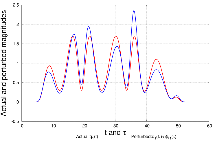
(a) Source 1

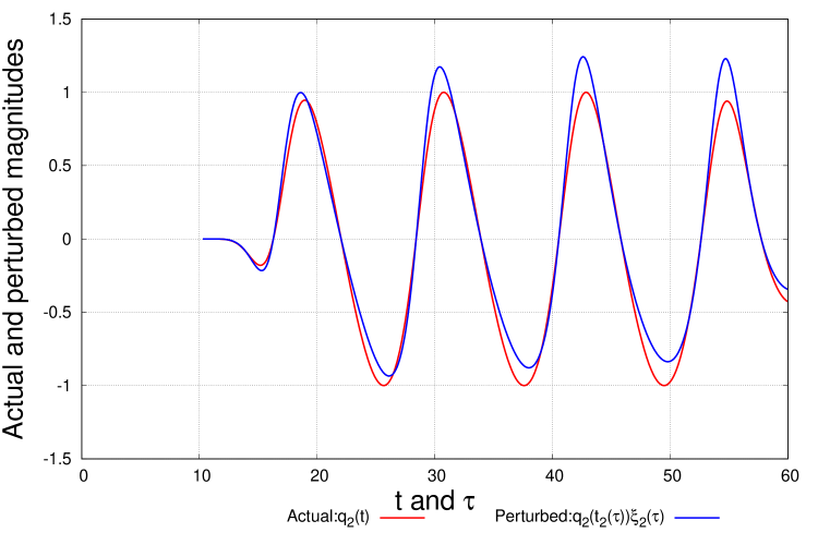
(b) Source 2

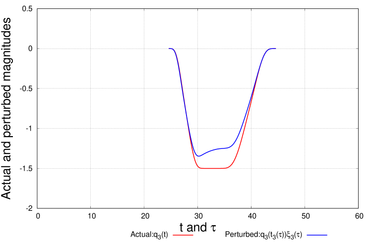
(c) Source 3

Figure 1: Behaviour of the actual and perturbed magnitude of point sources

Firstly, we discuss the identification of the number $K(\tau)$ of point sources. Figure 2(a) shows the behaviour of $|\det H_{k,0}(\tau)|$ in $0\leq\tau\leq T_{e}$ for $k=1,2,3,4$, and Figure 2(b) gives the behaviour of $|\det H_{k,0}(\tau)|$ at $\tau=10,\ 20$ and $40$ for observation data without noise. As we mentioned in Note 3.3, the results of Figure 2 show that we can not apply the condition (37) as it is for the identification of $K(\tau)$. However, we can observe that $|\det H_{k,0}(\tau)|$ has relatively large gap between $k=K(\tau)$ and $K(\tau)+1$. From this observation, we apply the following algorithm to identify $K(\tau)$:

Algorithm 4.1

Step 0.

Set positive parameters $\varepsilon_{0}$ and $\varepsilon_{G}$.

Step 1.

If $|\det H_{1,0}(\tau)|<\varepsilon_{0}$ and $|\det H_{1,0}(\tau)|>|\det H_{2,0}(\tau)|$, then $K(\tau)=0$.

Step 2.

If $|\det H_{1,0}(\tau)|>\varepsilon_{0}$ or $|\det H_{1,0}(\tau)|<|\det H_{2,0}(\tau)|$, then find largest number $k$ such that $|\det H_{k,0}(\tau)|/|\det H_{k-1,0}(\tau)|>\varepsilon_{G}$, and identify $K(\tau)=k$.

Figure 3 displays the identification results of $K(\tau)$ from observation data without noise and with 0.5% noise. Here, we set $\varepsilon_{0}=1.0\times 10^{-4}$ and $\varepsilon_{G}=2.5\times 10^{-2}$. From the result of Figure 3, we consider that Algorithm 4.1 works well even for observations with 0.5% noise. One can observe that identified $K(\tau)$ is smaller than the actual value around $\tau=12$ and $\tau=55$. We discuss a reason of these bad estimates later.

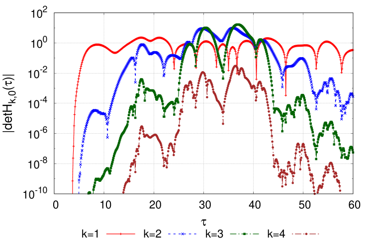
(a) behaviour of $|\det H_{k,0}(\tau)|$ for each $k$

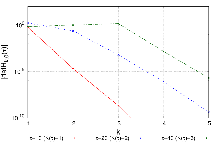
(b) behaviour of $|\det H_{k,0}(\tau)|$ for fixed $\tau$

Figure 2: Behaviour of $|\det H_{k,0}(\tau)|$ for observation data without noise: point source case.

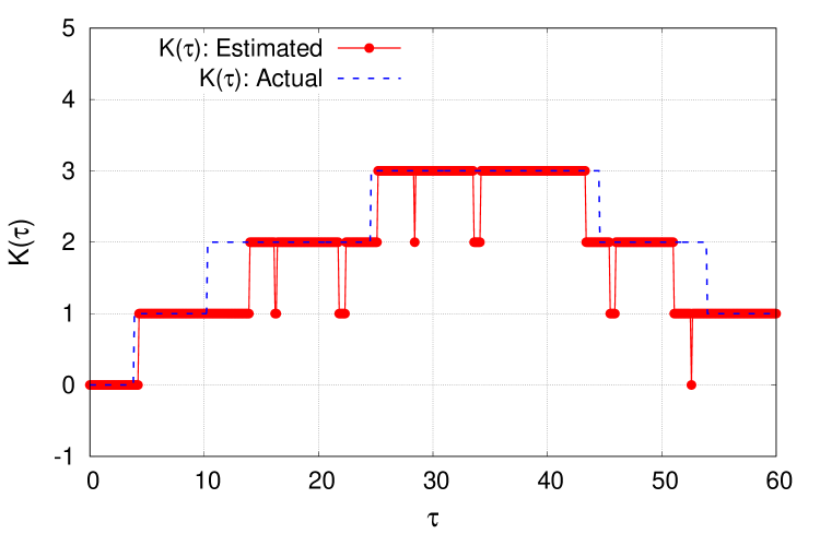
(a)

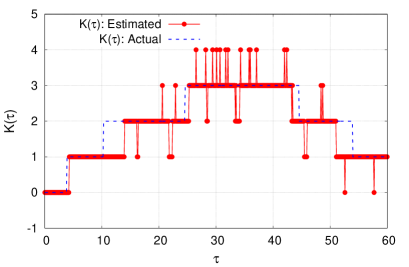
(b)

Figure 3: Behaviour of estimated number of point sources: (a) for observation data without noise, (b) with 0.5% noise.

Now, we show the reconstruction results of unknown parameters of moving point sources. Figures 4-7 display the reconstruction results of locations and magnitudes for observation data without noise, and with 0.1%, 0.5% and 1.0% noise. In these figures, we use the time variable $t$ for the horizontal axis by plotting $(t_{k}(\tau),\boldsymbol{p}_{k}(t_{k}(\tau)))$ and $(t_{k}(\tau),q_{k}(t_{k}(\tau)))$. In Table 4.1, we show the average errors of estimated locations and magnitudes for observations without noise, and with 0.1%, 0.5%, 1.0%, and 5.0% noise. Here we define

$$\mbox{average error of location }\boldsymbol{p}_{k}\equiv \displaystyle\sqrt{\frac{1}{|I|}\int_{I}|\widehat{\boldsymbol{p}}_{k}(t_{k}(\tau))-\boldsymbol{p}_{k}(t_{k}(\tau))|^{2}{\mathrm{d}}\tau},$$

$$\mbox{average error of magnitude }q_{k}\equiv \displaystyle\sqrt{\frac{1}{|I|}\int_{I}|\widehat{q}_{k}(t_{k}(\tau))-q_{k}(t_{k}(\tau))|^{2}{\mathrm{d}}\tau},$$

where $\widehat{\boldsymbol{p}}_{k}$ and $\widehat{q}_{k}$ denote the estimated location and magnitude of $k$-th point source, respectively, $I$ denotes the interval in which we evaluate the average error, and $|I|$ denotes the measure of $I$.

From results of Figures 4-7 and Table 4.1, we consider that our method works well if the noise of observation data is smaller than 0.5%. We can observe that if noise exceeds 1%, the influence of noise becomes unignorable in reconstruction results. Especially, estimations of magnitudes are highly affected by the observation noise. The reconstruction results become unreliable under the noise larger than 5%.

The average errors of estimated locations and magnitudes in each interval $3.9\leq\tau<10.2$ $10.2\leq\tau<24.6$ $24.6\leq\tau<44.6$ $44.6\leq\tau<54.0$ $54.0\leq\tau<60.0$ $(K(\tau)=1)$ $(K(\tau)=2)$ $(K(\tau)=3)$ $(K(\tau)=2)$ $(K(\tau)=1)$ (a) Without noise $\boldsymbol{p}_{1}$ $1.7E-2$ $3.9E-2$ $2.2E-2$ $8.1E-2$ $-$ $\boldsymbol{p}_{2}$ $-$ $3.6E-2$ $4.0E-2$ $3.1E-2$ $1.3E-1$ $\boldsymbol{p}_{3}$ $-$ $-$ $1.3E-2$ $-$ $-$ $q_{1}$ $1.3E-3$ $7.6E-2$ $3.2E-2$ $5.1E-2$ $-$ $q_{2}$ $-$ $1.1E-1$ $5.0E-2$ $3.2E-2$ $1.6E-2$ $q_{3}$ $-$ $-$ $2.5E-2$ $-$ $-$ (b) With $0.1\%$ noise $\boldsymbol{p}_{1}$ $1.7E-2$ $3.9E-2$ $2.3E-2$ $8.3E-2$ $-$ $\boldsymbol{p}_{2}$ $-$ $5.0E-2$ $3.2E-2$ $3.6E-2$ $1.5E-1$ $\boldsymbol{p}_{3}$ $-$ $-$ $3.8E-2$ $-$ $-$ $q_{1}$ $1.4E-2$ $8.0E-2$ $4.5E-2$ $5.2E-2$ $-$ $q_{2}$ $-$ $1.2E-1$ $5.6E-2$ $3.8E-2$ $2.7E-2$ $q_{3}$ $-$ $-$ $4.9E-2$ $-$ $-$ (c) With $0.5\%$ noise $\boldsymbol{p}_{1}$ $1.9E-2$ $4.7E-2$ $6.3E-2$ $1.9E-1$ $-$ $\boldsymbol{p}_{2}$ $-$ $2.2E-1$ $1.7E-1$ $4.1E-2$ $3.7E-2$ $\boldsymbol{p}_{3}$ $-$ $-$ $8.8E-2$ $-$ $-$ $q_{1}$ $8.1E-2$ $2.6E-1$ $4.7E-1$ $2.6E-1$ $-$ $q_{2}$ $-$ $2.1E-1$ $6.6E-1$ $1.4E-1$ $2.0E-1$ $q_{3}$ $-$ $-$ $2.1E-1$ $-$ $-$ (d) With $1.0\%$ noise $\boldsymbol{p}_{1}$ $1.6E-2$ $7.9E-2$ $8.8E-2$ $2.1E-1$ $-$ $\boldsymbol{p}_{2}$ $-$ $2.7E-1$ $2.4E-1$ $5.9E-2$ $1.1E-1$ $\boldsymbol{p}_{3}$ $-$ $-$ $2.5E-1$ $-$ $-$ $q_{1}$ $1.5E-1$ $5.2E-1$ $1.2E+0$ $4.1E-1$ $-$ $q_{2}$ $-$ $2.7E-1$ $1.0E+0$ $4.5E-1$ $6.0E-1$ $q_{3}$ $-$ $-$ $7.3E-1$ $-$ $-$ (e) With $5.0\%$ noise $\boldsymbol{p}_{1}$ $5.7E-2$ $2.1E-1$ $2.2E-1$ $7.1E-1$ $-$ $\boldsymbol{p}_{2}$ $-$ $6.0E-1$ $5.0E-1$ $2.5E-1$ $1.9E-1$ $\boldsymbol{p}_{3}$ $-$ $-$ $2.9E-1$ $-$ $-$ $q_{1}$ $1.9E+0$ $3.4E+0$ $3.9E+0$ $1.6E+0$ $-$ $q_{2}$ $-$ $2.1E+0$ $3.7E+0$ $2.9E+0$ $3.6E+0$ $q_{3}$ $-$ $-$ $3.8E+0$ $-$ $-$

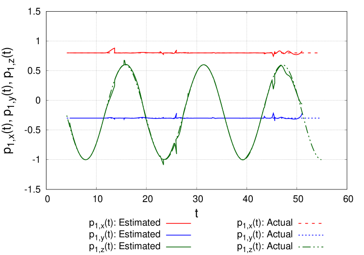
(a) location of source 1

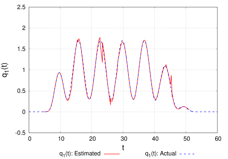
(b) magnitude of source 1

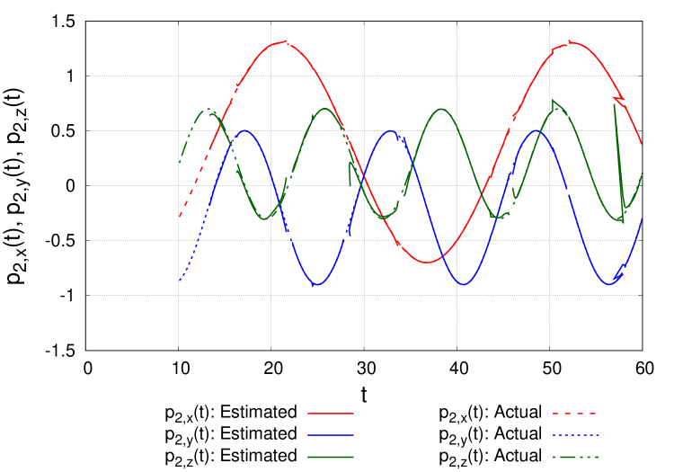
(c) location of source 2

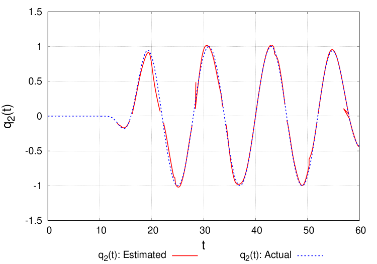
(d) magnitude of source 2

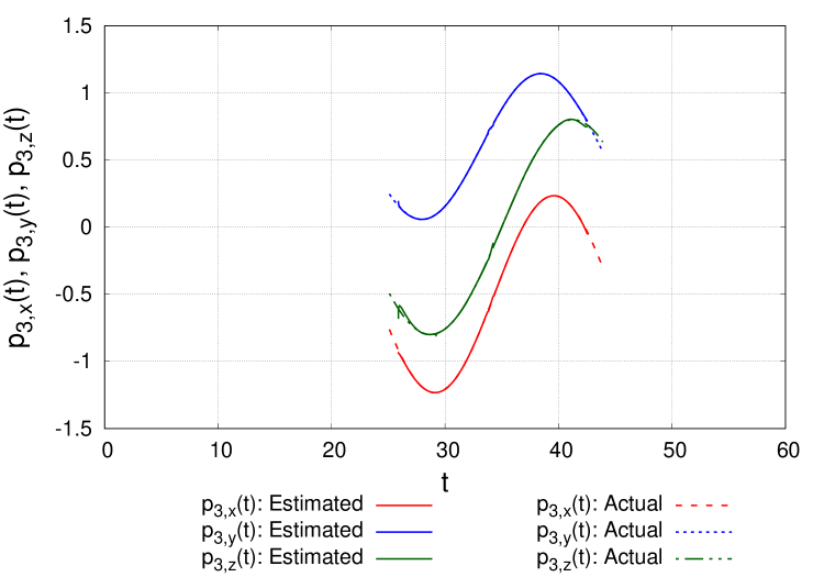
(e) location of source 3

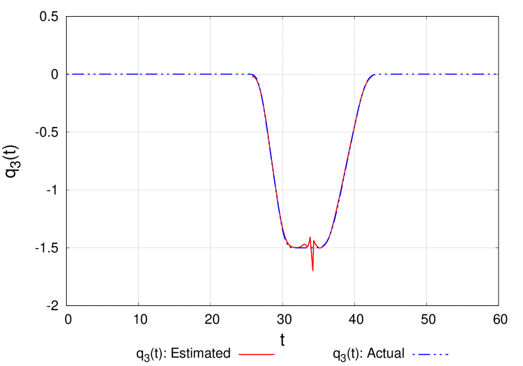
(f) magnitude of source 3

Figure 4: Estimated locations and magnitudes of point sources for observation data without noise.

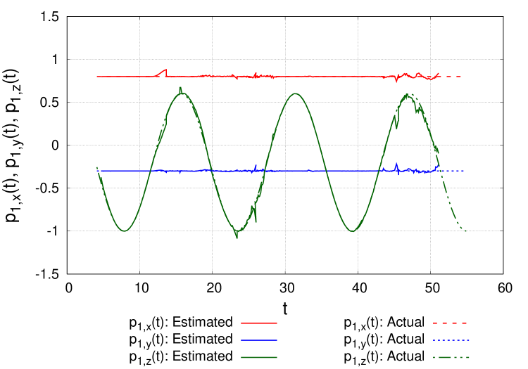
(a) location of source 1

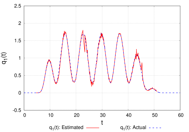
(b) magnitude of source 1

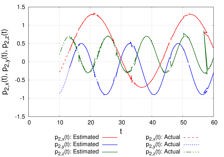
(c) location of source 2

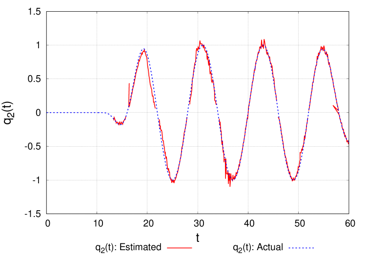
(d) magnitude of source 2

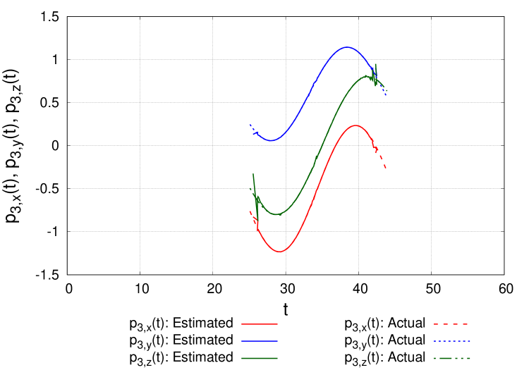
(e) location of source 3

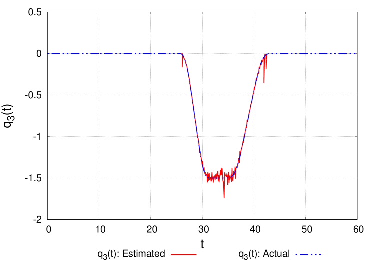
(f) magnitude of source 3

Figure 5: Estimated locations and magnitudes of point sources for observation data with 0.1% noise.

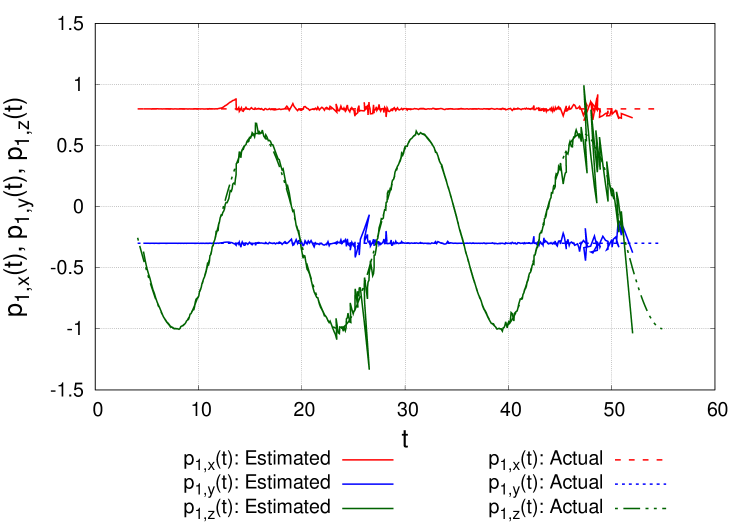
(a) location of source 1

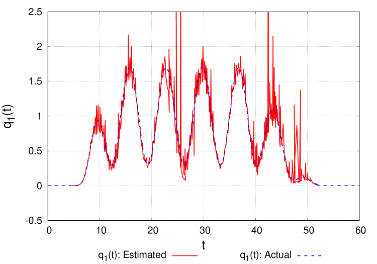
(b) magnitude of source 1

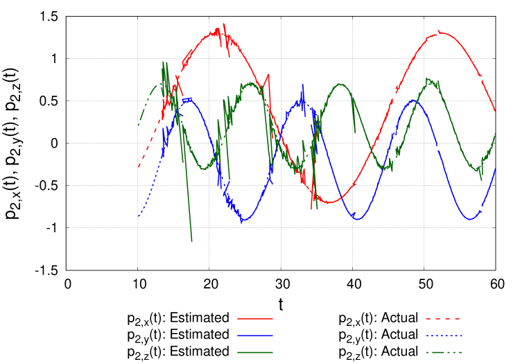
(c) location of source 2

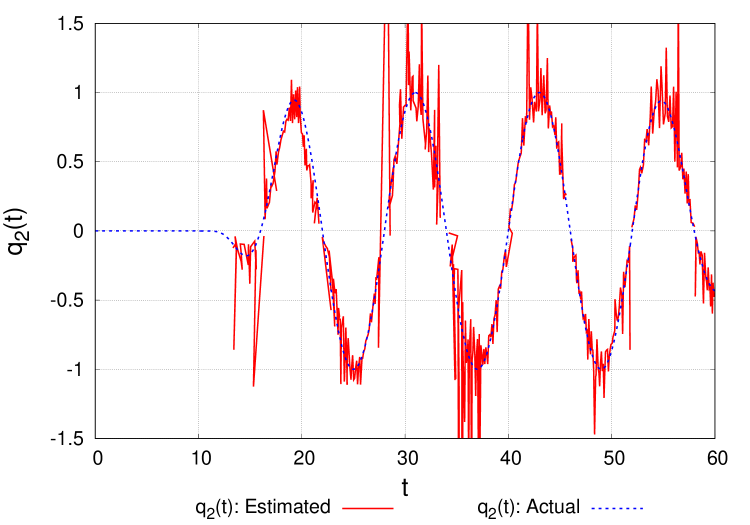
(d) magnitude of source 2

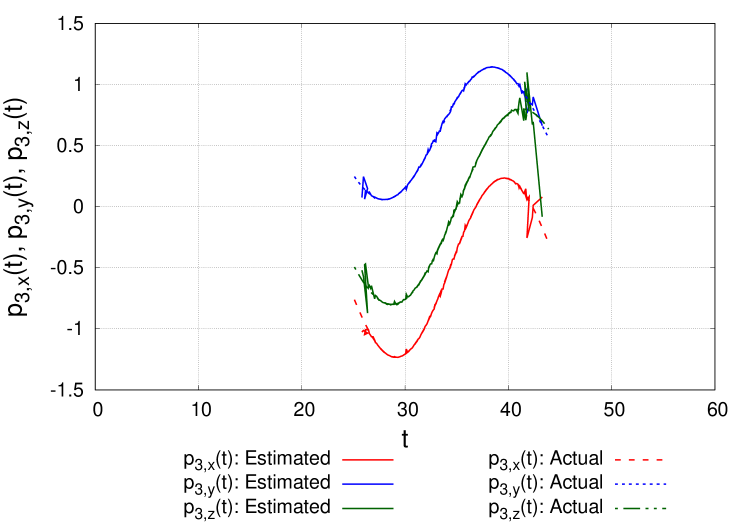
(e) location of source 3

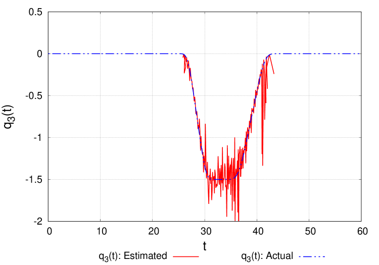
(f) magnitude of sources 3

Figure 6: Estimated locations and magnitudes of point sources for observation data with 0.5% noise.

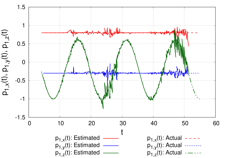
(a) location of source 1

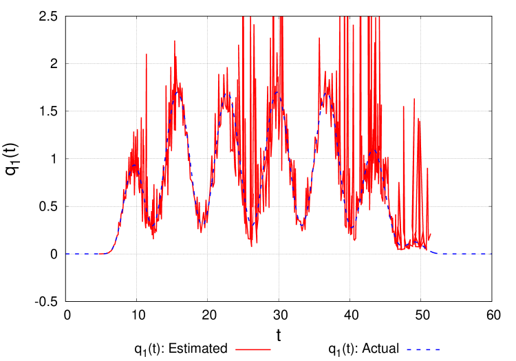
(b) magnitude of source 1

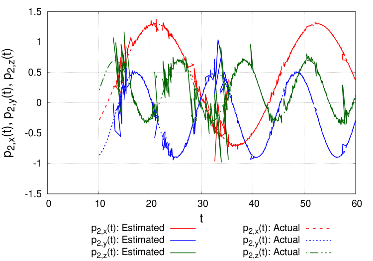
(c) location of source 2

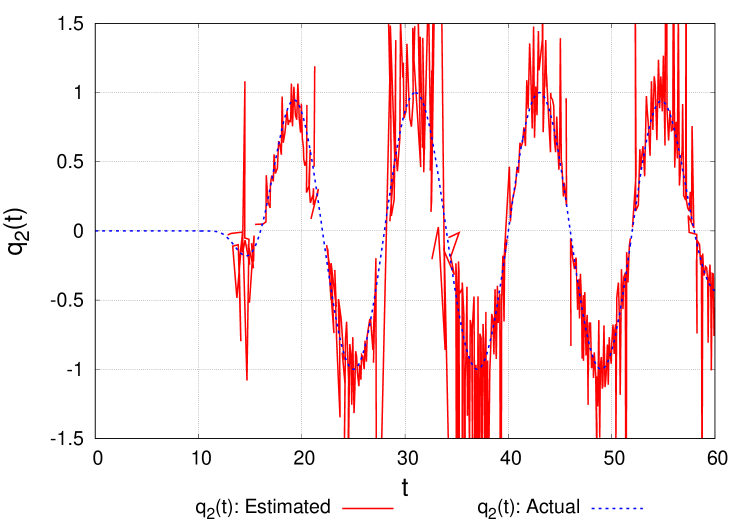
(d) magnitude of source 2

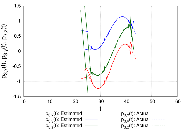
(e) location of source 3

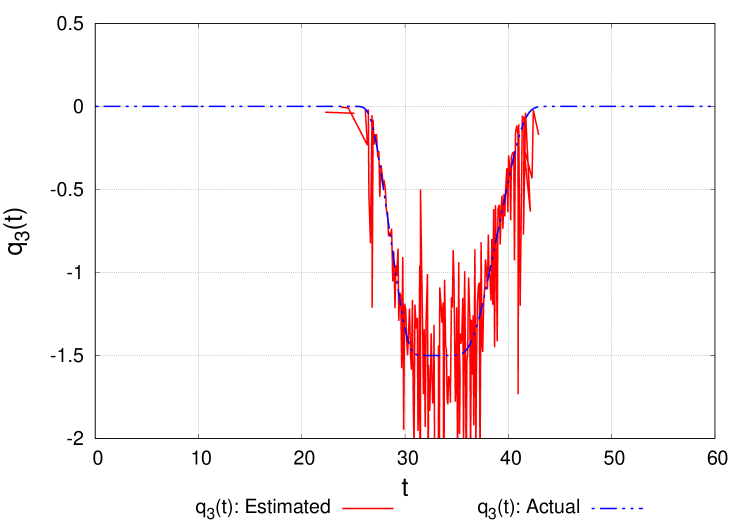
(f) magnitude of source 3

Figure 7: Estimated locations and magnitudes of point sources for observation data with 1.0% noise.

We can find that the reconstruction of location becomes bad for the source with small magnitude, e.g. the result of source 2 around $t=12$ in Figures 6(b) and 7(b), but we consider that these results are reasonable. We can also find bad reconstruction results due to small magnitude for source 2 in the interval $54.0\leq\tau<60.0$ for the observation without noise and 1.0% noise in Table 4.1, and bad identification of $K(\tau)$ around $\tau=12$ and $\tau=53$ in Figure 3(b).

Note 4.1. In Table 4.1, the error of $\boldsymbol{p}_{2}$ in the interval $54.0\leq\tau\leq 60.0$ is concentrated in $57.6\leq\tau\leq 57.8$ where $q_{2}(t_{2}(\tau))\simeq 0$. Except of these bad estimates, the average error of $\boldsymbol{p}_{2}$ in $54.0\leq\tau<60.0$ becomes $1.56E-2$ for the case without noise and $1.45E-2$ for the case with 0.1% noise.

In Figures 6 and 7, we can also find bad reconstruction results even for large magnitudes of point sources, e.g. results for sources 2 and 3 at around $t=30$. To discuss the reason of these bad estimates, we display the behaviour of distances between each two point sources in Figure 8. The results of Figures 6-8 suggest that if the arangement of point sources is well separated, then our method works well and gives good reconstruction results, however, as arrangement of point sources becomes closer, then it becomes more difficult to distinguish these sources, and our method gives bad estimations.

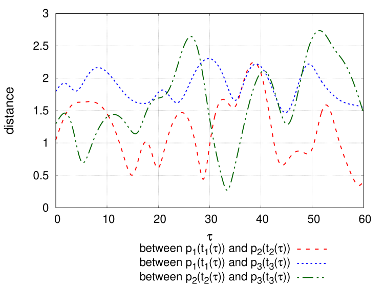
(a)

Figure 8: Behaviour of the distances between each two point sources.

In Figure 3(b), we can find many wrong identification results of $K(\tau)$, especially, in $25\leq\tau\leq 38$ where $K(\tau)$ is identified as 4. However, the absolute value of magnitude of reconstructed 4th source is very small ($<0.01$) comparing to other sources, and so the 4th source can be recognised as ‘noises’ or ‘ghosts’.

Note 4.2. Since our reconstruction procedure works at every moment $\tau$, we have to identify whether the point source reconstructed at the moment $\tau$ belongs to which source reconstructed at the previous moment $\tau-\Delta\tau$, especially, when $K(\tau)$ changes. To solve this problem, we measure distances between the reconstructed sources at moments $\tau$ and $\tau-\Delta\tau$, and identify as the same source which has the minimum distance.

Throughout of the numerical results, we can observe that the observation noise affects to the estimation of magnitudes more heavily than the one of locations. This phenomena is mainly caused by the estimation of perturbation term $\xi_{k}(t_{k}(\tau))$. As an alternative method, we apply Step 4’ in Note 3.5 to obtain $dp_{k,z}(t_{k}(\tau))/d\tau$, and compare to results by Step 4. Here, we apply the central differences

$$\frac{dp_{k,z}(t_{k}(\tau))}{d\tau}\sim\frac{p_{k,z}(\tau+\Delta\tau)-p_{k,z}(\tau-\Delta\tau)}{2\cdot\Delta\tau}.$$

to estimate $dp_{k,z}(t_{k}(\tau))/d\tau$, where $p_{k,z}(t_{k}(\tau))$ is obtained in Step 3. Table 4.1 shows the average errors of estimated magnitudes using Step 4’ instead of Step 4. Comparing Tables 4.1 and 4.1, the errors are almost the same in both methods for the case where the observation noise is smaller than 0.5%. Hence we consider that both method can be used as an alternative if the noise is small.

The average errors of estimated magnitudes in each interval using Step 4’ instead of Step 4. $3.9\leq\tau<10.2$ $10.2\leq\tau<24.6$ $24.6\leq\tau<44.6$ $44.6\leq\tau<54.0$ $54.0\leq\tau<60.0$ $(K(\tau)=1)$ $(K(\tau)=2)$ $(K(\tau)=3)$ $(K(\tau)=2)$ $(K(\tau)=1)$ (a) Without noise $q_{1}$ $1.8E-2$ $1.5E-1$ $9.5E-2$ $8.5E-2$ $-$ $q_{2}$ $-$ $1.5E-2$ $4.3E-2$ $5.5E-2$ $5.0E-2$ $q_{3}$ $-$ $-$ $3.4E-2$ $-$ $-$ (b) With $0.1\%$ noise $q_{1}$ $1.8E-2$ $1.6E-1$ $9.6E-2$ $9.0E-2$ $-$ $q_{2}$ $-$ $5.0E-2$ $6.0E-2$ $5.8E-2$ $5.4E-2$ $q_{3}$ $-$ $-$ $4.0E-2$ $-$ $-$ (c) With $0.5\%$ noise $q_{1}$ $3.6E-2$ $2.6E-1$ $1.5E-1$ $1.6E-1$ $-$ $q_{2}$ $-$ $2.0E-1$ $2.6E-1$ $8.8E-2$ $8.8E-2$ $q_{3}$ $-$ $-$ $9.3E-2$ $-$ $-$ (d) With $1.0\%$ noise $q_{1}$ $5.0E-2$ $5.1E-1$ $2.9E-1$ $2.4E-1$ $-$ $q_{2}$ $-$ $4.2E-1$ $6.0E-1$ $1.4E-1$ $1.3E-1$ $q_{3}$ $-$ $-$ $1.8E-1$ $-$ $-$ (e) With $5.0\%$ noise $q_{1}$ $2.5E-1$ $1.2E+0$ $8.0E-1$ $5.5E-1$ $-$ $q_{2}$ $-$ $1.6E+0$ $1.8E+0$ $6.2E-1$ $7.0E-1$ $q_{3}$ $-$ $-$ $6.2E-1$ $-$ $-$

4.2 Reconstruction of moving dipole sources

Next, we demonstrate numerical experiments for reconstruction of moving dipole sources. We consider the case where three dipole sources move in the domain $\Omega$. The locations of dipoles are arranged as same as the previous example, and moments of dipoles change as follows:

source 1.

${\boldsymbol{m}}_{1}(t)=(m_{1,x}(t),\ m_{1,y}(t),\ 0)$ where

$$m_{1,x}(t) =\left\{\begin{array}[]{ll}0,&0\leq t<2,\\[4.30554pt] \displaystyle\frac{1}{2}\eta\left(\frac{t-2}{7}\right)\cdot\cos\left(\frac{2\pi t}{10}\right),&2\leq t<9,\\[12.91663pt] \displaystyle\frac{1}{2}\cos\left(\frac{2\pi t}{10}\right),&9\leq t<32,\\[12.91663pt] \displaystyle\frac{1}{2}\left(1-\eta\left(\frac{t-32}{9}\right)\right)\cdot\cos\left(\frac{2\pi t}{10}\right),&32\leq t<41,\\[12.91663pt] 0,&41\leq t\leq 70,\end{array}\right.$$

$$m_{1,y}(t) =\left\{\begin{array}[]{ll}0,&0\leq t<2,\\[4.30554pt] \displaystyle\frac{1}{2}\eta\left(\frac{t-2}{7}\right)\cdot\sin\left(\frac{2\pi t}{10}\right),&2\leq t<9,\\[12.91663pt] \displaystyle\frac{1}{2}\sin\left(\frac{2\pi t}{10}\right),&9\leq t<32,\\[12.91663pt] \displaystyle\frac{1}{2}\left(1-\eta\left(\frac{t-32}{9}\right)\right)\cdot\sin\left(\frac{2\pi t}{10}\right),&32\leq t<41,\\[12.91663pt] 0,&41\leq t\leq 70,\end{array}\right.$$

source 2.

${\boldsymbol{m}}_{2}(t)=(m_{2,x}(t),\ m_{2,y}(t),\ 0)$ where

$$m_{2,x}(t) =\left\{\begin{array}[]{ll}0,&0\leq t<7,\\[8.61108pt] \displaystyle\eta\left(\frac{t-7}{5}\right)\cdot\left(\frac{3}{5}-\frac{1}{5}\cos\left(\frac{2\pi(t-7)}{15}\right)\right)\cdot\sin\left(-\frac{2\pi t}{11}\right),&7\leq t<12,\\[12.91663pt] \displaystyle\left(\frac{3}{5}-\frac{1}{5}\cos\left(\frac{2\pi(t-7)}{15}\right)\right)\cdot\sin\left(-\frac{2\pi t}{11}\right),&12\leq t\leq 70,\end{array}\right.$$

$$m_{2,y}(t) =\left\{\begin{array}[]{ll}0,&0\leq t<7,\\[8.61108pt] \displaystyle\eta\left(\frac{t-7}{5}\right)\cdot\left(\frac{3}{5}-\frac{1}{5}\cos\left(\frac{2\pi(t-7)}{15}\right)\right)\cdot\cos\left(-\frac{2\pi t}{11}\right),&7\leq t<12,\\[12.91663pt] \displaystyle\left(\frac{3}{5}-\frac{1}{5}\cos\left(\frac{2\pi(t-7)}{15}\right)\right)\cdot\cos\left(-\frac{2\pi t}{11}\right),&12\leq t\leq 70.\end{array}\right.$$

source 3.

${\boldsymbol{m}}_{3}(t)=(m_{3,x}(t),\ m_{3,y}(t),\ 0)$ where

$$m_{3,x}(t) =\left\{\begin{array}[]{ll}0,&0\leq t<18,\\[4.30554pt] \displaystyle\eta\left(\frac{t-18}{8}\right)\cdot\cos\left(\frac{2\pi t}{8}\right),&18\leq t<26,\\[12.91663pt] \displaystyle\cos\left(\frac{2\pi t}{8}\right),&26\leq t<45,\\[12.91663pt] \displaystyle\left(1-\eta\left(\frac{t-45}{9}\right)\right)\cdot\cos\left(\frac{2\pi t}{8}\right),&45\leq t<54,\\[12.91663pt] 0,&54\leq t\leq 70,\end{array}\right.$$

$$m_{3,y}(t) =\left\{\begin{array}[]{ll}0,&0\leq t<18,\\[4.30554pt] \displaystyle\eta\left(\frac{t-18}{8}\right)\cdot\sin\left(\frac{2\pi t}{8}\right),&18\leq t<26,\\[12.91663pt] \displaystyle\sin\left(\frac{2\pi t}{8}\right),&26\leq t<45,\\[12.91663pt] \displaystyle\left(1-\eta\left(\frac{t-45}{9}\right)\right)\cdot\sin\left(\frac{2\pi t}{8}\right),&45\leq t<54,\\[12.91663pt] 0,&54\leq t\leq 70.\end{array}\right.$$

Hence $K(\tau)$ changes as

$$K(\tau)=\left\{\begin{array}[]{ll}0,&0\leq\tau<2.4,\\[4.30554pt] 1,&2.4\leq\tau<6.8,\ \ 54.8\leq\tau\leq 70.0,\\[4.30554pt] 2,&6.8\leq\tau<17.3,\ \ 40.2\leq\tau<54.8,\\[4.30554pt] 3,&17.3\leq\tau<40.2.\end{array}\right.$$

We note that $\boldsymbol{m}_{k}\in C^{4}([0,70]),\ k=1,2,3$.

We first discuss the identification of the number $K(\tau)$ of dipoles. Figure 9 shows the behaviour of $|\det H_{k,1}(\tau)|$ for $0\leq\tau\leq T_{e}$. The behaviour of $|\det H_{k,1}(\tau)|$ is quite similar as for the one of $|\det H_{k,0}(\tau)|$ for point sources in Figure 2, and hence we apply Algorithm 4.1 for the identification of $K(\tau)$ using $H_{k,1}(\tau)$ instead of $H_{k,0}(\tau)$. Figure 10 displays the identification results of $K(\tau)$ from observations without noise and with 0.5% noise. Here, we set the parameters $\varepsilon_{0}=1.0\times 10^{-4}$ and $\varepsilon_{G}=2.5\times 10^{-2}$ as same as for moving point sources. From the result of Figure 10, we consider Algorithm 4.1 also works well for the identification of the number of moving dipole sources.

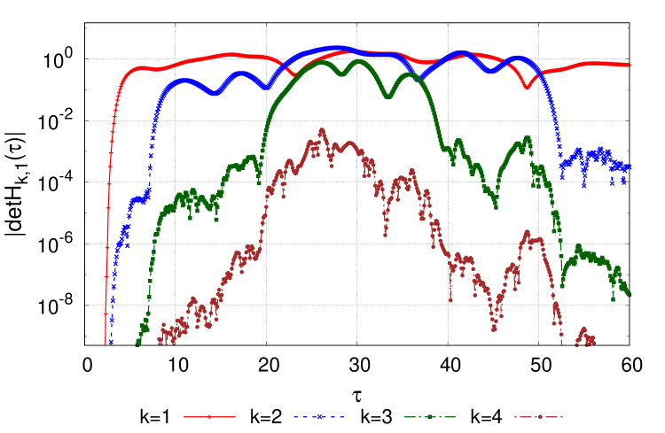
(a)

Figure 9: Behaviour of $|\det H_{k,1}(\tau)|$ for observation data without noise: dipole source case.

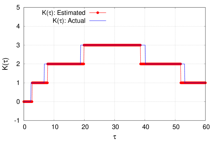
(a)

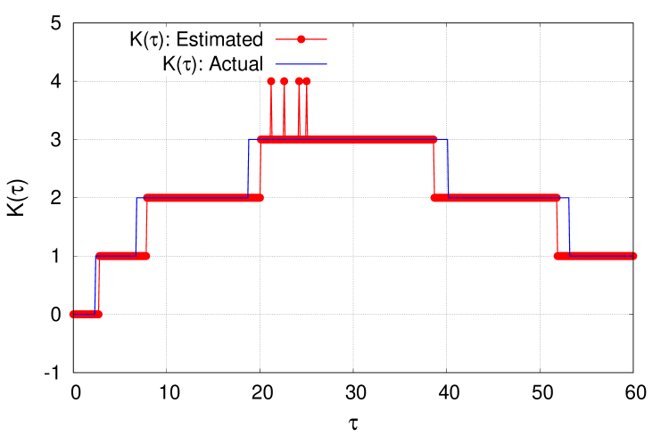
(b)

Figure 10: Behaviour of estimated number of dipole sources: (a) for observation data without noise, (b) with $0.5\%$ noise.

Next, we show the reconstruction results for locations and moments of dipole sources. Figures 11-14 display the reconstruction results from observations without noise, and with 0.1%, 0.5% and 1.0% noise. Also in Table 4.2, we show the average errors of estimated locations and moments. Here we define the average error of each moment by

$$\mbox{average error of moment }\boldsymbol{m}_{k}\equiv\displaystyle\sqrt{\frac{1}{|I|}\int_{I}|\widehat{\boldsymbol{m}}_{k}(t_{k}(\tau))-\boldsymbol{m}_{k}(t_{k}(\tau))|^{2}{\mathrm{d}}\tau},$$

where $\widehat{\boldsymbol{m}}_{k}$ denotes the estimated moment of $k$-th dipole source. Same as for the reconstruction of point sources, our method works well if the noise of observation data is smaller than 0.5%. The noise of observation becomes 1%, the influence of noise becomes unignorable, and our method can not give reliable estimates under 5% noise. We can see that observation noises affect to the estimations of moments more heavily than the reconstruction of locations. The reconstruction result also becomes bad when the norm of moment is small, and when the arrangement of dipoles is clustered.

The average errors of estimated locations and moments in each interval $2.4\leq\tau<6.8$ $6.8\leq\tau<17.3$ $17.3\leq\tau<40.2$ $40.2\leq\tau<54.8$ $54.8\leq\tau<60.0$ $(K(\tau)=1)$ $(K(\tau)=2)$ $(K(\tau)=3)$ $(K(\tau)=2)$ $(K(\tau)=1)$ (a) Without noise $\boldsymbol{p}_{1}$ $5.6E-2$ $6.9E-3$ $3.7E-2$ $-$ $-$ $\boldsymbol{p}_{2}$ $-$ $8.4E-3$ $2.5E-2$ $4.3E-3$ $3.2E-3$ $\boldsymbol{p}_{3}$ $-$ $-$ $2.0E-2$ $2.6E-2$ $-$ $\boldsymbol{m}_{1}$ $1.6E-3$ $3.6E-2$ $6.7E-2$ $-$ $-$ $\boldsymbol{m}_{2}$ $-$ $2.2E-2$ $5.9E-2$ $4.0E-2$ $2.7E-2$ $\boldsymbol{m}_{3}$ $-$ $-$ $2.8E-2$ $1.3E-2$ $-$ (b) With $0.1\%$ noise $\boldsymbol{p}_{1}$ $5.5E-2$ $8.2E-3$ $5.4E-2$ $-$ $-$ $\boldsymbol{p}_{2}$ $-$ $1.5E-2$ $4.3E-2$ $4.6E-3$ $4.1E-3$ $\boldsymbol{p}_{3}$ $-$ $-$ $3.3E-2$ $2.9E-2$ $-$ $\boldsymbol{m}_{1}$ $5.1E-3$ $3.9E-2$ $7.1E-2$ $-$ $-$ $\boldsymbol{m}_{2}$ $-$ $3.2E-2$ $1.5E-1$ $4.7E-2$ $5.6E-2$ $\boldsymbol{m}_{3}$ $-$ $-$ $3.4E-2$ $2.1E-2$ $-$ (c) With $0.5\%$ noise $\boldsymbol{p}_{1}$ $5.5E-2$ $2.6E-2$ $2.1E-1$ $-$ $-$ $\boldsymbol{p}_{2}$ $-$ $6.2E-2$ $1.7E-1$ $8.6E-3$ $1.5E-2$ $\boldsymbol{p}_{3}$ $-$ $-$ $1.4E-1$ $7.7E-2$ $-$ $\boldsymbol{m}_{1}$ $2.0E-2$ $1.1E-1$ $3.4E-1$ $-$ $-$ $\boldsymbol{m}_{2}$ $-$ $1.6E-1$ $6.9E-1$ $1.4E-1$ $5.6E-1$ $\boldsymbol{m}_{3}$ $-$ $-$ $4.4E-1$ $6.2E-2$ $-$ (d) With $1.0\%$ noise $\boldsymbol{p}_{1}$ $1.0E-1$ $5.3E-2$ $2.7E-1$ $-$ $-$ $\boldsymbol{p}_{2}$ $-$ $1.9E-1$ $2.5E-1$ $2.2E-2$ $3.2E-2$ $\boldsymbol{p}_{3}$ $-$ $-$ $1.7E-1$ $2.1E-1$ $-$ $\boldsymbol{m}_{1}$ $4.0E-2$ $6.1E-1$ $9.2E-1$ $-$ $-$ $\boldsymbol{m}_{2}$ $-$ $1.2E+0$ $9.0E-1$ $8.4E-1$ $2.2E+0$ $\boldsymbol{m}_{3}$ $-$ $-$ $5.9E-1$ $1.6E-1$ $-$ (e) With $5.0\%$ noise $\boldsymbol{p}_{1}$ $9.5E-2$ $2.7E-1$ $6.8E-1$ $-$ $-$ $\boldsymbol{p}_{2}$ $-$ $4.5E-1$ $4.4E-1$ $1.1E-1$ $1.3E-1$ $\boldsymbol{p}_{3}$ $-$ $-$ $3.5E-1$ $3.3E-1$ $-$ $\boldsymbol{m}_{1}$ $1.2E+0$ $2.2E+0$ $2.9E+0$ $-$ $-$ $\boldsymbol{m}_{2}$ $-$ $3.2E+0$ $2.9E+0$ $2.5E+0$ $2.7E+0$ $\boldsymbol{m}_{3}$ $-$ $-$ $2.3E+0$ $1.7E+0$ $-$

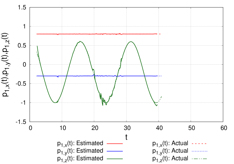
(a) location of source 1

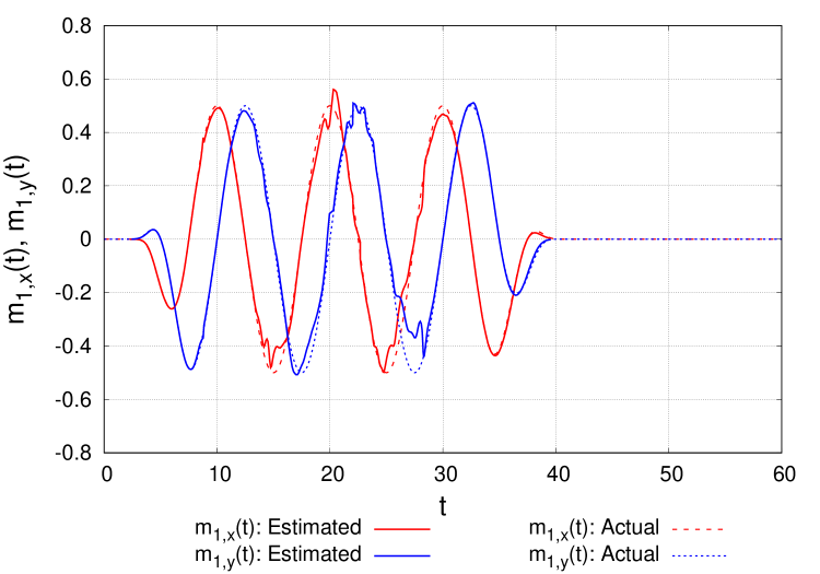
(b) moment of sources 1

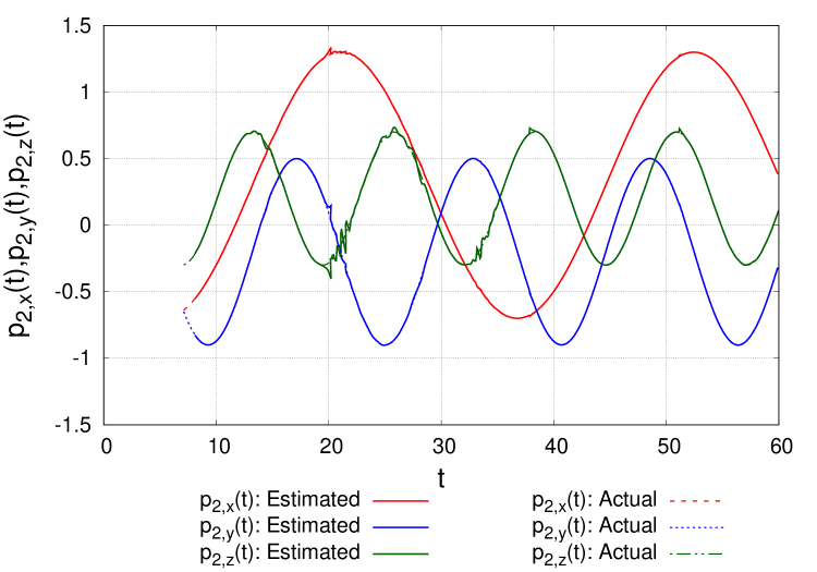
(c) location of source 2

(d) moment of source 2

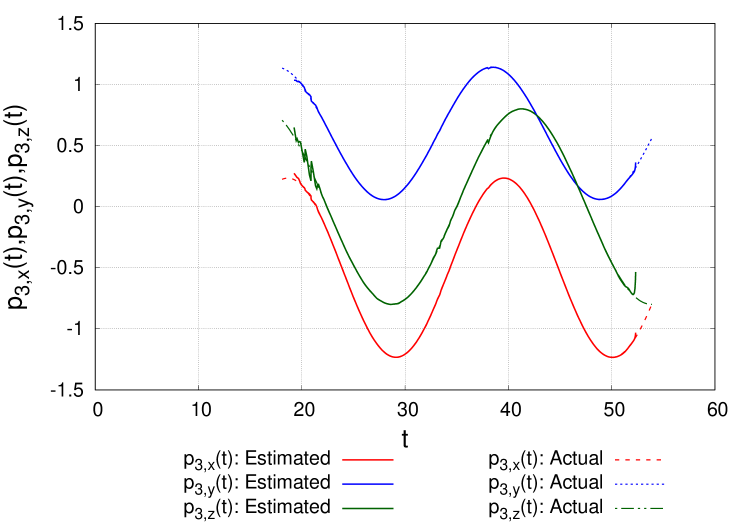
(e) location of source 3

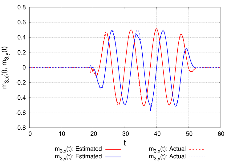
(f) moment of source 3

Figure 11: Estimated locations and moments of dipole sources for observation data without noise.

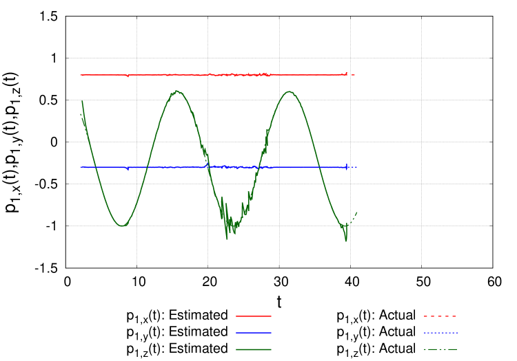
(a) location of source 1

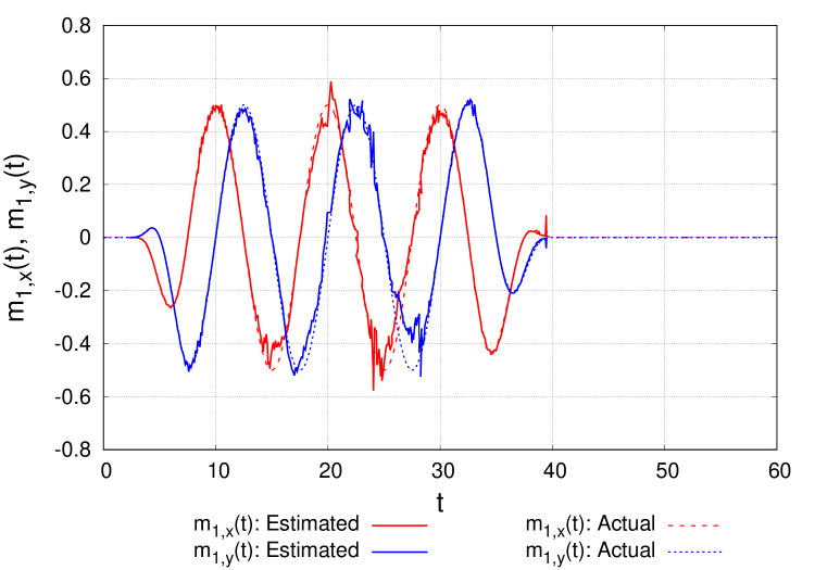
(b) moment of sources 1

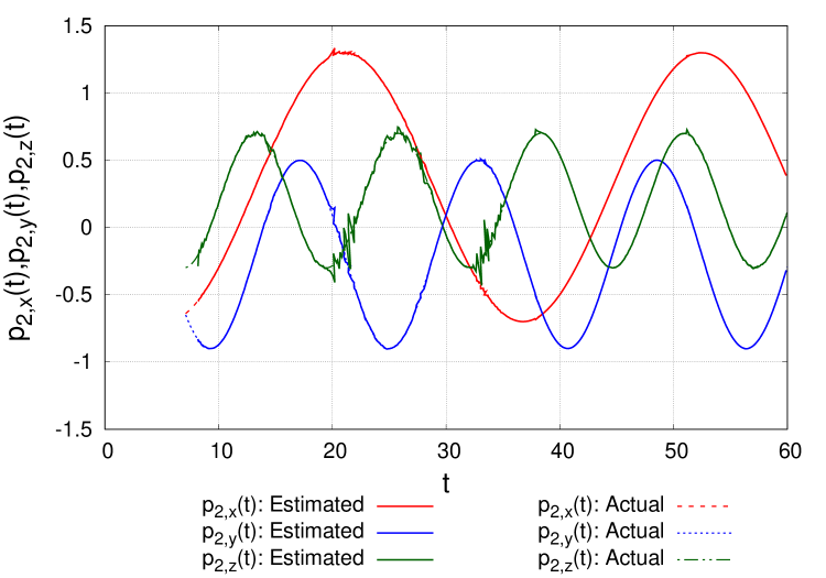
(c) location of source 2

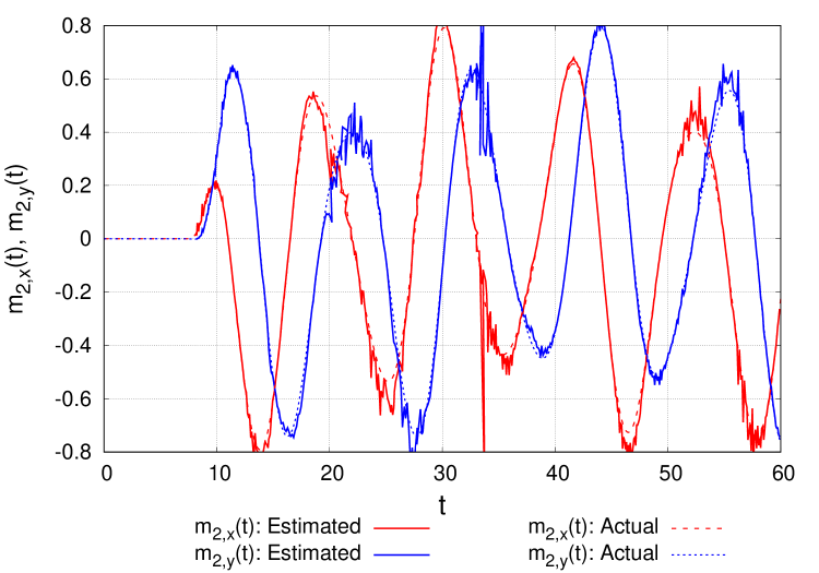
(d) moment of source 2

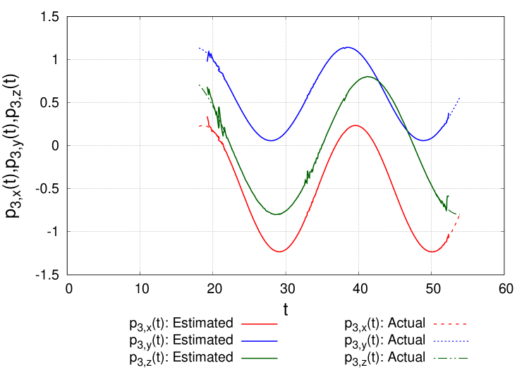
(e) location of source 3

(f) moment of source 3

Figure 12: Estimated locations and moments of dipole sources for observation data with 0.1% noise.

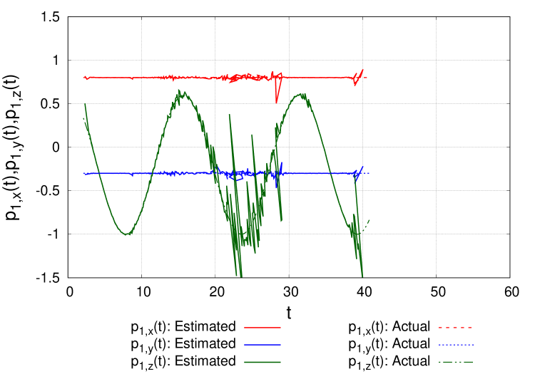
(a) location of source 1

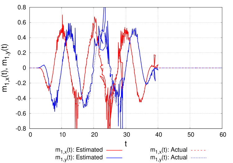
(b) moment of sources 1

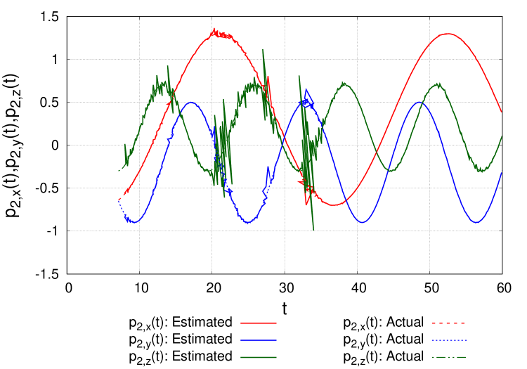
(c) location of source 2

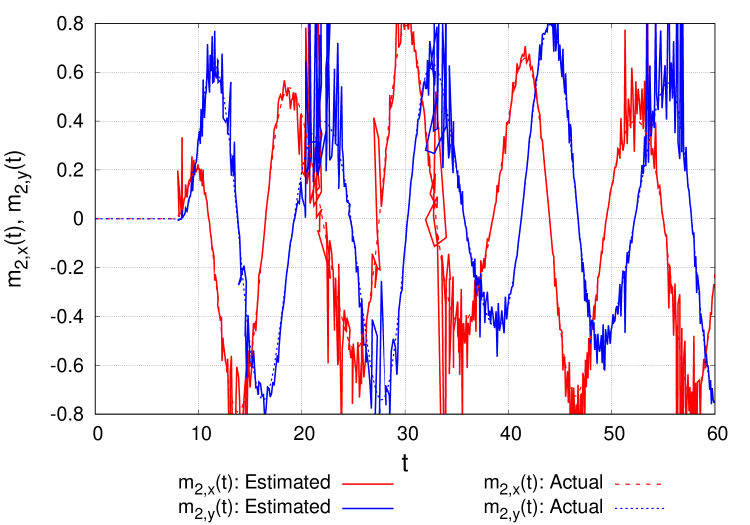
(d) moment of source 2

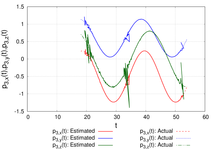
(e) location of source 3

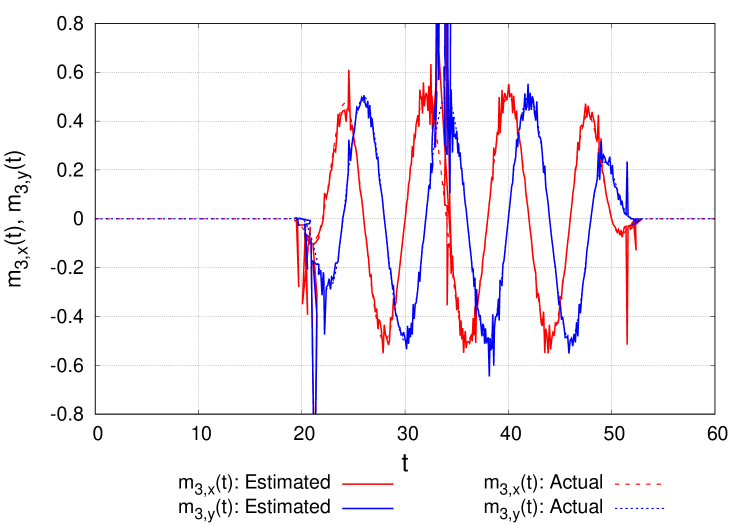
(f) moment of source 3

Figure 13: Estimated locations and moments of dipole sources for observation data with 0.5% noise.

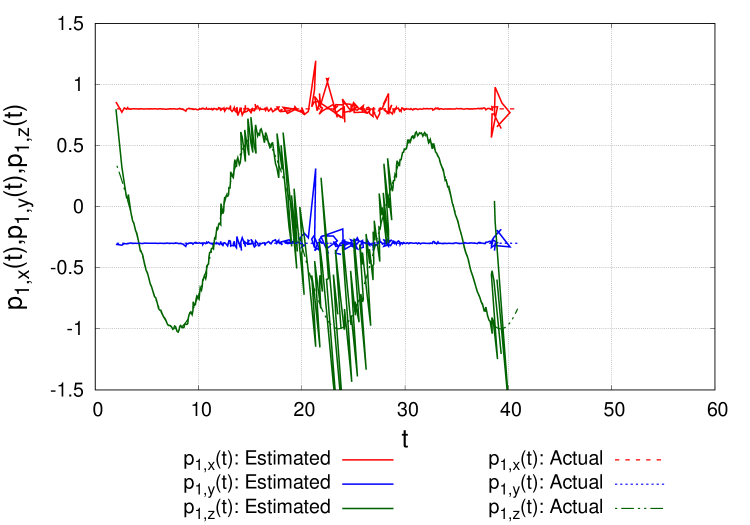
(a) location of source 1

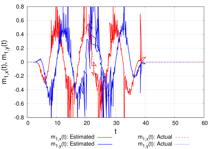
(b) moment of sources 1

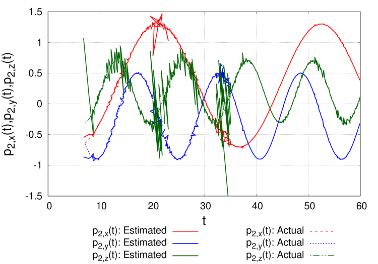
(c) location of source 2

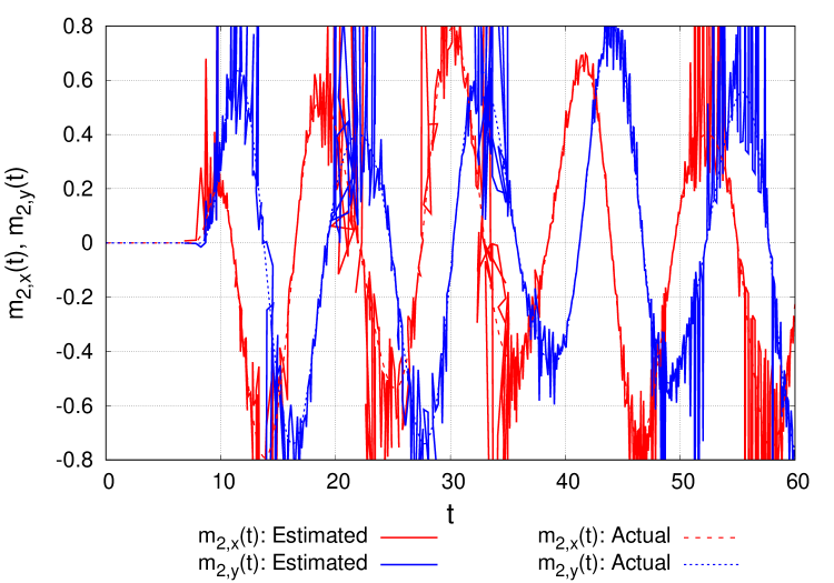
(d) moment of source 2

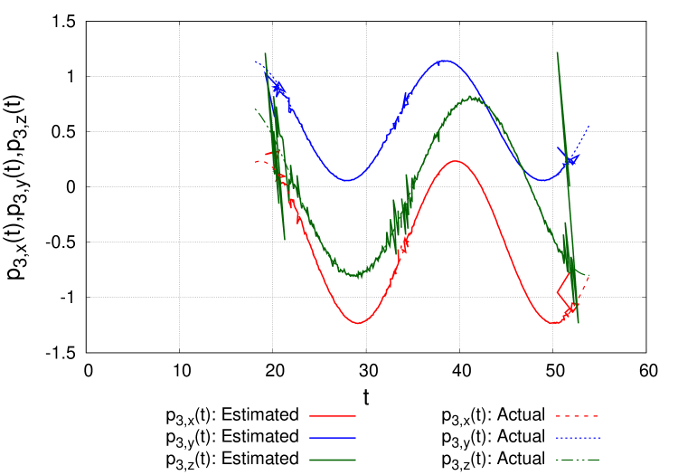
(e) location of source 3

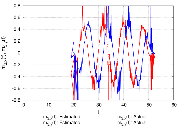
(f) moment of source 3

Figure 14: Estimated locations and moments of dipole sources for observation data with 1.0% noise.

Finally, we show the average of error of estimated moments by using Step 4’ instead of Step 4 in Table 4.2. As same as for moving point source, the errors of estimation results are almost the same in both methods if observation noise is smaller than 1.0%.

The average errors of estimated moments in each interval using Step 4’ instead of Step 4. $2.4\leq\tau<6.8$ $6.8\leq\tau<17.3$ $17.3\leq\tau<40.2$ $40.2\leq\tau<54.8$ $54.8\leq\tau<60.0$ $(K(\tau)=1)$ $(K(\tau)=2)$ $(K(\tau)=3)$ $(K(\tau)=2)$ $(K(\tau)=1)$ (a) Without noise $\boldsymbol{m}_{1}$ $1.7E-2$ $2.4E-2$ $1.4E-1$ $-$ $-$ $\boldsymbol{m}_{2}$ $-$ $6.0E-2$ $8.8E-2$ $3.1E-2$ $2.4E-2$ $\boldsymbol{m}_{3}$ $-$ $-$ $2.6E-2$ $1.4E-2$ $-$ (b) With $0.1\%$ noise $\boldsymbol{m}_{1}$ $1.8E-2$ $2.8E-2$ $2.1E-2$ $-$ $-$ $\boldsymbol{m}_{2}$ $-$ $8.0E-2$ $1.6E-1$ $3.3E-2$ $3.1E-2$ $\boldsymbol{m}_{3}$ $-$ $-$ $4.9E-2$ $1.5E-2$ $-$ (c) With $0.5\%$ noise $\boldsymbol{m}_{1}$ $2.1E-2$ $8.8E-2$ $8.5E-1$ $-$ $-$ $\boldsymbol{m}_{2}$ $-$ $4.1E-1$ $7.2E-1$ $4.7E-2$ $9.1E-2$ $\boldsymbol{m}_{3}$ $-$ $-$ $3.3E-1$ $2.4E-2$ $-$ (d) With $1.0\%$ noise $\boldsymbol{m}_{1}$ $3.6E-2$ $2.0E-1$ $1.1E+0$ $-$ $-$ $\boldsymbol{m}_{2}$ $-$ $8.4E-1$ $8.4E-1$ $1.0E-1$ $2.0E-1$ $\boldsymbol{m}_{3}$ $-$ $-$ $2.3E-1$ $5.1E-2$ $-$ (e) With $5.0\%$ noise $\boldsymbol{m}_{1}$ $1.1E-1$ $8.7E-1$ $2.0E+0$ $-$ $-$ $\boldsymbol{m}_{2}$ $-$ $2.4E+0$ $2.1E+0$ $4.8E-1$ $7.7E-1$ $\boldsymbol{m}_{3}$ $-$ $-$ $5.2E-1$ $2.3E-1$ $-$

5 Conclusions

We discuss a reconstruction method for multiple moving point/dipole wave sources from boundary measurements. We derive algebraic relations between the parameters of unknown sources and the reciprocity gap functionals for five sequences of functions. Based on these algebraic relations, we give a real-time reconstruction procedure for parameters of unknown sources. We examine our reconstruction procedure by numerical experiments. Numerical results show that our procedure gives reliable reconstruction results for both moving point and moving dipole sources when the observation noise is smaller than 0.5%. However, the noise becomes 1%, its influence becomes uninnorable, and the reconstruction results become unreliable under 5% noise. Such bad influences can be found more heavily on the estimation results of magnitudes/moments of sources.

We need further discussions for more complicated cases, for example, limited aperture cases, the case where the source term contains both moving point and dipole sources, and so on.

Appendix A. Derivation of (26)-(30) and (44)-(48)

Firstly, we show the derivation of (26)-(30). From the definition of $f_{n,\varepsilon}$, we have

$${\mathcal{F}}(f_{n})(\tau)= \displaystyle\lim_{\varepsilon\rightarrow+0}\sum_{k=1}^{K}\int_{0}^{T}q_{k}(t)f_{n,\varepsilon}(t,\boldsymbol{p}_{k}(t);\tau)dt$$

$$= \displaystyle\lim_{\varepsilon\rightarrow+0}\sum_{k=1}^{K}\int_{0}^{T}q_{k}(t)\cdot(p_{k,x}(t)+\mathrm{i}p_{k,y}(t))^{n}\cdot\eta_{\varepsilon}\left(t-\tau+\frac{p_{k,z}(t)}{c}\right)dt.$$

Let $\displaystyle s=t+\frac{p_{k,z}(t)}{c}$ for each $k$, then

$$\frac{dt}{ds}=\left(1-\frac{1}{c}\cdot\frac{d}{ds}(p_{k,z}(t_{k}(s)))\right)=\xi_{k}(s),$$

where $t_{k}(s)$ is defined in section 3.2, and we obtain

$${\mathcal{F}}(f_{n})(\tau)=\lim_{\varepsilon\rightarrow+0}\sum_{k=1}^{K}\int_{s_{0,k}}^{s_{1,k}}q_{k}(t_{k}(s))\xi_{k}(s)\cdot(p_{k,xy}(t_{k}(s)))^{n}\cdot\eta_{\varepsilon}(s-\tau)ds,$$ (53)

where $s_{0,k}=p_{k,z}(0)/c$ and $s_{1,k}=T+p_{k,z}(T)/c$. Since $\eta_{\varepsilon}$ is the standard mollifier function, we establish (26).

Next, from the definition of $g_{n,\varepsilon}$, we have

$${\mathcal{F}}(g_{n})(\tau)= \displaystyle\lim_{\varepsilon\rightarrow+0}\sum_{k=1}^{K}\int_{0}^{T}q_{k}(t)g_{n,\varepsilon}(t,\boldsymbol{p}_{k}(t);\tau)dt$$

$$= \displaystyle-\lim_{\varepsilon\rightarrow+0}\sum_{k=1}^{K}\int_{0}^{T}q_{k}(t)\cdot\left.(p_{k,xy}(t))^{n}\cdot\eta^{\prime}_{\varepsilon}\left(t-\tau+\frac{z}{c}\right)\right|_{\boldsymbol{r}=\boldsymbol{p}_{k}(t)}dt$$

$$= \displaystyle-\lim_{\varepsilon\rightarrow+0}\sum_{k=1}^{K}\int_{0}^{T}q_{k}(t)\cdot(p_{k,xy}(t))^{n}\cdot\eta^{\prime}_{\varepsilon}\left(t-\tau+\frac{p_{k,z}(t)}{c}\right)dt$$

$$= \displaystyle-\lim_{\varepsilon\rightarrow+0}\sum_{k=1}^{K}\int_{s_{0,k}}^{s_{1,k}}q_{k}(t_{k}(s))\xi_{k}(s)\cdot(p_{k,xy}(t_{k}(s)))^{n}\cdot\eta^{\prime}_{\varepsilon}(s-\tau)ds.$$

Using integration by parts, it follows that

$${\mathcal{F}}(g_{n})(\tau)$$

$$= -\displaystyle\lim_{\varepsilon\rightarrow+0}\sum_{k=1}^{K}q_{k}(t_{k}(s_{1,k}))\xi_{k}(s_{1,k})\cdot(p_{k,xy}(t_{k}(s_{1,k})))^{n}\cdot\eta_{\varepsilon}(s_{1,k}-\tau)$$

$$\displaystyle+\lim_{\varepsilon\rightarrow+0}\sum_{k=1}^{K}q_{k}(t_{k}(s_{0,k}))\xi_{k}(s_{0,k})\cdot(p_{k,xy}(t_{k}(s_{0,k})))^{n}\cdot\eta_{\varepsilon}(s_{0,k}-\tau)$$

$$\displaystyle+\lim_{\varepsilon\rightarrow+0}\int_{s_{0,k}}^{s_{1,k}}\frac{d}{ds}\left(q_{k}(t_{k}(s))\xi_{k}(s)\cdot(p_{k,xy}(t_{k}(s)))^{n}\right)\cdot\eta_{\varepsilon}(s-\tau)ds$$

$$= \displaystyle\lim_{\varepsilon\rightarrow+0}\sum_{k=1}^{K}\int_{s_{0,k}}^{s_{1,k}}\frac{d}{ds}\left(q_{k}(t_{k}(s))\xi_{k}(s)\right)\cdot(p_{k,xy}(t_{k}(s)))^{n}\cdot\eta_{\varepsilon}(s-\tau)ds$$

$$+\displaystyle\lim_{\varepsilon\rightarrow+0}\sum_{k=1}^{K}\int_{s_{0,k}}^{s_{1,k}}n\cdot q_{k}(t_{k}(s))\xi_{k}(s)\cdot(p_{k,xy}(t_{k}(s)))^{n-1}$$

$$\hskip 64.58313pt\times\frac{d}{ds}\left(p_{k,xy}(t_{k}(s))\right)\cdot\eta_{\varepsilon}(s-\tau)ds.$$ (54)

Here, we use $t^{\prime}_{k}(s)=\xi_{k}(s),\ t_{k}(s_{0,k})=0,\ t_{k}(s_{1,k})=T$, and $\eta_{\varepsilon}(s_{0,k}-\tau)=\eta_{\varepsilon}(s_{1,k}-\tau)=0$. Then, using similar computation as (53), we establish (27).

Also for ${\mathcal{F}}(h_{n})(\tau),\ {\mathcal{F}}(i_{n})(\tau)$ and ${\mathcal{F}}(j_{n})(\tau)$, we can obtain the following form by changing variable $t$ to $s$ and integration by parts:

$${\mathcal{F}}(h_{n})(\tau)$$

$$= \displaystyle\lim_{\varepsilon\rightarrow+0}\sum_{k=1}^{K}2n\int_{s_{0,k}}^{s_{1,k}}q_{k}(t_{k}(s))\xi_{k}(s)\cdot p_{k,z}(t_{k}(s))\cdot(p_{k,xy}(t_{k}(s)))^{n-1}\cdot\eta_{\varepsilon}(s-\tau)ds$$

$$+\displaystyle\lim_{\varepsilon\rightarrow+0}\sum_{k=1}^{K}\frac{1}{c}\int_{s_{0,k}}^{s_{1,k}}\frac{d}{ds}\left(q_{k}(t_{k}(s))\xi_{k}(s)\cdot\overline{p_{k,xy}(t_{k}(s))}\cdot(p_{k,xy}(t_{k}(s)))^{n}\right)\cdot\eta_{\varepsilon}(s-\tau)ds$$

$${\mathcal{F}}(i_{n})(\tau)$$

$$= \displaystyle\lim_{\varepsilon\rightarrow+0}\sum_{k=1}^{K}\int_{s_{0,k}}^{s_{1,k}}\frac{d^{2}}{ds^{2}}\left(q_{k}(t_{k}(s))\xi_{k}(s)\cdot(p_{k,xy}(t_{k}(s)))^{n}\right)\cdot\eta_{\varepsilon}(s-\tau)ds,$$

$${\mathcal{F}}(j_{n})(\tau)$$

$$= \displaystyle\lim_{\varepsilon\rightarrow+0}\sum_{k=1}^{K}2n\int_{s_{0,k}}^{s_{1,k}}\frac{d}{ds}\left(q_{k}(t_{k}(s))\xi_{k}(s)\cdot p_{k,z}(t_{k}(s))\cdot(p_{k,xy}(t_{k}(s)))^{n-1}\right)\eta_{\varepsilon}(s-\tau)ds$$

$$+\displaystyle\lim_{\varepsilon\rightarrow+0}\sum_{k=1}^{K}\frac{1}{c}\int_{s_{0,k}}^{s_{1,k}}\frac{d^{2}}{ds^{2}}\left(q_{k}(t_{k}(s))\xi_{k}(s)\cdot\overline{p_{k,xy}(t_{k}(s))}\cdot(p_{k,xy}(t_{k}(s)))^{n}\right)\eta_{\varepsilon}(s-\tau)ds.$$

Then, using similar computation as (54), we establish (28)-(30).

Next, we derive (44)-(48) for moving dipole sources. From the definition of $f_{n,\varepsilon}$ and the assumption that $m_{k,z}(t)\equiv 0$, we have

$${\mathcal{F}}(f_{n})(\tau)= \displaystyle\lim_{\varepsilon\rightarrow+0}\sum_{k=1}^{K}\int_{0}^{T}\boldsymbol{m}_{k}(t)\cdot\left.\nabla f_{n,\varepsilon}(t,\boldsymbol{r};\tau)\right|_{\boldsymbol{r}=\boldsymbol{p_{k}(t)}}dt$$

$$= \displaystyle\lim_{\varepsilon\rightarrow+0}\sum_{k=1}^{K}\int_{0}^{T}n(m_{k,x}(t)+\mathrm{i}m_{k,y}(t))\cdot(p_{k,x}(t)+\mathrm{i}p_{k,y}(t))^{n-1}$$

$$\hskip 129.16626pt\times\eta_{\varepsilon}\left(t-\tau+\frac{p_{k,z}(t)}{c}\right)dt.$$

$$= \displaystyle\lim_{\varepsilon\rightarrow+0}\sum_{k=1}^{K}\int_{s_{0,k}}^{s_{1,k}}n\cdot m_{k,xy}(t_{k}(s))\xi_{k}(s)\cdot p_{k,xy}(t_{k}(s))^{n-1}\cdot\eta_{\varepsilon}(s-\tau)ds.$$

Since $\eta_{\varepsilon}$ is the standard mollifier function, we establish (44).

For ${\mathcal{F}}(g_{n})(\tau),\ {\mathcal{F}}(h_{n})(\tau),\ {\mathcal{F}}(i_{n})(\tau),\ {\mathcal{F}}(j_{n})(\tau)$, changing variable from $t$ to $s$ and integration by parts, we obtain the following form:

$${\mathcal{F}}(g_{n})(\tau)$$

$$= \displaystyle\lim_{\varepsilon\rightarrow+0}\sum_{k=1}^{K}n\int_{s_{0,k}}^{s_{1,k}}\frac{d}{ds}\left(m_{k,xy}(t_{k}(s))\xi_{k}(s)\cdot(p_{k,xy}(t_{k}(s)))^{n-1}\right)\eta_{\varepsilon}(s-\tau)ds,$$

$${\mathcal{F}}(h_{n})(\tau)$$

$$= \displaystyle\lim_{\varepsilon\rightarrow+0}\sum_{k=1}^{K}2n(n-1)\int_{s_{0,k}}^{s_{1,k}}m_{k,xy}(t_{k}(s))\xi_{k}(s)\cdot p_{k,z}(t_{k}(s))\cdot(p_{k,xy}(t_{k}(s)))^{n-2}\cdot\eta_{\varepsilon}(s-\tau)ds$$

$$+\displaystyle\lim_{\varepsilon\rightarrow+0}\sum_{k=1}^{K}\frac{1}{c}\int_{s_{0,k}}^{s_{1,k}}\frac{d}{ds}\left(\overline{m_{k,xy}(t_{k}(s))}\xi_{k}(s)\cdot(p_{k,xy}(t_{k}(s)))^{n}\right)\eta_{\varepsilon}(s-\tau)ds$$

$$+\displaystyle\lim_{\varepsilon\rightarrow+0}\sum_{k=1}^{K}\frac{n}{c}\int_{s_{0,k}}^{s_{1,k}}\frac{d}{ds}\left(m_{k,xy}(t_{k}(s))\xi_{k}(s)\cdot\overline{p_{k,xy}(t_{k}(s))}\cdot(p_{k,xy}(t_{k}(s)))^{n-1}\right)\eta_{\varepsilon}(s-\tau)ds$$

$${\mathcal{F}}(i_{n})(\tau)$$

$$= \displaystyle\lim_{\varepsilon\rightarrow+0}\sum_{k=1}^{K}n\int_{s_{0,k}}^{s_{1,k}}\frac{d^{2}}{ds^{2}}\left(m_{k,xy}(t_{k}(s))\xi_{k}(s)\cdot(p_{k,xy}(t_{k}(s)))^{n-1}\right)\eta_{\varepsilon}(s-\tau)ds,$$

$${\mathcal{F}}(j_{n})(\tau)$$

$$= \displaystyle\lim_{\varepsilon\rightarrow+0}\sum_{k=1}^{K}2n(n-1)\int_{s_{0,k}}^{s_{1,k}}\frac{d}{ds}\left(m_{k,xy}(t_{k}(s))\xi_{k}(s)\cdot p_{k,z}(t_{k}(s))\cdot(p_{k,xy}(t_{k}(s)))^{n-2}\right)\eta_{\varepsilon}(s-\tau)ds$$

$$+\displaystyle\lim_{\varepsilon\rightarrow+0}\sum_{k=1}^{K}\frac{1}{c}\int_{s_{0,k}}^{s_{1,k}}\frac{d^{2}}{ds^{2}}\left(\overline{m_{k,xy}(t_{k}(s))}\xi_{k}(s)\cdot(p_{k,xy}(t_{k}(s)))^{n}\right)\eta_{\varepsilon}(s-\tau)ds$$

$$+\displaystyle\lim_{\varepsilon\rightarrow+0}\sum_{k=1}^{K}\frac{n}{c}\int_{s_{0,k}}^{s_{1,k}}\frac{d^{2}}{ds^{2}}\left(m_{k,xy}(t_{k}(s))\xi_{k}(s)\cdot\overline{p_{k,xy}(t_{k}(s))}\cdot(p_{k,xy}(t_{k}(s)))^{n-1}\right)\eta_{\varepsilon}(s-\tau)ds.$$

Then, using similar computation as (54), we establish (45)-(48).

Appendix B. A proof of equation (42)

In this appendix, we set $K(\tau)=K$ for simplicity, and omit the argument $(t_{j}(\tau))$ in $\boldsymbol{p}_{j}(t_{j}(\tau))$.

In $\det\tilde{V}(\tau)$, subtract 1st column from 2nd column, and $(K+1)$-th column from $(K+2)$-th column, we obtain

$$\det\tilde{V}(\tau)=\det\left(\begin{array}[]{cccccccccc}{\bm\psi}_{1}&{\bm\psi}_{2}-{\bm\psi}_{1}&{\bm\psi}_{3}&\cdots&{\bm\psi}_{K}&{\bm\psi}_{1}^{\prime}&{\bm\psi}_{2}^{\prime}-{\bm\psi}_{1}^{\prime}&{\bm\psi}_{3}^{\prime}&\cdots&{\bm\psi}_{K}^{\prime}\end{array}\right).$$ (55)

Since the 2nd and $(K+2)$-th columns of (55) have the factor $(p_{2,xy}-p_{1,xy})$, we can factorise $\det\tilde{V}(\tau)$ as

$$\det\tilde{V}(\tau)=(p_{2,xy}-p_{1,xy})^{2}\cdot\det\left(\begin{array}[]{cccccccccc}{\bm\psi}_{1}&{\bm\sigma}_{2}&{\bm\psi}_{3}&\cdots&{\bm\psi}_{K}&{\bm\psi}_{1}^{\prime}&{\bm\sigma}_{2}^{\prime}&{\bm\psi}_{3}^{\prime}&\cdots&{\bm\psi}_{K}^{\prime}\end{array}\right).$$

where the $k$-th components of 2$K$-vectors ${\bm\sigma}_{2}$ and ${\bm\sigma}_{2}^{\prime}$ are expressed by

$$(\bm\sigma_{2})_{k} =\left\{\begin{array}[]{cc}0,&k=1,\\ 1,&k=2,\\[8.61108pt] \displaystyle\sum_{l=0}^{k-2}(p_{2,xy})^{k-l-2}\cdot(p_{1,xy})^{l},&k=3,4,\cdots 2K,\end{array}\right.$$

$$(\bm\sigma_{2}^{\prime})_{k} =\left\{\begin{array}[]{cc}0,&k=1,2,\\ 2,&k=3,\\[8.61108pt] \displaystyle(k-1)\sum_{l=0}^{k-3}(p_{2,xy})^{k-l-3}\cdot(p_{1,xy})^{l},&k=4,5,\cdots 2K.\end{array}\right.$$

Also we can derive factor $(p_{2,xy}-p_{1,xy})$ two times by the following two steps

• Subtract $(K+1)$-th column from the 2nd column, then 2nd column has the factor $(p_{2,xy}-p_{1,xy})$. Hence, we can factorise by $(p_{2,xy}-p_{1,xy})$.

• After above step, subtract twice of 2nd column from $(K+2)$-th column, then $(K+2)$-th column has the factor $(p_{2,xy}-p_{1,xy})$.

Therefore, $\det\tilde{V}(\tau)$ has the factor $(p_{2,xy}-p_{1,xy})^{4}$.

By similar computation, we can derive the factor $(p_{j,xy}-p_{k,xy})^{4}$ for any $j>k$. It is easily see that the largest order of $p_{k,xy}$ in $\det\tilde{V}(\tau)$ is $4(K-1)$ for any $k$, then we can factorise $\det\tilde{V}(\tau)$ as

$$\det\tilde{V}(\tau)=C_{K}\cdot\prod_{j>k}(p_{j,xy}-p_{k,xy})^{4},$$

where $C_{K}$ is a constant which depends only on $K$.

Let us determine the constant $C_{K}$. By replacing columns $(K-1)$ times and rows $2(2K-2)$ times in $\det\tilde{V}(\tau)$, we obtain

$$\det\tilde{V}(\tau)$$

$$= (-1)^{(K-1)}$$

$$\times\det\left(\begin{array}[]{cc|cccccccc}(p_{1,xy})^{2K-2}&(2K-2)(p_{1,xy})^{2K-3}&\lx@intercol\hfil\cdots\hfil\lx@intercol\\ (p_{1,xy})^{2K-1}&(2K-1)(p_{1,xy})^{2K-2}&\lx@intercol\hfil\cdots\hfil\lx@intercol\\[4.30554pt] \hline\cr&&\lx@intercol\hfil\hfil\lx@intercol\\[-8.61108pt] \hat{\bm\psi}_{1}&\hat{\bm\psi}^{\prime}_{1}&\hat{\bm\psi}_{2}&\hat{\bm\psi}_{3}&\cdots&\hat{\bm\psi}_{K}&\hat{\bm\psi}^{\prime}_{2}&\hat{\bm\psi}_{3}^{\prime}&\cdots&\hat{\bm\psi}^{\prime}_{K}\end{array}\right),$$

where

$$\hat{\bm\psi}_{k}=\left(\begin{array}[]{c}1\\ p_{k,xy}\\ (p_{k,xy})^{2}\\ (p_{k,xy})^{3}\\ \vdots\\ (p_{k,xy})^{2K-3}\end{array}\right),\qquad\hat{\bm\psi}^{\prime}_{k}=\left(\begin{array}[]{c}0\\ 1\\ 2p_{k,xy}\\ 3(p_{k,xy})^{2}\\ \vdots\\ (2K-3)(p_{k,xy})^{2K-4}\end{array}\right).$$

Therefore the coefficient of the term $(p_{1,xy})^{4K-4}$ is given by

$$\displaystyle(-1)^{(K-1)}\cdot\left((2K-1)-(2K-2)\right)\cdot\det\left(\begin{array}[]{cccccccc}\hat{\bm\psi}_{2}&\hat{\bm\psi}_{3}&\cdots&\hat{\bm\psi}_{K}&\hat{\bm\psi}^{\prime}_{2}&\hat{\bm\psi}^{\prime}_{3}&\cdots&\hat{\bm\psi}^{\prime}_{K}\end{array}\right)$$ (57)

$$= (-1)^{(K-1)}\cdot C_{K-1}\cdot\prod_{j>k\geq 2}(p_{j,xy}-p_{k,xy})^{4}.$$ (58)

Applying equation (58) inductively, we obtain

$$C_{K}=(-1)^{(K-1)}C_{K-1}=\cdots=(-1)^{(K-1)+(K-2)+\cdots+2}\cdot C_{2}.$$

Here,

$$\det\tilde{V}_{2}=\det\left(\begin{array}[]{cccc}1&1&0&0\\ p_{1,xy}&p_{2,xy}&1&1\\ (p_{1,xy})^{2}&(p_{2,xy})^{2}&2p_{1,xy}&2p_{2,xy}\\ (p_{1,xy})^{3}&(p_{2,xy})^{3}&3(p_{1,xy})^{2}&3(p_{2,xy})^{2}\end{array}\right)=(-1)\cdot(p_{2,xy}-p_{1,xy})^{4},$$

we have $C_{2}=-1$. Then $C_{K}=(-1)^{K(K-1)/2}$, and we complete the proof of (42).

References

• [1] Ando S, Nara T, Levy T. Partial differential equation-based localization of a monopole source from a circular array. J. Acoust. Soc. Am. 2013;134(4):2799–2813.
• [2] Crocker MJ. Handbook of Acoustics. New York (NY): John Wiley & Sons; 1998.
• [3] Wang R, Aki K. Mechanics Problems in Geodynamics, Part II. Basel: Birkhäuser; 1996.
• [4] Anikonov YE, Bubnov BA, Erokhin GN. Inverse and Ill-Posed Source Problems. Utrecht: VSP; 1997.
• [5] Bruckner G, Yamamoto M. Determination of point wave sources by pointwise observations: stability and reconstruction. Inverse Problems. 2000;16(3):723–748.
• [6] Isakov V. Inverse Source Problems. Providence(RI): American Mathematical Society; 1990.
• [7] Isakov V. Inverse Problems for Partial Differential Equations. New York (NY): Springer; 1998.
• [8] Rossing TD, editor. Springer Handbook of Acoustics. 2nd ed. Berlin: Springer; 2014.
• [9] Komornik V, Yamamoto M. Upper and lower estimates in determining point sources in a wave equation. Inverse Problems. 2002;18(2):319–329.
• [10] Komornik V, Yamamoto M. Estimation of point sources and applications to inverse problems. Inverse Problems. 2005;21(6):2051–2070.
• [11] Ohnaka K. Identification of the external force of wave equation from noisy observations. In: Yamaguti M, et al. editors, Inverse Problems in Engineering Science. CM-90 Satellite Conference proceeding. Tokyo: Springer-Verlag; 1991. p. 66–72.
• [12] Rashedi K, Sini M. Stable recovery of the time-dependent source term from one measurement for the wave equation. Inverse Problems. 2015;31(10):105011(17pp).
• [13] El Badia A, Ha-Duong T. Sur un problème inverse de sources acoustiques. C.R.Acad.Sci.Paris, 2001;332 Série I: 1005–1010.
• [14] El Badia A, Ha-Duong T. Determination of point wave sources by boundary measurements. Inverse Problems. 2001;17(4):1127–1139.
• [15] Inui H, Ohnaka K. A direct identification method of a point source in 3-dimensional scalar wave equations. Information. 2008;11:171-178.
• [16] Ohe T, Inui H, Ohnaka K. Real-time reconstruction of time-varying point sources in a three-dimensional scalar wave equation. Inverse Problems. 2011;27(11):115011 (19pp).
• [17] Andrieux S, Ben Abda A. Identification of planar cracks by complete overdetermined data: inversion formulae. Inverse Problems. 1996:12(5):553–563.
• [18] Dogan Z, Tsiminaki V, Jovanovic I, et al. Localization of point sources for systems governed by the wave equation. Proc. of SPIE;2011;8138:81380P1–11.
• [19] Dogan Z, Jovanovic I, Van De Ville D. Localization of point sources in wave fields from boundary measurements using new sensing principle. Proc. of $10^{th}$ Internat. Conf. on Sampling Theory and Applications;2013:321–324.
• [20] Hu G, Kian Y, Li P, Zhao Y. Invers moving source problems in electrodynamics. arXiv:1812.06215v1[math.AP].
• [21] Nakaguchi E, Inui H, Ohnaka K. An algebraic reconstruction of a moving point source for a scalar wave equation. Inverse Problems. 2012;28(6):065018 (21pp).
• [22] Wang JH, Lee PL. Determination of the acoustic position vector of a moving sound source with constant acceleration motion. Eng. Anal. Bound. Elem. 2009;33(8–9):1141–1144.
• [23] Wang X, Guo Y, Li J et al. Mathematical design of a novel input/instruction device using a moving acoustic emitter. Inverse Problems. 2017;33(10):105009(19pp).
• [24] Jackson JD. Classical Electrodynamics 3rd ed. New York (NY): John Wiley & Sons; 1999.
• [25] Lasiecka I, Lions JL, Triggiani R. Nonhomogeneous boundary value problems for second order hyperbolic operators. J. Math. Pures Appl. 1986;65(2):149–192.
• [26] Athanasiadis CE et al. An application of the reciprocity gap functional to inverse mixed impedance problems in elasticity. Inverse Problems. 2010;26(8):085011 (19pp).
• [27] Chung YS, Chung SY. Identification of the combination of monopolar and dipolar sources for elliptic equations. Inverse Problems. 2009;25(8):085006 (16pp).
• [28] Colton D, Haddar H. An application of the reciprocity gap functional to inverse scattering theory. Inverse Problems. 2005;21(1):383–398.
• [29] El Badia A, Ha-Duong T. An inverse source problem in potential analysis. Inverse Problems. 2000;16(3):651–663.
• [30] Haddar H, Mdimagh R. Identification of small inclusions from multistatic data using the reciprocity gap concept. Inverse Problems. 2012;28(4):045011(19pp).
• [31] Nara T, Ando S. A projective method for an inverse source problem of the Poisson equation. Inverse Problems. 2003;19(2):355–339.
• [32] Evans LC. Partial Differential Equations. 2nd ed. Providence(RI): American Mathematical Society; 2010. (Graduate Studies in Mathematics 19).