Constructive a priori error estimates for a full discrete approximation of periodic solutions for the heat equation

Abstract

We consider the constructive a priori error estimates for a full discrete numerical solution of the heat equation with time-periodic condition. Our numerical scheme is based on the finite element semidiscretization in space direction combining with an interpolation in time by using the fundamental matrix for the semidiscretized problem. We derive the optimal order $H^{1}$ and $L^{2}$ error estimates, which play an important role in the numerical verification method of exact solutions for the nonlinear parabolic equations. Several numeriacl examples which confirm us the optimal rate of convergence are presented.

1 Introduction

Many works have been done concerning the error estimates for the approximate solutions of linear parabolic initial boundary value problems. Particularly, in [4], [2], they treated the time-periodic problems of the heat equation. On the other hand, recently, there are many results on the numerical enclosing the closed orbits corresponding to the periodic solutions by mainly using spectral techniques, [12],[3] etc., as part of the study in dynamical systems. In their works, the spectral properties for the simple operator restricted to the rectangular domains are effectively used. In the present paper, we consider the finite element approach instead the spectral method. Such a technique seems to be more complicated and the error estimates are not so easy compared with spectral method. But, there is no limit to the shape of the domain at all. The method we describe here basically extends the results of the previous paper [7] to the time-periodic problem of a heat equation.

In the followings, we use the time-dependent Sobolev spaces with associated norms of the form $L^{p}((0,t);X)$. For example, $u\in L^{2}((0,T);H^{1}_{0}(\Omega))$, then

$$\left\|u\right\|_{L^{2}H^{1}_{0}}^{2}\equiv\left\|u\right\|_{L^{2}((0,T);H^{1}_{0}(\Omega))}^{2}:=\int_{0}^{T}\left\|u(t)\right\|_{H^{1}_{0}(\Omega)}^{2}dt,$$

also use the notation such that $\left\|u\right\|_{L^{2}L^{2}}\equiv\left\|u\right\|_{L^{2}((0,T);L^{2}(\Omega))}$ for short and so on. For other notations and properties of function spaces, see e.g. [1], [11].

2 Problem and basic properties

In this section, we introduce the time-periodic problem and give the basic properties of the solution.
We consider the following heat equation with time-periodic condition:

$$\displaystyle\frac{\partial u}{\partial t}-\nu\Delta u=f(x,t) \textrm{in}~{}~{}\Omega\times J$$ , (1a)

$$u(x,t)=0 \textrm{on}~{}~{}\partial\Omega\times J$$ , (1b)

$$u(x,0)=u(x,T) \textrm{in}~{}~{}\Omega$$ , (1c)

where $\nu$ is a positive constant, $J:=(0,T)\subset\mathbb{R}~{}(T<\infty)$ and $\Omega\subset\mathbb{R}^{d}$ $(d=1,2,3)$ a convex polygonal or polyhedral domains. Also we define $\displaystyle\Delta_{t}\equiv{\frac{\partial{}}{\partial{t}}}-\nu\Delta$ and assume that ${{f\in L^{2}((0,T);L^{2}(\Omega))}}\equiv L^{2}(\Omega\times J)$. On the existence and uniqueness of solution for (1), see e.g. [1], [11].

Now, for any $v\in L^{2}(\Omega)$ and $t>0$, we define the evolution operator $E(t):L^{2}(\Omega)\rightarrow L^{2}((0,t);H^{1}_{0}(\Omega))$ as a solution $\phi\in L^{2}((0,t);H^{1}_{0}(\Omega))$ of the following equation. Namely, $E(t)v\equiv\phi$ satisfies

$$\displaystyle\frac{\partial\phi}{\partial s}-\nu\Delta\phi=0 \textrm{in}~{}~{}\Omega\times(0,t)$$ , (2a)

$$\phi(x,s)=0 \textrm{on}~{}~{}\partial\Omega\times(0,t)$$ , (2b)

$$\phi(x,0)=v(x) \textrm{in}~{}~{}\Omega$$ . (2c)

Next, consider the solution $\psi\in L^{2}((0,t);H^{1}_{0}(\Omega))$ satisfying the following parabolic problem with homogeneous initial condition

$$\displaystyle\frac{\partial\psi}{\partial s}-\nu\Delta\psi=f(x,s) \textrm{in}~{}~{}\Omega\times(0,t)$$ , (3a)

$$\psi(x,s)=0 \textrm{on}~{}~{}\partial\Omega\times(0,t)$$ , (3b)

$$\psi(x,0)=0 \textrm{in}~{}~{}\Omega$$ . (3c)

Then note that by using the notation in semigroup theory, e.g., [8], we can rewrite (3) as follows:

$$\psi(t)=\int_{0}^{t}E(t-s)f(s)ds.$$

Taking notice that, using a solution $\phi$ of (2) for an appropriately chosen initial function $v=u(0)$ and $\psi$ in (3), the solution $u$ of (1) can be represented as $u(t)\equiv u(\cdot,t)=\phi(t)+\psi(t)$. Namely, we have

$$u(t) =E(t)u(0)+\int_{0}^{t}E(t-s)f(s)ds.$$ (4)

Now, by the well known arguments using spectral theory in [1] or semigroup approches in [8], for the minimal eigenvalue ${\lambda}_{1}$ of $-\Delta$ on $\Omega$, it holds that for the spaces $X=L^{2}(\Omega)$ or $X=H_{0}^{1}(\Omega)$

$$\left\|E(t)v\right\|_{X} \leq e^{-\nu{\lambda}_{1}t}\left\|v\right\|_{X},$$ (5)

where $\left\|u\right\|_{H_{0}^{1}(\Omega)}\equiv\left\|\nabla u\right\|_{L^{2}(\Omega)}$. Then, from the periodic condition, we have by (4)

$$u(0)=E(T)u(0)+\psi(T).$$ (6)

Hence, from the contraction property of $E(T)$ due to the estimates (5), the invertibility of the operator $I-E(T)$ follows and the initial value $u(0)$ is determined by

$$u(0)=(I-E(T))^{-1}\psi(T).$$ (7)

Furthermore, by the fact that $\psi$ is a solution of (3), it is readily seen that, by (5) and (7) (cf. in the proof of Lemma 4.2 of [7]):

$$\left\|u(0)\right\|_{L^{2}(\Omega)}\leq(1-e^{-\nu{\lambda}_{1}T})^{-1}\frac{C_{p}}{\sqrt{\nu}}\left\|f\right\|_{L^{2}L^{2}},$$ (8)

where $C_{p}$ is a Poincaré constant on $\Omega$. Also, if we use the fact that $\left\|\psi(T)\right\|_{L^{2}(\Omega)}\leq\sqrt{T}\left\|\psi_{t}\right\|_{L^{2}L^{2}}$ and the estimates $\left\|\psi_{t}\right\|_{L^{2}L^{2}}\leq\left\|f\right\|_{L^{2}L^{2}}$(Lemma 4.2 in [7]), we have another estimates as follows:

$$\left\|u(0)\right\|_{L^{2}(\Omega)}\leq(1-e^{-\nu{\lambda}_{1}T})^{-1}\sqrt{T}\left\|f\right\|_{L^{2}L^{2}}.$$ (9)

By the similar arguments, from (5), (7) and the following estimates (cf. in the proof of Lemma 4.1 of [7])

$$\left\|\nabla\psi(T)\right\|_{L^{2}(\Omega)}\leq\frac{1}{\sqrt{\nu}}\left\|f\right\|_{L^{2}L^{2}},$$

we have the bound for $\nabla u(0)$ as

$$\left\|\nabla u(0)\right\|_{L^{2}(\Omega)}\leq(1-e^{-\nu{\lambda}_{1}T})^{-1}\frac{1}{\sqrt{\nu}}\left\|f\right\|_{L^{2}L^{2}}.$$ (10)

The following lemma can be similarly obtained.

Lemma 2.1.

For the solution $u$ of (1), it holds that

$$\left\|u_{t}\right\|_{L^{2}L^{2}} \leq\left\|f\right\|_{L^{2}L^{2}},$$ (11)

$$\left\|u(T)\right\|_{L^{2}(\Omega)}^{2}+\nu\left\|\nabla u\right\|_{L^{2}L^{2}}^{2} \leq(\frac{C_{p}^{2}}{\nu}+T(1-e^{-\nu{\lambda}_{1}T})^{-2})\left\|f\right\|_{L^{2}L^{2}}^{2}.$$ (12)

Proof. As in the proof of Lemma 4.1 in [7] we have

$$\left\|u_{t}\right\|_{L^{2}(\Omega)}^{2}+\nu\frac{d}{dt}\left\|\nabla u\right\|_{L^{2}(\Omega)^{d}}^{2}\leq\left\|f\right\|_{L^{2}(\Omega)}^{2}.$$ (13)

Integrating this on $J$, by taking notice of the periodic condition, yields (11).
Similarly, from the proof of Lemma 4.2 in [7] we get

$$\frac{d}{dt}\left\|u(t)\right\|_{L^{2}(\Omega)}^{2}+\nu\left\|\nabla u(t)\right\|_{L^{2}(\Omega)^{d}}^{2} \leq\frac{C_{p}^{2}}{\nu}\left\|f\right\|_{L^{2}(\Omega)}^{2},$$ (14)

which proves (12) by combining with the estimates (9). $\Box$

3 Semidiscrete approximation

In the present section, we define the semidiscrete approximation by the finite element method and derive the constructive error estimates. These results play important and essential roles in the error estimates for a full-discretization of the problem (1).

Let $S_{h}\equiv S_{h}(\Omega)\subset H^{1}_{0}(\Omega)$ be a finite dimensional subspace in spatial direction with $\dim S_{h}=n$ and let $V_{k}^{1}\equiv V_{k}^{1}(J)\subset V^{1}(J)\equiv H^{1}(J)\cap\{u~{}|~{}u(0)=u(T)\}$ be a piecewise linear Lagrange type finite element space in time direction with $\dim S^{k}=m$. Also define $V:=H^{1}\bigl{(}J;L^{2}(\Omega)\bigr{)}\cap L^{2}\bigl{(}J;H_{0}^{1}(\Omega)\bigr{)}\cap\{u~{}|~{}u(0)=u(T)\;\text{in}\;H_{0}^{1}(\Omega)\}$.

Now, let $P_{h}^{1}:H_{0}^{1}(\Omega)\to S_{h}$ be an $H_{0}^{1}$-projection satisfying

$$\left(\nabla(u-P_{h}^{1}u),\nabla v_{h}\right)_{L^{2}(\Omega)}=0\quad\forall v_{h}\in S_{h},$$ (15)

with the following assumptions on the approximation property:

$$\left\|u-P_{h}^{1}u\right\|_{H_{0}^{1}(\Omega)} \leq C_{\Omega}(h)\left\|\Delta u\right\|_{L^{2}(\Omega)}~{}\forall u\in H_{0}^{1}(\Omega)\cap Y(\Omega),$$ (16)

$$\left\|u-P_{h}^{1}u\right\|_{L^{2}(\Omega)} \leq C_{\Omega}(h)\left\|u-P_{h}^{1}u\right\|_{H_{0}^{1}(\Omega)}~{}\forall u\in H_{0}^{1}(\Omega).$$ (17)

Here C$Y(\Omega):={\left\{{u\in L^{2}(\Omega)}~{};~{}{\Delta u\in L^{2}(\Omega)}\right\}}$.

Now, we define the semidiscrete projection $P_{h}:V\to H^{1}\bigl{(}J;S_{h}(\Omega)\bigr{)}\equiv V^{1}\bigl{(}J;S_{h}(\Omega)\bigr{)}\cap\{v_{h}(0)=v_{h}(T)\}$ by the following weak form:

$$\left(\tfrac{\partial}{\partial t}(u-P_{h}u),v_{h}\right)_{L^{2}(\Omega)}+\nu\left(\nabla(u-P_{h}u),\nabla v_{h}\right)_{L^{2}(\Omega)^{d}}=0~{}\forall v_{h}\in S_{h},t\in J,$$ (18a)

$$(P_{h}u)(0)=(P_{h}u)(T).$$ (18b)

Note that $P_{h}u$ implies the semidiscrete approximation of a solution $u$ for (1) with given function $f\in L^{2}(J;L^{2}(\Omega))$. Therefore, we denote $(P_{h}u)(t)$ by $u_{h}(t)$, i.e., $u_{h}\equiv P_{h}u$ in the below.

Next we consider the constructive error estimates for $P_{h}u$ defined by (18).
For any $v_{h}\in S_{h}$ and $t>0$, we define the semidiscrete evolutional operator $E_{h}(t):S_{h}\rightarrow S_{h}$ by the solution $\phi_{h}\in H^{1}\bigl{(}(0,t);S_{h}(\Omega)\bigr{)}$ of the following equation. Namely, $E_{h}(t)v_{h}\equiv\phi_{h}$ corresponds to a semidiscretization of the solution $E(t)v\equiv\phi$ defined by (2).

$$\displaystyle\frac{\partial\phi_{h}}{\partial s}-\nu\Delta_{h}\phi_{h}=0 \textrm{in}~{}~{}\Omega\times(0,t)$$ , (19a)

$$\phi_{h}(x,0)=v_{h}(x) \textrm{in}~{}~{}\Omega$$ . (19b)

Here, $\Delta_{h}$ means the discretization of a weak Laplacian on $S_{h}$ and (19a) is equivalent to the following variational form:

$$((\phi_{h})_{t},\eta_{h})_{L^{2}(\Omega)}+\nu(\nabla\phi_{h},\nabla\eta_{h})_{L^{2}(\Omega)}=0\quad\forall\eta_{h}\in S_{h},\;t>0.$$ (20)

Similarly, as an semidiscretization for (3), we consider a solution $\psi_{h}\in H^{1}\bigl{(}(0,t);S_{h}(\Omega)\bigr{)}$ of the following equation

$$\displaystyle\frac{\partial\psi_{h}}{\partial s}-\nu\Delta_{h}\psi_{h}=P_{h}^{0}f \textrm{in}~{}~{}\Omega\times(0,t)$$ , (21a)

$$\psi_{h}(x,0)=0 \textrm{in}~{}~{}\Omega$$ , (21b)

where $P_{h}^{0}f$ means the $L^{2}$-projection of $f$ to $S_{h}$. Also by using the similar symbol and arguments as in the previous section we get the following expression:

$$P_{h}u(t)=E_{h}(t)u_{h}(0)+\int_{0}^{t}E_{h}(t-s)P_{h}^{0}fds.$$ (22)

Here, note that we can numerically compute the norm $\kappa_{1}:=\left\|E_{h}(T)\right\|_{\mathcal{L}(H^{1}_{0})}$ by matrix norm computations to confirm it is actually less than one, namely, contraction map on $S_{h}$. On the actual estimation of $\kappa_{1}$, see Remark 4.1 in the next section. And we can also compute the following inverse operator norm for $(I-E_{h}(T))^{-1}$

$$\left\|(I-E_{h}(T))^{-1}\right\|_{\mathcal{L}(H^{1}_{0})}\leq(1-\kappa_{1})^{-1}.$$ (23)

Thus, from the definition and discrete analog to the previous section, we have $u_{h}(0)=(I-E_{h}(T))^{-1}\psi_{h}(T)$ and obtain the following estimates:

$$\left\|\nabla u_{h}(0)\right\|_{L^{2}(\Omega)}\leq(1-\kappa_{1})^{-1}\frac{1}{\sqrt{\nu}}\left\|f\right\|_{L^{2}L^{2}}.$$ (24)

Now, in order to get the error estimates for the semidisctrete approximation defined by (18) or equivalently by (22) for the problem (1), first we consider the constructive error estimates for the semidiscretization of the nonhomogeneous parabolic initial boundary value problem with initial condition $\xi_{0}\in H^{1}_{0}(\Omega)$ of the form :

$$\displaystyle\frac{\partial\xi}{\partial t}-\nu\Delta\xi=f(x,t) \textrm{in}~{}~{}\Omega\times J$$ , (25a)

$$\xi(x,t)=0 \textrm{on}~{}~{}\partial\Omega\times J$$ , (25b)

$$\xi(x,0)=\xi_{0} \textrm{in}~{}~{}\Omega$$ . (25c)

Let $\xi_{h}\in S_{h}$ be a semidiscrete approximation of (25) given by the following weak form:

$$((\xi_{h})_{t},v_{h})_{L^{2}(\Omega)}+\nu(\nabla\xi_{h},\nabla v_{h})_{L^{2}(\Omega)}=(f(\cdot,t),v_{h})_{L^{2}(\Omega)}\;\forall v_{h}\in S_{h},\;t>0$$ (26a)

$$\xi_{h}(0)=\zeta_{h}.$$ (26b)

Here, $\zeta_{h}\in S_{h}$ is an appropriate approximation of $\xi_{0}$. Then we have the following estimates for solutions of (25) and (26).

Lemma 3.1.

$$\left\|\xi_{t}\right\|_{L^{2}L^{2}} \leq\left\|f\right\|_{L^{2}L^{2}}+\sqrt{\nu}\left\|\nabla\xi_{0}\right\|_{L^{2}(\Omega)},$$ (27)

$$\left\|\xi\right\|_{L^{2}H^{1}_{0}} \leq\frac{C_{p}}{\nu}\left\|f\right\|_{L^{2}L^{2}}+\frac{1}{\sqrt{\nu}}\left\|\xi_{0}\right\|_{L^{2}(\Omega)},$$ (28)

$$\left\|(\xi_{h})_{t}\right\|_{L^{2}L^{2}} \leq\left\|f\right\|_{L^{2}L^{2}}+\sqrt{\nu}\left\|\nabla\zeta_{h}\right\|_{L^{2}(\Omega)},$$ (29)

$$\left\|\xi_{h}\right\|_{L^{2}H^{1}_{0}} \leq\frac{C_{p}}{\nu}\left\|f\right\|_{L^{2}L^{2}}+\frac{1}{\sqrt{\nu}}\left\|\zeta_{h}\right\|_{L^{2}(\Omega)}.$$ (30)

Proof. @These results are obtained by the similar arguments to that in the proofs for Lemma 4.1-4.4 in [7] with some additional considerations.
First, by the same argument to derive (13), we have

$$\left\|\xi_{t}\right\|_{L^{2}L^{2}}^{2}+\nu\left\|\nabla\xi(T)\right\|_{L^{2}(\Omega)}^{2}\leq\left\|f\right\|_{L^{2}L^{2}}^{2}+\nu\left\|\nabla{\xi}(0)\right\|_{L^{2}(\Omega)}^{2},$$ (31)

which implies (27). Next, by the similar manner of getting (14) in the proof of Lemma 2.1, we have

$$\frac{d}{dt}\left\|\xi(t)\right\|_{L^{2}(\Omega)}^{2}+\nu\left\|\nabla\xi(t)\right\|_{L^{2}(\Omega)^{d}}^{2} \leq\frac{C_{p}^{2}}{\nu}\left\|f\right\|_{L^{2}(\Omega)}^{2}.$$

Thus integrating both sides in $t$ yields the estimates (28).

We now take $v_{h}:=(\xi_{h})_{t}$ for $t>0$ in (26a) and integrate it in $t$, we have

$$\left\|(\xi_{h})_{t}\right\|_{L^{2}L^{2}}^{2}+\nu\left\|\nabla\xi_{h}(T)\right\|_{L^{2}(\Omega)^{d}}^{2} \leq\left\|f\right\|_{L^{2}L^{2}}^{2}+\nu\left\|\nabla\xi_{h}(0)\right\|_{L^{2}(\Omega)^{d}}^{2},$$ (32)

which proves the assertion (29). Finally, the estimates (30) can be easily derived by the argument analogous to proving (28). $\Box$

Also, setting $\xi_{\perp}:=\xi-\xi_{h}$, we obtain the following two kinds of error estimates, which are obtained similar arguments in the proof of Theorem 4.6 in [7].

Theorem 3.2.

The following estimates for $\xi_{\perp}:=\xi-\xi_{h}$ hold:

$$\left\|\xi_{\perp}\right\|_{L^{2}H^{1}_{0}}\leq\bigl{[}\frac{C_{\Omega}(h)^{2}}{\nu^{2}}\bigl{\{}4\left\|f\right\|_{L^{2}L^{2}}^{2}+\nu(\left\|\nabla\xi_{0}\right\|_{L^{2}(\Omega)}^{2}+\left\|\nabla\zeta_{h}\right\|_{L^{2}(\Omega)}^{2})\bigr{\}}+\frac{1}{2\nu}\left\|\xi_{0}-\zeta_{h}\right\|_{L^{2}(\Omega)}^{2}\bigr{]}^{\frac{1}{2}},$$ (33)

also $L^{2}$-estimates at $t=T$,

$$\left\|\xi_{\perp}(T)\right\|_{L^{2}(\Omega)}\leq\bigl{[}\frac{2}{\nu}C_{\Omega}(h)^{2}\bigl{\{}4\left\|f\right\|_{L^{2}L^{2}}^{2}+\nu(\left\|\nabla\xi_{0}\right\|_{L^{2}(\Omega)}^{2}+\left\|\nabla\zeta_{h}\right\|_{L^{2}(\Omega)}^{2})\bigr{\}}+\left\|\xi_{0}-\zeta_{h}\right\|_{L^{2}(\Omega)}^{2}\bigr{]}^{\frac{1}{2}}.$$ (34)

Proof. Applying the same arguments in the proof of Theorem 4.6 in [7], we have

$$\frac{1}{2}\frac{d}{dt}\left\|\xi_{\perp}\right\|_{L^{2}(\Omega)}^{2}+\nu\left\|\xi_{\perp}\right\|_{H_{0}^{1}(\Omega)}^{2} \leq\frac{C_{\Omega}(h)^{2}}{\nu}\left(2\left\|f\right\|_{L^{2}(\Omega)}^{2}+\left\|\frac{\partial\xi_{h}}{\partial t}\right\|_{L^{2}(\Omega)}^{2}+\left\|\frac{\partial\xi}{\partial t}\right\|_{L^{2}(\Omega)}^{2}\right).$$

Integrating this on $J$, from (31) and (32), we get

$$\frac{1}{2}\left\|\xi_{\perp}(T)\right\|_{L^{2}(\Omega)}^{2}+\nu\left\|\xi_{\perp}\right\|_{L^{2}H_{0}^{1}}^{2} \leq\frac{C_{\Omega}(h)^{2}}{\nu}\left(2\left\|f\right\|_{L^{2}L^{2}}^{2}+\left\|\frac{\partial\xi_{h}}{\partial t}\right\|_{L^{2}L^{2}}^{2}+\left\|\frac{\partial\xi}{\partial t}\right\|_{L^{2}L^{2}}^{2}\right)+\frac{1}{2}\left\|\xi_{\perp}(0)\right\|_{L^{2}(\Omega)}^{2}$$

$$\leq\frac{C_{\Omega}(h)^{2}}{\nu}\left(4\left\|f\right\|_{L^{2}\bigl{(}J;L^{2}(\Omega)\bigr{)}}^{2}+\nu\left\|\nabla\xi_{h}(0)\right\|_{L^{2}(\Omega)^{d}}^{2}+\nu\left\|\nabla\xi(0)\right\|_{L^{2}(\Omega)^{d}}^{2}\right)+\frac{1}{2}\left\|\xi_{0}-\zeta_{h}\right\|_{L^{2}(\Omega)}^{2},$$

which yields the desired conclusions (33) and (34). $\Box$

4 Full-discrete approximation and error estimates

In this section, we define the full-discrete approximation of solutions for the problem (1) by using an interpolation procedure in time direction for the spatial discretized solution. We also show a computational scheme for this full discretization by the effective use of the fundamental matrix for an ODE system corresponding to semidiscretized problem. The constructive and optimal order $H^{1}$ and $L^{2}$ error estimates are established, which are main results in the present paper.

4.1 A full discretizaion scheme

Now, defining the interpolation operator $\Pi^{k}:$ $~{}V^{1}(J)$ $\to$ $V_{k}^{1}$ in time direction by

$$u(t_{i})=\Pi^{k}u(t_{i})\quad^{\forall}i\in\{0,1,\cdots,m\},$$

we define the full discrete projection $P_{h}^{k}:V\to V_{k}^{1}\bigl{(}J;S_{h}(\Omega)\bigr{)}\equiv S_{h}\otimes V_{k}^{1}$ as

$$P_{h}^{k}u:=\Pi^{k}(P_{h}u),$$ (35)

which corresponds to the full discretization of (1).

In order to present the actual computation procedure of the above full discretization scheme, we first consider a representation of the semidiscretization defined in (18). Let $\{\phi_{i}\}_{i=1}^{n}$ be a basis of $S_{h}$ and define the $n\times n$ matrices $L_{\phi}$, $D_{\phi}$ by

$$L_{\phi,i,j} :=\left(\phi_{j},\phi_{i}\right)_{L^{2}(\Omega)},\qquad D_{\phi,i,j}:=\left(\nabla\phi_{j},\nabla\phi_{i}\right)_{L^{2}(\Omega)^{d}},$$ (36)

respectively. Since they are symmetric and positive definite, we get the Cholesky decomposition as $L_{\phi}=L_{\phi}^{1/2}L_{\phi}^{T/2}$ and $D_{\phi}=D_{\phi}^{1/2}D_{\phi}^{T/2}$, respectively. Also note that there exists a vector valued function $\vec{u}_{h}\in V^{1}(J)^{n}$ satisfying

$$P_{h}u(x,t)=\vec{u}_{h}(t)^{T}\Phi(x),$$

where $\Phi(x)\equiv(\phi_{1},\cdots,\phi_{n})^{T}$.
Thus by using $\vec{u}_{h}$ Cthe semidiscretization (18) is equivalently presented as ODEs:

$${L_{\phi}}\frac{d}{dt}\vec{u}_{h}+\nu{D_{\phi}}\vec{u}_{h}=\tilde{f} \textrm{in}~{}~{}J$$ , (37a)

$$\vec{u}_{h}(0)=\vec{u}_{h}(T),$$ (37b)

where $\tilde{f}=(\tilde{f}_{i})\in\mathbb{R}^{n}$ with $\tilde{f}_{i}=\left(f,\phi_{i}\right)_{L^{2}(\Omega)}.$ For simplicity we denote as ${\vec{b}}(t)\equiv L_{\phi}^{-1}\tilde{f}(t)$. Then note that using the fundamental matrix $\Theta(t)=\exp(-\nu L_{\phi}^{-1}D_{\phi}t)$ of the equation (37a), we can represent (37) as

$${\vec{u}_{h}}(t)=\Theta(t)\vec{u}_{h}(0)+\int_{0}^{t}\Theta(t-s){\vec{b}}(s)~{}ds \textrm{in}~{}~{}J$$ , (38a)

$$\vec{u}_{h}(0)=\vec{u}_{h}(T).$$ (38b)

Therefore, assuming that the invertibility of $\left(I-\Theta(T)\right)$ Cfrom (38a) Cwe have

$$\vec{u}_{h}(0)=\vec{u}_{h}(T) \Longleftrightarrow {\vec{u}_{h}}(0)=\Theta(T)\vec{u}_{h}(0)+\int_{0}^{T}\Theta(T-s){\vec{b}}(s)~{}ds,$$

$$\Longleftrightarrow {\vec{u}_{h}}(0)=\left(I-\Theta(T)\right)^{-1}\int_{0}^{T}\Theta(T-s){\vec{b}}(s)~{}ds,$$

which yields the following expression of the solution of (38) F

$${\vec{u}_{h}}(t)=\Theta(t)\left(I-\Theta(T)\right)^{-1}\int_{0}^{T}\Theta(T-s){\vec{b}}(s)~{}ds+\int_{0}^{t}\Theta(t-s){\vec{b}}(s)~{}ds.$$ (39)

Hence, we obtain

$$P_{h}^{k}u(x,t_{j})=\left(\Theta(t_{j})\left(I-\Theta(T)\right)^{-1}\int_{0}^{T}\Theta(T-s){\vec{b}}(s)~{}ds+\int_{0}^{t_{j}}\Theta(t_{j}-s){\vec{b}}(s)~{}ds\right)\cdot\Phi(x).$$

Thus the full discrete approximation $P_{h}^{k}u\equiv\Pi^{k}P_{h}u$ for the solution $u$ of (1) can be numerically computed by using this procedure.

Remark 4.1:

For any $v_{h}\in S_{h}$, using the definition (36), by some simple consideration on the $H^{1}_{0}$ norm for the element $E_{h}(T)v_{h}\in S_{h}$, we have readily seen that

$$\left\|E_{h}(T)v_{h}\right\|_{H^{1}_{0}} \leq\left\|D_{\phi}^{T/2}\exp(-\nu TL_{\phi}^{-1}D_{\phi})D_{\phi}^{-T/2}\right\|_{2}\left\|v_{h}\right\|_{H^{1}_{0}},$$

where $||\cdot||_{2}$ means the matrix 2-norm. This immediately yields the estimate of $\kappa_{1}$ in (23).

4.2 $H^{1}$ error estimates

In this subsecton, we present an error estimate in the $L^{2}H^{1}_{0}$ sense on $\Omega\times J$ for the full discretization (35). Denoting again the semidiscrete projection $P_{h}u$ defined in (18) as $P_{h}u\equiv u_{h}$, the semidiscrete approximation $u_{h}$ for (1) is written by

$$\displaystyle\frac{\partial u_{h}}{\partial t}-\nu\Delta_{h}u_{h}=P_{h}^{0}f \textrm{in}~{}~{}\Omega\times J$$ , (40a)

$$u_{h}(\cdot,0)=u_{h}(\cdot,T) \textrm{in}~{}~{}\Omega$$ . (40b)

In order to obtain the desired estimates, we use the following decomposition

$$u-P_{h}^{k}u=(u-u_{h})+(u_{h}-\Pi^{k}u_{h}).$$ (41)

The second term of the above is estimated by using the standard interpolation estimates, e.g., [10], we have from (29) and (24)

$$\left\|u_{h}-\Pi^{k}u_{h}\right\|_{L^{2}L^{2}} \leq C_{J}(k)\left\|(u_{h})_{t}\right\|_{L^{2}L^{2}}$$

$$\leq C_{J}(k)(\left\|f\right\|_{L^{2}L^{2}}+\sqrt{\nu}\left\|\nabla(u_{h}(0))\right\|_{L^{2}(\Omega)})$$

$$\leq C_{J}(k)(\left\|f\right\|_{L^{2}L^{2}}+(1-\kappa_{1})^{-1}\left\|f\right\|_{{L^{2}L^{2}}})$$

$$=C_{J}(k)\frac{2-\kappa_{1}}{1-\kappa_{1}}\left\|f\right\|_{{L^{2}L^{2}}}.$$ (42)

Furthermore, using an inverse estimation constant $C_{inv}(h)$, which makes possible to bound the $H^{1}$ norm by the $L^{2}$ norm in $S_{h}$, we get

$$\left\|u_{h}-\Pi^{k}u_{h}\right\|_{L^{2}H^{1}_{0}}\leq C_{inv}(h)C_{J}(k)\frac{2-\kappa_{1}}{1-\kappa_{1}}\left\|f\right\|_{L^{2}L^{2}}.$$ (43)

Note that using the definition of the operator $E_{h}(t)$, we have by (40)

$$u_{h}(0)=E_{h}(T)u_{h}(0)+\psi_{h}(T).$$ (44)

Therefore, using $\psi(t)$ defined by (3), we have

$$u(0)-u_{h}(0) =E(T)u(0)+\psi(T)-(E_{h}(T)u_{h}(0)+\psi_{h}(T))$$

$$=E(T)(u(0)-u_{h}(0))+(E(T)-E_{h}(T))u_{h}(0)+(\psi(T)-\psi_{h}(T)),$$

which implies

$$(I-E(T))(u(0)-u_{h}(0)) =(E(T)u_{h}(0)+\psi(T))-(E_{h}(T)u_{h}(0)+\psi_{h}(T)).$$ (45)

Note that, for any $t\in J$, setting

$$\xi(t):=E(t)u_{h}(0)+\psi(t),\;\xi_{0}:=u_{h}(0)$$

$$\xi_{h}(t):=E_{h}(t)u_{h}(0)+\psi_{h}(t),\;\zeta_{h}:=u_{h}(0),$$

then $\xi$ and $\xi_{h}$ are solutions corresponding to (25) and (26), respectively.
Hence, setting $\xi_{\perp}:=\xi-\xi_{h}$, the right-hand side of (45) coincides with $\xi_{\perp}(T)$. Therefore, we have

$$\left\|u(0)-u_{h}(0)\right\|_{L^{2}(\Omega)} = \left\|(I-E(T))^{-1}\xi_{\perp}(T)\right\|_{L^{2}(\Omega)}$$ (46)

$$\leq \left\|(I-E(T))^{-1}\right\|_{\mathcal{L}(L^{2})}\left\|\xi_{\perp}(T)\right\|_{L^{2}(\Omega)}.$$

By the argument in the section 2, we have the following estimates

$$\left\|(I-E(T))^{-1}\right\|_{\mathcal{L}(L^{2})} \leq(1-e^{-\nu{\lambda}_{1}T})^{-1}.$$ (47)

Next, applying the error estimates (34) in Theorem 3.2 with taking notice of $\xi_{0}=\zeta_{h}$, by using (24) we have

$$\left\|\xi_{\perp}(T)\right\|_{L^{2}(\Omega)} \leq\{\frac{2}{\nu}C_{\Omega}(h)^{2}\bigl{(}4\left\|f\right\|_{L^{2}L^{2}}^{2}+\nu(2\times\left\|\nabla u_{h}(0)\right\|_{L^{2}}^{2}\bigr{)}+0\}^{\frac{1}{2}}$$

$$=\frac{2}{\sqrt{\nu}}C_{\Omega}(h)\bigl{(}2+(1-\kappa_{1})^{-2})^{\frac{1}{2}}\left\|f\right\|_{L^{2}L^{2}}.$$ (48)

Therefore, from (46)-(48), we obtain

$$\left\|u(0)-u_{h}(0)\right\|_{L^{2}(\Omega)} \leq K_{1}C_{\Omega}(h)\left\|f\right\|_{L^{2}L^{2}},$$ (49)

where

$$K_{1}\equiv\frac{2}{\sqrt{\nu}}(1-e^{-\nu{\lambda}_{1}T})^{-1}\bigl{(}2+(1-\kappa_{1})^{-2})^{\frac{1}{2}}.$$

On the other hand, we have by (33) in Theorem 3.2

$$\left\|u-u_{h}\right\|_{L^{2}H^{1}_{0}}\leq\bigl{\{}\frac{C_{\Omega}(h)^{2}}{\nu^{2}}\bigl{(}4\left\|f\right\|_{L^{2}L^{2}}^{2} + \nu(\left\|\nabla u(0)\right\|_{L^{2}(\Omega)}^{2}+\left\|\nabla u_{h}(0)\right\|_{L^{2}(\Omega)}^{2})$$ (50)

$$+ \frac{1}{2\nu}\left\|u(0)-u_{h}(0)\right\|_{L^{2}(\Omega)}^{2}\bigr{)}\bigr{\}}^{\frac{1}{2}}.$$

Thus, from the estimates (10), (24) and (49), we obtain the following estimation for the semidiscrete solution:

$$\left\|u-u_{h}\right\|_{L^{2}H^{1}_{0}}\leq K_{2}C_{\Omega}(h)\left\|f\right\|_{L^{2}L^{2}},$$ (51)

where we set as

$$K_{2}\equiv\frac{1}{\nu}\bigl{\{}4+5(1-e^{-\nu{\lambda}_{1}T})^{-2}+(1+(1-e^{-\nu{\lambda}_{1}T})^{-2})(1-\kappa_{1})^{-2}\bigr{\}}^{\frac{1}{2}}.$$

Combining (43) and (51) with (41), we have the following desired $H^{1}$ error estimates.

Theorem 4.1.

Let $P_{h}^{k}u$ be a full-discrete approximation defined by (35) for the periodic solution $u$ of the heat equation (1). Then, it holds that

$$\left\|u-P_{h}^{k}u\right\|_{L^{2}H^{1}_{0}}\leq\{K_{2}C_{\Omega}(h)+C_{inv}(h)C_{J}(k)\frac{2-\kappa_{1}}{1-\kappa_{1}}\}\left\|f\right\|_{L^{2}L^{2}}.$$ (52)

Here, the constant $K_{2}$ is defined in (51).

4.3 $L^{2}$ error estimates

In this subsection, we consider the error estimates in the $L^{2}L^{2}$ sense for the full-discrete approximation $P_{h}^{k}u$, which enable us higher order estimates than the $L^{2}H^{1}$ error bound in Theorem 4.1. As in the previous subsection, we use a semidiscrete approximation $u_{h}$ with decomposition (41). Note that, if we take as $k\approx h^{2}$, then by applying the $L^{2}$ estimates (42), we immediately obtain $O(h^{2})$ estimates for the latter term in (41). Hence, it suffices to derive the $O(h^{2})$ estimates for the former part.

Theorem 4.2.

It holds that

$$\left\|u-P_{h}^{k}u\right\|_{L^{2}L^{2}}\leq\{(\frac{3-2\kappa_{1}}{1-\kappa_{1}}\frac{2}{\nu}+2K_{2})C_{\Omega}(h)^{2}+\frac{2-\kappa_{1}}{1-\kappa_{1}}C_{J}(k)\}\left\|f\right\|_{L^{2}L^{2}},$$ (53)

where $K_{2}$ is the same constant defined in the estimates (51).

Proof. @For any function $g\in L^{2}(Q)$, where $Q\equiv\Omega\times J$, let $v$ be a solution of (1) with the right-hand side $g(T-t)\equiv g(\cdot,T-t)$. Here, $t$ is a variable such that $t\in J$. Then $v$ satisfies the following weak form:

$$\left(\tfrac{\partial}{\partial t}v(t),w\right)_{L^{2}(\Omega)}+\nu\left(\nabla v(t),\nabla w\right)_{L^{2}(\Omega)^{d}}=\left(g(T-t),w\right)_{L^{2}(\Omega)} \;\forall w\in H^{1}_{0}(\Omega),t\in J.$$ (54)

Particularly, taking $w=u-u_{h}$ in (54) and transform the variable as $t\rightarrow T-s$, we have

$$\left(-\tfrac{\partial}{\partial s}v(T-s),u-u_{h}\right)_{L^{2}(\Omega)}+\nu\left(\nabla(u-u_{h}),\nabla v(T-s)\right)_{L^{2}(\Omega)^{d}}=\left(g(s),u-u_{h}\right)_{L^{2}(\Omega)}.$$

Integrating both sides of the above in $s$ on $(0,T)$ yields that

$$\int_{0}^{T}\left(-\tfrac{\partial}{\partial s}v(T-s),u-u_{h}\right)_{L^{2}(\Omega)}ds+\nu\int_{0}^{T}\left(\nabla(u-u_{h}),\nabla v(T-s)\right)_{L^{2}(\Omega)^{d}}ds$$

$$=\left(g(s),u-u_{h}\right)_{L^{2}(Q)}.$$ (55)

Taking notice of the periodic condition, observe that

$$\int_{0}^{T}\left(-\tfrac{\partial}{\partial s}v(T-s),u-u_{h}\right)_{L^{2}(\Omega)}ds=\int_{0}^{T}\left(\tfrac{\partial}{\partial s}(u-u_{h}),v(T-s)\right)_{L^{2}(\Omega)}ds.$$

Therefore, by the definition of $u_{h}$ and (55) we have for any $v_{h}(s)\in S_{h}$

$$\left(g,u-u_{h}\right)_{L^{2}(Q)} = \int_{0}^{T}\left(\tfrac{\partial}{\partial s}(u-u_{h}),(v-v_{h})(T-s)\right)_{L^{2}(\Omega)}ds$$ (56)

$$+\nu\int_{0}^{T}\left(\nabla(u-u_{h}),\nabla(v-v_{h})(T-s)\right)_{L^{2}(\Omega)^{d}}ds$$

$$\leq \left\|(u-u_{h})_{t}\right\|_{L^{2}L^{2}}\left\|v-v_{h}\right\|_{L^{2}L^{2}}$$

$$+\nu\left\|\nabla(u-u_{h})\right\|_{L^{2}L^{2}}\left\|\nabla(v-v_{h})\right\|_{L^{2}L^{2}}.$$

Moreover, by the similar derivation process of (42) using (29) in the previous subsection and Lemma 2.1, we obtain

$$\left\|(u-u_{h})_{t}\right\|_{L^{2}L^{2}} \leq \left\|u_{t}\right\|_{L^{2}L^{2}}+\left\|(u_{h})_{t}\right\|_{L^{2}L^{2}}$$ (57)

$$\leq \left\|f\right\|_{L^{2}L^{2}}+\frac{2-\kappa_{1}}{1-\kappa_{1}}\left\|f\right\|_{{L^{2}L^{2}}}$$

$$= \frac{3-2\kappa_{1}}{1-\kappa_{1}}\left\|f\right\|_{{L^{2}L^{2}}}.$$

Furthermore, for any $t\in(0,T)$, taking $v_{h}(t):=P_{h}^{1}v(t)$ to apply the approximation properties (16) and (17), by considering the estimates in Lemma 2.1, we have

$$\left\|\nabla(v-v_{h})\right\|_{L^{2}L^{2}} \leq C_{\Omega}(h)\left\|\Delta v\right\|_{L^{2}L^{2}}$$ (58)

$$\leq C_{\Omega}(h)\frac{1}{\nu}\left\|v_{t}-g\right\|_{L^{2}L^{2}}$$

$$\leq C_{\Omega}(h)\frac{1}{\nu}(\left\|v_{t}\right\|_{L^{2}L^{2}}+\left\|g\right\|_{L^{2}L^{2}})$$

$$\leq \frac{2}{\nu}C_{\Omega}(h)\left\|g\right\|_{L^{2}L^{2}}$$

and

$$\left\|v-v_{h}\right\|_{L^{2}L^{2}}\leq\frac{2}{\nu}C_{\Omega}(h)^{2}\left\|g\right\|_{L^{2}L^{2}}.$$ (59)

Therefore, combining (57)-(59) with (51), we have the estimates

$$\left\|u-u_{h}\right\|_{L^{2}L^{2}}\leq(\frac{3-2\kappa_{1}}{1-\kappa_{1}}\frac{2}{\nu}+2K_{2})C_{\Omega}(h)^{2}\left\|f\right\|_{L^{2}L^{2}},$$ (60)

which proves the theorem by (42). $\Box$

5 Numerical examples

In this section, we show several numerical examples which confirm us the optimal rate of convergence. We used the interval arithmetic toolbox INTLAB 11 [9] with MATLAB R2012a on an Intel Xeon W2155 (3.30 GHz) with CentOS 7.4.

Here, we only consider $d=1$, $\Omega=(0,1)$ and $J=(0,1)$, then the lower bound of eigenvalue of $-\Delta$ on $\Omega$ can be taken as $\lambda_{1}=\pi^{2}$. Furthermore, we set $f$ to be the problem (1) have the exact solution $u(x,t)=\sin(2\pi x)\sin(2\pi t+\beta)$. Here, $\beta$ is a given constant. Since the exact solutions are known, the upper bounds of the exact errors for approximate solutions can be validated in the a posteriori sense.

We used the finite dimensional subspaces $S_{h}$ and $V_{k}^{1}$ spanned by piecewise linear basis functions with uniform mesh size $h$ and $k$, respectively. Therefore, the constants can be taken as $C_{\Omega}(h)=h/\pi$, $C_{J}(k)=k/\pi$, ${{C_{inv}(h)}}=\sqrt{12}/h$, and $C_{p}=1/\pi$, respectively. We set $k=h^{2}$ then Theorem 4.1 and 4.2 are $O(h)$ and $O(h^{2})$ error estimates . In Figure 1-2, the a priori error estimates and the exact errors of this example are shown. These Figures show the estimates presented in Theorem 4.1-4.2 give the optimal order estimates.

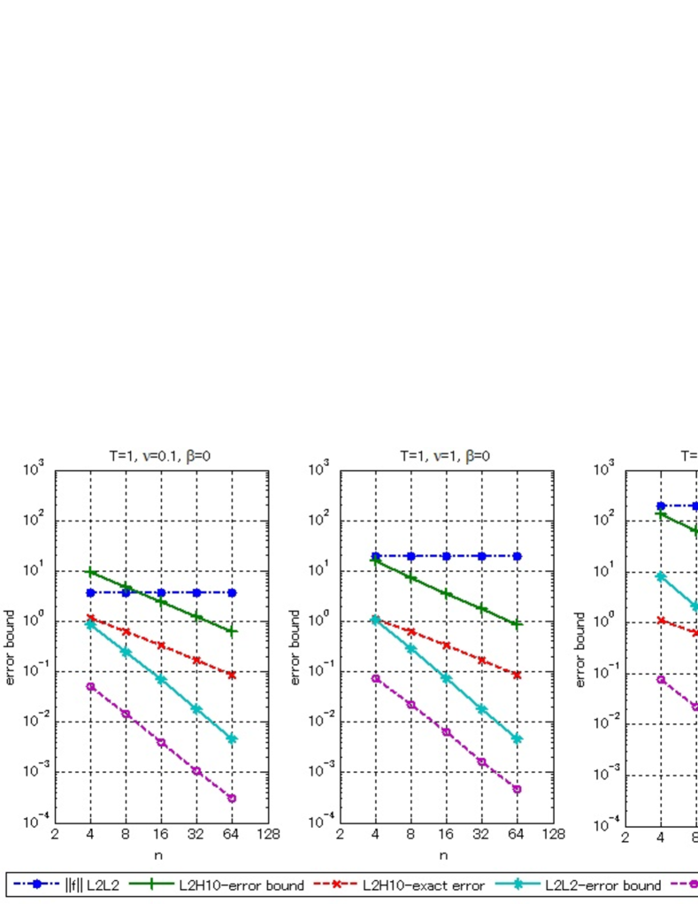
Figure 1:  L2H10 and L2L2 error estimates, $m=n^{2}$,  $\beta=0$,  $T=1$,  $\nu=0.1,~{}1,~{}10$,

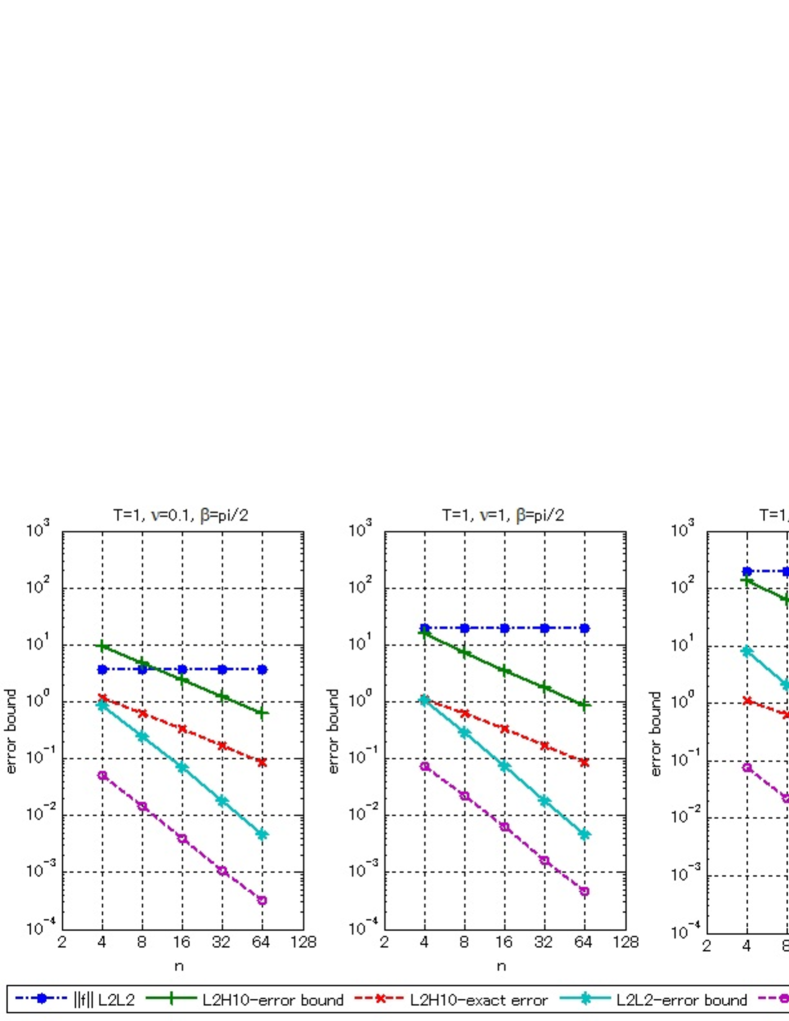
Figure 2:  L2H10 and L2L2 error estimates, $m=n^{2}$,  $\beta=0.5\pi$,  $T=1$,  $\nu=0.1,~{}1,~{}10$,

References

- [1] V. Barbu, Partial differential equations and boundary value problems, Kluwer Academic Publishers, the Netherland, 1998.
- [2] C. Bernardi, Numerical approximation of a periodic linear parabolic problem, SIAM Journal on Numerial Analysis, 19 (1982), 1196-1207.
- [3] J.-L. Figueras, M. Gameiro, J.-P. Lessard and R. de la Llave. A framework for the numerical computation and a posteriori verification of invariant objects of evolution equations. SIAM Journal on Applied Dynamical Systems 16(2), 1070-1088, 2017.
- [4] A. Hansbo, Error estimates for the numerical solution of a time-periodic linear parabolic problem, BIT 31, 664-685, 1991.
- [5] M.T. Nakao, T. Kinoshita and T. Kimura: On a posteriori estimates of inverse operators for linear parabolic initial-boundary value problems, Computing, 94, 151-162, 2012.
- [6] M.T. Nakao, K. Hashimoto, Y. Watanabe: A numerical method to verify the invertibility of linear elliptic operators with applications to nonlinear problems, Computing , 75, 1–14, 2005.
- [7] M. T. Nakao, T. Kimura, T. Kinoshita, Constructive a priori error estimates for a full discrete approximation of the heat equation, SIAM Journal on Numerial Analysis, 51 (2013), 1525-1541.
- [8] A.Pazy, Semigroups of Linear Operators and Applications to Partial Differential Equations, Springer, New York, 1983.
- [9] S.M. Rump, INTLAB - INTerval LABoratory. In Tibor Csendes, editor, Developments in Reliable Computing, pages 77-104. Kluwer Academic Publishers, Dordrecht, 1999.
- [10] M.H. Schultz, Spline Analysis, Prentice-Hall, N.J., 1973.
- [11] E. Zeidler, Nonlinear functional analysis and its applications II/B, Springer-Verlag, New York, 1990.
- [12] P. Zgliczynski, Rigorous Numerics for Dissipative PDEs III. An effective algorithm for rigorous integration of dissipative PDEs, Topological Methods in Nonlinear Analysis, 36 (2010), pp. 197–262