Information entropy and complexity measure in generalized Kratzer potential

Abstract

Shannon entropy ($S$), Fisher information ($I$) and a measure equivalent to Fisher-Shannon complexity $(C_{IS})$ of a ro-vibrational state of diatomic molecules (O₂, O${}_{2}^{+}$, NO, NO⁺) with generalized Kratzer potential is analyzed. Exact analytical expression of $I_{\mathrm{\mathbf{r}}}$ is derived for the arbitrary state, whereas the same could be done for $I_{\mathrm{\mathbf{p}}}$ with $\{n,\ell,m=0\}$ state. It is found that shifting from neutral to the cationic system, $I_{\mathrm{\mathbf{r}}}$ increases while $S_{\mathrm{\mathbf{r}}}$ decreases, consistent with the interpretation of a localization in the probability distribution. Additionally, this study reveals that $C_{IS}$ increases with the number of nodes in a system.

Keywords: diatomic molecule, generalized Kratzer potential, Fisher information, Shannon entropy, Fisher-Shannon complexity.

I Introduction

Ever since the early days of quantum mechanics, diatomic molecular potentials have received much attention due to their importance to describe intra-molecular and intermolecular interactions as well as atomic-pair correlations. Over the years, a large number of such potentials have been adopted in a multitude of physical/chemical problems. Since the literature is quite vast, here we mention a few prominent ones, such as generalized Morse, Mie, Kratzer-Fues, pseudoharmonic, non-central, deformed Rosen-Morse, generalized Woods-Saxon, Pöschl-Teller potential etc akcay12 . They have fundamental relevance and utility in quantum description of natural phenomena, processes and systems, not only in the 3D world, but also in non-relativistic and relativistic D-dimensional physics. This work focuses on generalized Kratzer (Kratzer-type) potential, which is a simple realistic zero-order model for describing the vibration-rotation motion of diatomic molecules. It has important properties like (i) correct asymptotic behaviour at $r=0$ and $r=\infty$ (ii) exactly solvable for a given state with an arbitrary angular momentum (iii) allows the system to dissociate, which is forbidden for a harmonic oscillator-based model. The mixed energy spectrum of this potential contains both discrete and continuum parts, corresponding to bound and scattering states respectively. While bound-state wave functions have been widely used in studies related to molecular spectroscopy, latter states are important in the context of the photo-dissociation process, diatomic molecular scattering, radiative recombination in an atom-atom collision adelio02 , etc. Recently its use as a universal potential for diatomic molecules has been reported in two excellent review articles hooydonk99 ; hooydonk00 . Apart from these, this has also been heavily studied in molecular, chemical and solid-state physics, due to its general feature of true interaction energy as well as interatomic, inter-molecular and dynamical properties kratzer20 ; fues26 ; oyewumi10 .

In recent years, there has been a burgeoning activity in studies related to information-theoretic measures in quantum chemical systems. The delocalizing properties of electronic distribution that characterize the quantum states of these molecular potentials have been analyzed quite extensively by information theoretical tools such as Shannon entropy ($S$) birula75 , Fisher information ($I$) romera05 , Rényi entropy ($R$) sen12 , Tsallis entropy ($T$) tsallis88 and Onicescu information energy ($E$) sen12 , in both position ($r$) and momentum ($p$) spaces. Amongst these $S$ and $I$ describe a system in a complementary way. The former is a global measure of the distribution of density. It is closely connected to the concept of entropy and disorder in thermodynamics. High values of $S_{\mathrm{\mathbf{r}}}$ are associated with low values of $S_{\mathrm{\mathbf{p}}}$ indicating a highly delocalized single-particle density distribution in $r$ space, and a localized one in $p$ space. It has a close relationship with quantities like kinetic energy, magnetic susceptibility and also has applications in the study of the dynamics of atoms and molecules. The total Shannon entropy ($S_{t}$), a sum of its $r$- and $p$-space counterparts, obeys the familiar entropic uncertainty relation: $S_{\mathrm{\mathbf{r}}}+S_{\mathrm{\mathbf{p}}}\geq d(1+\mathrm{ln}{\pi}$), where $d$ is associated dimension of the system. This is a stronger version of Heisenberg uncertainty relation as it incorporates higher order moments in it birula75 . On the other hand, $I$ is a cornerstone which signifies local inhomogeneity of single-particle density $\rho(\mathrm{\mathbf{r}})$ of a system under consideration. It is well-known that $I$ escalates with localization as well as fluctuation in probability density and diminishes in case of well spread-out densities. Of late, a spontaneity has been observed in the application of this information tool in various fields of physics and chemistry, mainly due to the fact that, the translationally invariant $I$ may be used as a quantitative measure of the spatial distribution of single-particle probability density of a many-particle system. It resembles the familiar Weiszäcker kinetic energy functional in density functional theory of electronic systems chakraborty12 . Numerous fundamental equations of physics and some conservation laws have also been derived using the property of $I$ as a basic variable of extreme physical information frieden04 ; nagy03 . Because of its versatile nature, it has potential application in exploring other different phenomena such as Pauli effect nagy06a ; toranzo14 , polarizability, ionization potential, steric effect nagy07 ; esquivel11 , elementary chemical reaction rosa10 , bond formation nalewajski08 , etc.

Statistical complexity ($C_{LMC}$) lopezruiz95 , another relevant concept, which arises due to breakdown of symmetry, is explicitly related to the aforementioned fundamental information theoretical tools. It represents a combined effect of two complementary quantities, offering a qualitative idea of the organization, structure and correlation in a system. It has finite value in a state lying between two limiting cases of complete order (maximum distance from equilibrium) and maximum disorder (at equilibrium). The statistical measure of complexity is nothing but the product of the information content $(H)$ and concentration of spatial distribution $(D)$, and can be written as $C_{LMC}=H.D$, which was later criticized catalan02 and modified sanchez05 to the form of $C_{LMC}=D.e^{S}$ ($S$ quantifies the information of the system) in order to satisfy few conditions; such as reaching minimal values for both extremely ordered and disordered limits, invariance under scaling, translation and replication. Various definitions were put forth in literature. Some notable ones include Shiner, Davidson and Landsberg (SDL) landsberg98 ; shiner99 , Fisher-Shannon ($C_{IS}$) romera04 ; sen07 ; angulo08 , Cramér-Rao dehesa06a ; angulo08 ; antolin09 , generalized Rényi-like calbet01 ; martin06 ; romera08 complexity, etc. Amongst these, $C_{IS}$ corresponds to a measure which probes a system in terms of complementary global and local factors, and also satisfies certain desirable properties in complexity, such as, invariance under translations and re-scaling transformations, invariance under replication, near-continuity, etc.sen12 . This has remarkable applications in the study of the atomic shell structure, ionization processes sen07 ; angulo08 ; antolin09 ; angulo08a , as well as in molecular properties like energy, ionization potential, hardness and dipole moment in the localization-delocalization plane showing chemically significant pattern esquivel10 , molecular reactivity studies welearegay14 . Few elementary chemical reactions such as hydrogenic-abstraction reaction esquivel11a , identity S${}_{N}^{2}$ exchange reaction molina-espiritu12 , and also concurrent phenomena occurring at the transition region esquivel12 of these reactions have been investigated through composite information-theoretic measures in conjugate spaces.

During the last few years, there has been a growing interest in studies on information theoretic and complexity measures in various model and real quantum systems. It is worthwhile mentioning a few selected works, viz., Morse dehesa06 , modified Yukawa and Hulthén patil07 , Dirac-delta bouvrie11 , Teitz-Wei diatomic molecular model falaye14 , squared tangent well dong14 , ring-shaped modified Kratzer yahya14 , symmetric trigonometric Rosen-Morse nath14 , pseudoharmonic yahya15 , hyperbolic double well sun15 , infinite circular well song15 , ring-shaped Mie yahya14 ; falaye15 , Pösch-Teller yahya16 ; dehesa06 , harmonic oscillator, generalized Morse onate16 , Eckart pooja16 , Frost-Muslin idiodi16 , Killingbeck, Eckart Manning Rosen, confined hydrogen atom majumdar17 ; mukherjee18 ; mukherjee18a etc. It may be noted that, a vast amount of elegant works have been published on eigenfunctions, eigenvalues and other properties of Schrödinger equation with these potentials, employing a variety of analytical/numerical methods, differing in their range of sophistication and accuracy. However, their information theoretical investigation is a rather recent development. Moreover, whilst most of these works on $I$ were carried out numerically, analytical works have been rather limited. In romera05 , the authors derived expressions for Fisher information in $r$ $(I_{\mathrm{\mathbf{r}}})$, and $p$ $(I_{\mathrm{\mathbf{p}}})$ spaces for an arbitrary quantum state of a single particle in a central potential in terms of radial expectation values $\{\langle p^{2}\rangle,\langle r^{-2}\rangle\}$ and $\{\langle r^{2}\rangle,\langle p^{-2}\rangle\}$.

While several papers have reported the energy spectrum (variety of approximate theoretical methods, as well as exact solution) of this potential, our present work focuses on the probability distribution through information measures such as $I,S,C_{IS}$, in both $r,p$ spaces in an arbitrary state, characterized by quantum numbers $n,\ell,m$ respectively. Starting from exact $r$-space wave functions (as reported in oyewumi10 , through a factorization method), we first derive closed-form analytical expressions for $I_{\mathrm{\mathbf{r}}}$ for any given $n,\ell,m$. It has been possible to obtain similar expressions for $I_{\mathrm{\mathbf{p}}}$ as well, but only when $m=0$. The $p$-space wave function is numerically obtained from the Fourier transform of the $r$-space counterpart. Simplified analytical formulas are derived also for $S_{\mathrm{\mathbf{r}}}$; in this case, however, closed-form expressions are not possible; rather these are written in terms of some entropy integrals involving classical orthogonal polynomials. Accurate results are presented for $I_{\mathrm{\mathbf{r}}},I_{\mathrm{\mathbf{p}}},S_{\mathrm{\mathbf{r}}},S_{\mathrm{\mathbf{p}}}$ as well as $C_{IS}$, for representative states, in four selected diatomic molecules (two homo-nuclear, two hetero-nuclear) including two cations, namely O₂, O${}_{2}^{+}$, NO, NO⁺. Results are carefully monitored in both ground and excited states. Also, the system-dependence of scaling parameter $b$ in complexity measure is discussed. The article is organized as follows: Sec. II gives a brief description of the theoretical method to find probability distribution and the desired information measures in a particular state. Then Sec. III offers a thorough discussion of the results; finally, a few concluding remarks are stated in Sec. IV.

II Methodology

The generalized Kratzer potential oyewumi10 may be represented in the following form,

$$v(r)=\frac{x}{r}+\frac{y}{r^{2}}+z.$$ (1)

This is usually recast in following two alternative equivalent ways:

1. Kratzer-Fues potential, given by,

   $$v(r)=-D_{0}\left(\frac{2r_{0}}{r}-\frac{{r_{0}}^{2}}{r^{2}}\right),\ \ \ \ \mathrm{with}\ \ x=-2D_{0}r_{0},\ y=D_{0}{r_{0}}^{2},\ z=0,$$ (2)

   where $D_{0}$ and $r_{0}$ represent the dissociation energy between two atoms and equilibrium intermolecular separation respectively.

2. Modified Kratzer or Mie potential, expressed as,

   $$v(r)=-D_{0}\left(\frac{2r_{0}}{r}-\frac{{r_{0}}^{2}}{r^{2}}\right)+D_{0}=D_{0}\left(\frac{r-r_{0}}{r}\right)^{2},\mathrm{with}\ \ x=-2D_{0}r_{0},\ y=D_{0}{r_{0}}^{2},\ z=D_{0}.$$ (3)

Without any loss of generality, the time-independent non-relativistic wave function for a single particle in co-ordinate space can be written as ($\mathrm{\mathbf{r}}=\{r,\Omega\}$),

$$\Psi_{n,\ell,m}(\mathrm{\mathbf{r}})=\psi_{n,\ell}(r)\ Y_{\ell,m}(\Omega),$$ (4)

with $r$ and $\Omega$ denoting radial distance and solid angle respectively. Here $\psi_{n,\ell}(r)$ corresponds to the radial part and $Y_{\ell,m}(\Omega)$ the spherical harmonics of atomic state, determined by quantum numbers $(n,\ell,m)$. In what follows, atomic unit is employed unless otherwise mentioned and $\mathrm{\mathbf{r}},\mathrm{\mathbf{p}}$ subscripts denote quantities in full $r$ and $p$ spaces (including angular part) respectively.

Adopting the potential in Eq. (3), the relevant radial Schrödinger equation of the motion of a particle with reduced mass $\mu$ in a spherically symmetric potential $v(r)$ becomes,

$$\left[-\frac{1}{2\mu}\ \frac{d^{2}}{dr^{2}}+\frac{\ell(\ell+1)}{2r^{2}}+v(r)\right]\psi_{n,\ell}(r)={E}_{n,\ell}\ \psi_{n,\ell}(r).$$ (5)

Note that, throughout the present work, we shall deal with this form of potential, as Eq. (2) constitutes a special case of it. The angular part has following common form in $r,p$ spaces,

$$Y_{\ell,m}({\Omega})=\Theta_{\ell,m}(\theta)\ \Phi_{m}(\phi)=(-1)^{m}\sqrt{\frac{2l+1}{4\pi}\frac{(\ell-m)!}{(\ell+m)!}}\ P_{\ell}^{m}(\cos\theta)\ e^{-im\phi},$$ (6)

with $P_{\ell}^{m}(\cos\theta)$ signifying the usual associated Legendre polynomial. The exact normalized radial wave function for this potential has been obtained with the factorization method oyewumi10 ,

$$\psi_{n,\ell}(r)=N_{n,\ell}\ e^{-\frac{\xi r}{2}}r^{\beta_{\ell}}\ L^{2{\beta_{\ell}}+1}_{n}\left(\xi r\right)$$ (7)

where $L^{2{\beta_{\ell}}+1}_{n}\left(\xi r\right)$ is denoted the Associated Laguerre polynomial and the normalization constant has form,

$$N_{n,\ell}=\left[\frac{\xi^{2\beta_{\ell}+3}}{2}\frac{n!}{\left(n+\beta_{\ell}+1\right)\Gamma\left(n+2\beta_{\ell}+2\right)}\right]^{\frac{1}{2}}.$$ (8)

Here, the quantities $\xi$ and $\beta_{\ell}$ are defined as below,

$$\xi={\left[-8\mu\left({E}_{n,\ell}-z\right)\right]}^{\frac{1}{2}},\ \ \ \ \ \ \beta_{\ell}=\frac{1}{2}\left[-1+\sqrt{(2\ell+1)^{2}+8\mu y}\right].$$ (9)

The corresponding bound-state eigenvalues are written as,

$$E_{n,\ell}=\frac{-\mu x^{2}}{2\left[n+\beta_{\ell}+1\right]^{2}}+z.$$ (10)

The wave function in p space is obtained by taking usual Fourier transformation of the r-space counterpart and as such given by the standard expression,

$$\Xi_{n,\ell}(p) = \frac{1}{(2\pi)^{\frac{3}{2}}}\ \int_{0}^{\infty}\int_{0}^{\pi}\int_{0}^{2\pi}\psi_{n,\ell}(r)\ \Theta(\theta)\Phi(\phi)\ e^{ipr\cos\theta}r^{2}\sin\theta\ \mathrm{d}r\mathrm{d}\theta\mathrm{d}\phi,$$ (11)

where $\Xi_{n,\ell}(p)$ needs to be normalized. Integrations over $\theta$ and $\phi$ have been done analytically. Depending on $\ell$ the coefficients of integration vary; these have been discussed and tabulated in mukherjee18a . Thus the normalized $r$- and $p$-space electron densities can be expressed as, $\rho(\mathrm{\mathbf{r}})=|\Psi_{n,\ell,m}(\mathrm{\mathbf{r}})|^{2}=|\psi_{n,\ell}(r)|^{2}\ |Y_{\ell,m}(\Omega)|^{2}$ and $\Pi(\mathrm{\mathbf{p}})=|\Lambda_{n,\ell,m}(\mathrm{\mathbf{p}})|^{2}=|\Xi_{n,\ell}(p)|^{2}\ |Y_{\ell,m}(\Omega)|^{2}$ respectively.

Now, following romera05 , Fisher information of a single particle in a central potential can be simplified in terms of radial expectation values in $r$ and $p$ spaces, as below romera05 ,

$$I_{\mathrm{\mathbf{r}}} =\int_{{\mathcal{R}}^{3}}\left[\frac{|\nabla\rho(\mathrm{\mathbf{r}})|^{2}}{\rho(\mathrm{\mathbf{r}})}\right]\mathrm{d}\mathrm{\mathbf{r}}=4\langle p^{2}\rangle-2(2\ell+1)|m|\langle r^{-2}\rangle$$ (12)

$$I_{\mathrm{\mathbf{p}}} =\int_{{\mathcal{R}}^{3}}\left[\frac{|\nabla\Pi(\mathrm{\mathbf{p}})|^{2}}{\Pi(\mathrm{\mathbf{p}})}\right]\mathrm{d}\mathrm{\mathbf{p}}=4\langle r^{2}\rangle-2(2\ell+1)|m|\langle p^{-2}\rangle.$$

When $m=0$, $I_{\mathrm{\mathbf{r}}}$ and $I_{\mathrm{\mathbf{p}}}$ assume simpler expressions,

$$I_{\mathrm{\mathbf{r}}}=4\langle p^{2}\rangle,\hskip 8.53581pt\ \ \ \ I_{\mathrm{\mathbf{p}}}=4\langle r^{2}\rangle.$$ (13)

It has been established that the general Heisenberg-like uncertainty relation associated with a particle in a $D$-dimensional central potential can be expressed as moreno06 ,

$$\left\langle r^{2}\right\rangle\left\langle p^{2}\right\rangle\ \geqslant\left(L+\frac{3}{2}\right)^{2},$$ (14)

where $L=\ell+\frac{D-3}{2}$ is generalized angular momentum (grand orbital quantum number). From this modified Heisenberg relation, $I$-based uncertainty relation transforms into dehesa07 ,

$$I_{\mathrm{\mathbf{r}}}I_{\mathrm{\mathbf{p}}}\geqslant 16\left(1-\frac{2|m|}{2L+1}\right)^{2}\left(L+\frac{3}{2}\right)^{2}.$$ (15)

For the particular case of $D=3$, Eqs. (14) and (15) lead to following bounds,

$$\left\langle r^{2}\right\rangle\left\langle p^{2}\right\rangle \geqslant\left(\ell+\frac{3}{2}\right)^{2}$$ (16)

$$I_{\mathrm{\mathbf{r}}}I_{\mathrm{\mathbf{p}}} \geqslant 16\left(1-\frac{2|m|}{2l+1}\right)^{2}\left(\ell+\frac{3}{2}\right)^{2}.$$

Table 1: Spectroscopic parameters of diatomic molecules studied in this work, taken from falaye14 .

Molecule (state)	$\mu/10^{-23}$ (g)	$D_{0}$ (cm${}^{-1})$	$r_{0}$ (Å)
O2 $(X^{3}\Sigma_{g}^{+})$	1.337	42041	1.207
O${}_{2}^{+}$ $(X^{2}\Pi_{g})$	1.337	54688	1.116
NO $(X^{2}\Sigma_{r})$	1.249	53341	1.151
NO+ $(X^{1}\Sigma^{+})$	1.239	88694	1.063

Next, $S$ in conjugate $r$ and $p$ spaces (in spherical polar coordinates) can be written as,

$$\begin{aligned} S_{\mathrm{\mathbf{r}}}=-\int_{{\mathcal{R}}^{3}}\rho(\mathrm{\mathbf{r}})\ \ln[\rho(\mathrm{\mathbf{r}})]\ \mathrm{d}\mathrm{\mathbf{r}}=2\pi\left(S_{r}+S_{(\theta,\phi)}\right),\\ S_{\mathrm{\mathbf{p}}}=-\int_{{\mathcal{R}}^{3}}\Pi(\mathrm{\mathbf{p}})\ \ln[\Pi(\mathrm{\mathbf{p}})]\ \mathrm{d}\mathrm{\mathbf{p}}=2\pi\left(S_{p}+S_{(\theta,\phi)}\right),\\ {\color[rgb]{1,0,0}S_{\mathrm{\mathbf{r}}}+S_{\mathrm{\mathbf{p}}}=S_{t}\geq d(1+\ln\pi),}\end{aligned}$$ (17)

where d is the dimension of the system.
The quantities $S_{r},S_{p}$ and $S_{\theta}$ have been defined as birula75 ,

$$\begin{aligned} S_{r}&=-\int_{0}^{\infty}\rho(r)\ \ln[\rho(r)]r^{2}\mathrm{d}r,\ \hskip 71.13188pt\rho(r)=|\psi_{n,\ell}(r)|^{2},\\ S_{p}&=-\int_{0}^{\infty}\Pi(p)\ln[\Pi(p)]\ p^{2}\mathrm{d}p,\hskip 62.59605pt{\color[rgb]{1,0,0}\Pi(p)=|\Xi_{n,\ell}(p)|^{2},}\\ S_{(\theta,\phi)}&=-\int_{0}^{\pi}\chi(\theta)\ \ln[\chi(\theta)]\sin\theta\mathrm{d}\theta,\hskip 56.9055pt\chi(\theta)=|\Theta(\theta)|^{2}.\end{aligned}$$ (18)

Finally, the Fisher-Shannon complexity is defined as ($b$ is a scaling factor) romera04 ,

$$C_{IS}=Ie^{bS}.$$ (19)

III Result and Discussion

At first, it may be prudent to mention a few things to facilitate the forthcoming discussion. As hinted before, apart from $I_{\mathrm{\mathbf{r}}}$ (all states) and $I_{\mathrm{\mathbf{p}}}$ (only $m=0$), all other quantities like $I_{\mathrm{\mathbf{p}}}$ ($m\neq 0$), as well as $S_{\mathrm{\mathbf{r}}}$, $S_{\mathrm{\mathbf{p}}}$ and $C_{IS}$, presented in this work are calculated numerically. All the tables and figures contain the net information measures in conjugate $r$ and $p$ spaces, which can be separated into radial and angular components. It is evident from Eq. (12) that in both $I_{\mathrm{\mathbf{r}}}$ and $I_{\mathrm{\mathbf{p}}}$ expressions, angular parts are normalized to unity; thus evaluation of these quantities using only radial parts will suffice the purpose. The complexity measures of Eq. (19) have been probed for two selected values of $b$, viz., 1 and $\frac{2}{3}$, which are the most often used values in literature. Amongst these, the latter is usually referred as $C_{IS}$. A simplified notation, $C_{I_{s},S_{s}}^{b}$ is used throughout our discussion for convenience, where the subscripts “s” is used to specify the conjugate space r or p. The superscript “b” takes two values identifying two scaling parameters $\frac{2}{3}$ and $1$. All results are presented here for four representative diatomic molecules, namely, O₂, O${}_{2}^{+}$, NO, NO⁺, which have the model parameters listed in Table I; these are adopted from reference falaye14 . It is worthwhile mentioning that, convergence of all numerically calculated quantities were carefully checked with respect to the grid parameters and some of these have been detailed earlier mukherjee18 in the context of a confined H atom embedded inside an impenetrable spherical cavity; hence not repeated here. These are checked for convergence up to the place they are given. Lastly, since the exact solution including energy spectrum as well as eigenfunctions have already been reported by a number of authors in literature, we do not discuss these here any more.

Table 2: $I_{\mathrm{\mathbf{r}}}^{\updownarrow\updownarrow},~{}I_{\mathrm{\mathbf{p}}}^{\dagger\dagger}$ and $I_{t}$ for some selected states of four diatomic molecules. See text for details.

	O2			O${}_{2}^{+}$			NO			NO+
$n^{\updownarrow}$	$I_{\mathrm{\mathbf{r}}}$	$I_{\mathrm{\mathbf{p}}}$	$I_{t}$	$I_{\mathrm{\mathbf{r}}}$	$I_{\mathrm{\mathbf{p}}}$	$I_{t}$	$I_{\mathrm{\mathbf{r}}}$	$I_{\mathrm{\mathbf{p}}}$	$I_{t}$	$I_{\mathrm{\mathbf{r}}}$	$I_{\mathrm{\mathbf{p}}}$	$I_{t}$	$I_{t}^{\P}$
0	65.367653	21.239249	1388.35	80.657917	18.138248	1462.99	74.644253	19.299666	1440.60	104.053919	16.410317	1707.55	36
1	192.338431	22.110305	4252.66	237.565501	18.843575	4476.58	219.790637	20.062002	4409.44	307.288984	16.955810	5210.33	36
2	314.931505	23.000945	7243.72	389.338510	19.563941	7616.99	360.113455	20.840849	7505.07	504.823940	17.511254	8840.10	36
3	433.296652	23.911420	10360.73	536.143741	20.299530	10883.46	495.772076	21.636412	10726.72	696.817662	18.076752	12596.20	36
4	547.577993	24.841985	13602.92	678.142011	21.050528	14275.24	626.919800	22.448896	14073.65	883.424127	18.652408	16477.48	36
5	657.914225	25.792896	16969.51	815.488386	21.817121	17791.60	753.704368	23.278510	17545.11	1064.792586	19.238329	20484.83	36
$\ell^{\dagger}$
0	657.914225	25.792896	16969.51	815.488386	21.817121	17791.60	753.704368	23.27851	17545.11	1064.792586	19.238329	20484.83	36
1	659.247075	25.796242	17006.09	817.058906	21.819672	17827.95	755.17771	23.281317	17581.53	1066.557661	19.239985	20520.55	100
2	661.911687	25.802935	17079.26	820.198793	21.824776	17900.65	758.123278	23.286931	17654.36	1070.086862	19.243298	20592.00	196
3	665.905888	25.812976	17189.01	824.905745	21.832433	18009.69	762.538843	23.295354	17763.61	1075.378295	19.248269	20699.17	324
4	671.226423	25.826367	17335.33	831.176311	21.842644	18155.08	768.421066	23.306587	17909.27	1082.429122	19.254896	20842.06	484
5	677.868959	25.843111	17518.24	839.005895	21.855411	18336.81	775.7655	23.320632	18091.34	1091.235561	19.263183	21020.67	676
$m^{\ddagger}$
0	677.868959	25.843111	17518.24	839.005895	21.855411	18336.81	775.765500	23.320632	18091.34	1091.235561	19.263183	21020.67	676
1	674.031036	25.249005	17018.61	834.493874	21.369094	17832.37	771.529881	22.7966953	17588.33	1086.195415	18.8743977	20501.28	$\frac{54756}{121}$
2	670.193113	24.654900	16523.54	829.981852	20.882778	17332.32	767.294262	22.2727585	17089.75	1081.155269	18.4856120	19985.81	$\frac{33124}{121}$
3	666.355189	24.060795	16033.03	825.469831	20.396461	16836.66	763.058644	21.7488218	16595.62	1076.115123	18.096826	19474.26	$\frac{16900}{121}$
4	662.517266	23.466689	15547.08	820.957809	19.910144	16345.38	758.823025	21.2248850	16105.93	1071.074976	17.708040	18966.63	$\frac{6084}{121}$
5	658.679343	22.872584	15065.69	816.445788	19.423827	15858.50	754.587406	20.7009483	15620.67	1066.03483	17.31925	18462.92	$\frac{676}{121}$

${}^{\updownarrow}\ell$ and $m$ are fixed at $0$.          ${}^{\dagger}n$ and $m$ are fixed at $5$ and $0$ respectively.          ${}^{\ddagger}n$ and $\ell$ both are fixed at $5$.          ↕↕Calculated from Eq. (27).

††In a state having $m=0$, these are calculated from Eq. (28). For all other states, these are obtained numerically.

¶Lower bounds of $I_{t}=I_{\mathrm{\mathbf{r}}}I_{\mathrm{\mathbf{p}}}$, obtained from Eq. (16). In all cases, the products satisfy this bound.

Now let us proceed for evaluation of $I_{\mathrm{\mathbf{r}}}$ and $I_{\mathrm{\mathbf{p}}}$, for which some expectation values are needed. This can be achieved by means of the following sequence of steps; first is to write the Hamiltonian in following convenient form,

$$H=\frac{p^{2}}{2\mu}+\left[-D_{0}\left(\frac{2r_{0}}{r}-\frac{{r_{0}}^{2}}{r^{2}}\right)+z\right].$$ (20)

This prompts us to write $\left\langle p^{2}\right\rangle$ as,

$$\langle p^{2}\rangle=2\mu\langle H\rangle-2\mu z+4\mu D_{0}r_{0}\left\langle\frac{1}{r}\right\rangle-2\mu D_{0}r_{0}^{2}\left\langle\frac{1}{r^{2}}\right\rangle,$$ (21)

from which it is apparent that, in order to evaluate $\left\langle p^{2}\right\rangle$, one is required to compute the additional expectation values such as: $\left\langle H\right\rangle$, $\left\langle\frac{1}{r}\right\rangle$ and $\left\langle\frac{1}{r^{2}}\right\rangle$. The first term $\left\langle H\right\rangle$ is nothing but the energy eigenvalue of a particular state with definite values of $n,\ell$, and can be easily calculated from Eq. (10). Next, we turn to $\left\langle\frac{1}{r}\right\rangle$, which can be carried out as below,

$$\left\langle\frac{1}{r}\right\rangle=\int_{0}^{\infty}|N_{n,\ell}|^{2}e^{{\xi}r}r^{2\beta_{\ell}+1}\left[L^{2{\beta_{\ell}}+1}_{n}(r)\right]^{2}\mathrm{d}r=|N_{n,\ell}|^{2}\left(\frac{1}{\xi}\right)^{\left(2\beta_{\ell}+2\right)}\frac{\left(n+2\beta_{\ell}+1\right)!}{n!},$$ (22)

where we have used the standard integral form of Associated Laguerre polynomial gradshteyn07 ,

$$\int_{0}^{\infty}t^{\alpha}e^{-t}\left[L^{\alpha}_{n}(t)\right]^{2}\mathrm{d}t=\frac{(n+\alpha)!}{n!}.$$ (23)

Also, $\left\langle\frac{1}{r^{2}}\right\rangle$ can be calculated as,

$$\left\langle\frac{1}{r^{2}}\right\rangle =\int_{0}^{\infty}|N_{n,\ell}|^{2}e^{{\xi}r}r^{2\beta_{\ell}}\left[L^{2{\beta_{\ell}}+1}_{n}(r)\right]^{2}\mathrm{d}r$$ (24)

$$=|N_{n,\ell}|^{2}\left(\frac{1}{\xi}\right)^{\left(2\beta_{\ell}+1\right)}\sum_{i=0}^{n}\left(\begin{array}[]{c}-1\\ n-i\end{array}\right)^{2}\frac{\Gamma\left(2\beta_{\ell}+1+i\right)}{i!}$$

which makes use of the following standard integral gradshteyn07 ,

$$\int_{0}^{\infty}t^{\alpha+\beta}e^{-t}\left[L^{\alpha}_{n}(t)\right]^{2}\mathrm{d}t=\sum_{i=0}^{n}\left(\begin{array}[]{c}\beta\\ n-i\end{array}\right)^{2}\frac{\Gamma\left(\alpha+\beta+1+i\right)}{i!}.$$ (25)

Finally, $\left\langle r^{2}\right\rangle$ reads,

$$\left\langle{r^{2}}\right\rangle =\int_{0}^{\infty}|N_{n,\ell}|^{2}e^{{\xi}r}r^{2\beta_{\ell}+4}\left[L^{2{\beta_{\ell}}+1}_{n}(r)\right]^{2}\mathrm{d}r$$ (26)

$$=|N_{n,\ell}|^{2}\left(\frac{1}{\xi}\right)^{\left(2\beta_{\ell}+5\right)}\sum_{i=0}^{n}\left(\begin{array}[]{c}3\\ n-i\end{array}\right)^{2}\frac{\Gamma\left(2\beta_{\ell}+5+i\right)}{i!},$$

where once again the standard integral form given in Eq. (25) has been utilized.

Next the substitution of radial expectations values $\left\langle p^{2}\right\rangle$ and $\left\langle r^{-2}\right\rangle$, of Eqs. (21) and (24) in Eq. (12) yields the desired expression of $I_{\mathrm{\mathbf{r}}}$ in a particular state,

$$I_{\mathrm{\mathbf{r}}} =4\left[2\mu\left\langle H\right\rangle-2\mu z+4\mu D_{0}r_{0}\left\langle\frac{1}{r}\right\rangle-2\mu D_{0}{r_{0}}^{2}\left\langle\frac{1}{r^{2}}\right\rangle\right]-2(2\ell+1)|m|\left\langle\frac{1}{r^{2}}\right\rangle$$ (27)

$$=8\mu E_{n,\ell}-8\mu z+16\mu D_{0}r_{0}\left[|N_{n,\ell}|^{2}\left(\frac{1}{\xi}\right)^{\left(2\beta_{\ell}+2\right)}\frac{\left(n+2\beta_{\ell}+1\right)!}{n!}\right]-$$

$$\left\{8\mu D_{0}{r_{0}}^{2}-2(2\ell+1)|m|\right\}\left[|N_{n,\ell}|^{2}\left(\frac{1}{\xi}\right)^{\left(2\beta_{\ell}+1\right)}\sum_{i=0}^{n}\left(\begin{array}[]{c}-1\\ n-i\end{array}\right)^{2}\frac{\Gamma\left(2\beta_{\ell}+1+i\right)}{i!}\right].$$

Similarly, $I_{\mathrm{\mathbf{p}}}$ for $m=0$ states, can be simplified as,

$$I_{\mathrm{\mathbf{p}}}=4\left\langle r^{2}\right\rangle=4|N_{n,\ell}|^{2}\left(\frac{1}{\xi}\right)^{\left(2\beta_{\ell}+5\right)}\sum_{i=0}^{n}\left(\begin{array}[]{c}3\\ n-i\end{array}\right)^{2}\frac{\Gamma\left(2\beta_{\ell}+5+i\right)}{i!},$$ (28)

where the expression of $\langle r^{2}\rangle$ in Eq. (26) has been employed.

Now we are ready to present our estimated $I_{\mathrm{\mathbf{r}}}$ and $I_{\mathrm{\mathbf{p}}}$ values in Table II. Towards this goal, a cross-section of results are given for O₂, O${}_{2}^{+}$, NO and NO⁺. For each molecule, these dual measures in conjugate spaces are given in three horizontally separated regions; each one referring to the variation of one state index, keeping other two fixed. Thus the top, middle and bottom segments characterize states varying $n,\ell$ and $m$ respectively. State indices alter in the range of $0-5$. It is noticed that, in all these states, both $I_{\mathrm{\mathbf{r}}},I_{\mathrm{\mathbf{p}}}$ increase with an increase in $n$ for fixed $\ell,m$. This is to be expected, as, with rise in $n$, number of nodes grows, which promotes fluctuation. Equation (12) suggests that for $m=0$ states, $I_{\mathrm{\mathbf{r}}}$ may be associated with the kinetic energy of the system. Hence, as $n$ (at fixed $\ell,m$) advances, $I_{\mathrm{\mathbf{r}}}$ accumulates indicating a rise in kinetic energy. The table also reflects that, both $I_{\mathrm{\mathbf{r}}},I_{\mathrm{\mathbf{p}}}$ progress with $\ell$ (at fixed $n,m$). Note that, in this potential, the number of nodes in a given state depends only on $n$. Therefore, at some particular $n,m$ values, the rise in $I_{\mathrm{\mathbf{r}}}$ and $I_{\mathrm{\mathbf{p}}}$ with $\ell$ indicates the enhancement of fluctuation in states having a fixed number of nodes. However, they both decline with growth in $m$ (at fixed $n,\ell$). Furthermore, $I_{\mathrm{\mathbf{r}}}$ in cationic systems possess higher values than their neutral counterparts. In both O₂ and NO, on going from the neutral to cationic species, $D_{0}$ increases while $r_{0}$ decreases, indicating an increase in bond strength. This results in an enhancement of localization, which is reflected in the growth of $I_{\mathrm{\mathbf{r}}}$. In addition, from the reported values in this table, $I_{t}$ can easily be found to satisfy the lower bound given in Eq. (16) in terms of $I_{\mathrm{\mathbf{r}}}$ and $I_{\mathrm{\mathbf{p}}}$.

Table 3: $S_{\mathrm{\mathbf{r}}},~{}S_{\mathrm{\mathbf{p}}}$ and $S_{t}^{\P}$ for some selected states of four diatomic molecules. See text for details.

	O2			O${}_{2}^{+}$			NO			NO+
$n^{\updownarrow}$	$S_{\mathrm{\mathbf{r}}}$	$S_{\mathrm{\mathbf{p}}}$	$S_{t}$	$S_{\mathrm{\mathbf{r}}}$	$S_{\mathrm{\mathbf{p}}}$	$S_{t}$	$S_{\mathrm{\mathbf{r}}}$	$S_{\mathrm{\mathbf{p}}}$	$S_{t}$	$S_{\mathrm{\mathbf{r}}}$	$S_{\mathrm{\mathbf{p}}}$	$S_{t}$
0	3.5256409472	6.0023	9.5279	3.2629165502	6.3142	9.5771	3.3636640774	6.1989	9.5625	3.0359854245	6.6868	9.7227
1	3.831160	8.1101	11.9412	3.566630	8.4270	11.9936	3.667899	8.3103	11.9781	3.334892	8.8133	12.1481
2	4.021609	8.3220	12.3436	3.755314	8.6378	12.3931	3.857093	8.5214	12.3784	3.518875	9.0207	12.5395
3	4.166878	9.0066	13.1734	3.898848	9.3257	13.2245	4.001129	9.2084	13.2095	3.65778	9.7173	13.3750
4	4.287550	9.1319	13.4194	4.017814	9.4500	13.4678	4.120588	9.3330	13.4535	3.77219	9.8398	13.6119
5	4.392598	9.5278	13.9203	4.121181	9.8486	13.9697	4.224441	9.7308	13.9552	3.87107	10.2464	14.1174
$\ell^{\dagger}$
0	4.392598	9.5278	13.9203	4.121181	9.8486	13.9697	4.224441	9.7308	13.9552	3.87107	10.2464	14.1174
1	3.960834	9.109	13.0698	3.689399	9.4294	13.1187	3.792664	9.3117	13.1043	3.43924	9.8241	13.2633
2	3.903244	9.0711	12.9743	3.631773	9.3903	13.0220	3.735048	9.273	13.0080	3.38153	9.7835	13.1200
3	3.883322	9.0749	12.9582	3.611798	9.3934	13.0051	3.715089	9.2763	12.9913	3.36142	9.7832	13.1446
4	3.873926	9.0938	12.9677	3.602330	9.4105	13.0128	3.705641	9.2938	12.9994	3.35178	9.7965	13.1482
5	3.868874	9.1189	12.9877	3.597188	9.4348	13.0319	3.700524	9.3185	13.0190	3.34642	9.8174	13.1638
$m^{\ddagger}$
0	3.868874	9.1189	12.9877	3.597188	9.4348	13.0319	3.700524	9.3185	13.0190	3.34642	9.8174	13.1638
1	3.9858	9.2358	13.2216	3.714114	9.5517	13.2658	3.81745	9.4354	13.2528	3.46335	9.9344	13.3977
2	4.040809	9.2908	13.3316	3.769123	9.6067	13.3758	3.872459	9.4904	13.3628	3.51836	9.9894	13.5077
3	4.049226	9.2992	13.3484	3.77754	9.6152	13.3927	3.880876	9.4988	13.3796	3.52677	9.9978	13.5245
4	4.000479	9.2505	13.2509	3.728793	9.5664	13.2951	3.832129	9.4501	13.2822	3.47803	9.949	13.4270
5	3.833436	9.0834	12.9168	3.56175	9.3994	12.9611	3.665086	9.283	12.9480	3.31098	9.782	13.0929

${}^{\updownarrow}\ell$ and $m$ are fixed at $0$.                                             ${}^{\dagger}n$ and $m$ are fixed at $5$ and $0$ respectively.                                             ${}^{\ddagger}n$ and $\ell$ both are fixed at $5$.

¶Lower bounds of $S_{t}(=S_{\mathrm{\mathbf{r}}}+S_{\mathrm{\mathbf{p}}})$ is 6.43418 followed by the Eq. $S_{\mathrm{\mathbf{r}}}+S_{\mathrm{\mathbf{p}}}\geq d(1+\ln\pi)$.

Now we shift our focus on to $S$ in such a potential. First note that, single-particle probability density in an arbitrary state in $r$ space may be written as,

$$\rho(\mathrm{\mathbf{r}})={\left|N_{n,\ell}\right|}^{2}\ e^{-{\xi r}}r^{2{\beta_{\ell}}}\ {\left[L^{2{\beta_{\ell}}+1}_{n}\left(\xi r\right)\right]}^{2}\ {\left[Y_{\ell,m}\left({\Omega}\right)\right]}^{2}.$$ (29)

One can then decompose $S_{\mathrm{\mathbf{r}}}$ in terms of following five integrals,

$$S_{\mathrm{\mathbf{r}}}=-\int{\rho}\left({\mathrm{\mathbf{r}}}\right)\ln{\rho}\left({\mathrm{\mathbf{r}}}\right)\mathrm{d}\mathrm{\mathbf{r}}\\ =-(S_{1}+S_{2}+S_{3}+S_{4}+S_{5})$$ (30)

where,

$$S_{1} =\int{\rho}\left({\mathrm{\mathbf{r}}}\right)\ln{\left|N_{n,\ell}\right|}^{2}\mathrm{d}\mathrm{\mathbf{r}}=\ln{\left|N_{n,\ell}\right|}^{2},$$ (31)

$${\color[rgb]{1,0,0}S_{2}} ={\color[rgb]{1,0,0}-\int\xi r{\rho}\left({\mathrm{\mathbf{r}}}\right)\mathrm{d}\mathrm{\mathbf{r}}}\ \ ={\color[rgb]{1,0,0}-|N_{n,\ell}|^{2}\left(\frac{1}{\xi}\right)^{\left(2\beta_{\ell}+3\right)}\sum_{i=0}^{n}\left(\begin{array}[]{c}2\\ n-i\end{array}\right)^{2}\frac{\Gamma\left(2\beta_{\ell}+4+i\right)}{i!}},$$

$$S_{3}= 2\beta_{\ell}\int{\rho}\left({\mathrm{\mathbf{r}}}\right)\ln{r}\ \mathrm{d}\mathrm{\mathbf{r}}=-2\beta_{\ell}|N_{n,\ell}|^{2}\left(\frac{1}{\xi}\right)^{\left(2\beta_{\ell}+3\right)}\ (\ln{\xi})\sum_{i=0}^{n}\left(\begin{array}[]{c}1\\ n-i\end{array}\right)^{2}\frac{\Gamma\left(2\beta_{\ell}+3+i\right)}{i!}+\$$ (32)

$$2\beta_{\ell}|N_{n,\ell}|^{2}\left(\frac{1}{\xi}\right)^{\left(2\beta_{\ell}+3\right)}\int t^{\left(2\beta_{\ell}+2\right)}e^{-t}\left[L^{\left(2\beta_{\ell}+2\right)}_{n}(t)\right]^{2}\ln{t}\ \mathrm{d}t,$$

$$S_{4}= \int{\rho}\left({\mathrm{\mathbf{r}}}\right)\ln{\left[L^{\left(2\beta_{\ell}+1\right)}_{n}(\xi r)\right]^{2}}\mathrm{d}\mathrm{\mathbf{r}}$$

$$= |N_{n,\ell}|^{2}\left(\frac{1}{\xi}\right)^{\left(2\beta_{\ell}+3\right)}\int t^{\left(2\beta_{\ell}+2\right)}e^{-t}\left[L^{\left(2\beta_{\ell}+2\right)}_{n}(t)\right]^{2}\ln{\left[L^{\left(2\beta_{\ell}+2\right)}_{n}(t)\right]^{2}}\ \mathrm{d}t,$$

$$S_{5}=\int\left[Y_{\ell,m}\left({\Omega}\right)\right]^{2}\ln{\left[Y_{\ell,m}\left({\Omega}\right)\right]}^{2}\mathrm{d}{\Omega},$$ (33)

where we have defined $t={\xi}r$. Further simplification of integrations given in $S_{3}$ and $S_{4}$ requires more detailed knowledge about orthogonal polynomials. However, for certain values of $\ell$ ($0,1$) $S_{5}$ can be computed analytically yanez94 . In various occasions this integral with $\ell=0-9$ has been evaluated numerically mukherjee18a .

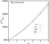
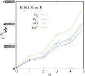
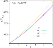
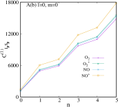
Figure 1: Variation of $C_{I_{\mathrm{\mathbf{r}}}S_{\mathrm{\mathbf{r}}}}^{(1)},~{}C_{I_{\mathrm{\mathbf{p}}}S_{\mathrm{\mathbf{p}}}}^{(1)}$ (bottom row A) and $C_{I_{\mathrm{\mathbf{r}}}S_{\mathrm{\mathbf{r}}}}^{(2)},~{}C_{I_{\mathrm{\mathbf{p}}}S_{\mathrm{\mathbf{p}}}}^{(2)}$ (top row B) in Mie potential with $n$ keeping both $\ell,m$ fixed at zero. Consult text for more details.

Next, Table III reports numerically calculated (from Eq. (18)) $S_{\mathrm{\mathbf{r}}},S_{\mathrm{\mathbf{p}}}$ for the same set of molecules, as in the previous table. The same presentation strategy has been adopted in three horizontal blocks to illustrate changes in $n,\ell,m$ respectively keeping other two fixed at some selected values. From the first block, it is clear that, both measures increase as one goes to higher $n$, for all molecules considered, implying that states become more and more diffused with the addition of radial nodes in wave function. A similar trend is observed in case of $S_{\mathrm{\mathbf{p}}}$ as well. The middle block indicates a reduction in $S_{\mathrm{\mathbf{r}}}$ with progression in $\ell$, whereas $S_{\mathrm{\mathbf{p}}}$ first falls and rises again passing through a minimum, for a chosen molecule. The last block shows that at first they both increase and after reaching maxima they tend to fall off, but the maxima occur at different $m$ in two spaces. An interesting point here is that, in contrast to $I_{\mathrm{\mathbf{r}}}$, $S_{\mathrm{\mathbf{r}}}$ for a neutral molecule assumes higher value than its cationic counterpart. It happens due to the reason that, shifting from neutral to cationic species $D_{0}$ increases and $r_{0}$ decreases. Therefore the latter has a sharp probability distribution (stronger bond) compared to the former. Hence it is evident that an increase in bond strength is indicated by the decrease in $S_{\mathrm{\mathbf{r}}}$. It is worthwhile mentioning that, in all cases, $S_{t}$ obeys the lower bound provided in Eq. (17).

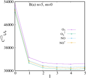
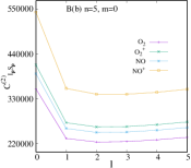
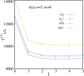
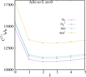
Figure 2: Variation of $C_{I_{\mathrm{\mathbf{r}}}S_{\mathrm{\mathbf{r}}}}^{(1)},~{}C_{I_{\mathrm{\mathbf{p}}}S_{\mathrm{\mathbf{p}}}}^{(1)}$ (bottom row A) $C_{I_{\mathrm{\mathbf{r}}}S_{\mathrm{\mathbf{r}}}}^{(2)},~{}C_{I_{\mathrm{\mathbf{p}}}S_{\mathrm{\mathbf{p}}}}^{(2)}$ (top row B) in Mie potential with $\ell$, choosing $n=5,m=0$. Consult text for more details.

From the foregoing discussion, we see that, at a specific $\ell,m$, both $I_{\mathrm{\mathbf{r}}},S_{\mathrm{\mathbf{r}}}$ escalate with principal quantum number; the former suggesting fluctuation while latter signifying spreading in density distribution. The other state indices have also shown analogous changes in these quantities. Thus it would be interesting to see their combined effect from a consideration of $C_{IS}$, for which we now proceed.

In bottom row panels A(a), A(b) of Fig. 1, $C_{I_{r}S_{r}}^{(1)},C_{I_{p}S_{p}}^{(1)}$ are plotted against $n$ (from 0-5) keeping $\ell,m$ fixed at 0, while $C_{I_{r}S_{r}}^{(2)},C_{I_{p}S_{p}}^{(2)}$ are portrayed in top panels B(a), B(b) respectively. In all four cases, illustrative calculations are done with the same four molecules as earlier. Two segments in first column reveal that, both $C_{I_{r}S_{r}}^{(1)},C_{I_{r}S_{r}}^{(2)}$ grow as $n$ progresses. This can be understood from the data presented in Tables II, III, where we found that both $I,S$ increase with $n$ (for fixed $\ell,m$). Since this implies a rise in number of nodes, it appears that addition of nodes facilitates the system to approach towards disorder. This pattern resembles the Fig. 1(I) in reference shiner99 ; the monotonically increasing function of $n$ indicating a rise in disorder. Similarly for the $p$ space as well, $C_{IS}$ increases with $n$ for both $b$’s but few humps can be noticed. At a given $n$, $C_{I_{r}S_{r}}^{(1)}$ increases from neutral to ionic species; however, this almost coincide for two iso-electronic molecules (O${}_{2}^{+}$, NO). Shifting from neutral to cationic system $r_{0}$ decreases indicating an increase in bond strength with the rise in $I_{\mathrm{\mathbf{r}}}(S_{\mathrm{\mathbf{p}}})$ and a decrease in $S_{\mathrm{\mathbf{r}}}(I_{\mathrm{\mathbf{p}}})$. For $b=\frac{2}{3}$, $I$ dominates over $S$, causing a rise in complexity measure in $r$ space with increasing bond strength. Similar ordering of the neutral and ionic system for a particular state with respect to this complexity measure in $p$ space is observed. In contrast to the former, for $b=1$, $C_{I_{r}S_{r}}^{(2)}$ for neutral molecule possesses higher value than its cationic analogue. This indicates the domination of $S$ over $I$ in the measured quantity while shifting from neutral to cationic equivalent at a particular state. However, in $p$ space, $C^{(2)}_{IS}$ decreases from cation to neutral molecule which is opposite to its conjugate $r$-space ordering. This pattern was lost for $b=\frac{2}{3}$. From this point of view, it seems that $b=1$ possibly qualifies to be a more appropriate descriptor for the systems under investigation.

Similarly, panels A(a), A(b) of the bottom row of Fig. 2 illustrate behaviour of $C_{I_{r}S_{r}}^{(1)}$, $C_{I_{p}S_{p}}^{(1)}$ with changes in $\ell$, while keeping other two quantum numbers $n,m$ fixed at $5,0$ respectively. Analogously, $C_{I_{r}S_{r}}^{(2)}$, $C_{I_{p}S_{p}}^{(2)}$ are pictorially represented in top panels B(a), B(b). Here, both $C_{I_{r}S_{r}}^{(1)},C_{I_{r}S_{r}}^{(2)}$ decline with an increase in $\ell$ having a fixed number of nodes, which acts as an indicator of the system approaching towards disorder. This may be compared to the Fig. 1(III) in reference shiner99 which depicted complexity as a measure of order as decreases with increasing disorder of the system. In $p$ space, both complexity measures first decay, and after reaching a minimal value slightly go up with growth in $\ell$. As noticed in Fig. 1, this figure also supports the fact that $b=1$ possibly characterizes the system in a more appropriate manner. One notices that, while $C_{I_{r}S_{r}}^{(2)}$ and $C_{I_{p}S_{p}}^{(2)}$ show reverse ordering for a particular state in the ionic and neutral species, for $C_{I_{r}S_{r}}^{(1)},C_{I_{p}S_{p}}^{(1)}$ no such reversal occurs.

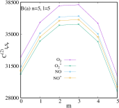
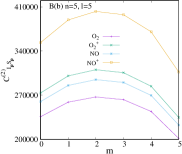
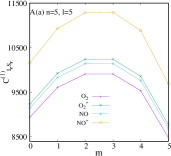
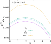
Figure 3: Variation of $C_{I_{\mathrm{\mathbf{r}}}S_{\mathrm{\mathbf{r}}}}^{(1)},~{}C_{I_{\mathrm{\mathbf{p}}}S_{\mathrm{\mathbf{p}}}}^{(1)}$ (bottom row A) and $C_{I_{\mathrm{\mathbf{r}}}S_{\mathrm{\mathbf{r}}}}^{(2)},~{}C_{I_{\mathrm{\mathbf{p}}}S_{\mathrm{\mathbf{p}}}}^{(2)}$ (top row B) in Mie potential with $m$ choosing $n=5,\ell=5$. Consult text for more details.

Finally, Fig. 3 illustrates the nature of $C_{I_{r}S_{r}}^{(1)}$, $C_{I_{p}S_{p}}^{(1)}$ and $C_{I_{r}S_{r}}^{(2)}$, $C_{I_{p}S_{p}}^{(2)}$ with changes in $m$ in panels {A(a), A(b)} and {B(a), B(b)} respectively, keeping $n,\ell$ both fixed at $5$. In both spaces, as $m$ rises, $C_{IS}$ for each molecule gradually increase and after passing through a maximum, falls off. This feature of complexity is a characteristic of the quantum system lying between order and disorder. A similar trend is depicted in Fig. 1(II) of reference shiner99 . Moreover, like earlier two cases, here also $C_{I_{\mathrm{\mathbf{r}}}S_{\mathrm{\mathbf{r}}}}^{(2)}$ possesses larger values for neutral species than ions, but for $C_{I_{\mathrm{\mathbf{p}}}S_{\mathrm{\mathbf{p}}}}^{(2)}$ reverse trend is observed.

IV Concluding Remarks

Information theoretical measures such as $I,~{}S,~{}C_{IS}$ are pursued on some diatomic molecules with generalized Kratzer type potential, in conjugate $r$ and $p$ spaces. These are analyzed in a systematic manner, for both ground and excited states. Exact analytical expressions of $I_{\mathrm{\mathbf{r}}}$ are provided for any given state having arbitrary values for quantum numbers $n,\ell,m$; for $I_{\mathrm{\mathbf{p}}}$ these are derived for only $m=0$ states. Accurate numerical results are presented for four molecules including two cations. Also, an attempt has been made to derive expressions for $S_{\mathrm{\mathbf{r}}}$; however, in this case, only partial analytical expressions have been established in terms of certain entropic integrals. Interesting patterns are observed in the behaviour of $I$ and $S$ in the cationic and neutral molecules. Though both $S$ and $I$ increase with a rise in $n$, the former suggests growth in delocalization while the latter indicates an escalation in fluctuation. With the increase in $\ell$, the variation of both the quantities $I$ and $S$ are consistent in capturing localization. Depending on the choice of quantum numbers ($n,~{}\ell,~{}m$), $C_{IS}$ seems to approach all the three categories mentioned in the reference shiner99 . Furthermore, the investigation of $C_{IS}$ complexity establishes that $b=1$ characterizes the system in a more proper manner than $b=\frac{2}{3}$ for the molecules studied here. It would be interesting to explore other measures like Rényi entropy, Onicescu energy, Tsallis entropy, as well as other complexity measures.

V Acknowledgement

SM is grateful to IISER Kolkata for Junior Research Fellowship (JRF). NM acknowledges SERB-INDIA for National post-doctoral fellowship (sanction order: PDF/2016/000014/CS). Financial support from DST SERB New Delhi, India (sanction order: EMR/2014/000838) is gratefully acknowledged. Constructive comments from two anonymous referees have been very helpful. Prof. A. K. Nanda is thanked for many enlightening discussion.

References

- (1) H. Akcay and R. Sever, J. Math. Chem. 50, 1973 (2012).
- (2) A. R. Matamala, Int. J. Quant. Chem. 89, 129 (2002).
- (3) G. van Hooydonk, Eur. J. Inorg. Chem. 1999, 1617 (1999).
- (4) G. van Hooydonk, Spectrochimica Acta A 56, 2273 (2000).
- (5) A. Kratzer, Z. Phys. 3, 289 (1920).
- (6) E. Fues, Ann. Phys. 80, 367 (1926).
- (7) K. J. Oyewumi, Int. J. Theor. Phys. 49, 1302 (2010).
- (8) I. Bialynicki-Birula and J. Mycielski, Commun. Math. Phys. 44, 129 (1975).
- (9) E. Romera, P. Sànchez-Moreno and J. S. Dehesa, Chem. Phys. Lett. 414, 468 (2005).
- (10) K. D. Sen (Ed.), Statistical Complexity: Applications in Electronic Structure, (Springer, 2012).
- (11) C. Tsallis, J. Stat. Phys. 52, 479 (1988).
- (12) D. Chakraborty and P. W. Ayers, in Statistical Complexity: Applications in Electronic Structure, K. D. Sen (Ed.), pp. 35 (Springer, 2012).
- (13) B. R. Frieden, Science from Fisher Information, Cambridge University Press, (Cambridge, 2004).
- (14) Á. Nagy, J. Chem. Phys. 119, 9401 (2003).
- (15) I. V. Toranzo, P. Sánchez-Moreno, R. O. Esquivel and J. S. Dehesa, Chem. Phys. Lett. 614, 1 (2014).
- (16) Á. Nagy and K. D. Sen, Phys. Lett. A 360, 291 (2006).
- (17) Á. Nagy, Chem. Phys. Lett. 449, 212 (2007).
- (18) R. O. Esquivel, S. Liu, J. C. Angulo, J. S. Dehesa, J. Antolín and M. Molina-Espíritu, J. Phys. Chem. A 115, 4406 (2011).
- (19) S. López-Rosa, R. O. Esquivel, J. C. Angulo, J. Antolín, J. S. Dehesa and N. Flores-Gallegos, J. Chem. Theory Comput. 6, 145 (2010).
- (20) R. F. Nalewajski, Int. J. Quant. Chem. 108, 2230 (2008).
- (21) P. T. Landsberg and J. S. Shiner, Phys. Lett. A 245, 228 (1998).
- (22) J. S. Shiner, M. Davison and P. T. Landsberg, Phys. Rev. E 59, 1459 (1999).
- (23) R. López-Ruiz, H. L. Mancini and X. Calbet, Phys. Lett. A 209, 321 (1995).
- (24) R. G. Catalán, J. Garay and R. López-Ruiz, Phys. Rev. E 66, 011102 (2002).
- (25) J. R. Sánchez and R. López-Ruiz, Physica A 355, 633 (2005).
- (26) E. Romera and J. S. Dehesa, J. Chem. Phys. 120, 8906 (2004).
- (27) K. D. Sen, J. Antolín and J. C. Angulo, Phys. Rev. A 46, 3148 (2007).
- (28) J. C. Angulo, J. Antolín and K. D. Sen, Phys. Lett. A 372, 670 (2008).
- (29) J. S. Dehesa, P. Sánchez-Moreno and R. J. Yáñez, J. Comput. Appl. Math. 186, 523 (2006).
- (30) J. Antolín and J. C. Angulo, Int. J. Quant. Chem. 109, 586 (2009).
- (31) X. Calbet, R. López-Ruiz, Phys. Rev. E 63, 066116 (2001).
- (32) M. T. Martin, A. Plastino and A. O. Rosso, Physica A 369, 439 (2006).
- (33) E. Romera and Á. Nagy, Phys. Lett. A 372, 6823 (2008).
- (34) J. C. Angulo and J. Antolín, J. Chem. Phys. 128, 164109 (2008).
- (35) R. O. Esquivel, J. C. Angulo, J. Antolín, J. S. Dehesa , S. López-Rosa and N. Flores-Gallegos, Phys. Chem. Chem. Phys. 12, 7108 (2010).
- (36) M. A. Welearegay, R. Balawender and A. Holas, Phys. Chem. Chem. Phys. 16, 14928 (2014).
- (37) R. O. Esquivel, M. Molina-Espíritu, J. C. Angulo, J. Antolín, N. Flores-Gallegos and J. S. Dehesa, Mol. Phys. 109, 2353 (2011).
- (38) M. Molina-Espíritu, R. O. Esquivel, J. C. Angulo, J. Antolín and J. S. Dehesa, J. Math. Chem. 50, 1882 (2012).
- (39) R. O. Esquivel, M. Molina-Espíritu, J. S. Dehesa, J. C. Angulo and J. Antolín, Int. J. Quant. Chem. 112, 3578 (2012).
- (40) J. S. Dehesa, A. Martínez-Finkelshtein and V. N. Sorokin, Mol. Phys. 104, 613 (2006).
- (41) S. H. Patil and K. D. Sen, Int. J. Quant. Chem. 107, 1864 (2007).
- (42) P. A. Bouvrie, J. C. Angulo and J. S. Dehesa, Physica A 390, 2215 (2011).
- (43) B. J. Falaye, K. J. Oyewumi, S. M. Ikhdair and M. Hamzavi, Phys. Scr. 89, 115204 (2014).
- (44) S. Dong, G.-H. Sun, S.-H. Dong and J. P. Draayer, Phys. Lett. A 378, 124 (2014).
- (45) W. A. Yahya, K. J. Oyewumi and K. D. Sen, Ind. J. Chem. 53, 1307 (2014).
- (46) D. Nath, Phys. Scr. 89, 065202 (2014).
- (47) W. A. Yahya, K. J. Oyewumi and K. D. Sen, Int. J. Quant. Chem. 115, 1543 (2015).
- (48) G. H. Sun, S. H. Dong, K. D. Launey, T. Dytrych and J. P. Draayer, Int. J. Quant. Chem. 115, 891 (2015).
- (49) X. D. Song, G. H. Sun and S. H. Dong, Phys. Lett. A 379, 1402 (2015).
- (50) B. J. Falaye, K. J. Oyewumi, F. Sadikoglu, M. Hamzavi and S. M. Ikhdair, J. Theor. Comput. Chem. 14, 1550036 (2015).
- (51) W. A. Yahya, K. J. Oyewumi and K. D. Sen, J. Math. Chem. 54, 1810 (2016).
- (52) C. A. Onate and J. O. A. Idiodi, Commun. Theor. Phys. 66, 275 (2016).
- (53) Pooja, R. Kumar, G. Kumar, R. Kumar and A. Kumar, Int. J. Quant. Chem. 116, 1413 (2016).
- (54) J. O. A. Idiodi and C. A. Onate, Commun. Theor. Phys. 66, 269 (2016).
- (55) N. Mukherjee, S. Majumdar and A. K. Roy, Chem. Phys. Lett. 691, 449 (2018).
- (56) N. Mukherjee and A. K. Roy, Int. J. Quant. Chem. e25596 (2018).
- (57) S. Majumdar, N. Mukherjee and A. K. Roy, Chem. Phys. Lett. 687, 322 (2017).
- (58) P. Sánchez-Moreno, R. González-Férez and J. S. Dehesa, New J. Phys. 8, 330 (2006).
- (59) J. S. Dehesa, R. González-Férez and P. Sánchez-Moreno, J. Phys. A 40, 1845 (2007).
- (60) I. S. Gradshteyn and I. M. Ryzhik, Table of integrals, series and products, A. Jeffrey and D. Zwillinger (Eds.), (Academic Press, 2007).
- (61) R. J. Yáñez, W. Van Assche and J. S. Dehesa, Phys. Rev. A 50, 3065 (1994).