A New Approach to Determine Radiative Capture
Reaction Rates at Astrophysical Energies

Abstract

Radiative capture reactions play a crucial role in stellar nucleosynthesis but have proved challenging to determine experimentally. In particular, the large uncertainty ($\sim$100%) in the measured rate of the ¹²C$(\alpha,\gamma)^{16}$O reaction is the largest source of uncertainty in any stellar evolution model. With development of new high current energy-recovery linear accelerators (ERLs) and high density gas targets, measurement of the ¹⁶O$(e,e^{\prime}\alpha)^{12}$C reaction close to threshold using detailed balance opens up a new approach to determine the ¹²C$(\alpha,\gamma)^{16}$O reaction rate with significantly increased precision ($<$20%). We present the formalism to relate photo- and electro-disintegration reactions and consider the design of an optimal experiment to deliver increased precision. Once the new ERLs come online, an experiment to validate the new approach we propose should be carried out. This new approach has broad applicability to radiative capture reactions in astrophysics.

I Introduction.

Radiative capture reactions, i.e., nuclear reactions in which the incident projectile is absorbed by the target nucleus and $\gamma$-radiation is then emitted, play a crucial role in nucleosynthesis processes in stars Rolfs and Barnes (1990). For example, knowledge of their reaction rates at stellar energies is essential to understanding the abundance of the chemical elements in the universe. However, determination of these reaction rates has proven to be challenging, principally due to the Coulomb repulsion between initial-state nuclei and the weakness of the electromagnetic force. For example, the decay of unbound nuclear states by the emission of a particle of the same type as that captured, or by the emission of some other type of particle, is often $10^{3}-10^{6}$ times more probable than decay by $\gamma$-emission.

In stellar nucleosynthesis, at the completion of the hydrogen burning stage, the core of a massive star contracts and heats-up. When the temperature and the density of the core reaches sufficiently high values, the helium starts to burn via the triple-$\alpha\rightarrow$ ¹²C process. Subsequently, the $\alpha$ radiative capture reaction ¹²C$(\alpha,\gamma)^{16}$O also becomes possible. The helium burning stage is fully dominated by these two reactions and their rates determine the relative abundance of ¹²C and ¹⁶O, after the helium is depleted. At helium burning temperatures, the rate of the triple-$\alpha$ process is known with an uncertainty of about $\pm$10%, but the uncertainty of the ¹²C$(\alpha,\gamma)^{16}$O reaction rate is much larger. In fact, it is the largest source of uncertainty in any stellar evolution model. Therefore, for many decades it has been the paramount experimental goal of nuclear astrophysics to determine the rate of ¹²C$(\alpha,\gamma)^{16}$O reaction at astrophysical energies with better precision Woosley et al. (2003).

This task has been proven to be very difficult, not withstanding heroic experimental efforts for more than half a century. For the generic radiative capture reaction

$$A+B\rightarrow C\rightarrow D+\gamma\ ,$$ (1)

the Coulomb repulsion is characterized by the Gamow factor (or Coulomb barrier penetration factor) between $A$ and $B$

$$P_{g}=\exp{-\sqrt{E_{g}/E}}\ ,$$ (2)

where $E_{g}\equiv 2m_{r}c^{2}(\pi\alpha Z_{A}Z_{B})^{2}$ is the Gamow energy and $m_{r}=\frac{m_{A}m_{B}}{m_{A}+m_{B}}$ is the reduced mass. The cross section $\sigma$ is then expressed Donnelly et al. (2017) as a product of $P_{g}$ and the astrophysical S-factor

$$\sigma\equiv\frac{1}{E}\exp{[-2\pi Z_{A}Z_{B}\alpha/v]}S(E)\ .$$ (3)

$\sigma$ is further extrapolated to the Gamow energy, which is representative of stellar energies.

At the helium burning temperature $\sim 2\times 10^{8}$ K and corresponding Gamow energy $E_{g}\sim 300$ keV, the cross section for the ${}^{12}C+\alpha\rightarrow\gamma+{}^{16}O$ reaction is $\approx 10^{-5}$ pb, which makes the direct measurement at stellar energies impossible. Unfortunately, the extrapolation is not simple, since the structure of the cross section is complex. It involves interference of the high-energy tail of the $J^{\pi}=1^{-}$ subthreshold state in ¹⁶O (see Tilley et al. (1993)) at $7.12$ MeV and the broad $1^{-}$ resonance at $9.59$ MeV, and interference of the subthreshold state $2^{+}$ at $6.92$ MeV and the narrow $2^{+}$ resonance at $9.85$ MeV. Additionally, cascade transitions to the ground state of ¹⁶O need to be taken into account as well as the direct capture for the E2 amplitude.

Through the years, different experimental approaches have been used to determine the rate of the ¹²C$(\alpha,\gamma)^{16}$O reaction. These include measurements of the direct reaction Dyer and Barnes (1974); Redder et al. (1987); Kremer et al. (1988); Ouellet et al. (1996); Roters et al. (1999); Gialanella et al. (2001); Kunz et al. (2001); Kunz (2002); Fey (2004); Schürmann et al. (2005); Assunção et al. (2006); Makii et al. (2009); Schürmann et al. (2011); Plag et al. (2012), $\beta-$delayed $\alpha$-decay of ¹⁶N Buchmann et al. (1993); Azuma et al. (1994); Tang et al. (2010) and elastic scattering ¹²C$(\alpha,\alpha)^{12}$C Plaga et al. (1987); Tischhauser et al. (2009). As described below, we have fit the world’s data in the region $0.7\leq E_{\alpha}^{c.m.}\leq 1.7$ MeV, for both multipoles, where $E_{\alpha}^{c.m.}$ is the kinetic energy of the $\alpha$-particle in the center-of-mass ($c.m.$) of the ¹²C$-\alpha$ system. The resulting $S_{EJ}(E_{\alpha}^{c.m.})$ dependence was approximated by fitting the data to second-order polynomials, which are represented by the dashed curves in Fig. 1.

However, due to the rapid decrease of the cross section in the region where $E_{\alpha}^{c.m.}$ falls below 2 MeV, the uncertainty in the S-factor experimental determination is increasingly dominated by the large statistical uncertainty. Further, as $E_{\alpha}^{c.m.}$ decreases, the statistical uncertainties from the different experiments increase rapidly. A comprehensive review of the experiments and methods developed so far, and the full list of astrophysical implications of the ¹²C$(\alpha,\gamma)^{16}$O rate can be found in deBoer et al. (2017).

In recent years, there have been new experimental approaches pursued. One novel approach is based on a bubble chamber detector DiGiovine et al. (2015) where the number of photodisintegrations is counted and the total astrophysical $S$-factor could be measured even at very low energies Holt et al. (2018). However, the isotopic impurities of ¹⁷O and ¹⁸O have to be greatly suppressed Ugalde et al. (2013). Another ¹⁶O photodisintegration experiment is based on the optical time projection chamber Gai et al. (2010) where the angular distribution of $\alpha$-particles is measured and the $S_{E1}$- and $S_{E2}$-factors can be determined. This approach works well for higher $\alpha$-particle energies, but for lower energies the density of the gas needs to be reduced.

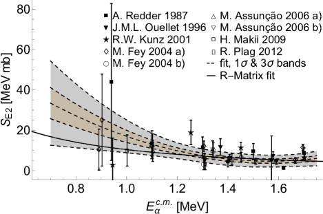
Figure 1: Measured astrophysical $S_{E1}$- and $S_{E2}$-factors for $E_{\alpha}<1.7$ MeV from Dyer and Barnes Dyer and Barnes (1974), A. Redder Redder et al. (1987), R. M. Kremer Kremer et al. (1988), J. M. L. Ouellet Ouellet et al. (1996), G. Roters Roters et al. (1999), R. W. Kunz Kunz et al. (2001); Kunz (2002), L. Gialanella Gialanella et al. (2001), M. Fey a) turning table measurement and b) EUROGAM measurement Fey (2004), M. Assunção a) two parameters fit and b) three parameters fit Assunção et al. (2006), H. Makii Makii et al. (2009) and R. Plag Plag et al. (2012). An R-Matrix fit to the data, represented by the solid line, was performed using the AZURE2 code Azuma et al. (2010).

In this paper, we present in some detail a new approach to the determination of radiative capture reactions at stellar energies. We consider the inverse reaction initiated by an electron beam rather than a photon beam. The idea has been previously proposed Tsentalovich et al. (2000), but not measured, and more recently discussed by Friščić (2017); Lunkenheimer (2017). The theoretical formalism to relate electro- and photo-disintegration has been developed Raskin and Donnelly (1989). Most importantly, a new generation of high intensity ($\approx$ 10 mA) low-energy ($\approx$ 100 MeV) energy-recovery linear (ERL) electron accelerators is under development Hug et al. (2017); Hoffstaetter et al. (2017) which, when used with state-of-the-art gas targets Grieser et al. (2018), can deliver luminosities of $\approx 10^{36}$ cm^-2 s^-1 for experiment MIT . In this way, the weakness of the electromagnetic force can be overcome. Here, we have chosen to focus specifically on determination of the reaction rate of ¹²C$(\alpha,\gamma)^{16}$O at stellar energies using this new approach. However, our approach is generally applicable to all radiative capture reactions.

To provide a basis for the theory used to make estimations of event rates for the electrodisintegration reaction we have begun by revisiting what is typically done for photodisintegration. In the latter case, shell model or cluster model approaches have had some degree of success in yielding the general shape of the cross section, but fail to get its overall magnitude correct. On the one hand, since the electrodisintegration cross section demands even more of any modeling — specifically, not only the energy dependence of the cross section, but also its momentum transfer behavior (see the following section) — at present one cannot depend on typical modeling to provide reliable estimates of the cross section. On the other hand, our focus is on very low energies (typically within an MeV or so of threshold) and relatively low momentum transfers (much smaller than a characteristic nuclear value of 200-300 MeV/c). This means that the form of the cross section as a function of the momentum transfer is tightly constrained. Indeed, as we show in the following sections, the momentum transfer dependence of the cross section can be characterized by a small number of constants, and, importantly, these few constants can be determined experimentally by making measurements at several values of the momentum transfer. In effect, at present it is possible to make reasonable estimates of the electrodisintegration cross section despite the lack of a satisfactory detailed model. Of course, our parametrization of the cross section has been designed to recover what is presently known about the photodisintegration cross section, namely, what must be recovered for the electrodisintegration cross section in the real-photon limit, as discussed in the next section.

We have considered the optimal experimental kinematics in terms of the incident electron energy, the oxygen gas target, the scattered electron spectrometer, and the final-state, low-energy $\alpha$-particle detection. We have considered systematic uncertainties such as both isotopic and chemical contamination of the ¹⁶O; energy, angle and timing constraints of the final-state particles; energy loss in the gas jet and radiative corrections. Using realistic experimental assumptions, we propose an initial measurement of ¹⁶O$(e,e^{\prime}\alpha){}^{12}$C using an ERL with incident energy of order 100 MeV. The experiment would take data at higher $E_{\alpha}^{c.m.}$ where the reaction rates are relatively high and the running time is of order a month. This initial measurement would aim to validate the extrapolation to photodisintegration and determine the contributions of different multipoles. If successful, it would set the stage for a longer experiment (of order 6 months) with the highest electron intensity available to determine the ¹²C$(\alpha,\gamma)^{16}$O reaction rate with unprecedented precision in the astrophysical region.

In Sect. II, the general relationship between electro- and photo-induced reactions is presented, while in Sect. III, following the general formalism presented in Raskin and Donnelly (1989), these developments are applied to the exclusive ¹⁶O$(e,e^{\prime}\alpha)^{12}$C(g.s.) process in which all nuclear species have $J^{\pi}=0^{+}$. In Sect. IV the multipole decomposition of the response functions involved is discussed, truncating the set of multipoles at the quadrupole response, and thus including C0, C1/E1 and C2/E2 multipoles. Following this general discussion, in Sect. V the model adopted for the semi-inclusive electrodisintegration cross section is presented. Specifically, in Sect. V.1 the present knowledge from studies of photodisintegration and radiative capture reactions is employed in a determination of the leading-order behavior of the C1/E1 and C2/E2 multipoles. Following this, in Sect. V.2 our way of treating the next-to-leading order coefficients in expansions in $q$ is discussed, together with the approach taken for the C0 multipole. Section V.3 concludes the discussion of the model with presentations of the electrodisintegration cross section for typical choices of kinematics in the desired low-$\omega$/low-$q$ region. Given the model, Sect. VI then continues with the central section of this paper in which it is shown that, by making assumptions concerning the experimental capabilities that are projected to exist in the not-too-distant future, measurements of electrodisintegration of ¹⁶O appear to be feasible and that such measurements can be employed to significantly reduce the statistical uncertainties of the $S_{E1}$- and $S_{E2}$-factors in the $E_{\alpha}^{c.m.}<2$ MeV region. Additionally, in that section a discussion of how a smart choice of observable should allow one not only to identify the final-state $\alpha$, but also to identify and remove background events such as $\alpha$-particles from electrodisintegration of other oxygen isotopes (¹⁷O and ¹⁸O) or other ions emerging from electrodisintegration of impurities found in an oxygen gas target, e.g., protons from ¹⁴N$(e,e^{\prime}p)^{13}$C. We conclude with a summary and a perspective on the future in Section VII.

II Relationships between Photo- and Electro-disintegration

We begin with a brief discussion of how studies of photodisintegration can be extended to those of electrodisintegration, focusing on the disintegration of ¹⁶O into the ground states of ⁴He (the $\alpha$ particle) and ¹²C. For the reader who is unfamiliar with the basic formalism that relates the two processes we can recommend the recent book involving two of the authors Donnelly et al. (2017), in particular Chapters 7 and 16, including references therein.

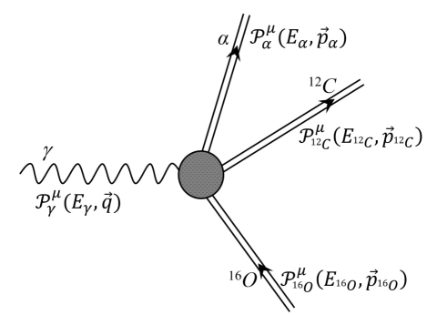
Figure 2: Feynman diagram for the photodisintegration of ¹⁶O involving a real photon, $\gamma$, which requires that $q=\omega=E_{\gamma}$. The kinematic variables here will be discussed in more detail in Sect. III.

As discussed above, studies aimed at determinations of the alpha + carbon capture reaction ¹²C$(\alpha,\gamma)^{16}$O have made use of the inverse process, namely the photodisintegration of oxygen, ¹⁶O$(\gamma,\alpha)^{12}$C, together with detailed balance. In the present work we describe an extension of these ideas by focusing on the electrodisintegration reaction ¹⁶O$(e,e^{\prime}\alpha)^{12}$C. Both photo- and electro-disintegration reactions are assumed to be exclusive, i.e., to have the $\alpha$-particle in the final state detected. However, they differ in that the former involves real photons whose momenta $q$ must be equal to their energies $\omega=E_{\gamma}$, corresponding to so-called real-photon kinematics, as illustrated in Fig. 2. In contrast, as illustrated in Fig. 3, in the one-photon-exchange approximation, which is generally good at the percent level for light nuclei, the latter involves virtual photon exchanges that may be shown to be spacelike, $q>\omega$. That is, by knowing the electron scattering kinematics it is possible to focus on a specific value of the excitation energy of the final-state $\alpha+^{12}$C system, for instance quite close to threshold, but to vary the three-momentum transfer $q$ for any value that keeps the exchanged virtual photon spacelike. Of course, the real-photon result is recovered by taking the limit where $q\to\omega$.

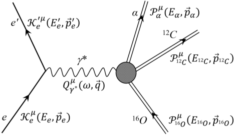
Figure 3: First-order Feynman diagram for the electrodisintegration of ¹⁶O involving one virtual photon $\gamma\text{*}$ exchange, to be compared with Fig. 2. Again, the kinematic variables here will be discussed in more detail in Sect. III.

A sketch of the general landscape is given in Fig. 4 which illustrates a typical response (see later sections of the present work for specifics) as a function of $q$ and $\omega$ together with the real-$\gamma$ line; here $\omega_{th}$ is the threshold value of $\omega$ for the reaction. The strategy in photodisintegration studies is to perform experiments at values of $\omega=E_{\gamma}$ where the cross section is large enough to be measured and then extrapolate along the real-$\gamma$ line to the very low energies of interest for astrophysics. The electrodisintegration reaction extends these ideas: now one can focus on small values of $\omega$ but have $q$ large enough to yield measurable cross sections. The extended strategy is then to extrapolate in both dimensions, namely, for the responses as functions of $q$ to approach the real-$\gamma$ line and as functions of $\omega$ to reach the interesting low-energy region. As will be discussed in the following sections, an advantage of having $q$ large enough is that one may work near threshold but have sufficient three-momentum imparted to the $\alpha$-particles in the final state that they can emerge from the target and be detected.

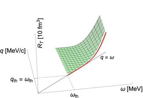
Figure 4: Transverse response function $R_{T}$ as function of the photon energy $\omega$ and the three-momentum transfer $q$, for the real photon case $q=\omega$ (solid line) and virtual photon case $q>\omega$ (surface plot), where $\omega_{th}$ denotes the value of the threshold photon energy for the reaction.

Both photo- and electro-disintegration reactions have in common that the angular distribution of the $\alpha$-particles in the final state can be measured. This yields information on the various multipoles that contribute to the process. We assume that $\omega$ is always quite small compared with a typical energy scale; in addition, for the electrodisintegration reaction we assume that $q$ is smaller than a typical scale for nuclear momenta, $q_{0}$, taken to be roughly of order 200–250 MeV/c. Given this, it is possible to limit the multipoles to a relatively small number. This is commonly done for the photodisintegration reaction near threshold where only $E1$ (electric dipole) and $E2$ (electric quadrupole) multipoles are assumed, although one can ask how important electric octupole $E3$ multipoles might be. Since the nuclear ground states involved are all $0^{+}$ states only electric multipoles can occur, and magnetic multipoles are absent. Here we have assumed that only the ground states of ⁴He and ¹²C are involved and that any excited states can be ignored by using the over-determined kinematics of the reaction. The electrodisintegration reaction is richer, as will be discussed in detail in the following sections of the paper. Since virtual photons are involved, now one has Coulomb $CJ$ as well as electric multipoles $EJ$; in the body of the paper we consider $C0$, $C1/E1$ and $C2/E2$ multipoles, although in an appendix we give some of the relevant formalism for a larger set that includes $C3/E3$ contributions.

At low values of the momentum transfer, $q\ll q_{0}$, each multipole is dominated by its low-$q$ behavior which enters as a specific power of $q$. For instance, later we show that the $CJ$ mulipole matrix elements go as $(q/q_{0})^{J}$ at low $q$. Accordingly another advantage of electron scattering where $q$ may be varied while keeping $\omega$ fixed is that the balance of the multipole contributions can be varied. An example of this could, for instance, be the potential $C3/E3$ contributions: by increasing $q$ (still, of course, staying in the region where $q\ll q_{0}$) one may increase the relative importance of the octupole effects over the monopole, dipole and quadrupole effects to explore whether or not the former need to be taken into account.

Not only is there a richer set of mutipoles involved in the electron scattering case, but there are more response functions to be exploited. For real photons one has the transverse response $R_{T}$ at $q=\omega$ and potentially the transverse interference response $R_{TT}$ also at $q=\omega$ if linearly polarized real photons are involved (see Sect. III for more discussion). For unpolarized electron scattering there are four types of responses, $R_{T}$ and $R_{TT}$ as for real photons but now with virtual photons and thus at $q>\omega$ and also $R_{L}$, the longitudinal/charge response and an interference between transverse and longitudinal contributions, $R_{TL}$, both at $q>\omega$. In the $R_{T}$ and $R_{TT}$ responses only $EJ$ multipoles enter, not simply squared but through interferences. The $R_{L}$ response contains only $CJ$ multipoles, again with interferences, while the $R_{TL}$ response has interferences between $CJ$ and $EJ$ mutipoles. All of this means that potentially one has more information with which to disentangle the various contributions. The angular distributions as functions of the alpha angles $\theta_{\alpha}$ and $\phi_{\alpha}$ (see the next section) will be discussed in detail. These may be written as expansions in terms of Legendre polynomials where the expansion coefficients that enter and may be determined experimentally contain valuable information on all bilinear products of the multipole matrix elements.

We now proceed to a summary of the kinematics and basic form of the semi-inclusive electron scattering cross section in the following section.

III Kinematics and the cross section

We start this section with a brief discussion of exclusive-1 electron scattering A$(e,e^{\prime}x)$, following Raskin and Donnelly (1989), although, in contrast to the more general study in Raskin and Donnelly (1989), here the discussion will be limited to the scattering of unpolarized electrons from an unpolarized target nucleus, i.e., polarization degrees of freedom will be neglected. We limit our consideration to the one-photon exchange contributions (lowest order, see Fig. 3), and take the electron wave functions to be plane waves, namely, we invoke the plane-wave Born approximation (PWBA). The four-momenta of the incident and scattered electrons are labeled $\mathcal{K}^{\mu}_{e}(E_{e},\vv{p}_{\mkern-4.0mue})$ and $\mathcal{K^{\prime}}^{\mu}_{\mkern-6.0mue}(E^{\prime}_{e},\vv{p}^{\prime}_{\mkern-4.0mue})$, respectively. $E_{e}$ and $E^{\prime}_{e}$ are their energies, while $\vv{p}_{\mkern-4.0mue}$ and $\vv{p}^{\prime}_{\mkern-4.0mue}$ are their three-momenta. The four-momentum transfer is defined by $Q^{\mu}\equiv(\omega,\vv{q})=\mathcal{K}^{\mu}_{e}-\mathcal{K^{\prime}}^{\mu}_{\mkern-6.0mue}=\mathcal{P}^{\mu}_{{}^{16}O}-\mathcal{P}^{\mu}_{{}^{12}C}-\mathcal{P}^{\mu}_{\alpha}$, where $\mathcal{P}^{\mu}_{{}^{16}O}$, $\mathcal{P}^{\mu}_{{}^{12}C}$ and $\mathcal{P}^{\mu}_{\alpha}$ are the four-momenta of the target nucleus ¹⁶O, residual nucleus ¹²C and exclusive nucleus $\alpha$. Also, $\omega=E_{e}-E^{\prime}_{e}=E_{\alpha}+E_{{}^{12}C}-E_{{}^{16}O}$ is the energy transfer and $\vv{q}=\vv{p}_{\mkern-4.0mue}-\vv{p}^{\prime}_{\mkern-4.0mue}=\vv{p}_{\mkern-3.0mu\alpha}+\vv{p}_{\mkern-3.0mu{}^{12}C}-\vv{p}_{\mkern-3.0mu{}^{16}O}$ is the three-momentum transfer.

In order to identify the events belonging to the electrodisintegration of ¹⁶O a scattered electron needs to be detected in coincidence with a produced $\alpha$-particle and the four-momenta of both have to be measured. The remaining ¹²C nucleus does not need to be detected, since its final state can be reconstructed by using energy-momentum conservation. The variables typically used to characterize the semi-inclusive reaction are the following (see Donnelly et al. (2017)): the missing momentum $\vv{p}_{miss}$ and missing energy $E_{miss}$ are given by

$$\vv{p}_{miss} =\vv{q}-\vv{p}_{\alpha}$$ (4)

$$E_{miss} =\omega+M_{{}^{16}O}-E_{\alpha},$$ (5)

and then the missing mass

$$m_{miss}=\sqrt{E_{miss}^{2}-\vv{p}_{miss}^{2}}$$ (6)

may be calculated by subtracting the mass of the unobserved ¹²C nucleus, $M_{{}^{12}C}$. One then obtains the excitation energy of the ¹²C,

$$E_{ex}=m_{miss}-M_{{}^{12}C},$$ (7)

where events which contribute to the astrophysical $S$-factor are those where one finds the ¹²C nucleus in its ground state, that is, $E_{ex}=0$.

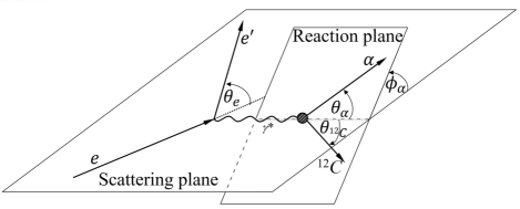
Figure 5: Kinematics of the exclusive ¹⁶O$(e,e^{\prime}\alpha)^{12}$C reaction.

The differential cross section in laboratory frame (where the target is at rest, $\mathcal{P}^{\mu}_{{}^{16}O}=(M_{{}^{16}O},0)$) is given by Bjorken and Drell (1964)

$$d\sigma=\frac{m_{e}}{E_{e}}\frac{1}{\beta_{e}}\overline{\sum\limits_{fi}}|\mathcal{M}_{fi}|^{2}\frac{m_{e}}{E^{\prime}_{e}}\frac{d^{3}\vv{p}_{e}^{\prime}}{(2\pi)^{3}}\frac{M_{\alpha}}{E_{\alpha}}\frac{d^{3}\vv{p}_{\mkern-3.0mu\alpha}}{(2\pi)^{3}}\frac{M_{{}^{12}C}}{E_{{}^{12}C}}\frac{d^{3}\vv{p}_{\mkern-3.0mu{}^{12}C}}{(2\pi)^{3}}(4\pi)^{4}\delta^{4}(\mathcal{K}^{\mu}_{e}+\mathcal{P}^{\mu}_{\mkern-3.0mu{}^{16}O}-\mathcal{K^{\prime}}^{\mu}_{\mkern-6.0mue}-\mathcal{P}^{\mu}_{\alpha}-\mathcal{P}^{\mu}_{{}^{12}C}),$$ (8)

where $\beta_{e}=|\vv{p}_{e}|/E_{e}=|\vv{v}_{e}|$ and $\overline{\sum}_{fi}$ represents an average over initial states and sum over final states, under the assumption that all particle states are normalized to unity. If we assume the momenta of the scattered electron and $\alpha$-particle to be measured but not the residual ¹²C nucleus, we need to perform an integration over the recoil momentum $\vv{p}_{\mkern-3.0mu{}^{12}C}$:

$$d\sigma=\frac{m_{e}^{2}M_{\alpha}M_{{}^{1}2{C}}}{E_{e}}\frac{1}{(2\pi)^{5}}\overline{\sum\limits_{fi}}|\mathcal{M}_{fi}|^{2}\frac{p^{\prime 2}_{e}dp^{\prime}_{e}d\Omega_{e}p^{2}_{\alpha}dp_{\alpha}d\Omega_{\alpha}}{E^{\prime}_{e}E_{\alpha}E_{{}^{12}C}}\delta(E_{e}+E_{{}^{16}O}-E^{\prime}_{e}-E_{\alpha}-E_{{}^{12}C}).$$ (9)

We continue to integrate the energy-conserving delta-function of energy conservation over $p_{\alpha}$ and make use of the following formula

$$\delta(f(p))=\sum\limits_{i}\cfrac{\delta(p-p_{i})}{\bigg{|}\cfrac{\partial f(p)}{\partial p}\bigg{|}_{p_{i}}},$$ (10)

where $f(p_{i})=0$ and

$$f(p_{\alpha})=\omega+M_{{}^{16}O}-\sqrt{|\vv{p}_{\mkern-3.0mu\alpha}|^{2}+M^{2}_{\alpha}}-\sqrt{(\vv{q}-\vv{p}_{\mkern-3.0mu\alpha})^{2}+M^{2}_{{}^{12}C}}.$$ (11)

After the integration we obtain

$$\int \frac{p^{2}_{\alpha}dp_{\alpha}}{E_{\alpha}E_{{}^{12}C}}\delta(E_{e}+E_{{}^{16}O}-E^{\prime}_{e}-E_{\alpha}-E_{{}^{12}C})$$

$$=\frac{p_{\alpha}}{M_{{}^{16}O}}\cfrac{1}{\bigg{|}1+\cfrac{\omega p_{\alpha}-E_{\alpha}|\vv{q}|\cos\theta_{\alpha}}{M_{{}^{16}O}\cdot p_{\alpha}}\bigg{|}}$$

$$=\frac{p_{\alpha}}{M_{{}^{16}O}}f_{rec}^{-1},$$ (12)

where $f_{rec}$ is the hadronic recoil factor and $\theta_{\alpha}$ is the angle between $\vv{q}$ and $\vv{p}_{\alpha}$; see Fig 5. The cross section is now

$$d\sigma=\frac{m_{e}^{2}M_{\alpha}M_{{}^{12}C}}{(2\pi)^{5}M_{{}^{16}O}}\frac{E^{\prime}_{e}\cdot p_{\alpha}}{E_{e}}f_{rec}^{-1}\overline{\sum\limits_{fi}}|\mathcal{M}_{fi}|^{2}.$$ (13)

The Lorentz-invariant matrix element $\mathcal{M}_{fi}$ is given by

$$\mathcal{M}_{fi}=\frac{ie}{Q^{2}}\Bigg{(}\frac{E_{e}E^{\prime}_{e}}{m^{2}_{e}}\Bigg{)}^{\frac{1}{2}}j_{e}(\mathcal{K^{\prime}}_{\mkern-6.0mue},\mathcal{K}_{e})_{\mu}J^{\mu}(\mathcal{P}_{{}^{12}C},\mathcal{P}_{\alpha};\mathcal{P}_{{}^{16}O})_{fi},$$ (14)

where $j_{e}(\mathcal{K^{\prime}}_{\mkern-6.0mue},\mathcal{K}_{e})_{\mu}$ is the electromagnetic electron current, $J^{\mu}(\mathcal{P}_{{}^{12}C},\mathcal{P}_{\alpha};\mathcal{P}_{{}^{16}O})_{fi}$ is the hadronic electromagnetic transition current and the square of the four-momentum transfer in the extreme relativistic limit (ERL) is given by $|Q^{2}|=4E_{e}E^{\prime}_{e}\sin^{2}(\theta_{e}/2)$, where $\theta_{e}$ is the electron scattering angle; see Fig. 5. When we square $\mathcal{M}_{fi}$, sum over final states and average over initial states, we end up with

$$\overline{\sum\limits_{fi}}|\mathcal{M}_{fi}|^{2}=\frac{(4\pi\alpha)^{2}}{(Q^{2})^{2}}\eta_{\mu\nu}W^{\mu\nu},$$ (15)

where $\eta_{\mu\nu}$ is the leptonic tensor and $W^{\mu\nu}$ is the hadronic tensor. Note that the contraction of the leptonic and hadronic tensors is Lorentz invariant. Accordingly it can be evaluated in any frame and it is given by

$$\eta_{\mu\nu}W^{\mu\nu}=\frac{v_{0}}{4m_{e}^{2}}\sum\limits_{K}v_{K}R_{K}$$ (16)

with $v_{0}=4E_{e}E^{\prime}_{e}\cos^{2}(\theta_{e}/2)$. For the unpolarized exclusive electron scattering we have four nuclear response functions $R_{K}$: the longitudinal $R_{L}$ and transverse $R_{T}$ nuclear electromagnetic current components (longitudinal and transverse with respect to the direction of the virtual photon $\vv{q}$), and two interference responses, namely transverse-longitudinal $R_{TL}$ and transverse-transverse $R_{TT}$. In this notation $R_{K}$ will have dimension of fm³. The functions $v_{K}$ are electron kinematic factors and in terms of ERL can be expressed as Raskin and Donnelly (1989)

$$v_{L} =\rho^{2}$$

$$v_{T} =\frac{1}{2}\rho+\tan^{2}\theta_{e}/2$$

$$v_{TL} =-\frac{1}{\sqrt{2}}\rho\sqrt{\rho+\tan^{2}\theta_{e}/2}$$

$$v_{TT} =-\frac{1}{2}\rho,$$ (17)

where as usual $0\leq\rho\equiv|Q^{2}/q^{2}|=1-(\omega/q)^{2}\leq 1$. The most general discussion concerning the leptonic and hadronic tensor contraction, which also includes polarization degrees of freedom, can be found in Raskin and Donnelly (1989); Donnelly and Raskin (1986).

It is convenient to group variables to form the ERL Mott cross section

$$\sigma_{Mott}=\frac{\alpha^{2}(\hbar c)^{2}E^{\prime}_{e}v_{0}}{(Q^{2})^{2}E_{e}}=\bigg{(}\frac{\alpha\hbar c\cos\theta_{e}/2}{2E_{e}\sin^{2}\theta_{e}/2}\bigg{)}^{2}.$$ (18)

Note that here we include the factor $\hbar c=197.327$ MeV ​fm so that $\sigma_{Mott}$ has dimensions of fm². Finally, the semi-inclusive electrodisintegration cross section for the reaction of interest in the laboratory frame takes the form

$$\Bigg{[}\frac{d\sigma}{d\omega d\Omega_{e}d\Omega_{\alpha}}\Bigg{]}_{(e,e^{\prime}\alpha)}=\frac{M_{\alpha}M_{{}^{12}C}}{8\pi^{3}M_{{}^{16}O}}\frac{p_{\alpha}f^{-1}_{rec}\sigma_{Mott}}{(\hbar c)^{3}}\bigg{(}v_{L}R_{L}+v_{T}R_{T}+v_{TL}R_{TL}+v_{TT}R_{TT}\bigg{)}.$$ (19)

Often it also very convenient to have an expression for the cross section in the center-of-mass ($c.m.$) frame, where the transformation between the frames involves a Lorentz boost along $\vv{q}$. We note that $W=\sqrt{(M_{{}^{16}O}+\omega)^{2}-q^{2}}$ is the total invariant mass of the $\gamma+^{16}$O and $\alpha+^{12}$C systems, here evaluated in the incident channel laboratory frame with the ¹⁶O target nucleus at rest. Furthermore, $p^{c.m.}_{\alpha}=|\vv{p}\;^{c.m.}_{\alpha}|$ is the $\alpha$-particle three-momentum in the $c.m.$ frame, $R_{K}$ now represent quantities in the $c.m.$ frame and the lepton kinematic factors in the $c.m.$ frame are given by the following:

$$\widetilde{v}_{L} =(W/M_{{}^{16}O})^{2}v_{L},$$

$$\widetilde{v}_{TL} =(W/M_{{}^{16}O})v_{T},$$

$$\widetilde{v}_{T} =v_{T},$$

$$\widetilde{v}_{TT} =v_{TT}.$$ (20)

Finally, the cross section in the $c.m.$ frame can be written as

$$\Bigg{[}\frac{d\sigma}{d\omega d\Omega_{e}d\Omega^{c.m.}_{\alpha}}\Bigg{]}_{(e,e^{\prime}\alpha)}=\frac{M_{\alpha}M_{{}^{12}C}}{8\pi^{3}W}\frac{p^{c.m.}_{\alpha}\sigma_{Mott}}{(\hbar c)^{3}}\bigg{(}\widetilde{v}_{L}R_{L}+\widetilde{v}_{T}R_{T}+\widetilde{v}_{TL}R_{TL}+\widetilde{v}_{TT}R_{TT}\bigg{)}.$$ (21)

Note that $\phi_{\alpha}=\phi_{\alpha}^{c.m.}$, although $\theta_{\alpha}\neq\theta_{\alpha}^{c.m.}$. Again, we encourage the reader who is unfamiliar with these developments to look at Donnelly et al. (2017), especially Chapter 7 where the current matrix elements are discussed, multipole operators are introduced and the real-photon limit is briefly treated, as well as Chapter 16 where semi-inclusive electron scattering is the focus (there one also finds Exercises 16.4, 16.6 and 16.7 which are relevant for the present purposes, especially Exercise 16.7 where a problem involving the real-photon limit of semi-inclusive electron scattering is posed).

An analysis similar to the one in Raskin and Donnelly (1989) can be performed both for the photodisintegration process ¹⁶O$(\gamma,\alpha)^{12}$C and for the radiative capture reaction ¹²C$(\alpha,\gamma)^{16}$O, where here for simplicity we take the real photons to be unpolarized (see the comment regarding linearly polarized photons in the next section). For the former reaction the differential cross section is given by

$$\Bigg{[}\frac{d\sigma}{d\Omega^{c.m.}_{\alpha}}\Bigg{]}_{(\gamma,\alpha)}=\Bigg{(}\frac{M_{\alpha}M_{{}^{12}C}}{4\pi W}\Bigg{)}\frac{p^{c.m.}_{\alpha}}{\hbar c}\Bigg{(}\frac{\alpha}{E_{\gamma}}\Bigg{)}\mathcal{R}_{(\gamma,\alpha)},$$ (22)

where $W=\sqrt{M_{{}^{16}O}(M_{{}^{16}O}+2E_{\gamma})}$ (that is, $q=\omega=E_{\gamma}$ above) and $\mathcal{R}_{(\gamma,\alpha)}$ is transverse response function having dimension of fm³. Namely, one has the real-photon limit of the electrodisintegration result summarized above. The radiative capture cross section is then related by detailed balance and may be written in the form

$$\Bigg{[}\frac{d\sigma}{d\Omega^{c.m.}_{\gamma}}\Bigg{]}_{(\alpha,\gamma)}=\Bigg{(}\frac{M_{\alpha}M_{{}^{12}C}}{2\pi W}\Bigg{)}\frac{E_{\gamma}}{\hbar c}\Bigg{(}\frac{\alpha}{p^{c.m.}_{\alpha}}\Bigg{)}\mathcal{R}_{(\alpha,\gamma)},$$ (23)

where $W$ is the invariant mass above, which, in the incident channel laboratory frame where the ¹²C target is at rest, is equal to $W=\sqrt{M^{2}_{\alpha}+M^{2}_{{}^{12}C}+2M_{{}^{12}C}E^{Lab}_{\alpha}}$. As above, $\mathcal{R}_{(\alpha,\gamma)}$ is the transverse response function, here for real photons to be evaluated at $q=\omega=E_{\gamma}$; it has dimensions of fm³.

IV Multipole decomposition of response functions involving spin $\bf 0$ nuclei

Let us discuss the longitudinal-transverse decomposition a little further. For the specific initial and final nuclear states involved there are three independent current matrix elements, $\rho(\vv{q})$, $J^{x}(\vv{q})$ and $J^{y}(\vv{q})$, with $J^{z}(\vv{q})=(\omega/q)\rho(\vv{q})$ as required by current conservation. From them, we can obtain three independent quantities, which transform as a rank-1 spherical tensor under rotations:

$$J^{(0)}(\vv{q}) \equiv J^{z}(\vv{q})=(\omega/q)\rho(\vv{q})$$ (24)

$$J^{(\pm 1)}(\vv{q}) \equiv\mp(J^{x}(\vv{q})\pm iJ^{y}(\vv{q}))/\sqrt{2}.$$ (25)

The inverse relationships for Cartesian transverse projections are then given by $J^{x}_{fi}=-(J^{(+1)}_{fi}-J^{(-1)}_{fi})/\sqrt{2}$ and $J^{y}_{fi}=i(J^{(+1)}_{fi}-J^{(-1)}_{fi})/\sqrt{2}$. Following Raskin and Donnelly (1989) we define the generic quantity

$$X^{\lambda^{\prime}\lambda}=J^{\lambda^{\prime}\ast}J^{\lambda}$$ (26)

and each structure function can be written in terms of the $X^{\lambda^{\prime},\lambda}$. Furthermore,

$$J^{(0)}(\vv{q}) =\frac{\omega}{q}\sqrt{4\pi}\sum_{J\leq 0}[J]i^{J}\langle\alpha,^{12}C|\widehat{T}_{J,0}|^{16}O\rangle$$ (27)

$$J^{(\pm 1)}(\vv{q}) =-\sqrt{2\pi}\sum_{J\leq 0}[J]i^{J}\langle\alpha,^{12}C|\widehat{T}_{J,\pm 1}|^{16}O\rangle$$ (28)

with notation $[J]\equiv\sqrt{2J+1}$ and the general form of structure functions can be now written as

$$X^{\lambda^{\prime}\lambda}=4\pi\sum_{J^{\prime},J}[J^{\prime}][J](-i)^{J^{\prime}}(i)^{J}\langle\alpha,^{12}C|\widehat{T}_{J^{\prime},\lambda^{\prime}}|^{16}O\rangle^{\ast}\langle\alpha,^{12}C|\widehat{T}_{J,\lambda}|^{16}O\rangle.$$ (29)

Specifically, one has

$$R_{L} \equiv X^{00}$$ (30)

$$R_{T} \equiv X^{11}+X^{-1-1}$$ (31)

$$R_{TT} \equiv X^{1-1}+X^{-11}$$ (32)

$$R_{TL} \equiv -2{\rm Re}\{X^{01}-X^{0-1}\},$$ (33)

where the transverse cases are labeled by the polarization that a photon would have in the real-$\gamma$ limit. In particular, it is clear that the $R_{T}$ response involves transverse projections of the current in a form corresponding to unpolarized photon exchange, while the $R_{TT}$ response enters when the photon is linearly polarized. Indeed, in the previous section where expressions for the real-$\gamma$ photodisintegration and radiative capture reactions were given we could have extended the analysis to include both $R_{T}$ and $R_{TT}$ contributions at $q=\omega=E_{\gamma}$ and thereby obtained expressions for linearly-polarized real-$\gamma$ processes.

The responses are calculated from most general expressions Eqs. (2.54 – 2.58) in Raskin and Donnelly (1989). For the initial and final states ¹⁶O and $\alpha+^{12}$C, we have $J_{{}^{16}O}=J_{\alpha}=J_{{}^{12}C}=0$ which implies that $I_{{}^{16}O}=I_{\alpha}=I_{{}^{12}C}=0$. We have $S^{\prime}=S=0$ which yields $\mathcal{J}=J=L$ and $\mathcal{J^{\prime}}=J^{\prime}=L^{\prime}$. In the case of the completely unpolarized situation, Eqs. (2.79–2.81) in Raskin and Donnelly (1989) yield

$$\widetilde{F}\; \sim \;\;1$$ (34)

$$\widetilde{\mathcal{D}}\; \sim \;\;\mathcal{D}^{(\ell)*}_{-\Lambda,0}(-\phi_{x},\theta^{c}_{x},\phi_{x})=(-1)^{\Lambda}\sqrt{\frac{4\pi}{2\ell+1}}Y^{\Lambda}_{\ell}(\theta^{c}_{x},-\phi_{x})$$ (35)

$$\widetilde{W}^{\lambda^{\prime}\lambda}\; \sim \;\;(-1)^{J^{\prime}+J+\ell+\lambda^{\prime}}[J][J^{\prime}][\ell]^{2}\begin{pmatrix}J&J^{\prime}&\ell\\ 0&0&0\end{pmatrix}\begin{pmatrix}J&J^{\prime}&\ell\\ -\lambda&\lambda^{\prime}&-\Lambda\end{pmatrix},$$ (36)

where here the 6-j symbols in Raskin and Donnelly (1989) have been evaluated. The response functions will then involve sums of products of these elements

$$W^{\lambda^{\prime}\lambda}\; =\;\sum_{J^{\prime}J}\widetilde{W}^{\lambda^{\prime}\lambda}t^{\ast}_{J^{\prime}(\lambda^{\prime})}t_{J(\lambda)}$$ (37)

$$\overline{X^{\lambda^{\prime}\lambda}_{fi}}\; =\;\sum_{\ell}(-1)^{\Lambda}\sqrt{\frac{4\pi}{2\ell+1}}Y^{\Lambda}_{\ell}(\theta^{c}_{x},-\phi_{x})W^{\lambda^{\prime}\lambda},$$ (38)

where $t_{J(\lambda)}$ are reduced matrix elements defined by

$$t_{J,\lambda} \equiv i^{J}\langle J||\widehat{T}_{J,\lambda}||J_{i}=0\rangle$$ (39)

$$=\begin{cases}t_{CJ}&\text{ $\lambda=0$}\\ \frac{1}{\sqrt{2}}(t_{EJ,\lambda}+\lambda t_{MJ,\lambda})&\text{ $\lambda=\pm 1$}\end{cases}$$ (40)

with the initial ¹⁶O state being $J_{i}=0$, and $J$ represents the total angular momentum of the partial wave of the final-state $\alpha$-particle plus ¹²C system. We note that this result is simplified enormously when the final state of ¹²C is the ground state, and not an excited state, and we shall assume that the kinematics of the reaction are well enough determined for this to be the case — not an especially stringent requirement since the $2^{+}$ first excited state of ¹²C lies at 4.4389 MeV. This prevents excitation to unnatural parity states, in turn restricting the study to natural-parity $CJ$ and $EJ$ multipoles.

Following the developments in Raskin and Donnelly (1989) we can now describe the nature of the angular distributions themselves, accounting for both relative phases and magnitudes. In terms of the Coulomb and electric multipoles up to the quadrupole contribution $J=2$, the responses may be written in terms of Legendre polynomials

$$R_{L} =P_{0}(\cos\theta_{\alpha})\Bigg{(}|t_{C0}|^{2}+|t_{C1}|^{2}+|t_{C2}|^{2}\Bigg{)}$$

$$+P_{1}(\cos\theta_{\alpha})\Bigg{(}2\sqrt{3}|t_{C0}||t_{C1}|\cos(\delta_{C1}-\delta_{C0})+4\sqrt{\frac{3}{5}}|t_{C1}||t_{C2}|\cos(\delta_{C2}-\delta_{C1})\Bigg{)}$$

$$+P_{2}(\cos\theta_{\alpha})\Bigg{(}2|t_{C1}|^{2}+\frac{10}{7}|t_{C2}|^{2}+2\sqrt{5}|t_{C0}||t_{C2}|\cos(\delta_{C2}-\delta_{C0})\Bigg{)}$$

$$+P_{3}(\cos\theta_{\alpha})\Bigg{(}6\sqrt{\frac{3}{5}}|t_{C1}||t_{C2}|\cos(\delta_{C2}-\delta_{C1})\Bigg{)}$$

$$+P_{4}(\cos\theta_{\alpha})\Bigg{(}\frac{18}{7}|t_{C2}|^{2}\Bigg{)}$$ (41)

$$R_{T} =P_{0}(\cos\theta_{\alpha})\Bigg{(}|t_{E1}|^{2}+|t_{E2}|^{2}\Bigg{)}$$

$$+P_{1}(\cos\theta_{\alpha})\Bigg{(}\frac{6}{\sqrt{5}}|t_{E1}||t_{E2}|\cos(\delta_{E2}-\delta_{E1})\Bigg{)}$$

$$+P_{2}(\cos\theta_{\alpha})\Bigg{(}-|t_{E1}|^{2}+\frac{5}{7}|t_{E2}|^{2}\Bigg{)}$$

$$+P_{3}(\cos\theta_{\alpha})\Bigg{(}-\frac{6}{\sqrt{5}}|t_{E1}||t_{E2}|\cos(\delta_{E2}-\delta_{E1})\Bigg{)}$$

$$+P_{4}(\cos\theta_{\alpha})\Bigg{(}-\frac{12}{7}|t_{E2}|^{2}\Bigg{)}$$ (42)

$$R_{TL} =\cos\phi_{\alpha}\cdot$$

$$\Bigg{\{}P^{1}_{1}(\cos\theta_{\alpha})\Bigg{(}2\sqrt{3}|t_{C0}||t_{E1}|\cos(\delta_{E1}-\delta_{C0})-2\sqrt{\frac{3}{5}}|t_{C2}||t_{E1}|\cos(\delta_{C2}-\delta_{E1})+\frac{6}{\sqrt{5}}|t_{C1}||t_{E2}|\cos(\delta_{C1}-\delta_{E2})\Bigg{)}$$

$$+P^{1}_{2}(\cos\theta_{\alpha})\Bigg{(}2|t_{C1}||t_{E1}|\cos(\delta_{C1}-\delta_{E1})+2\sqrt{\frac{5}{3}}|t_{C0}||t_{E2}|\cos(\delta_{E2}-\delta_{C0})+\frac{10}{7\sqrt{3}}|t_{C2}||t_{E2}|\cos(\delta_{C2}-\delta_{E2})\Bigg{)}$$

$$+P^{1}_{3}(\cos\theta_{\alpha})\Bigg{(}2\sqrt{\frac{3}{5}}|t_{C2}||t_{E1}|\cos(\delta_{C2}-\delta_{E1})+\frac{4}{\sqrt{5}}|t_{C1}||t_{E2}|\cos(\delta_{C1}-\delta_{E2})\Bigg{)}$$

$$+P^{1}_{4}(\cos\theta_{\alpha})\Bigg{(}\frac{6\sqrt{3}}{7}|t_{C2}||t_{E2}|\cos(\delta_{C2}-\delta_{E2})\Bigg{)}\Bigg{\}}$$ (43)

$$R_{TT} =-R_{T}\cos(2\phi_{\alpha}).$$ (44)

The $t_{(C,E)J}$ represent the Coulomb and electric reduced matrix elements, and are functions of $q$ and $\omega$. Similarly, the functions $\delta_{(C,E)J}$ represent the phases of the (in general complex) reduced matrix elements of each multipole current operator, and these too can be functions of $q$ and $\omega$. As expected only phase differences occur, and one overall phase may be chosen by establishing some specific phase convention.

It is now straightforward to obtain expressions for the angular distributions for specific choices of kinematics. For instance, assume that $\theta_{\alpha}=0^{\circ},180^{\circ}$. In this case, $\cos\theta_{\alpha}=\pm 1$, so let $\beta=\pm 1$ present these two possibilities. First $R_{T}=R_{TL}=R_{TT}=0$ in this case, and one has

$$R_{L} = |t_{C0}|^{2}+3|t_{C1}|^{2}+5|t_{C2}|^{2}$$ (45)

$$+2\sqrt{5}|t_{C0}||t_{C2}|\cos(\delta_{C2}-\delta_{C0})$$

$$+\beta\Big{(}2\sqrt{3}|t_{C0}||t_{C1}|\cos(\delta_{C1}-\delta_{C0})$$

$$+2\sqrt{15}|t_{C1}||t_{C2}|\cos(\delta_{C2}-\delta_{C1})\Big{)}.$$

Or, consider the case where $\theta_{\alpha}=90^{\circ}$. Here

$$R_{L} = |t_{C0}|^{2}+\frac{5}{4}|t_{C2}|^{2}$$ (46)

$$-\sqrt{5}|t_{C0}||t_{C2}|\cos(\delta_{C2}-\delta_{C0})$$

$$R_{T} = \frac{3}{2}|t_{E1}|^{2}$$ (47)

$$R_{TL} = \cos\phi_{x}\Big{\{}-2\sqrt{3}|t_{C0}||t_{E1}|\cos(\delta_{E1}-\delta_{C0})$$ (48)

$$+\sqrt{14}|t_{C2}||t_{E1}|\cos(\delta_{C2}-\delta_{E1})\Big{\}}$$

$$R_{TT} = -R_{T}\cos 2\phi_{x}.$$ (49)

If we assume that the cross section is completely dominated by $R_{L}$, as is likely (see below), then there are as many unknowns as there are linearly independent Legendre polynomials in the expansion. One should also remember as noted above that, while we have stopped at $J=2$ partial waves, there can be higher partial waves present. While these are likely small for the kinematics of interest, any fit should test the convergence of these expansions by looking for higher-order Legendre polynomials.

We end this section with a discussion of our chosen parametrizations of the multipole matrix elements. These all depend on both $q$ and $\omega$ (which then determine the $c.m.$ energy of the final state); here we suppress the $\omega$-dependence, although one should remember that all functions written below should be taken to vary with $\omega$. Our focus is placed on kinematics where the excitation energies are near threshold and hence where $\omega$ is small, typically below a few MeV, and where $q$ is taken to be small compared with the typical nuclear scale for three-momentum denoted $q_{0}$. For $q_{0}$ we can use something like $2/b$, where $b$ is the oscillator parameter (roughly 1.7 fm for our case, which yields $q_{0}\cong 1.2fm^{-1}\cong 230$ MeV/c). Accordingly, we can make use of the low-$q$ limits of the spherical Bessel functions involved in the definitions of the multipole operators, namely the fact that $j_{J}(qr)\to(qr)^{J}$ when $qr$ becomes small compared with unity. We may then with no loss of generality write the multipole matrix elements in a way that exposes the low-$q$ behavior which goes as $(q/q_{0})^{K}$, where $K$ is some constant determined by the multipolarity of the transition (see below). For instance, the Coulomb multipole matrix elements may be parametrized in the form:

$$t_{CJ}(q)\equiv\bigg{(}\frac{q}{q_{0}}\bigg{)}^{J}a^{\prime}_{CJ}\Bigg{[}1+\bigg{(}\frac{q}{q_{0}}\bigg{)}^{2}b^{\prime}_{CJ}(q)\Bigg{]}e^{-(q/q_{0})^{2}}$$ (50)

with $J\geq 0$. Here $a^{\prime}_{CJ}$ is independent of $q$ while $b^{\prime}_{CJ}(q)$ depends on $q$; as noted above, they both depend on $\omega$. The powers of $q/q_{0}$ in the polynomial come from the nature of the spherical Bessel functions insofar as the leading power is fixed (the factor $(q/q_{0})^{J}$) and the next term must begin two powers of $q/q_{0}$ higher, but otherwise, since $b^{\prime}$ remains a general function of $q$, the expression is still completely general. The Gaussian factor is included to allow the results to have better behavior at high $q$ and may just as well be omitted if one wishes, since the entire focus here is on low-$q$ kinematics. Since we are assuming that $(q/q_{0})\ll 1$, the multipoles are less and less important as the multipolarity J increases, in fact by $(q/q_{0})^{2}$ for each additional increase in mutipolarity. This is a familiar result that leads one to characterize low-$q$ processes including real-$\gamma$ reactions by degrees of forbiddeness (see, for instance Blatt and Weisskopf (1979)). The converse is also true: if $(q/q_{0})\sim 1$ or larger, then one cannot order the multipoles by forbiddeness. A very old example — from more than 50 years ago — of this is provided by the first study of high-spin states in the giant resonance region where at values of $q$ of order $q_{0}$ M4 multipoles dominate over E1 multipoles Sick et al. (1969).

It also proves useful to rewrite these expressions by letting

$$a_{CJ} \equiv a^{\prime}_{CJ}\Big{(}1+(\omega/q_{0})^{2}b^{\prime}_{CJ}(q)\Big{)}e^{-(\omega/q_{0})^{2}}$$ (51)

$$b_{CJ}(q) \equiv b^{\prime}_{CJ}(q)e^{-(\omega/q_{0})^{2}}$$ (52)

and then the parametrizations become

$$t_{CJ}(q)\equiv\bigg{(}\frac{q}{q_{0}}\bigg{)}^{J}a_{CJ}\Bigg{[}1+\bigg{(}\frac{|Q|^{2}}{q^{2}_{0}}\bigg{)}b_{CJ}(q)\Bigg{]}e^{-|Q|^{2}/q^{2}_{0}}.$$ (53)

The electric multipole parametrizations may be written similarly:

$$t_{EJ}(q) \equiv\bigg{(}\frac{\omega}{q}\bigg{)}\bigg{(}\frac{q}{q_{0}}\bigg{)}^{J}a^{\prime}_{EJ}\Bigg{[}1+\bigg{(}\frac{q}{q_{0}}\bigg{)}^{2}b^{\prime}_{EJ}(q)\Bigg{]}e^{-(q/q_{0})^{2}}$$ (54)

$$\equiv\bigg{(}\frac{\omega}{q}\bigg{)}\bigg{(}\frac{q}{q_{0}}\bigg{)}^{J}a_{EJ}\Bigg{[}1+\bigg{(}\frac{|Q|^{2}}{q^{2}_{0}}\bigg{)}b_{EJ}(q)\Bigg{]}e^{-|Q|^{2}/q^{2}_{0}},$$ (55)

where now $J\geq 1$ since there are no monopole electric multipoles, and where

$$a_{EJ} \equiv a^{\prime}_{EJ}\Big{(}1+(\omega/q_{0})^{2}b^{\prime}_{EJ}(q)\Big{)}e^{-(\omega/q_{0})^{2}}$$ (56)

$$b_{EJ}(q) \equiv b^{\prime}_{EJ}(q)e^{-(\omega/q_{0})^{2}}.$$ (57)

From the continuity equation the long wavelength limit $(q\ll q_{0})$ requires that

$$\lim_{q\ll q_{0}}\sqrt{\frac{J}{J+1}}t_{EJ}(q)=-\bigg{(}\frac{\omega}{q}\bigg{)}t_{CJ}(q),$$ (58)

for $J\geq 1$, implying that

$$a^{\prime}_{EJ}=-\sqrt{\frac{J+1}{J}}a^{\prime}_{CJ},$$ (59)

from which relationships involving the unprimed coefficients may be established.

For real photons all of the above parametrizations are to be evaluated at $q=\omega=E_{\gamma}$ and usually one invokes the above relationship between electric and Coulomb multipoles to employ the latter in real-$\gamma$ studies (see, for example, Blatt and Weisskopf (1979)), although this is actually an approximation.

V Development of a Model for the Electrodisintegration Cross Section

Having developed general expressions for the cross sections in Sect. III and for the leading contributions to the angular distributions as functions of $\theta_{\alpha}$ in Sect. IV, here we proceed to make use of the still general parametrizations of the multipoles presented in Sect. IV and discuss our model for the electromagnetic response. We do this in two steps: first, we use the present knowledge of the real-$\gamma$ cross sections to constrain the leading-order behavior (i.e., as functions of $q$) of the $E1$ and $E2$ multipoles. In the low-$q$ limit, current conservation then yields the leading-order behavior of the $C1$ and $C2$ multipoles. Second, we invoke “naturalness” — to be explained below — to model the next-to-leading order (NLO) dependences on $q$ in the $C1/E1$ and $C2/E2$ multipoles, which are not simply related by current conservation, as well as make an assumption concerning the behavior of the $C0$ multipole. Our goal is to develop a “reasonable” model and, using this model, to explore the feasibility of making electrodisintegration measurements in the interesting low-$\omega$/low-$q$ region. We emphasize that the model is used only to determine the feasibility of such experiments; in undertaking them the actual higher-order $q$-dependences will be measured and the region where the parametrizations are operative will be determined.

V.1 Using Photodisintegration to Limit the Leading-order Behavior

The first step is to use the fact that the transverse response function $R_{T}$ in electrodisintegration at $q=\omega$ is the same as the one in the real-$\gamma$ reactions and to establish the connection between our parameterization of electric multipole matrix elements and the $E1$ and $E2$ astrophysical S-factors. In the capture reaction ¹²C$(\alpha,\gamma)^{16}$O the radial distribution of the $\gamma$-rays is measured as a function of the $\alpha$-particle beam energy. The cross sections of the the $E1$ and $E2$ components, $\sigma_{E1}$ and $\sigma_{E2}$, are then extracted by fitting the data obtained to the differential cross section formula given in Dyer and Barnes (1974):

$$\Bigg{[}\frac{d\sigma}{d\Omega^{c.m.}_{\gamma}}\Bigg{]}_{(\alpha,\gamma)} = \frac{\sigma_{E1}}{4\pi}\Big{(}Q_{0}P_{0}-Q_{2}P_{2}(\cos\theta)\Big{)}+\frac{\sigma_{E2}}{4\pi}\Big{(}Q_{0}P_{0}+Q_{2}\frac{5}{7}P_{2}(\cos\theta)-Q_{4}\frac{12}{7}P_{4}(\cos\theta)\Big{)}$$

$$+ \frac{\sqrt{\sigma_{E1}\sigma_{E2}}}{4\pi}\cos(\phi_{12})\frac{6}{\sqrt{5}}\Big{(}Q_{1}P_{1}(\cos\theta)-Q_{3}P_{3}(\cos\theta)\Big{)},$$

where $Q_{l}$ are attenuation factors Rose (1953) determined by the geometry of $\gamma$ detectors. This is just a rewriting of Eq. (IV). Furthermore, $\phi_{12}=\delta_{E2}-\delta_{E1}$ is the phase between the $E1$ and $E2$ components (sometimes also used as a third fitting parameter). From multilevel R-Matrix theory Barker and Kajino (1991) the phase $\phi_{12}$ can be expressed as

$$\phi_{12} =\delta_{d}-\delta_{p}+\arctan{\eta/2};$$

$$\eta =\frac{e^{2}Z_{\alpha}Z_{{}^{12}C}}{\hbar c}\sqrt{\frac{M_{\alpha}M_{{}^{12}C}}{M_{\alpha}+M_{{}^{12}C}}\frac{1}{2E_{\alpha}^{c.m.}}},$$ (61)

where $\eta$ is the Sommerfeld parameter, while $\delta_{p}$ and $\delta_{d}$ are p- and d-wave phase shifts from elastic $\alpha$ scattering on carbon. Barker derived first equation V.1 for single-level R-Matrix Barker , and later Barker and Kajino for multi-level R-Matrix Barker and Kajino (1991). For the general case Knutson Knutson (1999), used Watson’s theorem Watson (1954) to show that the phase shifts of the radiative capture data at low energy can be related to elastic scattering phase shifts. This also holds for elastic ¹²C$(\alpha,\alpha)^{12}$C and radiative capture ¹²C$(\alpha,\gamma)^{16}$O phase shifts. The final step is to convert the extracted $\sigma_{E1}$ and $\sigma_{E2}$ into S-factors $S_{EJ}(E_{\alpha}^{c.m.})=E_{\alpha}^{c.m.}\cdot\sigma_{EJ}\cdot e^{2\pi\eta}$ as shown of Fig. 1. Note that here and below, following common practice in studies of photodisintegration, we assume that the nuclear phase difference is small and therefore that the complete phase difference arises largely from the term containing the Sommerfeld parameter. However, a word of caution should be inserted here: the result above may be either as written or could be $\pi$ minus that result. Said another way, the $E1/E2$ interference term may have the sign as written or might have the opposite sign. Upon fitting the angular distributions in photodisintegration it was found that typically in the kinematic region of interest the sign is as written above Brune (2001). We shall discuss this in more depth below for the case of electrodisintegration.

We will go in opposite direction: by using earlier obtained differential cross sections for the real-$\gamma$ reaction, Eq. (23), and parameterization of the electric multipole matrix elements in the real-photon limit, $t_{EJ}(\omega)=(\omega/q_{0})^{J}a^{\prime}_{EJ}$, we can express the leading coefficients $a^{\prime}_{E1}$ and $a^{\prime}_{E2}$ in terms of S-factor data:

$$a^{\prime}_{EJ} =\bigg{(}\frac{q_{0}}{\omega}\bigg{)}^{J}\!\sqrt{\frac{\hbar c\;p^{c.m.}_{\alpha}W}{2\alpha\;\omega\;M_{\alpha}M_{{}^{12}C}}\frac{S_{EJ}(E_{\alpha}^{c.m.})e^{-2\pi\eta(E_{\alpha}^{c.m.})}}{E_{\alpha}^{c.m.}}};$$

$$\quad J =1,2.$$ (62)

For the sake of simplicity we did not perform an R-Matrix fit on the S-factor data. Instead, for both multipoles, the $S_{EJ}(E_{\alpha}^{c.m.})$ dependence was approximated by fitting the data to second-order polynomials, which are represented by the dashed curves in Fig. 1.

The feasibility of performing measurements will be discussed in detail in the next section. For the present purposes we assume typical values for the kinematics of interest and postpone their justification for later. In this section we shall assume an electron beam energy of $E_{e}=114$ MeV and work in the region $0.7\leq E_{\alpha}^{c.m.}\leq 1.7$ MeV. Accordingly the other kinematic variables must lie in relatively narrow ranges. Specifically, the scattered electron energy is found to lie roughly in the range $105<E^{\prime}_{e}<107$ MeV for the assumed value of $E_{e}$ and the electron scattering energy loss $\omega=E_{e}-E^{\prime}_{e}$ then falls in the range $7<\omega<9$ MeV. The electron three-momenta are, as usual, given by $p_{e}=\sqrt{E_{e}^{2}+m_{e}^{2}}$ and ${p^{\prime}}_{e}=\sqrt{{E^{\prime}}_{e}^{2}+m_{e}^{2}}$ (see Fig. 3), from which one can obtain the square of the three-momentum transfer

$$q^{2}=p_{e}^{2}+{p^{\prime}}_{e}^{2}-2p_{e}{p^{\prime}}_{e}\cos{\theta_{e}}.$$ (63)

In Fig. 6 (a) we show $W-W_{th}$ versus $E^{\prime}_{e}$ for the range discussed here for three typical values of the electron scattering angle, from which we see that $E^{\prime}_{e}$ goes from about 105 MeV to 107 MeV when $W-W_{th}$ goes from 0 to 2 MeV, as stated above. Within this range one finds that $q$ behaves as shown in the (b) panel. Clearly $q$ is nearly, but not exactly, constant as a function of $E^{\prime}_{e}$ for the chosen kinematics. The two lower panels illustrate the virtuality of the electron scattering reaction, showing the ratio $\omega/q$ in the (c) panel and $\rho\equiv|Q^{2}/q^{2}|$ in the (d) panel. Each varies both as a function of $E^{\prime}_{e}$ and $\theta_{e}$, as shown. As is clearly seen in the $\omega/q$ ratio plot, one can go from rather virtual photons ($q$ significantly larger than $\omega$; larger angles) towards real-$\gamma$ kinematics ($q$ comparable to $\omega$; smaller angles). And the invariant mass above threshold (effectively the excitation energy of the $\alpha+^{12}$C system) has a nearly linear relationship with $E^{\prime}_{e}$.

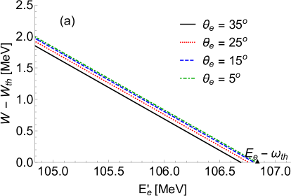
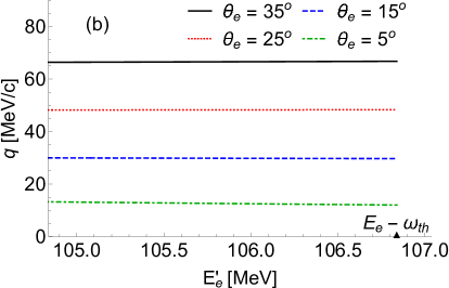
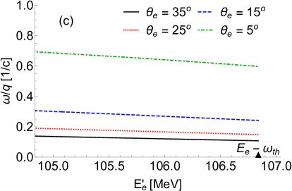
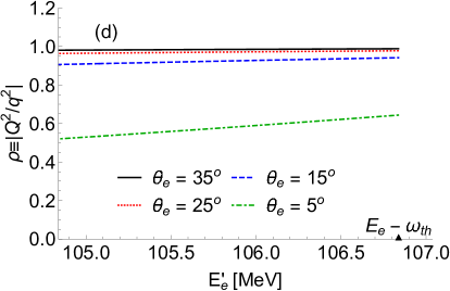
Figure 6: The dependences of the invariant mass above threshold $W-W_{th}$ (a), of the transferred three-momentum $q$ (b), of the ratio of the transferred energy to the transferred three-momentum $\omega/q$ (c), and of the virtuality of the exchanged photon $\rho\equiv|Q^{2}/q^{2}|$ (d), on the scattered electron energy $E^{\prime}_{e}$ for kinematics corresponding to within 2 MeV above threshold.

Figure 7: Leading-order coefficients $a^{\prime}_{E1}$ and $a^{\prime}_{E2}$ as functions of electron scattering angle $\theta_{e}$ at a beam energy $E_{e}$ of 114 MeV.

Given these choices of kinematics in Fig. 7 we then present the leading-order E1 and E2 coefficients, $a^{\prime}_{E1}$ and $a^{\prime}_{E2}$, as functions of $\theta_{e}$ for two values of the $\alpha$-particle $c.m.$ kinetic energy $E_{\alpha}^{c.m.}$, 0.7 and 1.7 MeV (one should remember that these coefficients are constants as functions of $q$ but still depend on $\omega$). One sees that the values of both leading-order coefficients decrease over almost two orders of magnitude when $E_{\alpha}^{c.m.}$ changes from 1.7 to 0.7 MeV, reflecting the steep falloff of the cross section when approaching threshold.

Note that, in the case of the radiative capture reaction, $E_{\alpha}^{c.m.}$ denotes the kinetic energy in the center-of-mass frame of the relative motion of the $\alpha$ and ¹²C pair in the incident channel and can be expressed as $E_{\alpha}^{Lab}M_{{}^{12}C}/(M_{\alpha}+M_{{}^{12}C})$, where $E_{\alpha}^{Lab}$ is the $\alpha$-particle kinetic energy in the laboratory frame. For the electrodisintegration of ¹⁶O, $E_{\alpha}^{c.m.}$ is the difference between the invariant mass $W$ and its value $W_{th}$ at threshold.

Finally, from the continuity equation and in the long wavelength limit $(q\ll q_{0})$ we know how to relate electric $a^{\prime}_{EJ}$ and Coulomb $a^{\prime}_{CJ}$ coefficients (Eq. (59)):

$$a^{\prime}_{CJ}=-\sqrt{\frac{J}{J+1}}a^{\prime}_{EJ}.$$ (64)

V.2 Next-to-leading Order $q$-dependences

Presently we have no information concerning the next-to-leading order contributions in our general parametrization of the multipoles, $b^{\prime}_{CJ,EJ}(q)$ with $J=1,2$. These are independent functions of $q$, i.e., cannot be related via current conservation as can the leading-order contributions. It should be remembered that, at this higher order in $q$, even the way real-$\gamma$ processes are traditionally treated is an approximation, since the electric multipole matrix elements are typically computed as Coulomb matrix elements using the current conservation assumption. Since $\omega/q_{0}=E_{\gamma}/q_{0}$ is not zero, but is small, one is actually making an assumption when following this procedure. In the virtual-$\gamma$ case that occurs with electron scattering the expansion is via higher-order contributions in $q/q_{0}$, and, since $q$ can take on any value where the virtual photon is spacelike, $q>\omega$, as stated earlier, one now has a different situation where when $q\ll q_{0}$ these NLO terms are likely safely negligible; however, if $q$ is allowed to become too large compared with the scale $q_{0}$, then the form taken by these NLO functions may not be simple.

Accordingly, we now make the basic assumption involved in our parametrization of the $C1/E1$ and $C2/E2$ multipoles, namely, we shall assume that the general functions of $q$, $b^{\prime}_{CJ,EJ}(q)$, are in fact constants. When measurements are made these constants will be determined experimentally using the $q$-dependences inherent in the semi-inclusive cross sections. And, with fine enough measurements, one may look for evidence of $q$-dependences that involve even higher powers of $(q/q_{0})^{2}$ to validate the truncations of the expansions.

This strategy is what can be followed when making measurements of the semi-inclusive electrodisintegration cross section as a function of both $q$ and $\omega$. For the present, lacking such measurements, our approach is to make “reasonable” assumptions for these NLO coefficients. Since the multipole matrix elements were parameterized to reflect the nature of spherical Bessel functions, it is reasonable to expect that they are of order unity and accordingly the simplest approximation at present is to assume that $|b^{\prime}_{CJ,EJ}|\approx 1$ for $J=1,2$, and thus the $C1/E1$ and $C2/E2$ multipole matrix elements will be parametrized as

$$t_{CJ}(q) \approx-\sqrt{\frac{J}{J+1}}\bigg{(}\frac{q}{q_{0}}\bigg{)}^{J}a^{\prime}_{EJ}\Bigg{[}1\pm\bigg{(}\frac{q}{q_{0}}\bigg{)}^{2}\Bigg{]}e^{-(q/q_{0})^{2}};$$

$$t_{EJ}(q) \approx\bigg{(}\frac{\omega}{q}\bigg{)}\bigg{(}\frac{q}{q_{0}}\bigg{)}^{J}a^{\prime}_{EJ}\Bigg{[}1\pm\bigg{(}\frac{q}{q_{0}}\bigg{)}^{2}\Bigg{]}e^{-(q/q_{0})^{2}}.$$ (65)

A special case involves the monopole Coulomb matrix element $t_{C0}$: there the leading dependence, which from above would appear to be $(q/q_{0})^{J}$ with $J=0$, cannot occur due to the orthogonality of the initial and final nuclear wave functions and in fact the leading behavior of $t_{C0}(q)$ at low-$q$ is proportional to $(q/q_{0})^{2}$. Again, there are no experimental data which would fix the value of the product $c^{\prime}_{C0}\equiv a^{\prime}_{C0}\cdot b^{\prime}_{C0}$. Therefore, in our feasibility study we investigated the contribution of the $t_{C0}$ to the rate of the ¹⁶O$(e,e^{\prime}\alpha)^{12}$C reaction by setting the $|b^{\prime}_{C0}|=1$ and replacing $a^{\prime}_{C0}$ first with $a^{\prime}_{E2}$, denoted Case A, and then with $0.5\cdot a^{\prime}_{E2}$, denoted Case B. In general, when dealing with experimental data from electrodisintegration of ¹⁶O, $c^{\prime}_{C0}$ needs to be handled as a fit parameter, as with the coefficients $b^{\prime}_{CJ,EJ}$ for $J=1,2$ discussed above. As noted above, we do not know the sign of the $C0$ multipole (i.e., with respect to the other multipoles) and so could have either choice of sign for all interferences between $C0$ and the other multipoles (see below). When presenting results in the following, for the sake of simplicity we have usually chosen the sign to be positive, although both sign choices have been investigated. The detailed angular distributions that result from changing the sign of the $C0$ multipole are found to be comparable but clearly different and accordingly the sign can be determined from the data, as was the case for the $E1/E2$ interference contribution in photodisintegration (see above).

In Figs. 8 ((a) and (b)) we show the semi-inclusive electrodisintegration cross section as a function of $\theta_{\alpha}^{c.m.}$ for two values of $E_{\alpha}^{c.m.}$, at a beam energy $E_{e}$ of 114 MeV and an electron scattering angle $\theta_{e}$ of 15^∘. In each case there are 16 curves corresponding to the two sign choices for each of the next-to-leading order coefficients. Clearly, for the selected kinematics these higher-order effects are quite small, typically less that 6.4%. We again stress that this is not the limiting factor in making such measurements, since, in any actual experiment, the slight extra dependence on $q$ will be determined by varying the kinematics. Having found that the next-to-leading order effects are small, for simplicity henceforth we make the choice $b^{\prime}_{CJ,EJ}=+1$ for $J=1,2$, and, given this choice, Fig. 9 then shows the $\theta_{e}$ dependence of the electric $t_{EJ}$ and Coulomb $|t_{CJ}|$ multipole matrix elements for the selected kinematics.

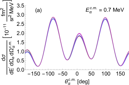
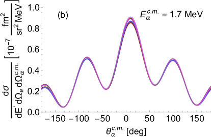
Figure 8: The semi-inclusive electrodisintegration differential cross section as a function of $\theta_{\alpha}^{c.m.}$ at a beam energy $E_{e}$ of 114 MeV and an electron scattering angle $\theta_{e}$ of 15^∘, for $E_{\alpha}^{c.m.}=$ 0.7 MeV (a) and $E_{\alpha}^{c.m.}=$ 1.7 MeV (b). There are 16 curves on each plot corresponding to “$+$” and “$-$” sign choices for each of the four next-to-leading order coefficients $b^{\prime}_{C1}$, $b^{\prime}_{C2}$, $b^{\prime}_{E1}$ and $b^{\prime}_{E2}$. The difference introduced by the change of the sign is so small that the most of the lines are overlapping. At each of the local maxima, it is possible to distinguish two groups of lines which correspond to $+b^{\prime}_{C2}$ and $-b^{\prime}_{C2}$ contributions. Here all interferences involving the $C0$ multipole have been taken to have a plus sign together with the choices of phase differences discussed in the text. Alternatively, all such inteferences could enter with a minus sign.

Figure 9: Electric ($t_{E1}$, $t_{E2}$) and Coulomb ($|t_{C1}|$, $|t_{C2}|)$ multipole matrix elements as functions of the electron scattering angle $\theta_{e}$ at a beam energy $E_{e}$ of 114 MeV.

Finally, we note that in the region of interest $0.7\leq E_{\alpha}^{c.m.}\leq 1.7$ MeV, the elastic phase shifts of the $s$-, $p$- and $d$-waves are almost equal to zero Plaga et al. (1987); Tischhauser et al. (2009) and therefore we neglected them in our calculation of the rate. The only contribution to the phase shift then comes from the Coulomb field, which is equal to the difference of the Coulomb phase shift $\sigma_{l}=\arg\Gamma(1+l+i\eta)$ of partial wave $l$ and the phase shift of the Coulomb monopole $\sigma_{0}=\arg\Gamma(1+i\eta)$ Lane and Thomas (1958):

$$\omega_{l}\equiv\sigma_{l}-\sigma_{0}=\sum_{n=1}^{l}\arctan\frac{\eta}{l}.$$ (66)

We see that the last term in $\phi_{12}$, Eq. (V.1), follows from the general expression, Eq. (66). At the end, we will assume that the phase-shift differences that occur in the electrodisintegration response functions written above, $\delta_{Cl}-\delta_{C0}$ and $\delta_{El}-\delta_{E0}$, are both equal to $\omega_{l}$ for the corresponding partial wave $l$.

Having chosen to use these for the phase-shift differences, as noted above, we must allow for either plus or minus signs to enter for the interferences between the various mutipoles. For the $E1$ and $E2$ cases we follow the lead from photodisintegration and choose the relative sign to be positive. The low-$q$ relationships between $CJ$ and $EJ$ multipoles then fix the signs of the $C1$ and $C2$ multipoles relative to the $E1$ and hence $E2$ multipoles. However, we do not have any information concerning the relative sign of the $C0$ multipole compared with the $C1$, $C2$, $E1$ and $E2$ multipoles. Hence, all terms involving interference with the $C0$ multipole could occur with either sign. During the rest of what is presented in this study usually we arbitrarily choose the sign to be positive, although we have examined what happens when the opposite sign choice is made: the detailed angular distributions change, although are roughly of similar sizes. When measurements are made the appropriate sign choice should be clear following what was done in studies of photodisintegration.

V.3 Electrodisintegration Cross Section Predictions

Having specified the model, we employ this to make projections of the electrodisintegration cross sections in the low-$\omega$ and low-$q$ region and to explore these projections for a range of kinematics, and, in the following section, to provide estimates for the uncertainties that might be expected in practical experiments in extrapolating towards the real-$\gamma$ line and towards threshold. These estimates will then be used to make projections for the desired astrophysical S-factors.

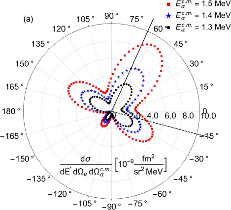
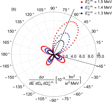
Figure 10: Angular distribution of the ¹⁶O$(e,e^{\prime}\alpha)^{12}$C differential cross section for beam energy of $E_{e}=114$ MeV, electron scattering angle $\theta_{e}=15^{\circ}$ and $\alpha$-particle $c.m.$ kinetic energies $E_{\alpha}^{c.m.}=$ 1.3, 1.4 and 1.5 MeV. The electron beam lies on a ray from 180^∘ to 0^∘, the direction of the scattered electron is represented by a dashed line, and the direction of the virtual photon by a solid line. The results were calculated as a function of $\alpha$-particle $c.m.$ production angle $\theta^{c.m.}_{\alpha}$, but plotted with respect to the direction that the virtual photon has in the laboratory system. Figure (a) shows $t_{C0}$ Case A and (b) Case B.

Figure 10 shows polar plots of the differential cross section for ¹⁶O electrodisintegration as a function of the $\alpha$-particle $c.m.$ production angle $\theta^{c.m.}_{\alpha}$ with respect to the direction of the virtual photon for A (a) and B (b) cases for the choice of $t_{C0}$ discussed above. A very rapid fall-off of the differential cross section can be observed as the $c.m.$ kinetic energy of the $\alpha$-particle decreases. By comparing the (a) and (b) panels in the figure, we see that the choice of the $C0$ coefficient influences to some extent the shape of the differential cross section around the virtual photon direction and its contribution is more important around $\pm 90^{\circ}$ with respect to the virtual photon direction (see later discussion of what impact the monopole contributions have on the extraction of the astrophysical S-factors).

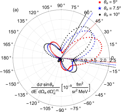
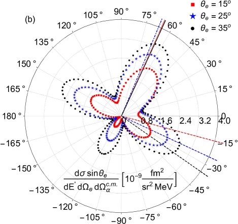
Figure 11: Angular distribution of the ¹⁶O$(e,e^{\prime}\alpha)^{12}$C differential cross section multiplied by $\sin\theta_{e}$ for beam energy of $E_{e}=114$ MeV, $E_{\alpha}^{c.m.}=$ 1.5 MeV, for different electron scattering angles $\theta_{e}=5^{\circ},7.5^{\circ},10^{\circ}({\rm a});15^{\circ},25^{\circ},35^{\circ}({\rm b})$. The electron beam lies on a ray from 180^∘ to 0^∘, the directions of the scattered electrons are represented by dashed lines, and the other type of lines on the positive angle side represents the direction of the virtual photon in the laboratory system.

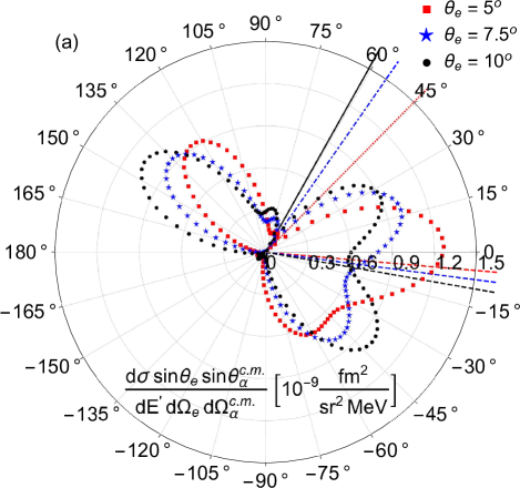
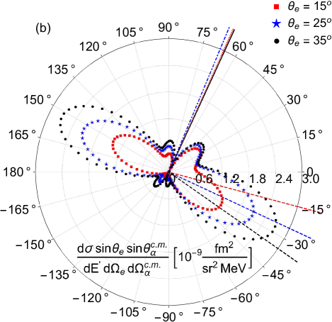
Figure 12: Angular distribution of the ¹⁶O$(e,e^{\prime}\alpha)^{12}$C differential cross section multiplied by $\sin\theta_{e}\cdot\sin\theta_{\alpha}^{c.m.}$ for beam energy of $E_{e}=114$ MeV, $E_{\alpha}^{c.m.}=$ 1.5 MeV, for different electron scattering angles $\theta_{e}=5^{\circ},7.5^{\circ},10^{\circ}({\rm a});15^{\circ},25^{\circ},35^{\circ}({\rm b})$. The electron beam lies on a ray from 180^∘ to 0^∘, the directions of the scattered electrons are represented by dashed lines, and the other type of lines on the positive angle side represents the direction of the virtual photon in the laboratory system.

Figure 11 shows the product of the differential cross section and the electron’s solid angle factor $\sin\theta_{e}$ as a function of $\alpha$ production angle $\theta_{\alpha}^{c.m.}$ for several values of electron scattering angle $\theta_{e}$. The plots suggest that there is no advantage to reaching very low values of $\theta_{e}$, since the product saturates and only increases in magnitude when increasing the electron scattering angle $\theta_{e}$. The increase in magnitude comes from the response functions – at fixed beam energy $E_{e}$ larger $\theta_{e}$ means larger $q$, that is larger values of the response functions. In addition, one needs to keep in mind that a finite sized collimator in a typical electron spectrometer accepts larger angular phase space ($\sin\theta_{e}d\theta_{e}d\phi_{e}$) at smaller electron scattering angle $\theta_{e}$. Later, we will make clear that these two competing effects, for specific experimental conditions, influence the final coincidence rate and, consequently, the statistical uncertainty.

The polar plot of the product of the differential cross section and the solid angle factor $\sin\theta_{e}\sin\theta_{\alpha}^{c.m.}$, shown in Fig. 12, indicates the values of $\theta_{\alpha}^{c.m.}$ for which we can expect the maximum rate of $\alpha$-particle production. For $\theta_{e}\geq$ 15^∘ the maximum rate is around $\pm$90^∘ with respect to the direction of the virtual photon. At energies ($E_{\alpha}^{Lab}\geq 2$ MeV) this can be a good guide to where to place an $\alpha$-particle detector, but at lower energies the placement of the $\alpha$-particle detector will be governed by the minimization of the energy loss and the angular spread of the $\alpha$-particles when traveling through the target material.

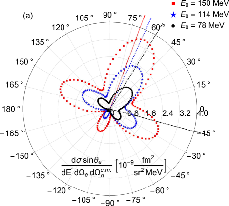
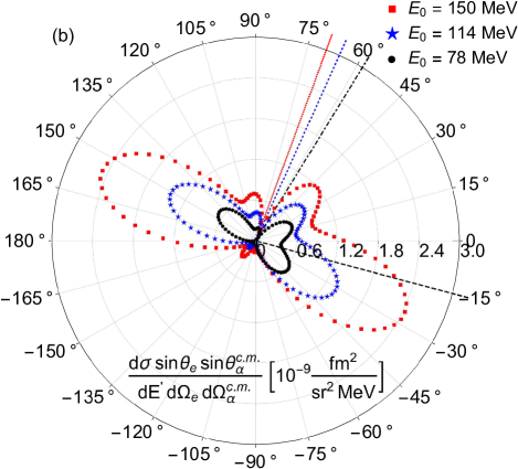
Figure 13: Angular distribution of the ¹⁶O$(e,e^{\prime}\alpha)^{12}$C differential cross section multiplied by $\sin\theta_{e}$ (a) and $\sin\theta_{e}\cdot\sin\theta_{\alpha}^{c.m.}$ (b) for beam energies of $E_{e}=$ 78, 114 and 150 MeV, $E_{\alpha}^{c.m.}=$ 1.5 MeV and electron scattering angle of $\theta_{e}=15^{\circ}$. The electron beam lies on a ray from 180^∘ to 0^∘, the directions of the scattered electrons are represented by dashed lines, and the other type of lines on the positive angle side represents the direction of the virtual photon in the laboratory system.

Figure 13 shows the product of the differential cross section and the solid angle factors $\sin\theta_{e}$ and $\sin\theta_{e}\sin\theta_{\alpha}^{c.m.}$, and illustrates that at fixed electron scattering angle $\theta_{e}$ one can increase the magnitude of the product by increasing the electron beam energy $E_{e}$.

VI Consideration of an Experiment to Measure the ¹⁶O$({\bf e},{\bf e}^{\bf\prime}{\boldsymbol{\alpha}})^{\bf 12}$C Reaction in the Astrophysically Interesting Region

Alpha-cluster knockout in the ¹⁶O(e,e${}^{\prime}\alpha)^{12}$C reaction has been previously studied Meyer et al. (2001) at 615 and 639 MeV incident electron energy. The shape of the measured missing-momentum distribution is reasonably well described by shell-model and cluster-model calculations, but the theoretical curves over-predict the data by a factor of three to four. However, at present, there exists no dedicated set-up for measuring the electrodisintegration of ¹⁶O at lower energies with the astrophysical goals above in mind. Assuming the availability of high intensity energy-recovery linacs (ERLs) in the near future Hug et al. (2017); Hoffstaetter et al. (2017), we here develop a conceptual experiment based on these new, advanced accelerator technologies. In doing so, there are nevertheless practical constraints on what is likely to be possible, and these are discussed below.

VI.1 Experimental Considerations

VI.1.1 Electron Detection

The detector system suitable for measuring the four-momentum of the scattered electron is a high precision, focusing magnetic spectrometer, equipped with focal plane detectors, capable of achieving a momentum resolution $\Delta p_{e}/p_{e}$ better than $\leq 10^{-4}$ and an in-plane scattering angle resolution $\Delta\theta_{e}$ better than $\leq 0.5^{\circ}$. Spectrometers of this type are standard in electron scattering nuclear research, but they differ in angular and momentum acceptance ranges, and in the type of focal plane detector systems used.

VI.1.2 Isotopic and Chemical Contamination

When dealing with the photodisintegration of ¹⁶O into an $\alpha$-particle and ¹²C one needs to take into account a large background coming from $\alpha$-particles produced on ¹⁷O and ¹⁸O. The average isotopic abundances of the oxygen isotopes are 99.7570% for ¹⁶O, 0.03835% for ¹⁷O and 0.2045% for ¹⁸O Meija et al. (2016). The cross sections for photodisintegration of ¹⁷O and ¹⁸O into an $\alpha$-particle and corresponding carbon isotope are several orders of magnitude larger than for the case of photodisintegration of ¹⁶O; see Fig. 14(a). Further, there is always some finite amount of nitrogen present in the oxygen gas (depending on the vendor usually 5 ppmv or less). This will give rise to protons from the photodisintegration reaction ¹⁴N$(\gamma,p)^{13}$C and also contribute to the background. Even if one depletes the ¹⁷O and ¹⁸O by a factor of 1000, and normalizes the cross sections accordingly as shown in the (b) panel of Fig. 14, in the region of interest ($E_{\gamma}=E^{c.m.}_{\alpha}+$ 7.162 MeV) $E_{\gamma}\leq 8.5$ MeV, photodisintegration of ¹⁷O significantly contributes to the background and the contributions of ¹⁸O and ¹⁴N are comparable or at some energies even larger. The same problem can also be expected in the case of electrodisintegration.

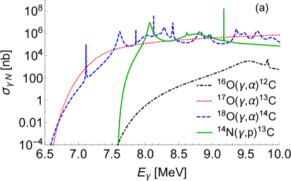
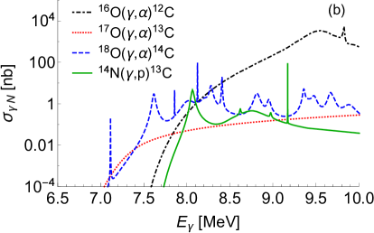
Figure 14: (a) the theoretical photo-nuclear cross section $\sigma_{\gamma N}$ as a function of the gamma energy $E_{\gamma}$ for the signal reaction ¹⁶O$(\gamma,\alpha)^{12}$C, and background reactions ¹⁷O$(\gamma,\alpha)^{13}$C, ¹⁸O$(\gamma,\alpha)^{14}$C and ¹⁴N$(\gamma,p)^{13}$C, from Pho . The same curves are shown on (b), but now the cross sections of the oxygen isotopes were normalized under the assumption that the natural abundances of ¹⁷O and ¹⁸O were depleted by a factor of 1000, and that oxygen gas is contaminated with 5 ppmv of ¹⁴N.

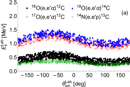
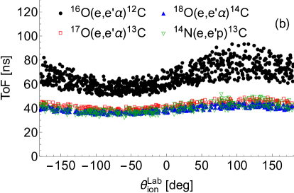
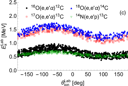
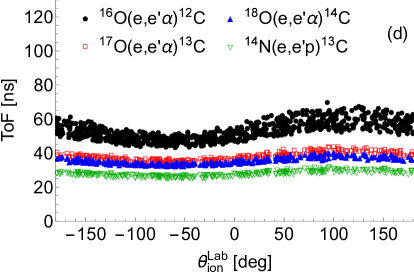
Figure 15: Energy-loss corrected kinetic energy $E_{k}^{Lab}$ and time-of-flight ToF as functions of laboratory ion production angle $\theta^{Lab}_{ion}$ assuming that the ions were produced by electrons involved in the electrodisintegration of ¹⁶O, at $E_{e}=$ 114 MeV and $\theta_{e}=$ 15^∘: (a) and (b) cut on $0.7\leq E_{\alpha}^{c.m.}\leq 0.8$ MeV, (c) and (d) cut on $1.0\leq E_{\alpha}^{c.m.}\leq 1.1$ MeV.

The modern photodisintegration experiments, DiGiovine et al. (2015); Ugalde et al. (2013) and Gai et al. (2010), address these isotopic and chemical contamination issues. Here, we investigate how the background problems can be mitigated in an electrodisintegration experiment with a gas jet target.

In the presented study, SRIM-2013 simulation software Ziegler et al. (2010); SRI was used for calculation of the average energy loss of the $\alpha$-particle or proton at a given kinetic energy in a 2 mm wide ¹⁶O gas jet having a density of 6.65$\times$10^-4 g/cm³. The full electrodisintegration kinematics calculation was performed for oxygen isotopes and ¹⁴N target nuclei, and the data were sorted by selecting the electrons having momenta capable of producing $\alpha$-particles on ¹⁶O in a given $E_{\alpha}^{c.m.}$-range. The kinetic energy of selected $\alpha$-particles and protons was corrected for the energy loss assuming that these particles are created at different positions inside the gas jet. The maximum correction was applied when the particle is created at the edge of the jet and needs to travel through the full extension of the gas jet. In this way, the corrected kinetic energies where converted to time-of-flight (ToF), assuming a flight path of 30 cm between the gas jet and the ion detectors. Figure 15 shows the energy-loss corrected kinetic energies and ToF of the $\alpha$-particles and protons for two $E_{\alpha}^{c.m.}$-ranges. In both cases, we see that the kinetic energy can be used to distinguish the signal from the background $\alpha$-particles. However, to distinguish between protons and $\alpha$-particles from ¹⁶O, the ToF observable is the most effective. It allows a clear background identification and removal from the collected events for all $E_{\alpha}^{c.m.}$ of interest. Furthermore, it is easier to determine the final state of low-energy ions by measuring the ToF and not their kinetic energy $-$ this method is very well known in experimental nuclear physics. Most importantly, such detectors can be designed to be electron blind.

Very close to the reaction threshold one has to deal with $\alpha$-particles having very small kinetic energies, i.e., so small that the target material itself can smear their angular resolution significantly. To quantify the angular smearing by the target material, we used data obtained from a SRIM-2013 simulation to calculate the standard deviation of the $\alpha$-production angle $\Delta\theta^{Lab}_{\alpha}$ as a function of the $\alpha$-particle kinetic energy $E^{Lab}_{\alpha}$; see Fig. 16. At kinetic energy of $E^{Lab}_{\alpha}=$ 0.7 MeV, the standard deviation of the $\alpha$-production angle is already equal to $\Delta\theta^{Lab}_{\alpha}=$ 2.1^∘ and, with deceasing $E^{Lab}_{\alpha}$, the $\Delta\theta^{Lab}_{\alpha}$ starts to increase even faster.

Figure 16: Standard deviation of the $\alpha$-production angle $\Delta\theta^{Lab}_{\alpha}$ as a function of $\alpha$-particle kinetic energy $E^{Lab}_{\alpha}$ for an $\alpha$-particle passing through a 2 mm wide ¹⁶O gas jet with a density of 6.65$\times$10^-4 g/cm³.

Since the circular profile of the jet can be easily changed to a different one, like demonstrated in Köhler et al. (2013). For the fixed luminosity, the problem of the multiple scattering inside the jet can be minimized by extending the jet in the direction of the beam. But in this case, the electron spectrometer will need to have good spatial resolution to be able to reconstruct the position of the vertex along the extended gas jet. Another option, to partially solve this problem, is to make use of the virtual photon properties: at fixed $\omega$ one can independently dial the value of the transferred 3-momentum $q$. Figure 17 shows examples of angular distributions of the $\alpha$-particle kinetic energy for fixed $\omega$ but for two different values of $q$. For larger-$q$, around the direction of the virtual photon ($\sim-$67^∘), the kinetic energy of the $\alpha$ particles is larger compared with the lower-$q$ case. In the opposite direction the larger-$q$ $E^{Lab}_{\alpha}$ is decreased. Ultimately, the measurement close to threshold will need to be performed at an optimized value of $q$, with a gas jet having an optimized density and shape.

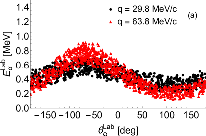
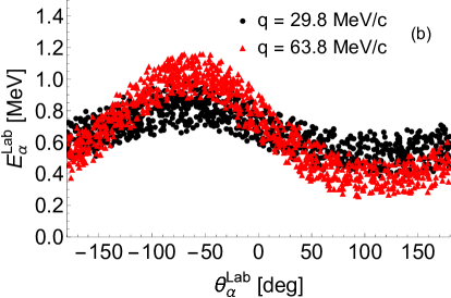
Figure 17: Energy-loss corrected kinetic energy of $\alpha$-particles $E_{\alpha}^{Lab}$ as functions of laboratory $\alpha$ production angle $\theta^{Lab}_{\alpha}$ for two values of transferred 3-momentum of the virtual photon $q$. The (a) panel shows $\alpha$-particles in the range of $0.7\leq E_{\alpha}^{c.m.}\leq 0.8$ MeV, and in the range of $1.0\leq E_{\alpha}^{c.m.}\leq 1.1$ MeV for the (b) panel.

VI.1.3 Alpha-particle Detection

The $\alpha$-particle detector system has to be able to cover the maximum possible solid angle around the beam-target interaction. Further, the detectors have to be blind to electrons, positrons and $\gamma$-rays, due to high rates from elastic, inelastic, and Møller electrons, gammas from radiative processes, and positrons and electrons from radiative pair production. In the region of interest ($0.7\leq E_{\alpha}^{c.m.}\leq 1.7$ MeV) it is straightforward to measure the time-of-light of the $\alpha$-particle to obtain its energy. Thus, these detectors should have a good timing resolution.

Measuring the time-of-light has a crucial advantage since it can be used for ion identification purposes, as well as for distinguishing the $\alpha$-particles coming from different oxygen isotopes.

We have given some consideration to the choice of $\alpha$-particle detector, which is required to detect ions with kinetic energies of about 1 MeV. At 1 MeV kinetic energy, the range in silicon is about 1 mg/cm². Silicon has a density of 2.33 g cm^-2 and so this corresponds to a thickness of 4.3 microns. The count rate for the $(e,e^{\prime}\alpha)$ process is low, $\approx 1-10$ Hz. It is required:

• to measure the total energy of the $\alpha$ to about $\approx\pm 10\%$

• to distinguish between protons, $\alpha$-particles and ¹²C

• to measure the position to $\sim$mm and the timing to a few nsec

• that the ion detection system be blind to scattered electrons and photons.

There are a several different detector possibilities:

• Silicon detector Kordyasz et al. (2015)
  Silicon detectors have a high position resolution in tracking charged particles but are expensive and require cooling to reduce leakage currents. They also suffer degradation over time from radiation; however, by cooling them to low temperatures, this effect can be significantly reversed.

• Micro-channel-plate electron (MCP) detector Friedman et al. (1988)
  A micro-channel plate is a slab made from highly resistive material of typically 2 mm thickness with a regular array of tiny tubes or slots (microchannels) leading from one face to the opposite, densely distributed over the whole surface. The microchannels are typically approximately 10 microns in diameter (6 micron in high resolution MCPs) and spaced apart by approximately 15 microns; they are parallel to each other and often enter the plate at a small angle to the surface ($\approx 8^{\circ}$ from normal).

  The gain of an MCP is very noisy, meaning that two identical particles detected in succession will often produce wildly different signal magnitudes. The temporal jitter resulting from the peak height variation can be removed using a constant fraction discriminator. Employed in this way, MCPs are capable of measuring particle arrival times with very high resolution, making them an ideal detector for mass spectrometers.

• Parallel-plate avalanche counter (PPAC)
  The PPAC detector consists of two parallel thin electrode films separated by 3–4 mm and is filled with 3–50 Torr of gases such as isobutane (C₄H${}_{1}0$) or perfluoropropane (C₃F₈). When a voltage gradient corresponding to a few hundreds of volts per millimeter is applied between the anodes and cathodes, ionized electrons from incident heavy ions immediately cause an electron avalanche. Because there is no time delay before the avalanche occurs and the electrons move at high mobile velocity (mobility), the resulting signals have good timing properties, with rise and fall times of a few nanoseconds, as compared with other types.

  A PPAC detector has been developed at RIKEN RIBF in Japan Kumagai et al. (2013) that has a sensitive area of 240 mm $\times$ 150 mm, and the position information is obtained by a delay-line readout method. Being called a double PPAC, it is composed of two full PPACs, each measuring the particle locus in two dimensions. High detection efficiency has been made possible by the twofold measurement using the double PPAC detector. The sensitivity uniformity is also found to be excellent. The root-mean-square position resolution is measured to be 0.25 mm using an $\alpha$ source, while the position linearity is as good as $\pm$0.1 mm for the detector size of 240 mm.

• Time Projection Chamber
  A time projection chamber (TPC) is a type of particle detector that uses a combination of electric and magnetic fields together with a sensitive volume of gas or liquid to perform a three-dimensional reconstruction of a particle trajectory or interaction.

  A Micromegas TPC is under development Iguaz et al. (2014) for the detection of low-energy heavy ions. The first prototype consists of a 10 $\times$ 10 $\times$ 10 cm³ gaseous vessel equipped with a field shaping cage and a Micromegas detector. With 1 atm of gas, the energy resolution for 6 MeV $\alpha$-particles is about 10%. The window is 10 $\mu$m of Mylar (polyethylene terephthalate) which has a thickness of 1.4 mg cm^-2.

  The DMTPC detector technology has been developed at MIT Deaconu et al. (2017) to search for dark matter. It consists of a TPC filled with low pressure CF₄ gas. Charged particles incident on the gas are slowed and eventually stopped, leaving a trail of free electrons and ionized molecules. The electrons are drifted by an electric field toward an amplification region. Instead of using MWPC endplates for amplification and event readout, as in the traditional TPC design, the DMTPC amplification region consists of a metal wire mesh separated from a copper anode with a high electric field between them. This creates a more uniform electric field in order to preserve the shape of the original track during amplification. The avalanche of electrons also creates a great deal of scintillation light, which passes through the wire mesh. Some of this light is collected by a charge-coupled device (CCD) camera located outside the main detector volume. This results in a two dimensional image of the ionization signal of the track as it appeared on the amplification plane. Information about the charged particle, including its direction of motion within the detector, can be reconstructed from the CCD readout. Additional track information is obtained from readout of the charge signal on the anode plane. The largest existing prototype detectors each have a total of 20 liters of CF₄ gas within the drift region, where measurable events can occur. Recoil ¹⁹F and ¹²C nuclei with energies from 20 keV to 200 keV and $\alpha$-particles from an ²⁴¹Am source have been detected in DMTPC Deaconu et al. (2017).

• Low-Pressure Multistep Detector for Very Low Energy Heavy Ions Astabatyan et al. (2012)
  A large-area timing and position-sensitive multistep gaseous detector designed for the detection of very low energy heavy ions has been developed Breskin and Chechik (1984). It consists of a preamplification stage operating as a parallel plate avalanche chamber directly coupled to a multiwire proportional chamber. The multistep avalanche counter (MSC) was tested with $\alpha$-particles, fission fragments and heavy ions. The detector operates at a pressure range of 1-4 Torr isobutane, with very thin ($\sim$ 50 $\mu$g cm^-2) polypropylene window foils. It has a high gain and good time resolution (better than 180 ps fwhm) and a position resolution better than 0.2 mm (fwhm). Its efficiency for low-energy, high-mass ions was tested with ¹⁶⁰Gd ions and found to be 93% down to kinetic energies of 1.3 MeV. In its original design, the MSC does not provide $\Delta$E information. Information concerning the energy loss, in addition to timing and localization, can be obtained by adding an independent wide-gap collection and low-gain element.

We note that:

• A large area, thin, silicon detector with adequate position resolution and with threshold set so that minimum ionizing particles do not trigger, is an attractive option.

• The first stage could be a thin gas detector, e.g., 10 cm length of gas at 5 Torr. For isobutane (C₄H₁₀), the thickness is 0.15 mg cm^-2. The energy lost by a 1 MeV $\alpha$-particle in such a detector is of order 0.2 MeV.

• This gas detector must be contained in the vacuum system of the gas target. The detector gas volume can be isolated from the gas jet volume by a thin window, e.g., 50 $\mu$g cm^-2 of polypropylene. The energy loss of the $\alpha$-particle will be small in this window.

• The energy lost by a minimizing particle (stopping power $\sim$2 MeV/(g cm^-2)) will be of order 0.5 keV so the gas detector will be blind to scattered electrons.

• The detailed technical aspects of the gas detector (e.g., charge collection mechanism, amplification, transverse size, gas type, etc.) need to be considered in detail. The gas pressure could be high enough to stop the $\alpha$ or it could be thin enough to have another detector (e.g., thin silicon) behind it. Note that a higher detector gas pressure will require a thicker entrance window. Until the details of the gas detector are specified, it is hard to characterize the energy, position and time resolutions.

• Finally, the possibility to integrate the oxygen gas target and the $\alpha$-detector by using the oxygen gas as the ionizing gas for the detector is worthy of consideration.

Below we continue with the calculation of the ¹⁶O$(e,e^{\prime}\alpha)^{12}$C reaction rate and perform an estimate of the statistical uncertainties by using established parameters of existing cluster gas-jet targets Grieser et al. (2018) and expected performance of electron accelerators (MESA Hug et al. (2017) and CBETA Trbojevic et al. (2017)) under construction. In the rate calculations, we identify and consider the most significant sources of systematic uncertainty. Furthermore, systematic effects due to scattering in the gas jet target can be reduced by extending the profile of the jet and/or by increasing the transferred $q$-value; optimization here needs to be carried out experimentally. Nevertheless, in calculation of the rate, we will use what we have learned in this section and restrict the accepted range of the $\alpha$-production angle $\theta_{\alpha}^{c.m.}$ and the accepted $\alpha$-particle kinetic energy $E_{\alpha}^{Lab}$ to reasonable values.

VI.2 Proposed Experiment Concept

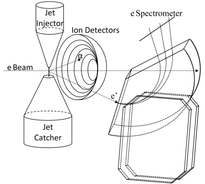
Figure 18: Schematic layout of our proposed ¹⁶O$(e,e^{\prime}\alpha)^{12}$C experiment: ¹⁶O, inside a gas cluster-jet target, is disintegrated by the electron beam into $\alpha$-particles and ¹²C nuclei. The scattered electron is detected in an electron spectrometer and the produced $\alpha$-particle in the ion detectors.

First, having made exploratory projections using our model, we have come to the conclusion that the luminosity should be larger than $10^{35}$ cm^-2s^-1, but that the density of the target oxygen has to be low enough to allow the $\alpha$-particles that exit the target to be detected. A suitable target design here is a windowless oxygen cluster-jet target, like the one described in Grieser et al. (2018). The areal thickness of 2.4$\times$10¹⁸ atoms/cm² was measured for ($\approx$ 2 mm wide) hydrogen jet at a gas temperature of 40 K and gas flow of 40 $l/$min. For our purposes, we will assume one has an oxygen cluster-jet target capable of achieving an areal thickness of 5$\times$10¹⁸ atoms/cm², which for a 2 mm wide jet corresponds to a density of 6.65$\times$10^-4 g/cm³. We also require an electron accelerator which can deliver a beam energy of about 100 MeV and a beam current of at least 10 mA. Two suitable electron accelerators are currently being constructed, namely, MESA, which should deliver a beam current of 10 mA Hug et al. (2017) and CBETA which should be able to go up to 40 mA Trbojevic et al. (2017) for beam energies of 42, 78, 114 and 150 MeV (any energy in between should also be possible). In what follows, we assume a beam current of 40 mA and a jet target as described above, which is equivalent to a luminosity of 1.25$\times$10³⁶ cm^-2s^-1.

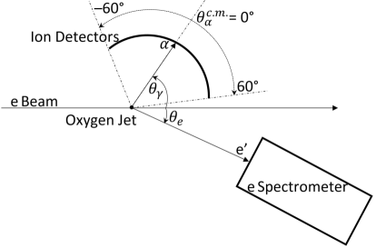
Figure 19: Top-view layout of proposed ¹⁶O$(e,e^{\prime}\alpha)^{12}$C experiment, showing the in-plane angular acceptance of the ion detectors.

To identify events belonging to the ¹⁶O$(e,e^{\prime}\alpha)^{12}$C reaction we need to detect the scattered electron in coincidence with the produced $\alpha$-particle. Fig. 18 shows a schematic layout of a possible experiment.

A high precision magnetic spectrometer is suitable for detection of the scattered electron. For the purpose of defining electrons accepted by the electron spectrometer, we will assume that the spectrometer has an in-plane acceptance of $\pm$2.08^∘ and out-of-plane acceptance of $\pm$4.16^∘; this amounts to a solid angle of 10.5 msr.

Table 1: Summary of experimental parameters for the rate calculation.

Parameters
Oxygen Target	Thickness	5$\times$1018 atoms/cm2
	Density	6.65$\times$10-4 g/cm3
Electron Beam	Current	40 mA
	Energies	78, 114, 150 MeV
Electron arm acceptance	In-plane	$\pm$2.08∘
	Out-of-plane	$\pm$4.16∘
	Solid angle	10.5 msr
$\alpha$-particle arm acceptance	In-plane	60∘
	Out-of-plane	360∘
	Solid angle	3.14 sr
Luminosity		1.25$\times$1036 cm-2s-1
Integrated Luminosity (100 days)		1.08$\times$107 pb-1
Central electron scattering angles		15∘, 25∘, 35∘
$E^{c.m.}_{\alpha}$-range of interest		$0.7\leq E_{\alpha}^{c.m.}\leq 1.7$ MeV

Since we want to obtain S-factors close to the Gamow energy (300 keV), we will need to deal with $\alpha$-particles having very low kinetic energy $E_{\alpha}^{lab}$, (see Fig. 17), where the energy loss in the target and the multiple scattering in the target material play important roles as shown in Fig. 16. In order to select $\alpha$-particles with reasonable energy and angular spread one should either reduce the density of the gas jet or set a cut on the minimum accepted kinetic energy $E_{\alpha}^{Lab}$, i.e., to accept $\alpha$-particles within a certain range around the direction of the virtual photon. We decided to go with the second option and set a cut to accept $\alpha$-particles having a kinetic energy $E_{\alpha}^{Lab}\geq 0.55$ MeV. This cut also imposes a limit on the maximal accepted in-plane scattering angle $\theta^{c.m.}_{\alpha}$, and to cover all settings listed in Table 1 within an equal angular range, only $\alpha$-particles having an in-plane scattering angle $\theta^{c.m.}_{\alpha}$ in the range from 0^∘ to 60^∘ were accepted. For the out-of-plane angle $\phi_{\alpha}$, the full acceptance from 0^∘ to 360^∘ was assumed. Note that by selecting the full range of $\phi_{\alpha}$, the integral of interference response functions $R_{TT}$ and $R_{TL}$ over $\phi_{\alpha}$ will be equal to zero and only longitudinal $R_{L}$ and transverse $R_{T}$ response functions will contribute to the total cross section. Figure 19 shows a top-view layout of the experiment.

Table 2 summarizes the assumptions for the parameters used in the differential cross section (Eq. (21)) used for the calculation of the rate and subsequent statistical uncertainties.

Table 2: Summary of theoretical assumptions for the rate calculation.

Assumptions
$b^{\prime}_{CJ,EJ}$	Value	$\approx 1$ for $J=1,2$
	Sign	”$+$” for $J=1,2$
$c^{\prime}_{C0}\equiv a^{\prime}_{C0}\times b^{\prime}_{C0}$	Value of $b^{\prime}_{C0}$	$\approx 1$
	Value of $a^{\prime}_{C0}$	$=a^{\prime}_{E2}$, Case A
		$=0.5a^{\prime}_{E2}$, Case B
$t_{C0}$	Sign	”$+$”
In $E^{c.m.}_{\alpha}$-region of interest only the Coulomb phase
contributes.

VI.3 Estimation of Event Rates

Since it is difficult to calculate the rate analytically, we have carried out a numerical simulation of the conceptual experiment illustrated in Fig. 18. By using Monte Carlo integration and explicit experimental parameters (see Table 1) and theoretical assumptions (see Table 2), we have estimated the rate of the coincidences per day in the energy range $0.7\leq E_{\alpha}^{c.m.}\leq 1.7$ MeV divided into 100 keV wide bins; see Fig. 20. For $t_{C0}$ Case A the coincidence rate ranged from 73 day^-1 up to 30602 day^-1, and for Case B from 55 day^-1 up to 23123 day^-1. In total, the coincidence rate of $t_{C0}$ Case A is $\approx$32% larger than for Case B.

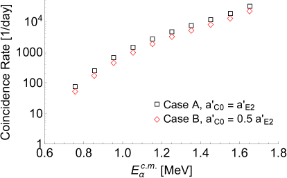
Figure 20: Coincidence rate per day for $t_{C0}$ Cases A and B, for electron beam energy of $E_{e}=$ 114 MeV, central electron scattering angle of $\theta_{e}=$ 15^∘, electron spectrometer acceptance of 10.5 msr, $\alpha$-particle detector acceptance of 3.14 sr and luminosity of 1.25$\times$10³⁶ cm^-2s^-1.

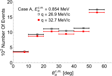
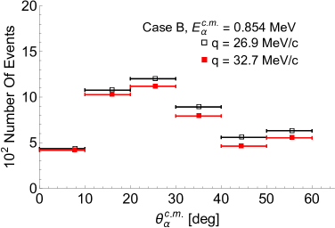
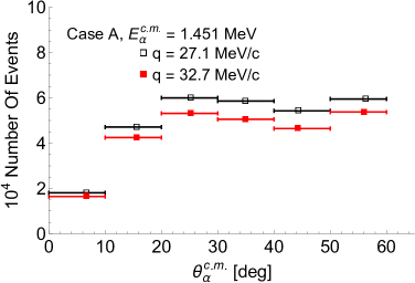
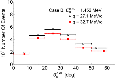
Figure 21: Number of events as a function of $\theta^{c.m.}_{\alpha}$ assuming 100 days of data taking at the luminosity of $2.5\times 10^{36}$ cm^-2s^-1. The left column represents $t_{C0}$ Case A and right one Case B. Horizontal bars denote the width of the $\theta^{c.m.}_{\alpha}$-bin which here is equal to 10^∘. Horizontal placement of the data point within a bin was done according to the procedure recommended in Lafferty and Wyatt (1995). The $q$-bins are 1.91 MeV/c wide and $E_{\alpha}^{c.m.}$-bins 100 keV. For all events inside a particular $q$- and $E_{\alpha}^{c.m.}$-bin, the specified $q$-values represent the average value, and the stated $E_{\alpha}^{c.m.}$-values represent the average of the expected and averaged $E_{\alpha}^{c.m.}$-value.

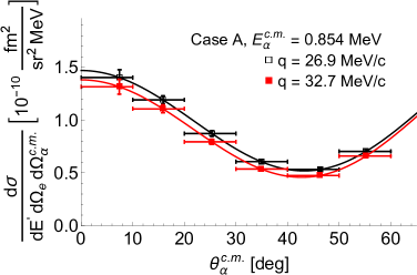
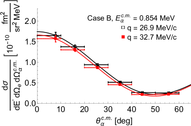
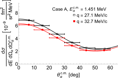
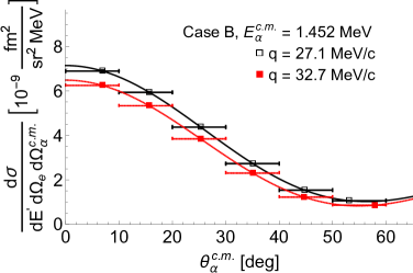
Figure 22: Differential cross section as function of $\theta^{c.m.}_{\alpha}$. The left column represents $t_{C0}$ Cases A and right Case B. Vertical bars correspond to statistical uncertainties assuming 100 days of data taking at the luminosity of $2.5\times 10^{36}$ cm^-2s^-1. The same binning procedure was performed as described in caption of Fig. 21.

In order to mimic the data treatment in a real experiment, the accepted events in the energy range $0.7\leq E_{\alpha}^{c.m.}\leq 1.7$ MeV were placed in 100 keV wide bins, for which, as shown in figure 15, it is possible to identify the $\alpha$-particles from electrodisintegration of ¹⁶O and fully separate them from the background. Additionally, the full range of accepted electron scattering angle $\theta_{e}$ was divided into four bins corresponding to four different $q$-values, and events in each $\theta_{e}$-bin were finally sorted into six $\theta_{\alpha}^{c.m.}$-bins ranging from 0^∘ to 60^∘. An example of the sorting can be seen in Fig. 21. The rate was converted into the number of events collected over 100 days by multiplying it with the integrated luminosity of 1.08$\times$10⁷pb^-1.

The number of events per bin was used to calculate the corresponding statistical uncertainty and this is the quantity for which we performed the above described procedure, since it determines how large an advantage one might have measuring the electrodisintegration of ¹⁶O compared with previous experiments.

VI.4 Estimated Uncertainties in Determination of Astrophysical S-Factors

Now that we have determined the angular distribution of the number of events, we can proceed to predict the astrophysical S-factors, with associated uncertainties. First, the event distribution is converted back into the differential cross section distribution by dividing it with the Monte Carlo integrated phase space covered by each bin and the integrated luminosity, but now including the statistical uncertainties; see Fig. 22.

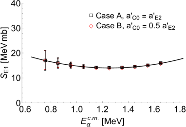
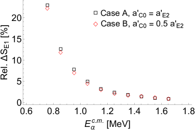
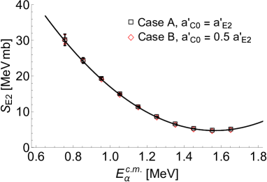
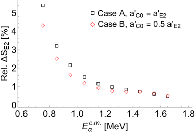
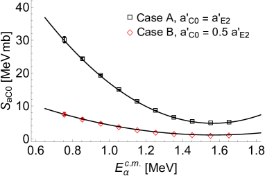
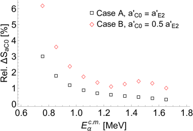
Figure 23: Reconstructed astrophysical $S_{E1}$- and $S_{E2}$-factors, showing their absolute (left column) and relative uncertainties (right column) for $t_{C0}$ Case A and B, $E_{e}=$ 114 MeV and $\theta_{e}=$ 15^∘. $S_{aC0}$ does not have an astrophysical counterpart and it just a conversion of the third fitting parameter into an S-factor and corresponding uncertainty in order to put it in perspective with $S_{E1}$ and $S_{E2}$.

The Levenberg-Marquardt method was used to extract three fitting parameters $a^{{}^{\prime}}_{E1}$, $a^{{}^{\prime}}_{E2}$ and $a^{{}^{\prime}}_{C0}$ (from the Coulomb monopole) from the data, as well as their uncertainties. At given $E_{\alpha}^{c.m.}$-bin we obtained four values for each fitting parameter originating from four $q$-bins, which were combined together by taking the average value of each parameter and by calculating their total uncertainty. The last step is to invert Eq. (V.1) and for each $E_{\alpha}^{c.m.}$-bin calculate the $S_{E1}$- and $S_{E2}$-factors and their uncertainties; see Fig. 23 as an example for $t_{C0}$ Case A and Case B at $E_{e}=$ 114 MeV and $\theta_{e}=$ 15^∘. When we compare $t_{C0}$ Cases A and B, the value of $a^{\prime}_{C0}$ has a minor effect ($\sim$3%) on the uncertainties in $S_{E1}$. For the same comparison, the relative uncertainties in $S_{E2}$ are approximately 25% larger in Case A, but the uncertainties in $S_{aC0}$ in Case B are twice as large as in Case A. The ”bump” in the relative uncertainties of $S_{aC0}$ Case B is caused by fluctuation in $\theta_{\alpha}^{c.m.}$-position of the data point inside the last bin $50^{\circ}<\theta_{\alpha}^{c.m.}<60^{\circ}$.

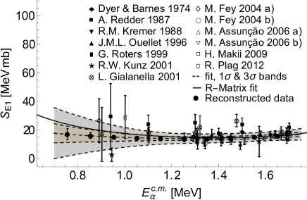
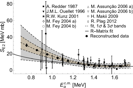
Figure 24: Reconstructed astrophysical $S_{E1}$- and $S_{E2}$-factors with statistical error bars (represented by solid circles) from our calculation for $E_{e}=$ 114 MeV, $\theta_{e}=$ 15^∘, $t_{C0}$ Case A, together with experimental data from Dyer and Barnes (1974); Redder et al. (1987); Kremer et al. (1988); Ouellet et al. (1996); Roters et al. (1999); Kunz et al. (2001); Kunz (2002); Gialanella et al. (2001); Fey (2004); Assunção et al. (2006); Makii et al. (2009); Plag et al. (2012) and Azure2 R-Matrix fit Azuma et al. (2010).

Figure 24 shows one example of the calculated $S_{E1}$- and $S_{E2}$-factors with projected statistical uncertainties for parameters $E_{e}=$ 114 MeV, $\theta_{e}=$ 15^∘ and $t_{C0}$ Case A, as well as data from past experiments. These results are also plotted in terms of relative uncertainties in Fig. 25 to point out a clear advantage of measuring the ¹⁶O$(e,e^{\prime}\alpha)^{12}$C reaction for several $E_{\alpha}^{c.m.}$ energies. Compared with the most accurate measurements from Fey (2004) and Makii et al. (2009), the relative uncertainties in $S_{E1}$ and $S_{E2}$ at a given energy are improved at least by factors of $\times$5.6 and $\times$23.9, respectively.

Figure 25: Relative uncertainties of reconstructed the astrophysical $S_{E1}$- and $S_{E2}$-factors (represented by solid circles) from our calculation for $E_{e}=$ 114 MeV, $\theta_{e}=$ 15^∘, $t_{C0}$ Case A and relative errors from Dyer and Barnes (1974); Redder et al. (1987); Kremer et al. (1988); Ouellet et al. (1996); Roters et al. (1999); Kunz et al. (2001); Kunz (2002); Gialanella et al. (2001); Fey (2004); Assunção et al. (2006); Makii et al. (2009); Plag et al. (2012) experiments. Data points with uncertainties larger then 140% are not shown.

In the following Figs. 27$-$27, we summarize the calculation of the projected relative uncertainties in the $S_{E1}$-, $S_{E2}$- and $S_{aC0}$-factors as functions of the beam energies $E_{e}=$ 78, 114 and 150 MeV and the electron scattering angles $\theta_{e}=$ 15^∘, 25^∘ and 35^∘. Even for values of $E_{e}$, $\theta_{e}$ and $t_{C0}$, which give the worst projected statistical uncertainties, improvements in the relative uncertainties of $S_{E1}$ and $S_{E2}$ at a given energy, compared with previous experimental data from Fey (2004) and Makii et al. (2009), are at least $\times$2.6 and $\times$15.5, respectively.

In general, with increasing electron beam energy $E_{e}$ all uncertainties are reduced. This can be easily understood, because at fixed central electron scattering angle $\theta_{e}$ the accepted angular phase space of the electron is also fixed, but at larger beam energy $E_{e}$ we also get a larger $q$ value, and thus the coincidence rate is larger.

If we vary the central electron scattering angle $\theta_{e}$ at fixed beam energy $E_{e}$, the uncertainty in $S_{E1}$ is smaller at smaller values of angle $\theta_{e}$, which favors the kinematic setting having a larger accepted electron angular phase space, thus having the larger rate for fixed $E_{e}$. The uncertainty in $S_{E2}$ behaves the opposite way, favoring the kinematic setting with larger $q$ value at fixed $E_{e}$.

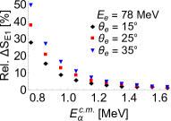
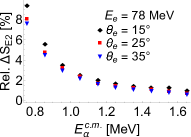
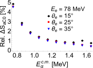
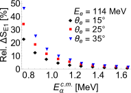
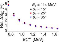
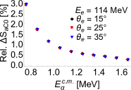
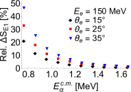
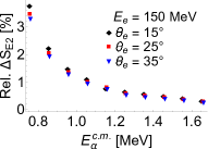
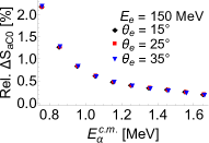
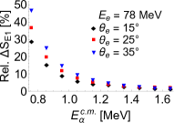
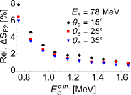
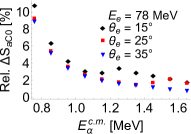
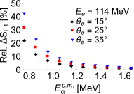
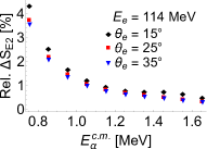
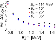
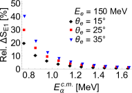
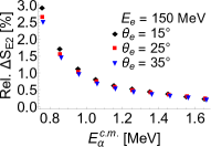
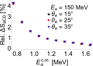
Figure 26: Relative uncertainties of the $S_{E1}$-, $S_{E2}$- and $S_{aC0}$-factors for several values of beam energies $E_{e}$, electron scattering angles $\theta_{e}$ and for $t_{C0}$ Case A. The $S_{aC0}$ does not have an astrophysical counterpart and it just a conversion of the third fitting parameter into an S-factor and corresponding uncertainty in order to put it in a perspective with $S_{E1}$ and $S_{E2}$.

Figure 27: Same as in the caption of Fig. 27, but for $t_{C0}$ Case B.

VI.5 Discussion of Results

The results summarized in Figs. 24$-$25 offer significant potential that the $S$-factors associated with the $E1$ and $E2$ multipoles of the ¹⁶O$(e,e^{\prime}\alpha)^{12}$C reaction at astrophysical energies can be determined with significantly reduced uncertainties. We would like to emphasize important details about the assumptions we have made:

• Although we obtained excellent results in reducing the statistical uncertainties, note that our calculation does not include detailed consideration of systematic uncertainties, which are always present in experimental data. However, we are not aware of any systematic effect that can reduce the large improvement in the determination of the radiative capture reaction with our new approach. At fixed beam energy $E_{e}$ and electron scattering angle $\theta_{e}$, the electron spectrometer detects scattered electrons in a narrow range of electron momenta $E_{e}^{{}^{\prime}}$ and the $\theta_{e}$. Therefore, one can expect that the systematic uncertainty connected with the detection of the electron will not vary significantly over these ranges. As discussed in section VI.1.2, the systematic uncertainties related to the detection of the $\alpha$-particles are very energy dependent. They increase rapidly as the $\alpha$-particle kinetic energy $E_{\alpha}^{Lab}$ decreases; see for example Fig. 16. However, we note that the kinetic energy of the $\alpha$-particle can be controlled by the transferred momentum $q$ and the thickness of the jet-target traversed by the $\alpha$-particle can be reduced by extending the shape of the jet’s profile. This optimization needs further consideration.

• One significant source of systematic uncertainty which needs to be considered is the uncertainty of the electron beam energy $E_{e}$, which is especially important at low $E_{\alpha}^{c.m.}$-values. In a coincidence measurement of the electrodisintegration of ¹⁶O, the kinematics are over-determined. Thus, an attractive method to determine the electron beam energy would be to reconstruct the energy of the electron beam $E_{e}$ for each coincidence $e^{\prime}\alpha$ pair separately.

• The Coulomb and electric multipole matrix elements have only been expanded up to the NLO, see Eq. (50) and (54), and for the corresponding NLO coefficients we assumed $b^{\prime}_{CJ,EJ}\approx 1$. In general these coefficients are functions of $q$ and, when dealing with experimental ¹⁶O$(e,e^{\prime}\alpha)^{12}$C data, their magnitude and $q$-behavior will have to be verified by including them as four additional fitting parameters. If values of $b^{\prime}_{C0,C1,C2,E1,E2}$ are smaller than unity for large range of $q$, truncating the expansion of multipole matrix elements at the NLO term is justified. But, if the values are larger than 1, we may need to include the third-order in the expansion with corresponding coefficients $c^{\prime}_{CJ,EJ}$. Which order in this expansion needs to be included can easily be verified by measuring the rate of electrodisintegration of ¹⁶O at several larger $q$-points.

• The calculations here were focused on the $E_{\alpha}^{c.m.}$-range from 0.7 to 1.7 MeV, but a typical electron spectrometer has at least a momentum acceptance of 10% and for $E_{e}=$ 78 MeV the full available $E_{\alpha}^{c.m.}$-range would be from 0.0 to 6.7 MeV, or for $E_{e}=$ 150 MeV from 0.0 to 13.6 MeV. By choosing the appropriate beam energy, a single ¹⁶O electrodisintegration measurement could cover the $E_{\alpha}^{c.m.}$-range of almost all previous experiments, and crosscheck their results. Furthermore, at higher $\alpha$-energies, multipoles $E3$ and $C3$ could start to significantly contribute to the cross section (although this was not yet observed deBoer et al. (2017)). Because of this we have provided the multipole decomposition of the response functions up to octupole terms in the Appendix A.

• For all choices of the parameters $E_{e}$ and $\theta_{e}$ we obtained a smaller uncertainty for $S_{E2}$ compared to $S_{E1}$. There are two reasons for this result. Firstly, the $C2/E2$ matrix elements which enter in the response functions $R_{L,T,TL,TT}$ differ from $C1/E1$ matrix elements by a factor $q/\omega$. This is the dominant contribution, which does not exist in the case of real photon experiments, since $q/\omega=$ 1. Secondly, a minor contribution comes from the $\theta^{c.m.}_{\alpha}$-distribution of the relevant multipoles. In the $\theta^{c.m.}_{\alpha}$-range from 0^∘ to 60^∘, the magnitudes of the $C2/E2$ $\theta^{c.m.}_{\alpha}$-distributions are larger compared with those of the $C1/E1$. The same behavior can also be observed for the $E1$ and $E2$ multipoles in the case of real-photon experiments; for example this is shown in Fig. 5 in deBoer et al. (2017).

• In section VI.1.2 we have considered the most probable sources of background and demonstrated how to identify the $\alpha$-particles from the electrodisintegration of ¹⁶O. If one takes a closer look at figures 14 and 15, in the same experiment, we can also identify the proton and measure the rate of the ¹⁴N$(e,e^{\prime}p)^{13}$C reaction. Furthermore, the photodisintegration cross section of ¹⁸O is much larger compared with that of ¹⁷O and, with further work, it would also be possible to extract the rate of the ¹⁸O$(e,e^{\prime}\alpha)^{14}$C reaction. Note that with minor modifications, the same formalism presented in this paper for electrodisintegration of ¹⁶O can also be be applied to electrodisintegration of ¹⁸O.

VII Conclusion and outlook

In summary, we have considered in some detail a new approach to determine radiative capture reactions at astrophysical energies. Using detailed balance, we consider the inverse electron-induced disintegration process. Specifically, in this paper we have focused on the ¹⁶O(e,e${}^{\prime}\alpha$)¹²C reaction as a means to determine the astrophysically crucial radiative capture process ¹²C($\alpha,\gamma$)¹⁶O. We have applied a multipole decomposition constrained to fit existing data together with some reasonable theoretical assumptions to extrapolate from the electrodisintegration process to the photodisintegration reaction. We have developed a Monte Carlo simulation of an experiment where an external electron beam is directed on an oxygen gas jet target; the forward scattered electron is detected in a magnetic spectrometer and the coincident, low-energy, recoil $\alpha$-particle is detected in a large acceptance detector centered around the direction of three-momentum transfer. We assume what we believe are reasonable experimental parameters to carry out such an experiment at the upcoming ERLs. With an electron beam of energy 114 MeV and beam current of 40 mA incident on a hydrogen gas target of $5\times 10^{18}$ cm^-2, we estimate that $S_{E1}$- and $S_{E2}$- factors can be determined at $E^{c.m.}_{\alpha}$ = 0.75 MeV to of order $\pm$20% and $\pm$5%, respectively, in 100 days of continuous data taking.

Assuming that the multi-Megawatt ERLs are realized with electron energy of about 100 MeV, a key technical challenge is to realize efficient, large solid-angle, low-energy $\alpha$-particle detection that is blind to the large rate of electromagnetic background. We note that previous work has shown Alarcon et al. (2013) that the electron beam quality of 100 MeV Megawatt ERLs is high, with $\sim$50 $\mu$m 1$\sigma$ spatial size and with minimal halo. To reach high precision, the experiment must be efficient and stable over months of data taking. However, we stress that the initial, key experiment to validate our proposed approach should focus on higher $E^{c.m.}_{\alpha}$ where the coincident electrodisintegration rates are significantly higher than in the astrophysical region and accordingly the running time is a more modest several weeks. Such an experiment should elucidate the multipole structure of the electrodisintegration reaction, whose understanding is essential for extrapolation to the photodisintegration reaction. If our approach is validated experimentally, one can then embark on the more ambitious measurement to determine the S-factors in the astrophysically interesting region at low $\alpha$-particle energies, where the electrodisintegration count rate drops precipitously.

In the present study, we have focused on electrodisintegration of ¹⁶O into the ground states of ⁴He and ¹²C in the low momentum transfer $q$ region near threshold for the reaction. We have provided the bridge to photodisintegration and radiative capture (real-photon) reactions through the limit where the virtual photon involved in electron scattering becomes close to the real-photon line. Measurements of electrodisintegration thereby have the potential to provide a new way to approach the real-$\gamma$ photodisintegration cross sections and hence, through detailed balance, the capture reaction cross section and ultimately the astrophysical S-factors involved in that process. As discussed in the Introduction, obtaining information on these last quantities provides one of the high-priority goals in nuclear astrophysics.

After developing the general formalism for the electrodisintegration reaction ¹⁶O$(e,e^{\prime}\alpha){}^{12}$C following past general treatments of such semi-inclusive reactions, together with some discussion of the photodisintegration reaction ¹⁶O$(\gamma,\alpha){}^{12}$C and radiative capture reaction $\alpha+{}^{12}$C$\rightarrow\gamma+{}^{16}$O, we have proceeded to develop parametrizations for the dynamical content in the problem. Since our focus is the region near threshold for the photo- or electro-disintegration reactions we are assured that the energy of the photon, $E_{\gamma}$, is small. Additionally, we have limited our attention to kinematics where the three-momentum transfer carried by the virtual photon in electrodisintegration, $q$, is also small. Here one needs to state what is meant by “small”. We expect that the nuclear dynamics involved in the reactions occur with a typical nuclear scale $q_{0}\cong 200$ – 250 MeV/c, and accordingly we measure both quantities versus $q_{0}$, taking both ratios $\mu_{1}\equiv E_{\gamma}/q_{0}$ and $\mu_{2}\equiv q/q_{0}$ to be small. This allows us to expect that the lowest multipoles will dominate over higher multipolarity contributions and also to expand each of the small number of remaining multipoles in powers of $\mu_{1,2}$. Ultimately, as we have shown in detail in the body of this work, there are only a few parameters left that determine the dynamical content of the problem in the kinematic region of interest. Such procedures are simply an extension of what is typically done for photodisintegration or radiative capture.

Of course, it would be valuable to have a microscopic model for the reactions of interest here, although this is far from realizable at present. Even relatively crude models might be of some interest as they could help set the scales in the problem. For example, a cluster model in which the ¹²C ground state might be taken to be a cluster of three $\alpha$-particles and the ground state of ¹⁶O might involve four $\alpha$-particles could be pursued. We have not done so in this initial study, but instead have limited our attention to the parametrizations discussed above. When measurements are made of the kinematical dependences on $q$ and the angular distributions of the $\alpha$-particles are determined for each energy above threshold there is ample information to fix all of the parameters involved experimentally.

*

Appendix A Extended Angular Distributions

Following Raskin and Donnelly (1989), the responses in terms of Legendre polynomials up to octupole contributions may be written

$$R_{L} =P_{0}(\cos\theta_{\alpha})\Bigg{(}|t_{C0}|^{2}+|t_{C1}|^{2}+|t_{C2}|^{2}+|t_{C3}|^{2}\Bigg{)}$$

$$+P_{1}(\cos\theta_{\alpha})\Bigg{(}2\sqrt{3}|t_{C0}||t_{C1}|\cos(\delta_{C1}-\delta_{C0})+4\sqrt{\frac{3}{5}}|t_{C1}||t_{C2}|\cos(\delta_{C2}-\delta_{C1})+\frac{18}{\sqrt{35}}|t_{C2}||t_{C3}|\cos(\delta_{C3}-\delta_{C2})\Bigg{)}$$

$$+P_{2}(\cos\theta_{\alpha})\Bigg{(}2|t_{C1}|^{2}+\frac{10}{7}|t_{C2}|^{2}+2\sqrt{5}|t_{C0}||t_{C2}|\cos(\delta_{C2}-\delta_{C0})+6\sqrt{\frac{3}{7}}|t_{C1}||t_{C3}|\cos(\delta_{C3}-\delta_{C1})+\frac{4}{3}|t_{C3}|^{2}\Bigg{)}$$

$$+P_{3}(\cos\theta_{\alpha})\Bigg{(}6\sqrt{\frac{3}{5}}|t_{C1}||t_{C2}|\cos(\delta_{C2}-\delta_{C1})+\frac{8}{3}\sqrt{\frac{7}{5}}|t_{C2}||t_{C3}|\cos(\delta_{C3}-\delta_{C2})+2\sqrt{7}|t_{C0}||t_{C3}|\cos(\delta_{C3}-\delta_{C0})\Bigg{)}$$

$$+P_{4}(\cos\theta_{\alpha})\Bigg{(}\frac{18}{7}|t_{C2}|^{2}+8\sqrt{\frac{3}{7}}|t_{C1}||t_{C3}|\cos(\delta_{C3}-\delta_{C1})+\frac{18}{11}|t_{C3}|^{2}\Bigg{)}$$

$$+P_{5}(\cos\theta_{\alpha})\Bigg{(}\frac{20}{3}\sqrt{\frac{5}{7}}|t_{C2}||t_{C3}|\cos(\delta_{C3}-\delta_{C2})\Bigg{)}$$

$$+P_{6}(\cos\theta_{\alpha})\Bigg{(}\frac{100}{33}|t_{C3}|^{2}\Bigg{)}$$ (67)

$$R_{T} =P_{0}(\cos\theta_{\alpha})\Bigg{(}|t_{E1}|^{2}+|t_{E2}|^{2}+|t_{E3}|^{2}\Bigg{)}$$

$$+P_{1}(\cos\theta_{\alpha})\Bigg{(}\frac{6}{\sqrt{5}}|t_{E1}||t_{E2}|\cos(\delta_{E2}-\delta_{E1})+12\sqrt{\frac{2}{35}}|t_{E2}||t_{E3}|\cos(\delta_{E3}-\delta_{E2})\Bigg{)}$$

$$+P_{2}(\cos\theta_{\alpha})\Bigg{(}-|t_{E1}|^{2}+\frac{5}{7}|t_{E2}|^{2}+6\sqrt{\frac{2}{7}}|t_{E1}||t_{E3}|\cos(\delta_{E3}-\delta_{E1})+|t_{E3}|^{2}\Bigg{)}$$

$$+P_{3}(\cos\theta_{\alpha})\Bigg{(}-\frac{6}{\sqrt{5}}|t_{E1}||t_{E2}|\cos(\delta_{E2}-\delta_{E1})+\frac{2}{3}\sqrt{\frac{14}{5}}|t_{E2}||t_{E3}|\cos(\delta_{E3}-\delta_{E2})\Bigg{)}$$

$$+P_{4}(\cos\theta_{\alpha})\Bigg{(}-\frac{12}{7}|t_{E2}|^{2}-6\sqrt{\frac{2}{7}}|t_{E1}||t_{E3}|\cos(\delta_{E3}-\delta_{E1})+\frac{3}{11}|t_{E3}|^{2}\Bigg{)}$$

$$+P_{5}(\cos\theta_{\alpha})\Bigg{(}-\frac{10}{3}\sqrt{\frac{10}{7}}|t_{E2}||t_{E3}|\cos(\delta_{E3}-\delta_{E2})\Bigg{)}$$

$$+P_{6}(\cos\theta_{\alpha})\Bigg{(}-\frac{25}{11}|t_{E3}|^{2}\Bigg{)}$$ (68)

$$R_{TT} =-R_{T}\cos(2\phi_{\alpha}).$$ (69)

$$R_{TL} =\cos\phi_{\alpha}\Bigg{\{}P^{1}_{1}(\cos\theta_{\alpha})\Bigg{(}2\sqrt{3}|t_{C0}||t_{E1}|\cos(\delta_{E1}-\delta_{C0})-2\sqrt{\frac{3}{5}}|t_{C2}||t_{E1}|\cos(\delta_{C2}-\delta_{E1})$$

$$+\frac{6}{\sqrt{5}}|t_{C1}||t_{E2}|\cos(\delta_{C1}-\delta_{E2})-6\sqrt{\frac{3}{35}}|t_{C3}||t_{E2}|\cos(\delta_{C3}-\delta_{E2})+6\sqrt{\frac{6}{35}}|t_{C2}||t_{E3}|\cos(\delta_{C2}-\delta_{E3})\Bigg{)}$$

$$+P^{1}_{2}(\cos\theta_{\alpha})\Bigg{(}2|t_{C1}||t_{E1}|\cos(\delta_{C1}-\delta_{E1})+2\sqrt{\frac{5}{3}}|t_{C0}||t_{E2}|\cos(\delta_{E2}-\delta_{C0})+\frac{10}{7\sqrt{3}}|t_{C2}||t_{E2}|\cos(\delta_{C2}-\delta_{E2})$$

$$-2\sqrt{\frac{3}{7}}|t_{C3}||t_{E1}|\cos(\delta_{C3}-\delta_{E1})+4\sqrt{\frac{2}{7}}|t_{C1}||t_{E3}|\cos(\delta_{C1}-\delta_{E3})+\frac{2}{3}\sqrt{\frac{2}{3}}|t_{C3}||t_{E3}|\cos(\delta_{C3}-\delta_{E3})\Bigg{)}$$

$$+P^{1}_{3}(\cos\theta_{\alpha})\Bigg{(}2\sqrt{\frac{3}{5}}|t_{C2}||t_{E1}|\cos(\delta_{C2}-\delta_{E1})+\frac{4}{\sqrt{5}}|t_{C1}||t_{E2}|\cos(\delta_{C1}-\delta_{E2})$$

$$+2\sqrt{\frac{7}{6}}|t_{C0}||t_{E3}|\cos(\delta_{E3}-\delta_{C0})+\frac{2}{3}\sqrt{\frac{7}{15}}|t_{C3}||t_{E2}|\cos(\delta_{C3}-\delta_{E2})+2\sqrt{\frac{7}{30}}|t_{C2}||t_{E3}|\cos(\delta_{C2}-\delta_{E3})\Bigg{)}$$

$$+P^{1}_{4}(\cos\theta_{\alpha})\Bigg{(}\frac{6\sqrt{3}}{7}|t_{C2}||t_{E2}|\cos(\delta_{C2}-\delta_{E2})+2\sqrt{\frac{3}{7}}|t_{C3}||t_{E1}|\cos(\delta_{C3}-\delta_{E1})$$

$$+\frac{6}{\sqrt{14}}|t_{C1}||t_{E3}|\cos(\delta_{C1}-\delta_{E3})+\frac{6}{11}\sqrt{\frac{3}{2}}|t_{C3}||t_{E3}|\cos(\delta_{C3}-\delta_{E3})\Bigg{)}$$

$$+P^{1}_{5}(\cos\theta_{\alpha})\Bigg{(}\frac{40}{3}\frac{1}{\sqrt{105}}|t_{C3}||t_{E2}|\cos(\delta_{C3}-\delta_{E2})+10\sqrt{\frac{2}{105}}|t_{C2}||t_{E3}|\cos(\delta_{C2}-\delta_{E3})\Bigg{)}$$

$$+P^{1}_{6}(\cos\theta_{\alpha})\Bigg{(}\frac{50}{33}\sqrt{\frac{2}{3}}|t_{C3}||t_{E3}|\cos(\delta_{C3}-\delta_{E3})\Bigg{)}\Bigg{\}}$$ (70)

For completeness we can also evaluate the Legendre polynomials to write expressions involving only sines and cosines of $\theta_{\alpha}$:

$$R_{L} =\overline{X^{0,0}_{fi}}$$

$$=|t_{C0}|^{2}+3|t_{C1}|^{2}\cos^{2}\theta_{\alpha}+\frac{5}{16}|t_{C2}|^{2}(1+3\cos 2\theta_{\alpha})^{2}+\frac{7}{64}|t_{C3}|^{2}(3\cos\theta_{\alpha}+5\cos 3\theta_{\alpha})^{2}$$

$$+2\sqrt{3}|t_{C0}||t_{C1}|\cos(\delta_{C1}-\delta_{C0})\cos\theta_{\alpha}$$

$$+\frac{\sqrt{5}}{2}|t_{C0}||t_{C2}|\cos(\delta_{C2}-\delta_{C0})(1+3\cos 2\theta_{\alpha})$$

$$+\frac{\sqrt{7}}{4}|t_{C0}||t_{C3}|\cos(\delta_{C3}-\delta_{C0})(3\cos\theta_{\alpha}+5\cos 3\theta_{\alpha})$$

$$+\frac{\sqrt{15}}{4}|t_{C1}||t_{C2}|\cos(\delta_{C2}-\delta_{C1})(5\cos\theta_{\alpha}+3\cos 3\theta_{\alpha})$$

$$+\frac{\sqrt{21}}{8}|t_{C1}||t_{C3}|\cos(\delta_{C3}-\delta_{C1})(3+8\cos 2\theta_{\alpha}+5\cos 4\theta_{\alpha})$$

$$+\frac{\sqrt{35}}{32}|t_{C2}||t_{C3}|\cos(\delta_{C3}-\delta_{C2})(30\cos\theta_{\alpha}+19\cos 3\theta_{\alpha}+15\cos 5\theta_{\alpha})$$ (71)

$$R_{T} =\overline{X^{1,1}_{fi}}+\overline{X^{-1,-1}_{fi}}$$

$$=\frac{3}{2}|t_{E1}|^{2}\sin^{2}\theta_{\alpha}+\frac{15}{8}|t_{E2}|^{2}\sin^{2}2\theta_{\alpha}+\frac{21}{256}|t_{E3}|^{2}(\sin 2\theta_{\alpha}+5\sin 3\theta_{\alpha})^{2}$$

$$+\frac{3\sqrt{5}}{2}|t_{E1}||t_{E2}|\cos(\delta_{E2}-\delta_{E1})(\sin\theta_{\alpha}\sin 2\theta_{\alpha})$$

$$+\frac{3}{2}\sqrt{\frac{5}{2}}|t_{E1}||t_{E3}|\cos(\delta_{E3}-\delta_{E1})(\sin^{2}2\theta_{\alpha}-\sin^{4}\theta_{\alpha})$$

$$+\frac{3}{4}\sqrt{\frac{35}{2}}|t_{E2}||t_{E3}|\cos(\delta_{E3}-\delta_{E2})\sin 2\theta_{\alpha}(\sin\theta_{\alpha}+\sin 3\theta_{\alpha}-\sin^{3}\theta_{\alpha})$$ (72)

$$R_{TT} =\overline{X^{1,-1}_{fi}}+\overline{X^{-1,1}_{fi}}=-R_{T}\cos 2\phi_{\alpha}$$ . (73)

$$R_{TL} =-2Re\bigg{[}\overline{X^{0,1}_{fi}}-\overline{X^{0,-1}_{fi}}\bigg{]}$$

$$=\cos\phi_{\alpha}\bigg{\{}-2\sqrt{3}|t_{C0}||t_{E1}|\cos(\delta_{E1}-\delta_{C0})\sin\theta_{\alpha}-\sqrt{15}|t_{C0}||t_{E2}|\cos(\delta_{E2}-\delta_{C0})\sin 2\theta_{\alpha}$$

$$-\frac{1}{4}\sqrt{\frac{21}{2}}|t_{C0}||t_{E3}|\cos(\delta_{E3}-\delta_{C0})(\sin\theta_{\alpha}+5\sin 3\theta_{\alpha})-3|t_{C1}||t_{E1}|\cos(\delta_{C1}-\delta_{E1})\sin 2\theta_{\alpha}$$

$$-\frac{3\sqrt{5}}{2}|t_{C1}||t_{E2}|\cos(\delta_{C1}-\delta_{E2})(\sin\theta_{\alpha}+\sin 3\theta_{\alpha})-\frac{3}{8}\sqrt{\frac{7}{2}}|t_{C1}||t_{E3}|\cos(\delta_{C1}-\delta_{E3})(6\sin 2\theta_{\alpha}+5\sin 4\theta_{\alpha})$$

$$+\frac{\sqrt{15}}{4}|t_{C2}||t_{E1}|\cos(\delta_{C2}-\delta_{E1})(\sin\theta_{\alpha}-3\sin 3\theta_{\alpha})-\frac{5\sqrt{3}}{8}|t_{C2}||t_{E2}|\cos(\delta_{C2}-\delta_{E2})(2\sin 2\theta_{\alpha}-3\sin 4\theta_{\alpha})$$

$$+\frac{1}{32}\sqrt{\frac{3}{70}}|t_{C2}||t_{E3}|\cos(\delta_{C2}-\delta_{E3})(278\sin\theta_{\alpha}-455\sin 3\theta_{\alpha}-525\sin 5\theta_{\alpha})$$

$$+\frac{\sqrt{21}}{8}|t_{C3}||t_{E1}|\cos(\delta_{C3}-\delta_{E1})(2\sin 2\theta_{\alpha}-5\sin 4\theta_{\alpha})$$

$$+\frac{\sqrt{105}}{16}|t_{C3}||t_{E2}|\cos(\delta_{C3}-\delta_{E2})(2\sin\theta_{\alpha}-3\sin 3\theta_{\alpha}-5\sin 5\theta_{\alpha})$$

$$-\frac{7}{64}\sqrt{\frac{3}{2}}|t_{C3}||t_{E3}|\cos(\delta_{C3}-\delta_{E3})(13\sin 2\theta_{\alpha}+20\sin 4\theta_{\alpha}+25\sin 6\theta_{\alpha})\bigg{\}}$$ (74)

References

- Rolfs and Barnes (1990) C. Rolfs and C. Barnes, Annu. Rev. Nucl. Part. Sci. 40, 45 (1990).
- Woosley et al. (2003) S. E. Woosley, A. Heger, T. Rauscher, and R. D. Hoffman, Nucl. Phys. A 718, 3c (2003).
- Donnelly et al. (2017) T. W. Donnelly, J. A. Formaggio, B. R. Holstein, R. G. Milner, and B. Surrow, Foundations of Nuclear and Particle Physics, 1st ed. (Cambridge University Press, 2017) p. 533.
- Tilley et al. (1993) D. R. Tilley, H. R. Weller, and C. M. Cheves, Nucl. Phys. A 565, 1 (1993).
- Dyer and Barnes (1974) P. Dyer and C. A. Barnes, Nucl. Phys. A 233, 495 (1974).
- Redder et al. (1987) A. Redder, H. W. Becker, C. Rolfs, H. P. Trautvetter, T. R. Donoghue, T. C. Rinckel, J. W. Hammer, and K. Langanke, Nucl. Phys. A 462, 385 (1987).
- Kremer et al. (1988) R. M. Kremer, C. A. Barnes, K. H. Chang, H. C. Evans, B. W. Filippone, K. H. Hahn, and L. W. Mitchell, Phys. Rev. Lett. 60, 1475 (1988).
- Ouellet et al. (1996) J. M. L. Ouellet, M. N. Butler, H. C. Evans, H. W. Lee, J. R. Leslie, J. D. MacArthur, W. McLatchie, H.-B. Mak, P. Skensved, J. L. Whitton, X. Zhao, and T. K. Alexander, Phys. Rev. C 54, 1982 (1996).
- Roters et al. (1999) G. Roters, C. Rolfs, F. Strieder, and H. Trautvetter, Eur. Phys. J. A 6, 451 (1999).
- Gialanella et al. (2001) L. Gialanella, D. Rogalla, F. Strieder, S. Theis, G. Gyürki, C. Agodi, R. Alba, M. Aliotta, L. Campajola, A. D. Zoppo, et al., Eur. Phys. J. A 11, 357 (2001).
- Kunz et al. (2001) R. Kunz, M. Jaeger, A. Mayer, J. W. Hammer, G. Staudt, S. Harissopulos, and T. Paradellis, Phys. Rev. Lett. 86, 3244 (2001).
- Kunz (2002) R. W. Kunz, Ph.D. thesis, Univ. of Stuttgart (2002).
- Fey (2004) M. Fey, Ph.D. thesis, Univ. of Stuttgart (2004).
- Schürmann et al. (2005) D. Schürmann, A. D. Leva, L. Gialanella, D. Rogalla, F. Strieder, N. D. Cesare, A. D’Onofrio, G. Imbriani, R. Kunz, C. Lubritto, et al., Eur. Phys. J. A 26, 301–305 (2005).
- Assunção et al. (2006) M. Assunção, M. Fey, A. Lefebvre-Schuhl, J. Kiener, V. Tatischeff, J. W. Hammer, C. Beck, C. Boukari-Pelissie, A. Coc, J. J. Correia, et al., Phys. Rev. C 73, 055801 (2006).
- Makii et al. (2009) H. Makii, Y. Nagai, T. Shima, M. Segawa, K. Mishima, H. Ueda, M. Igashira, and T. Ohsaki, Phys. Rev. C 80, 065802 (2009).
- Schürmann et al. (2011) D. Schürmann, A. D. Leva, L. Gialanella, R. Kunz, F. Strieder, N. D. Cesare, M. D. Cesare, A. D’Onofrio, K. Fortak, G. Imbriani, et al., Phys. Lett. B 703, 557 (2011).
- Plag et al. (2012) R. Plag, R. Reifarth, M. Heil, F. Käppeler, G. Rupp, F. Voss, and K. Wisshak, Phys. Rev. C 86, 015805 (2012).
- Buchmann et al. (1993) L. Buchmann, R. E. Azuma, C. A. Barnes, J. M. D’Auria, M. Dombsky, U. Giesen, K. P. Jackson, J. D. King, R. G. Korteling, P. McNeely, et al., Phys. Rev. Lett. 70, 726 (1993).
- Azuma et al. (1994) R. E. Azuma, L. Buchmann, F. C. Barker, C. A. Barnes, J. M. D’Auria, M. Dombsky, U. Giesen, K. P. Jackson, J. D. King, R. G. Korteling, et al., Phys. Rev. C 50, 1194 (1994).
- Tang et al. (2010) X. D. Tang, K. E. Rehm, I. Ahmad, C. R. Brune, A. Champagne, J. P. Greene, A. Hecht, D. J. Henderson, R. V. F. Janssens, C. L. Jiang, et al., Phys. Rev.C 81, 045809 (2010).
- Plaga et al. (1987) R. Plaga, H. W. Becker, A. Redder, C. Rolfs, H. P. Trautvetter, and K. Langanke, Nucl. Phys. A 465, 291 (1987).
- Tischhauser et al. (2009) P. Tischhauser, A. Couture, R. Detwiler, J. Görres, C. Ugalde, E. Stech, M. Wiescher, M. Heil, F. Käppeler, R. E. Azuma, and L. Buchmann, Phys. Rev. C 79, 055803 (2009).
- deBoer et al. (2017) R. J. deBoer, J. Görres, M. Wiescher, R. Azuma, A. Best, C. Brune, C. Fields, S. Jones, M. Pignatari, D. Sayre, et al., Rev. Mod. Phys. 89, 035007 (2017).
- DiGiovine et al. (2015) B. DiGiovine, D. Henderson, R. J. Holt, R. Raut, K. E. Rehm, A. Robinson, A. Sonnenschein, G. Rusev, A. P. Tonchev, and C. Ugalde, Nucl. Instrum. Methods Phys. Res. A 781, 96 (2015).
- Holt et al. (2018) R. J. Holt, B. W. Filippone, and S. C. Pieper, (2018), arXiv:1809.10176 [nucl-ex] .
- Ugalde et al. (2013) C. Ugalde, B. DiGiovine, R. J. Holt, D. Henderson, K. E. Rehm, R. Suleiman, A. Freyberger, J. Grames, R. Kazim, M. Poelker, et al., Jefferson Lab Proposal PR12-13-005 (2013).
- Gai et al. (2010) M. Gai, M. W. Ahmed, S. C. Stave, W. R. Zimmerman, A. Breskin, B. Bromberger, R. Chechik, V. Dangendorf, T. Delbar, R. H. France, S. S. Henshaw, et al., JINST 5, P12004 (2010).
- Azuma et al. (2010) R. E. Azuma, E. Uberseder, E. C. Simpson, C. R. Brune, H. Costantini, R. J. de Boer, M. H. J. Görres, P. J. LeBlanc, C. Ugalde, and M. Wiescher, Phys. Rev. C. 81, 045805 (2010).
- Tsentalovich et al. (2000) E. Tsentalovich, W. Turchinetz, T. Zwart, J. Calarco, M. Butler, D. Nikolenko, Yu. Shestakov, and D. Toporkov, (2000), MIT-Bates PAC proposal 00-01.
- Friščić (2017) I. Friščić, “Electrodisintegration of 16O as a tool for investigating the 12C(,)16O reaction,” (2017), conf. Abstracts EINN2017.
- Lunkenheimer (2017) S. Lunkenheimer, “Studies of the nucleosynthesis 12C(,)16O in inverse kinematics for the MAGIX experiment at MESA,” (2017), 650. WE-Heraeus-Seminar.
- Raskin and Donnelly (1989) A. S. Raskin and T. W. Donnelly, Ann. Phys. 191, 78 (1989).
- Hug et al. (2017) F. Hug, K. Aulenbacher, R. Heine, B. Ledroit, and D. Simon, in Proc. of Linear Accelerator Conference (LINAC’16), East Lansing, MI, USA, 25-30 September 2016, Linear Accelerator Conference No. 28 (JACoW, Geneva, Switzerland, 2017) pp. 313–315, ISBN: 978-3-95450-169-4.
- Hoffstaetter et al. (2017) G. H. Hoffstaetter, D. Trbojevic, C. Mayes, N. Banerjee, J. Barley, I. Bazarov, A. Bartnik, J. S. Berg, S. Brooks, D. Burke, et al., (2017), arXiv:1706.04245 [physics.acc-ph] .
- Grieser et al. (2018) S. Grieser, D. Bonaventura, P. Brand, C. Hargens, B. Hetz, L. Leßmann, C. Westphälinger, and A. Khoukaz, Nucl. Instrum. Methods Phys. Res. A 906, 120 (2018).
- (37) “Workshop to Explore Physics Opportunities with Intense, Polarized Electron Beams up to 300 MeV, Cambridge, MA, March 14-16, 2013, Edited by Roger Carlini, Frank Maas, and Richard Milner, AIP Conference Proceedings Vol. 1563.” .
- Donnelly (2002) T. W. Donnelly, “Electron scattering and the nuclear many-body problem,” in The Nuclear Many-Body Problem 2001, edited by W. Nazarewicz and D. Vretenar (Springer Netherlands, Dordrecht, 2002) pp. 19–26.
- Bjorken and Drell (1964) J. D. Bjorken and S. D. Drell, Relativistic Quantum Mechanics (McGraw-Hill, New York, 1964).
- Donnelly and Raskin (1986) T. W. Donnelly and A. S. Raskin, Ann. Phys. 169, 247 (1986).
- Blatt and Weisskopf (1979) J. M. Blatt and V. F. Weisskopf, Theoretical Nuclear Physics (Springer, New York, NY, 1979).
- Sick et al. (1969) I. Sick, E. B. Hughes, T. W. Donnelly, J. D. Walecka, and G. E. Walker, Phys. Rev. Lett. 23, 1117 (1969).
- Rose (1953) M. E. Rose, Phys. Rev. 91, 610 (1953).
- Barker and Kajino (1991) F. C. Barker and T. Kajino, Aust. J. Phys. 44, 369 (1991).
- (45) F. C. Barker, private communication to P. Dyer and C. A. Barnes, Nucl. Phys. A 233, 495 (1974).
- Knutson (1999) L. D. Knutson, Phys. Rev. C 59, 2152 (1999).
- Watson (1954) K. M. Watson, Phys. Rev. 95, 228 (1954).
- Brune (2001) C. R. Brune, Phys. Rev. C 64, 055803 (2001).
- Lane and Thomas (1958) A. M. Lane and R. G. Thomas, Rev. Mod. Phys. 30, 257 (1958).
- Meyer et al. (2001) G. D. Meyer, E. C. Aschenauer, H. P. Blok, D. Groep, K. Hicks, H. Holvoet, E. Jans, L. Lapikás, B. Lannoy, G. J. L. Nooren, et al., Phys. Lett. B 513, 258 (2001).
- Meija et al. (2016) J. Meija, T. B. Coplen, M. Berglund, W. A. Brand, P. D. Bièvre, M. Gröning, N. E. Holden, J. Irrgeher, R. D. Loss, T. Walczyk, and T. Prohaska, Pure Appl. Chem. 88(3), 293–306 (2016).
- (52) https://wiki.jlab.org/ciswiki/index.php/Simulations_and_Backgrounds#Relevant_Theoretical_Cross_Sections.
- Ziegler et al. (2010) J. F. Ziegler, M. D. Ziegler, and J. P. Biersack, Nucl. Instrum. Methods Phys. Res. B 268, 1818–1823 (2010).
- (54) http://www.srim.org/.
- Köhler et al. (2013) E. Köhler, D. Bonaventura, S. Grieser, A.-K. Hergemöller, H.-W. Ortjohann, A. Täschner, A. Zannotti, and A. Khoukaz, “Cluster-Jet Beam Visualisation with Micro Channel Plates,” in GSI Scientific Report 2012, Vol. 2013-1 (GSI Helmholtzzentrum für Schwerionenforschung, Darmstadt, 2013) p. 18.
- Kordyasz et al. (2015) A. J. Kordyasz, N. L. Neindre, M. Parlog, G. Casini, R. Bougault, G. Poggi, A. Bednarek, M. Kowalczyk, O. Lopez, Y. Merrer, et al., Eur. Phys. J. A 51, 5 (2015).
- Friedman et al. (1988) P. G. Friedman, K. J. Bertsche, M. C. Michel, D. E. Morris, R. A. Muller, and P. P. Tans, Rev. Sci. Instrum. 59, 98 (1988).
- Kumagai et al. (2013) H. Kumagai, T. Ohnishi, N. Fukuda, H. Takeda, D. Kameda, N. Inabe, K. Yoshida, and T. Kubo, Nucl. Instr. Meth. Phys. Res. B 317, 717 (2013).
- Iguaz et al. (2014) F. J. Iguaz, S. Panebianco, M. Axiotis, F. Druillole, G. Fanourakis, T. Geralis, I. Giomataris, S. Harissopulos, A. Lagoyannis, and T. Papaevangelou, Nucl. Instr. Meth. Phys. Res. A 735, 399 (2014).
- Deaconu et al. (2017) C. Deaconu, M. Leyton, R. Corliss, G. Druitt, R. Eggleston, N. Guerrero, S. Henderson, J. Lopez, J. Monroe, and P. Fisher, Phys. Rev. D 95, 122002 (2017).
- Astabatyan et al. (2012) R. A. Astabatyan, M. P. Ivanov, S. M. Lukyanov, E. R. Markaryan, V. A. Maslov, Yu. E. Penionzhkevich, and R. V. Revenko, Instrum. Exp. Tech. 55, 335 (2012).
- Breskin and Chechik (1984) A. Breskin and R. Chechik, Nucl. Instr. Meth. Phys. Res. A 221, 363 (1984).
- Trbojevic et al. (2017) D. Trbojevic et al., in Proc. of International Particle Accelerator Conference (IPAC’17), Copenhagen, Denmark, May, 2017, International Particle Accelerator Conference No. 8 (JACoW, Geneva, Switzerland, 2017) pp. 1285–1289, ISBN: 978-3-95450-182-3.
- Lafferty and Wyatt (1995) G. D. Lafferty and T. R. Wyatt, Nucl. Instrum. Methods Phys. Res. A 355, 541 (1995).
- Alarcon et al. (2013) R. Alarcon, S. Balascuta, S. V. Benson, W. Bertozzi, J. R. Boyce, R. Cowan, D. Douglas, P. Evtushenko, P. Fisher, E. Ihloff, et al., Phys. Rev. Lett. 111, 164801 (2013).