Three-Body Hypernuclei in Pionless Effective Field Theory

Abstract

We calculate the structure of three-body hypernuclei with $S=-1$ using pionless effective field theory at leading order in the isospin $I=0$ and $I=1$ sectors. In both sectors, three-body hypernuclei arise naturally from the Efimov effect and a three-body parameter is required at leading order. We apply our theory to the hypertriton and the hypothetical $\Lambda nn$ bound state and calculate the corresponding scaling factors. Moreover, we discuss constraints on the existence of the $\Lambda nn$ bound state. In particular, we elucidate universal correlations between different observables and provide explicit calculations of wave functions and matter radii.

I Introduction

The inclusion of hyperons in nuclear bound states extends the nuclear chart to a third dimension. These so-called hypernuclei offer a unique playground for testing our understanding of the strong interactions beyond the $u$ and $d$ quark sector. A particularly attractive feature of hypernuclei is that hyperons probe the nuclear interior without being affected by the Pauli principle. There is a vigorous experimental and theoretical program in hypernuclear physics that dates back as far as the 1950’s. (See Ref. Gal et al. (2016) for a comprehensive review of past and current efforts.)

Light hypernuclei can be studied ab initio using hyperon-nucleon interactions derived from chiral effective field theory (EFT) Weinberg (1990, 1991). These interactions are based on an extension of chiral EFT to $SU(3)$ in an attempt to incorporate kaon and eta exchange by counting $m_{K}$ and $m_{\eta}$ as low-energy scales. The two-baryon potential has been derived up to next-to-leading order (NLO) in the chiral counting Polinder et al. (2006); Haidenbauer and Meißner (2010); Haidenbauer et al. (2013, 2016). Within the Weinberg scheme, a description of hyperon-nucleon data of a quality comparable to the most advanced phenomenological models is obtained. The leading three-baryon forces, have also been written down Petschauer et al. (2016). Finally, first lattice QCD calculations of light hypernuclei at unphysical pion masses have also become available Beane et al. (2013).

Certain hypernuclei with weak binding are also amenable to pionless and halo EFT where the Goldstone boson exchanges are not explicitly resolved Bedaque and van Kolck (2002); Hammer et al. (2017). Using pionless EFT, the process of $\Lambda d$ scattering and the properties of the hypertriton ${}_{\Lambda}^{\,3}$H were studied in Hammer (2002). The viability of the $\Lambda nn$ bound state suggested by the experiment of the HypHI collaboration at GSI Rappold et al. (2013) was investigated in Ando et al. (2015). If $m_{K}$ or $m_{\eta}$ are assumed to be large scales, the onset of $\eta$-nuclear binding can be considered in a pionless EFT approach in order to derive constraints on the $\eta N$ scattering length Barnea et al. (2017a, b). A solution to the overbinding problem for ${}_{\Lambda}^{\,5}$He was presented in Ref. Contessi et al. (2018). In addition, some hypernuclei, such as ${}_{\Lambda\Lambda}^{\ \ 4}$H Ando et al. (2014) and ${}_{\Lambda\Lambda}^{\ \ 6}$He Ando and Oh (2014), have been studied in halo EFT. (See Ando (2016) for a review of these efforts.)

Some recent experiments have focused on three-body hypernuclei in the strangeness $S=-1$ sector, namely the hypertriton and the $\Lambda nn$ system. The hypertriton is experimentally well-established and has a total binding energy of $B_{3}^{\Lambda}=(2.35\pm 0.05)$ MeV Juric et al. (1973). But since the energy for separation into a deuteron and a $\Lambda$ is only $(0.13\pm 0.05)$ MeV, to a good approximation, it can be considered a $\Lambda d$ bound state. More recently, the hypertriton was also produced in heavy ion collisions Abelev et al. (2010); Adam et al. (2016); Dönigus (2013). The production of such a loosely bound state with temperatures close to the one of the phase boundary gives important constraints on the evolution of the heavy ion reaction Andronic et al. (2018).

The existence of a bound $\Lambda nn$ system is a matter of current debate. In 2013, the HypHI collaboration presented evidence for a bound $\Lambda nn$ system by observing products of the reaction of ⁶Li and ¹²C Rappold et al. (2013). One possible explanation of the observed result is the decay of a bound $\Lambda nn$ state with an invariant mass of $M_{\Lambda nn}=(2993.7\pm 1.3\pm 0.7)$ MeV. If this is correct, this state is expected to be observable in other experiments, such as ALICE Mastroserio (2018). Since the first evidence appeared, the existence of a bound $\Lambda nn$ system as well as its implications on nuclear physics have been investigated in many different approaches. Most of these studies reject the existence of such a bound state due to constraints from other nuclear and hypernuclear observables Gal and Garcilazo (2014); Garcilazo and Valcarce (2014); Richard et al. (2015); Gal and Garcilazo (2014); Hiyama et al. (2014); Downs and Dalitz (1959). A resonance above the three-body threshold was also considered as a possible explanation Belyaev et al. (2008); Gibson and Afnan (2017); Kamada et al. (2016). The only pionless EFT investigation by Ando et al. precluded a definitive conclusion Ando et al. (2015).

In this work, we study the structure of strangeness $S=-1$ hypernuclei in pionless EFT at leading order in the large scattering lengths, focusing on the hypertriton and the $\Lambda nn$ system. This framework provides a controlled, model-independent description of weakly-bound nuclei based on an expansion in the ratio of short- and long-distance scales. The typical momentum scale for the hypertriton can be estimated from the energy required for breakup into a $\Lambda$ and a deuteron as $\gamma_{3}^{\Lambda}\sim 2\sqrt{\left(MB^{3}_{\Lambda}-\gamma^{2}_{d}\right)/3}\approx 0.3\gamma_{d}$ with $\gamma_{d}=45.68$ MeV the deuteron binding momentum and $M$ the nucleon mass. The momentum scale for the full three-body breakup is of order $\gamma_{d}$. In the case of the $\Lambda nn$ system, the invariant mass distribution from Ref. Rappold et al. (2013) suggests a binding energy of order $1$ MeV which implies a binding momentum slightly smaller than $\gamma_{d}$. Since these typical momentum scales are small compared to the pion mass, one expects that all meson exchanges can be integrated out and pionless EFT is applicable to these states. The effective Lagrangian will then only contain contact interactions. A second important scale is given by the conversion of a $\Lambda$ into a $\Sigma$ and back in intermediate states. This scale is much larger than the typical momentum scales of our theory $\gamma_{3}^{\Lambda},\gamma_{d}\ll\sqrt{M_{\Lambda}\left(M_{\Sigma}-M_{\Lambda}\right)}\approx 290$ MeV. As a consequence $\Lambda-\Sigma$ conversion is not resolved explicitly in the hypertriton and the $\Lambda nn$ system, and the $\Sigma$ degrees of freedom can be integrated out of the EFT. The physics of $\Lambda-\Sigma$ conversion, however, will appear in a $\Lambda NN$ three-body force Afnan and Gibson (1990); Hammer (2002).

The structure of the paper is as follows: after discussing the EFT for the two-body subsystems in Sec. II, we construct the three-body equation for the isospin $I=0$ (hypertriton) and $I=1$ ($\Lambda nn$) channels in Sec. III. In Sec. IV an asymptotic analysis of the three-body is performed. This analysis shows the need of a $\Lambda NN$ three-body force in both isospin channels Hammer (2002); Ando et al. (2015) and determines the corresponding scaling factors. We then solve the three-body problem numerically and discuss our results with a special focus on universal relations in both isospin channels in Sec. V. Finally, we calculate three-body wave functions and matter radii in Section VI. The derivations of the three-body equations and the three-body force are relegated to three Appendices.

II Two-body system

For convenience, we consider the $\Lambda nn$ system and the hypertriton using the isospin formalism. However, we note in passing that a calculation in the particle basis leads to the same results since we do not use isospin symmetry to relate the properties of the three $I=1$ states. The three-body hypernuclei split up into an isospin triplet and singlet:

$$I=1\quad:\quad\begin{cases}pp\Lambda\\ \frac{1}{\sqrt{2}}\left(np+pn\right)\Lambda\\ nn\Lambda\\ \end{cases}\qquad,\qquad I=0\quad:\quad\frac{1}{\sqrt{2}}\left(pn-np\right)\Lambda\,,$$ (1)

where the hypertriton is the $I=0$ state and the $\Lambda nn$ state has $I=1$ and $I_{3}=-1$. The $NN$ scattering parameters are taken from experiment. For the $\Lambda N$ interaction, we use the chiral EFT predictions from Haidenbauer et al. (2013) as input for our calculations. Since the $\Lambda-N$ mass difference is so small, $y=\left(M_{\Lambda}-M\right)/\left(M_{\Lambda}+M\right)\approx 0.086$, we start with the equal mass case $y=0$ and later extend our calculation to finite $y$.

As discussed above, all interactions are considered to be contact interactions. For the $NN$ system, the standard pionless EFT power counting for large scattering length is used Kaplan et al. (1998); van Kolck (1999). We take the typical momentum $p\sim 1/a\sim Q$ where $a$ denotes the S-wave scattering length. The pole momentum of the bound/virtual states is

$$\gamma=1/a+\mathcal{O}\left(R_{NN}/a^{2}\right)\,,$$ (2)

with $R_{NN}\sim 1/m_{\pi}\sim 1.4$ fm the range of the $NN$ interaction. The expansion of the EFT is then done in powers of $QR_{NN}$. The scattering lengths in the $\Lambda N$ system, on the other hand, are only of order $2-3$ fm Haidenbauer et al. (2013). Thus they are not large compared to the inverse pion mass. Since one-pion exchange is forbidden between a $\Lambda$ particle and a nucleon due to isospin symmetry, however, the range of the $\Lambda N$ interaction is set by two-pion exchange: $R_{\Lambda N}\sim 1/(2m_{\pi})\approx 0.7$ fm Afnan and Gibson (1990). As a consequence, the standard pionless EFT counting can be applied for the $\Lambda N$ interaction as well. In the following we will stay at leading order in this counting where only S-wave contact interactions without derivatives contribute. However, we note that the effective range corrections in the $\Lambda N$ sector are potentially large and may need to be resummed at NLO.

For the description of the two-body interactions, we use the dibaryon formalism Kaplan (1997). The dibaryon formalism represents two baryons interacting in a given partial wave with an auxiliary dibaryon field. In order to describe the hypertriton ($I=0$) and the $\Lambda nn$ system ($I=1$) four auxiliary fields, three for each system, are needed. The two nucleons can be combined into either a ${}^{3}S_{1}\left(\text{NN}\right)$ partial wave denoted by $d$ (deuteron) or a ${}^{1}S_{0}\left(\text{NN}\right)$ partial wave denoted $s$. The $\Lambda N$ channels yields a ${}^{3}S_{1}$ and a ${}^{1}S_{0}$ partial wave denoted with a $u^{3}$ and $u^{1}$ respectively. The effective Lagrangian for S-wave scattering of a $\Lambda$’s and nucleons is then given byHammer (2002)

$$\begin{split}\mathcal{L}=&N^{\dagger}\left(i\partial_{t}+\frac{\nabla^{2}}{2M}\right)N+\Lambda^{\dagger}\left(i\partial_{t}+\frac{\nabla^{2}}{2M_{\Lambda}}\right)\Lambda\\ &+\Delta_{d}d_{l}^{\dagger}d_{l}-\frac{g_{d}}{2}\left[d_{l}^{\dagger}N^{T}\left(i\tau_{2}\right)\left(i\sigma_{l}\sigma_{2}\right)N+\text{H.c.}\right]\\ &+\Delta_{s}s_{j}^{\dagger}s_{j}-\frac{g_{s}}{2}\left[s_{j}^{\dagger}N^{T}\left(i\tau_{j}\tau_{2}\right)\left(i\sigma_{2}\right)N+\text{H.c.}\right]\\ &+\Delta_{3}\left(u_{l}^{3}\right)^{\dagger}u_{l}^{3}-g_{3}\left[i\left(u^{3}_{l}\right)^{\dagger}\Lambda^{T}\left(i\sigma_{l}\sigma_{2}\right)N+\text{H.c.}\right]\\ &+\Delta_{1}\left(u^{1}\right)^{\dagger}u^{1}-g_{1}\left[i\left(u^{1}\right)^{\dagger}\Lambda^{T}\left(i\sigma_{2}\right)N+\text{H.c.}\right]+\ldots\;,\end{split}$$ (3)

where H.c denotes the Hermitian conjugate and the dots represent terms with more fields and (or) derivatives. The $d$ field will only contribute in the hypertriton, while the $s$ field will only contribute in the $\Lambda nn$ system. Contributions with more derivatives are suppressed at low energy. The Pauli matrices are denoted by $\sigma_{j}$ and $\tau_{j}$ acting in spin or isospin space. The parameters $\Delta$ and $g$ in each partial wave are not independent at this order and only the combination $g^{2}/\Delta$ enters in physical quantities. The Lagrangian is equivalent to one without auxilliary field Bedaque et al. (1999, 2000) but more convenient to use for three-body calculations. We note that a tensor force in the $\Lambda N$ interaction would appear in higher orders of the EFT. This is similar to the $NN$ case where the tensor force only appears at N²LO and can be treated in perturbtion theory Beane et al. .

Since the theory is non-relativistic, the propagators for the $\Lambda$ and the nucleons $N$ is given by

$$iS\left(p_{0},\mathbf{p}\right)=\frac{i}{p_{0}-\frac{\mathbf{p}^{2}}{2m}+i\epsilon}\\ ,$$ (4)

where $m$ denotes either $M$ or $M_{\Lambda}$ depending on the particle.

The bare dibaryon propagator is a constant $i/\Delta$. In order to obtain the full dibaryon propagators for each partial wave, one has to dress the bare propagator with baryon loops to all orders Bedaque et al. (1999). This leads to a geometric series shown in Fig. 1 for the $\Lambda N$ case.

Figure 1: Dibaryon propagator for the $\Lambda N$ channel. Nucleons are given by solid lines, while $\Lambda$ particles are given by dashed lines. The constant bare propagator, $i/\Delta$, is denoted by a thick solid line.

Summing the geometric series leads to

$$iD_{j}\left(p_{0},\mathbf{p}\right)=\frac{\pi}{\mu g_{j}^{2}}\frac{-i}{-\gamma_{j}+\sqrt{-2\mu\left(p_{0}-\frac{\mathbf{p}^{2}}{2\left(M_{\Lambda}+M\right)}+i\epsilon\right)}},$$ (5)

where $\mu=M_{\Lambda}M/\left(M_{\Lambda}+M\right)$ is the reduced mass of the $\Lambda N$ system. The corresponding pole momentum for one subsystem is given by $\gamma_{j}$, $j\in\left\{1,3\right\}$. Divergent loop integrals are regulated using dimensional regularization. Note the factor two missing compared to the propagators presented in Hammer (2002). The pole momenta are determined from the chiral EFT prediction for the $\Lambda N$ scattering length at NLO using Eq. (2). The respective values for the different channels are given by $a^{\Lambda p}_{s}=\left(-2.90\ldots-2.91\right)$ fm and $a^{\Lambda p}_{t}=\left(-1.48\ldots-1.70\right)$ fm Haidenbauer et al. (2013) depending on the cutoff and assume isospin symmetry.

The full propagators for the $NN$ partial waves are given by Bedaque et al. (2000, 1998)

$$iD_{d/s}\left(p_{0},\mathbf{p}\right)=\frac{2\pi}{Mg_{d/s}^{2}}\frac{-i}{-\gamma_{d/s}+\sqrt{-M\left(p_{0}-\frac{\mathbf{p}^{2}}{4M}+i\epsilon\right)}},$$ (6)

where $\gamma_{d}$ is the deuteron pole momentum and $\gamma_{s}$ the momentum of the virtual state pole in the $NN$ singlet partial wave. In order to obtain the full two-body scattering amplitude, external baryon lines are attached to the full dibaryon propagators Bedaque et al. (2000). Dependencies on the bare coupling constants cancel for all physical quantities.

III Three-body system

We now derive the integral equations for the hypertriton ($I=0$) and the $\Lambda nn$ system ($I=1$). In both cases we have to project onto total angular momentum $J=1/2$. As a consequence, the integral equations have three coupled channels. Both systems can be constructed by combining a ${}^{3}S_{1}$ $(\Lambda N)$ or a ${}^{1}S_{0}$ $(\Lambda N)$ partial wave with another nucleon in a relative S-wave. In addition, the ${}^{1}S_{0}$ $(NN)$ partial plus a spectator $\Lambda$ particle in a relative S-wave contributes in the $\Lambda nn$ system, while a ${}^{3}S_{1}$ $(NN)$ partial plus a $\Lambda$ particle contributes for the hypertriton due to isospin symmetry. As a consequence three three-body amplitudes $T_{A}^{I},T_{B}^{I},T_{C}^{I}$, where $I$ denotes the respective isospin channel, are needed to describe each system. We choose $T_{A}^{I=0/1}$ to describe the $\Lambda-d\>/\>\Lambda-nn$ channels. The amplitudes $T_{B/C}^{I}$ describe the ${}^{3}S_{1}$/${}^{1}S_{0}\,(\Lambda N)-N$ channel for isospin $I$. The integral equations are shown pictorially in Fig. 2.

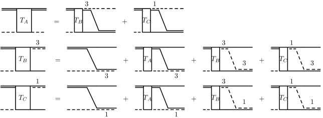
Figure 2: Integral equations for the $\Lambda nn$ system ($I=1$) and the hypertriton ($I=0$). The solid double line corresponds to a ${}^{1}S_{0}$ $(NN)$ dibaryon ($\Lambda nn$ case) or a ${}^{3}S_{1}$ $(NN)$ dibaryon (hypertriton case). The dashed-solid double lines with index 1/3 correspond to $\Lambda N$ dibaryons in the singlet/triplet channel. Single lines are as in Fig. 1.

Note that there is no tree level and no loop diagram with $T_{A}$ in the first equation.

$I=0$ channel

For the hypertriton, we correct the equation obtained in Ref. Hammer (2002) for the case $y=0$ by a factor of $1/2$ in front of the loop diagrams with $T_{C}^{I=0}$ and $T_{B}^{I=0}$. (For the case of general $y$, see Eq. (42) in Appendix A.) This factor results from the corrected dimer propagator for the $\Lambda N$ partial waves, Eq. (5). We obtain

$$\begin{split}T_{A}^{I=0}\left(k,p\right)=&-\frac{1}{2\pi}\int_{0}^{\Lambda_{c}}dqq^{2}\left[L_{B}\left(p,q,E\right)T_{B}^{I=0}\left(k,q\right)-3L_{C}\left(p,q,E\right)T_{C}^{I=0}\left(k,q\right)\right]\\ T_{B}^{I=0}\left(k,p\right)=&-\frac{4\pi\gamma_{d}}{M}L_{I}\left(p,k,E\right)-\frac{1}{\pi}\int_{0}^{\Lambda_{c}}dqq^{2}L_{A}\left(p,q,E\right)T_{A}^{I=0}(k,q)\\ &-\frac{1}{2\pi}\int_{0}^{\Lambda_{c}}dqq^{2}\left[L_{B}\left(p,q,E\right)T_{B}^{I=0}\left(k,q\right)+3L_{C}\left(p,q,E\right)T_{C}^{I=0}\left(k,q\right)\right]\\ T_{C}^{I=0}\left(k,p\right)=&\frac{4\pi\gamma_{d}}{M}L_{I}\left(p,k,E\right)+\frac{1}{\pi}\int_{0}^{\Lambda_{c}}dqq^{2}L_{A}\left(p,q,E\right)T_{A}^{I=0}(k,q)\\ &-\frac{1}{2\pi}\int_{0}^{\Lambda_{c}}dqq^{2}\left[L_{B}\left(p,q,E\right)T_{B}^{I=0}\left(k,q\right)-L_{C}\left(p,q,E\right)T_{C}^{I=0}\left(k,q\right)\right]\,,\end{split}$$ (7)

where $k$ $(p)$ denote the incoming (outgoing) momenta in the center-of-mass frame and the dependence of the amplitudes on the total energy is $E=3k^{2}\left(4M\right)-\gamma^{2}_{d}/M$ is suppressed. A cutoff $\Lambda_{c}$ is introduced in order to regulate the integral equations. The function $L_{I}$ is given by

$$L_{I}\left(p,k,E\right)=\frac{1}{pk}\ln\left(\frac{k^{2}+p^{2}+pk-ME}{k^{2}+p^{2}-pk-ME}\right)\,,$$ (8)

while the functions $L_{A/B/C}$ are

$$L_{A/B/C}\left(p,q,E\right)=\frac{1}{pq}\ln\left(\frac{q^{2}+p^{2}+pq-ME}{q^{2}+p^{2}-pq-ME}\right)\left[-\gamma_{d/3/1}+\sqrt{\frac{3}{4}q^{2}-ME-i\epsilon}\right]^{-1}\,.$$ (9)

The amplitude is normalized such that

$$T_{A}^{I=0}\left(k,k\right)=\frac{3\pi}{M}\frac{1}{k\cot{\delta}-ik}$$ (10)

with $\delta$ the elastic scattering phase shift for $\Lambda d$ scattering. For further details of the calculation and the partial wave projection, see Ref. Hammer (2002) and Appendix B.

$I=1$ channel

In the $I=1$ channel, the integral equations have a similar structure. For vanishing mass difference $y=0$, we obtain

$$\begin{split}T_{A}^{I=1}\left(k,p\right)=&\frac{1}{2\pi}\int\differential{q}q^{2}\left[3\tilde{L}_{B}\left(p,q,E\right)T_{B}^{I=1}\left(k,q\right)+\tilde{L}_{C}\left(p,q,E\right)T_{C}^{I=1}\left(k,q\right)\right]\\ T_{B}^{I=1}\left(k,p\right)=&+\frac{4\pi\gamma_{\text{nn}}}{M}L_{I}\left(p,q,E\right)+\frac{1}{\pi}\int\differential{q}q^{2}L_{A}\left(q,p,E\right)T_{A}^{I=1}\left(k,q\right)\\ &+\frac{1}{2\pi}\int\differential{q}\left[L_{B}\left(p,q,E\right)T_{B}^{I=1}\left(k,q\right)+L_{C}\left(p,q,E\right)T_{C}^{I=1}\left(k,q\right)\right]\\ T_{C}^{I=1}\left(k,p\right)=&+\frac{4\pi\gamma_{\text{nn}}}{M}L_{I}\left(p,q,E\right)+\frac{1}{\pi}\int\differential{q}q^{2}L_{A}\left(q,p,E\right)T_{A}^{I=1}\left(k,q\right)\\ &+\frac{1}{2\pi}\int\differential{q}\left[3L_{B}\left(p,q,E\right)T_{B}^{I=1}\left(k,q\right)-L_{C}\left(p,q,E\right)T_{C}^{I=1}\left(k,q\right)\right]\,,\end{split}$$ (11)

where $\gamma_{s}\equiv\gamma_{nn}$ is the dineutron pole momentum, which also replaces the deuteron pole momentum in the definition of $L_{A}$. In this case there are no bound two-body subsystems. However, we have chosen the normalization such that the scattering phase shift for scattering of a $\Lambda$ and a hypothetical bound dineutron can be obtained from $T_{A}^{I=1}$ as in Eq. (10). For further details of the calculation and the partial wave projection, see Appendix B.

IV Asymptotic analysis

In order to assess the need for a $\Lambda NN$ three-body force for proper renormalization, we perform an asymptotic analysis of the three-body equations Bedaque et al. (1999, 2000). In the asymptotic limit $\Lambda_{c}\gg q,p\gg\gamma_{d},\gamma_{nn},\gamma_{1},\gamma_{3}\sim k$ the integral equations can be solved analytically. We do this in two steps. First, we neglect the $\Lambda$-nucleon mass difference and set $y=0$. In a second step, we relax this simplification.

$I=0$ channel

In the limit $\Lambda_{c}\gg q,p\gg\gamma_{d},\gamma_{nn},\gamma_{1},\gamma_{3}\sim k$, we can neglect the inhomogeneous terms in the equations and the $k$-dependence of the amplitudes $T_{A/B/C}^{I=0}$. Setting $y=0$, the logarithmic dependences of the kernel are the same for each amplitude (see also Eq. (9)). The equations can then be written as

$$\left(\begin{array}[]{c}\tilde{T}^{I=0}_{A}\left(p\right)\\ \tilde{T}^{I=0}_{B}\left(p\right)\\ \tilde{T}^{I=0}_{C}\left(p\right)\\ \end{array}\right)=\frac{1}{2\pi}\frac{2}{\sqrt{3}}\int dq\frac{1}{q}\ln\left(\frac{p^{2}+q^{2}+pq}{p^{2}+q^{2}-pq}\right)\left(\begin{array}[]{ccc}0&-1&3\\ -2&-1&-3\\ 2&-1&1\\ \end{array}\right)\left(\begin{array}[]{c}\tilde{T}^{I=0}_{A}\left(q\right)\\ \tilde{T}^{I=0}_{B}\left(q\right)\\ \tilde{T}^{I=0}_{C}\left(q\right)\\ \end{array}\right)\,,$$ (12)

where we have defined $\tilde{T}^{I=0}_{j}\left(p\right)=pT^{I=0}_{j}\left(k\sim\gamma_{d},p\right)$ for $j\in\left\{A,B,C\right\}$. We can decouple this set of equations and obtain

$$\left(\begin{array}[]{c}T_{1}^{I=0}\\ T_{2}^{I=0}\\ T_{3}^{I=0}\\ \end{array}\right)=\frac{1}{2\pi}\frac{2}{\sqrt{3}}\int dq\frac{1}{q}\ln\left(\frac{p^{2}+q^{2}+pq}{p^{2}+q^{2}-pq}\right)\left(\begin{array}[]{ccc}-2&0&0\\ 0&-2&0\\ 0&0&4\\ \end{array}\right)\left(\begin{array}[]{c}T_{1}^{I=0}\\ T_{2}^{I=0}\\ T_{3}^{I=0}\\ \end{array}\right)\,,$$ (13)

where

$$\left(\begin{array}[]{c}\tilde{T}^{I=0}_{A}\\ \tilde{T}^{I=0}_{B}\\ \tilde{T}^{I=0}_{C}\\ \end{array}\right)=\frac{1}{12}\left(\begin{array}[]{ccc}-2&1&3\\ 2&5&3\\ 4&-2&6\\ \end{array}\right)\left(\begin{array}[]{c}T_{1}^{I=0}\\ T_{2}^{I=0}\\ T_{3}^{I=0}\\ \end{array}\right).$$ (14)

Danilov showed that a equation of the the the form Danilov (1961)

$$f\left(p\right)=\frac{4\lambda}{\sqrt{3}\pi}\int\frac{\differential{q}}{q}\ln\left(\frac{p^{2}+q^{2}+pq}{p^{2}+q^{2}-pq}\right)f\left(q\right)$$ (15)

is invariant under scale transformations and under the inversion $q\rightarrow 1/q$ and thus has power law solutions. If $\lambda<\lambda_{c}=3\sqrt{3}/\left(4\pi\right)\approx 0.4135$, the exponent of the power law is real. This is obviously fulfilled for the amplitudes $T_{1}^{I=0}$ and $T_{2}^{I=0}$. For $T_{3}^{I=0}$ on the other hand $\lambda=1$ and there are two linearly independent solutions with complex exponents, $T_{3}^{I=0}\left(k,p\right)=p^{\pm is_{0}}$. The parameter $s_{0}$ is given by the transcendental equation Danilov (1961)

$$1=\frac{8\lambda}{\sqrt{3}s}\frac{\sin\frac{\pi s}{6}}{\cos\frac{\pi s}{2}}\,,$$ (16)

resulting in $s_{0}=1.00624$ for the equal mass considered here. This corrects the result $s_{0}=1.35322$ found in Hammer (2002) due to the missing factors in Eq. (7).

The phase between the two solutions is not fixed, instead it depends strongly on the cutoff $\Lambda_{c}$. This cutoff dependence can be absorbed by adding a one-parameter three-body force $H\left(\Lambda_{c}\right)$ in the equation for $T_{3}^{I=0}$ Hammer (2002)

$$T_{3}^{I=0}\left(p\right)=\frac{4}{\sqrt{3}\pi}\int_{0}^{\Lambda_{c}}\frac{\differential{q}}{q}\left[\ln\left(\frac{p^{2}+q^{2}+pq}{p^{2}+q^{2}-pq}\right)+2H^{I=0}\left(\Lambda_{c}\right)\frac{pq}{\Lambda_{c}^{2}}\right]T_{3}^{I=0}\left(q\right).$$ (17)

This three-body force $H^{I=0}\left(\Lambda_{c}\right)$ runs with the cutoff as Bedaque et al. (1999)

$$H^{I=0}\left(\Lambda_{c}\right)=-\frac{\sin\left(s_{0}\ln\left(\frac{\Lambda_{c}}{\Lambda_{*}^{I=0}}\right)-\arctan\left(\frac{1}{s_{0}}\right)\right)}{\sin\left(s_{0}\ln\left(\frac{\Lambda_{c}}{\Lambda_{*}^{I=0}}\right)+\arctan\left(\frac{1}{s_{0}}\right)\right)}\,,$$ (18)

and ensures that all low-energy three-body observables are independent of $\Lambda_{c}$. Thus the RG evolution is covered by a limit cycle as in the triton case Bedaque et al. (2000). Due to the periodicity the value of the function $H^{I=0}\left(\Lambda_{c}\right)$ returns to its original value if the cutoff is increased by a factor $\exp\left(\pi/s_{0}\right)\approx 22.7$. The three-body-parameter $\Lambda_{*}^{I=0}$ must be fixed from a three-body input, for example the binding energy. As a consequence, there is an Efimov effect in the hypertriton channel but the spectrum is cut off in the infrared by the finite scattering length and only the shallowest state is physical.

At first glance one might think that this also fixes the three-body force in the $\Lambda nn$ system but this is not the case due to the different isospin. This three-body force can also be implemented by constructing the effective three-body Lagrangian and match the coefficients in order to achieve the behavior given by equation Eq. (17). An explicit form of the three-body term in the effective Lagrangian is shown in Appendix C.

$I=1$ channel

A similar analysis can be carried out for the $\Lambda nn$ system. With the same assumptions as before, we obtain

$$\left(\begin{array}[]{c}\tilde{T}^{I=1}_{A}\left(p\right)\\ \tilde{T}^{I=1}_{B}\left(p\right)\\ \tilde{T}^{I=1}_{C}\left(p\right)\\ \end{array}\right)=\frac{1}{2\pi}\frac{2}{\sqrt{3}}\int dq\frac{1}{q}\ln\left(\frac{p^{2}+q^{2}+pq}{p^{2}+q^{2}-pq}\right)\left(\begin{array}[]{ccc}0&3&1\\ 2&1&1\\ 2&3&-1\\ \end{array}\right)\left(\begin{array}[]{c}\tilde{T}^{I=1}_{A}\left(q\right)\\ \tilde{T}^{I=1}_{B}\left(q\right)\\ \tilde{T}^{I=1}_{C}\left(q\right)\\ \end{array}\right)\,.$$ (19)

Using the transformation

$$\left(\begin{array}[]{c}\tilde{T}^{I=1}_{A}\\ \tilde{T}^{I=1}_{B}\\ \tilde{T}^{I=1}_{C}\\ \end{array}\right)=\frac{1}{12}\left(\begin{array}[]{ccc}-2&3&5\\ -2&3&-1\\ 4&6&2\\ \end{array}\right)\left(\begin{array}[]{c}T_{1}^{I=1}\\ T_{2}^{I=1}\\ T_{3}^{I=1}\\ \end{array}\right)\,,$$ (20)

we obtain the same set of equations as for the hypertriton:

$$\left(\begin{array}[]{c}T_{1}^{I=1}\\ T_{2}^{I=1}\\ T_{3}^{I=1}\\ \end{array}\right)=\frac{1}{2\pi}\frac{2}{\sqrt{3}\pi}\int dq\frac{1}{q}\ln\left(\frac{p^{2}+q^{2}+pq}{p^{2}+q^{2}-pq}\right)\left(\begin{array}[]{ccc}4&0&0\\ 0&-2&0\\ 0&0&-2\\ \end{array}\right)\left(\begin{array}[]{c}T_{1}^{I=1}\\ T_{2}^{I=1}\\ T_{3}^{I=1}\\ \end{array}\right)\,.$$ (21)

As a consequence, the structure of the solutions is the same and the same scaling exponent $s_{0}=1.00624$ emerges. This is the well-known result for three distinguishable particles with equal masses, one neutron with spin up and down each and a $\Lambda$ Braaten and Hammer (2006). In passing, we note that our result for $s_{0}$ disagrees with the value $s_{0}=0.803$ found in Ref. Ando et al. (2015).

The three-body force $H^{I=1}$ has the same structure as in the hypertriton channel, Eq. (18), but the three-body parameter $\Lambda_{*}^{I=1}$ is not related to $\Lambda_{*}^{I=0}$ at the resolution level of pionless EFT. An explicit form of the three-body term in the effective Lagrangian is shown again in Appendix C .

Asymptotic analysis with different masses

Next we relax our assumption of equal masses and include the $\Lambda$-nucleon mass difference and repeat the analysis for finite $y$. The integral equations for this case are given in Appendices A and B. Since the logarithm in Eq. (43) depends on $y$, it can no longer be factorized out of the matrix. In the limit $y\rightarrow 0$, however, the result from the analysis above must be reproduced. Thus we assume that the $T_{i}^{I}$ can be written as a linear combination of three new amplitudes which behave as a power law

$$T_{i}^{I}=\alpha_{i}T_{1}^{I}+\beta_{i}T_{2}^{I}+\gamma_{i}T_{3}^{I}\,,\quad i\in\{A,B,C\}\,.$$ (22)

Integrating term by term and utilizing the Mellin-transform on the $y$ dependent $L_{i}$ leads to two different $y$ dependent functions,

$$F(s)= \frac{\cos\left(\phi^{+}s\right)-\cos\left(\phi^{-}s\right)}{\sin\left(\pi s\right)}\,,\mbox{\quad with\quad}\phi^{\pm}=\arccos\left(\pm\frac{\sqrt{1+y}}{2}\right)\,,$$ (23)

$$G(s)= \frac{\cos\left(\phi^{+}s\right)-\cos\left(\phi^{-}s\right)}{\sin\left(\pi s\right)}\,,\mbox{\quad with\quad}\phi^{\pm}=\arccos\left(\pm\frac{1-y}{2}\right)\,,$$ (24)

with $s$ the exponent of the of the power law ansatz. Since no amplitude is preferred by construction, the transformed integral equations decouple into three times the same subset of equations for $\alpha_{i},\beta_{i}$ and $\gamma_{i}$. Without loss of generality, we choose the subset $\gamma_{i}$ to contain the complex exponent. For $I=1$ channel, we obtain the equation

$$\left(\begin{array}[]{c}\gamma_{A}^{I=1}\\ \gamma_{B}^{I=1}\\ \gamma_{C}^{I=1}\\ \end{array}\right)=\frac{1}{s}\frac{1}{\sqrt{3-y}}\left(\begin{array}[]{ccc}0&6(y+1)^{-\frac{s+3}{2}}F&2(y+1)^{-\frac{s+3}{2}}F\\ 4(y+1)^{\frac{s+1}{2}}&\frac{2G}{\sqrt{y+1}(1-y)}&\frac{2G}{\sqrt{y+1}(1-y)}\\ 4(y+1)^{\frac{s+1}{2}}&\frac{6G}{\sqrt{y+1}(1-y)}&-\frac{2G}{\sqrt{y+1}(1-y)}\end{array}\right)\left(\begin{array}[]{c}\gamma_{A}^{I=1}\\ \gamma_{B}^{I=1}\\ \gamma_{C}^{I=1}\\ \end{array}\right)\,,$$ (25)

where the $s$-dependence of the functions $G$ and $F$ has been suppressed. This equation has only nontrivial solutions if the determinant of the matrix on its right-hand side vanishes. This leads to the following governing equation for $s$

$$16\cdot\frac{s(3-y)(y+1)\left(2F^{2}(y-1)^{2}+G^{2}\right)+8F^{2}G(1-y)\sqrt{(3-y)(y+1)}}{s^{3}(y-3)^{2}(y-1)^{2}(y+1)^{2}}=1\,.$$ (26)

In the case of the hypertriton ($I=0$), one obtains the same equation for $s$. As expected, for vanishing mass difference the result $s_{0}=1.00624$ is reproduced. The result for the scaling $\exp(\pi/s_{0})$ as a function of $M/M_{\Lambda}=\left(1-y\right)/\left(1+y\right)$ is shown in Fig. 3. For the physical value of $y=0.086$ corresponding to $M/M_{\Lambda}=0.84$, we obtain $s_{0}=1.00760$ for both the $\Lambda nn$ and hypertriton cases. Our result for arbitrary non equal masses is in good agreement with the results obtained in Ref. Braaten and Hammer (2006).

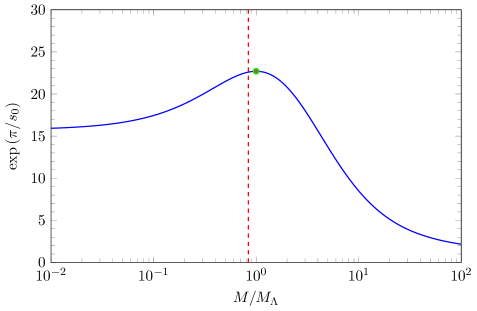
Figure 3: Scaling factor $\exp\left(\pi/s_{0}\right)$ determined by Eq. (25) as function of the mass ratio $M/M_{\Lambda}=\left(1-y\right)/\left(1+y\right)$. The physical value is indicated by the dashed red line. The value for $y=0$ is given by the green dot.

Renormalization

In order to check the validity of our asymptotic analysis and the proper renormalization of the three-body equations, we calculate the three-body force for the hypertriton and the $\Lambda nn$ system numerically. The results are shown in Fig. 4. The points represent our numerical results while the straight lines are fits to the theoretical expression, Eq. (18). We use the binding energy as three-body input. The respective results for the three-body parameter $\Lambda_{*}$ are

hypertriton: $$\qquad B_{3}^{\Lambda}=2.35\, \text{MeV}\,, \quad\Lambda_{*}^{I=0}=(6.372\pm 0.008)\, \text{MeV}\,,$$

$$\Lambda nn: \qquad B_{\Lambda nn}=1.1\; \text{MeV}\,, \quad\Lambda_{*}^{I=1}=(13.95\pm 0.02) \text{MeV}\,.$$ (27)

The three-body force $H$ is the determined numerically such that the binding energy remains fixed as the cutoff $\Lambda_{c}$ is varied. In both cases, the three-body force shows the expected limit cycle behavior. Therefore three-body states generated by the Efimov effect can be expected for $I=0$ and $I=1$.

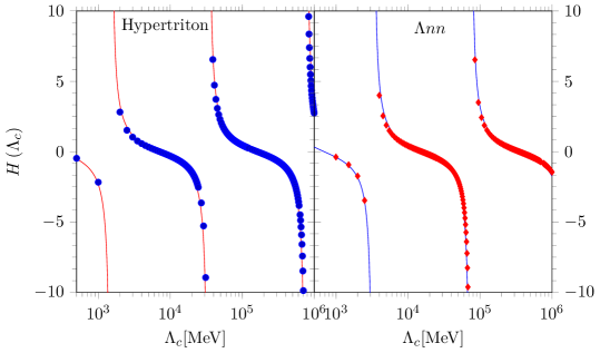
Figure 4: Three-body force $H(\Lambda_{c})$ for the hypertriton (left panel) and the $\Lambda nn$ system (right panel) as a function of the cutoff $\Lambda_{c}$. The points are numerical determinations obtained from taking the three-body binding energy as input (cf. Eq. (27)), while the solid lines are fits to Eq. (18).

For inclusion of the three-body force in leading-order calculations it is convenient to choose cutoff values at which the three-body force vanishes Hammer and Mehen (2001):

$$\Lambda_{n}=\Lambda_{*}\exp\left[\frac{1}{s_{0}}\left(n\pi+\arctan\left(\frac{1}{s_{0}}\right)\right)\right]\,,$$ (28)

with $n>0$ an integer. In the following, Eq. (28) with $n=1$ is used for all numerical calculations.

V Numerical Results

In order to solve the integral equations for the $\Lambda nn$ system or the hypertriton we need to set the interaction parameters. For the spin-triplet nucleon-nucleon interaction, which contributes in the $I=0$ channel, we take the deuteron binding momentum $\gamma_{d}=45.68$ MeV as input. For the spin-singlet interaction, we take the value for neutron-neutron scattering length, $a_{\text{nn}}=-18.63\pm 0.10\,$(stat.)$\pm 0.44\,$(syst.)$\pm 0.30\,$(theo.) fm  Chen et al. (2008), since we focus explicitly on the $\Lambda nn$ system in this channel. The values for the $\Lambda N$ S-wave interaction can not be extracted from phase shift analyses of the limited scattering data. Instead, we use the NLO chiral EFT values Haidenbauer et al. (2013) for all calculations in this work, i.e. $a^{\Lambda p}_{s}=-2.91$ fm and $a^{\Lambda p}_{t}=-1.61$ fm for the spin-singlet and spin-triplet channels, respectively.

$I=0$ channel

The $\Lambda d$ scattering phase is shown in Fig. 5. The dark blue/red band is a variation of the chiral EFT scattering lengths $a^{\Lambda p}_{s}=-2.91$ fm and $a^{\Lambda p}_{t}=-1.61$ fm by 15 percent, which covers the entire predicted range, therefore the scattering phase shifts seems to be independent from the exact values of the low $\Lambda N$ scattering lengths for small momenta. Small deviations occur closer to the deuteron breakup threshold. The hatched bands give an estimate of the pionless EFT error at this order.

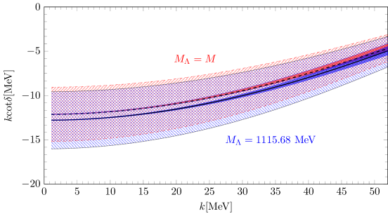
Figure 5: $\Lambda-d$ scattering phase shifts for $y=0$ (dashed red line) and physical value of the $\Lambda$ mass (black solid line). The dark blue/red bands represent the sensitivity to a variation of the chiral EFT input scattering lengths by 15%, while the blue/red hatched bands give an estimate of the EFT error.

The large scattering lengths induce universal correlation between different observables. One prominent example is the Phillips line, which was first observed in deuteron-neutron system Phillips (1968). The Phillips line is a correlation between the $nd$ S-wave scattering length and the triton binding energy. A similar correlation occurs in the hypertriton channel Hammer (2002). The Phillips line for the hypertriton is shown in Fig. 6 for both the equal mass case (green dashed line) and for the physical $\Lambda$ mass (blue solid line). The correlation shows the expected behavior with $a_{\Lambda d}$ going to infinity as $B_{3}^{\Lambda}$ approaches the deuteron binding energy. The EFT is expected to break down when the three-body binding momentum is of the order of the pion mass, corresponding to $B_{3}^{\Lambda}\gtrsim 8\gamma_{d}^{2}/M\approx 18$ MeV (grey shaded area). The Phillips line correlation is not very sensitive to the precise values of the the $\Lambda N$ scattering lengths. This is illustrated by the different black symbols in Fig. 6 showing the sensitivity to changes in $\gamma_{i}=1/a_{i}$, where $i=1,3$ with the range of applicability of the theory. Such a behavior is not completely unexpected since the $\Lambda d$ separation energy is very small.

From the hypertriton binding energy, the $\Lambda d$ scattering is predicted as

$$a_{\Lambda d}^{y=0}=16.25^{+4.45}_{-2.40}\,\text{fm}\,,\qquad a_{\Lambda d}^{y=0.086}=15.4^{+4.3}_{-2.3}\,\text{fm}\,$$ (29)

where the error is determined by the uncertainty in the hypertriton binding energy. The change from finite $y$ is of order 15%, well within errors of this LO calculation. The value for the equal mass case, $y=0$, is in good agreement with the previous work in Refs. Cobis et al. (1997); Hammer (2002).

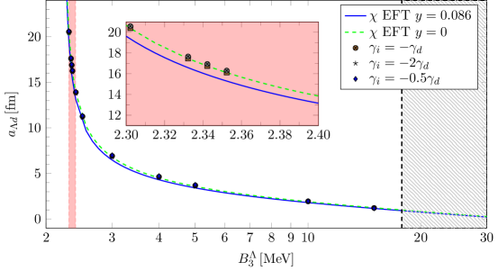
Figure 6: Phillips line for the hypertriton for $y=0$ (dashed green line) and physical $\Lambda$ mass (solid blue line). In the gray shaded area the EFT description breaks down, while the red shaded area represents the physical binding energy region and is enhanced in the inset. The different black symbols in illustrate the sensitivity to changes in $\gamma_{i}=1/a_{i}$, where $i=1,3$.

$I=1$ channel

The question of whether the $\Lambda nn$ system is bound or not has not been answered conclusively. After regularization pionless EFT always produces one (or more) bound states in the $\Lambda nn$ system for a sufficiently large value of the cutoff $\Lambda$. Yet such bound states are only physically relevant if they lie below the breakdown scale of the EFT. Since we do not have any three-body information besides the HypHI experiment, we can not make a conclusive statement about the existence of such a state. Assuming a flat probability distribution for possible values of $\Lambda_{*}^{I=1}$ generated by QCD and deformations of QCD in the relevant parameter window (one cycle), we can make a statistical estimate. Taking into account the relevant thresholds, we estimate the probability $P$ of finding a bound $\Lambda nn$ from the ratio of the allowed values for $\Lambda_{*}^{I=1}$ for a $\Lambda nn$ state below the breakdown scale and a whole cycle,

$$P=\frac{\Lambda_{*}^{I=1,\text{breakdown}}-\Lambda_{*}^{I=1,\text{threshold}}}{(e^{\pi/s_{0}}-1)\Lambda_{*}^{I=1,\text{threshold}}}\leavevmode\nobreak\ .$$ (30)

Under these assumptions, we estimate that there is a 6% chance to find a $\Lambda nn$ bound state within in the range of pionless EFT, which breaks down for typical momenta of the order of the pion mass. We note that this simple estimate does not take into account any constraints from other nuclear and hypernuclear observables and/or theory assumptions beyond pionless EFT. In the case of the hypertriton, we would estimate a probability of order 20% using the same method.

For illustrative purposes, we also discuss the Phillips line correlation for a hypothetical bound dineutron (${}^{2}n$) Hammer and König (2014). The accepted value for the neutron-neutron scattering length is $a_{nn}=-18.63$ fm Chen et al. (2008) but experiments are primarily sensitive absolute value of the scattering length, such that the sign is mainly determined by the non-observation of a bound dineutron and theoretical considerations about charge symmetry breaking Gardestig (2009). The corresponding Phillips line correlation for the $\Lambda$-dineutron system is shown in Fig. 7.

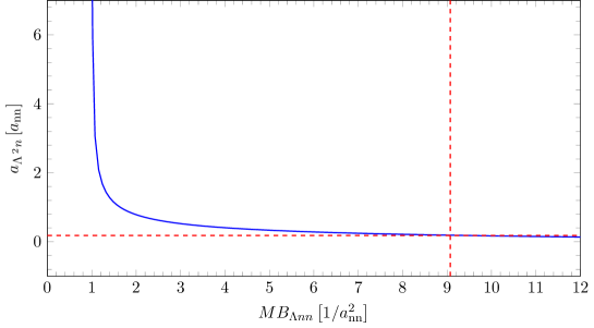
Figure 7: Phillips line for the $\Lambda nn$ system in the case of a hypothetical bound dineutron for arbitrary positive values of $a_{nn}$. The extracted mass of the $\Lambda nn$ system by the HypHI collaboration Rappold et al. (2013) and the corresponding $\Lambda$-dineutron scattering length for a hypothetical value $a_{nn}=18.63$ fm are marked by dashed lines.

The correlation again shows the expected behavior for low binding momenta and the $\Lambda$-dineutron scattering length diverges as the dineutron binding energy is approached. The scattering length associated with the extracted value of the $\Lambda nn$ binding energy $B_{\Lambda nn}=1.1$ MeV Rappold et al. (2013) for the hypothetical value $a_{nn}=18.63$ fm is very low. This is expected since the binding of the $\Lambda$-dineutron system must be very tight. (The dineutron binding energy $B_{nn}=1/(Ma^{2}_{nn})\approx 0.12$ MeV is very small for this example.) The point of expected theory break down is far away from the displayed area in Fig. 7.

VI Wave functions and matter radii

$I=0$ channel

In this section, we discuss the structure of the hypertriton and $\Lambda nn$ states and calculate their wave functions and matter radii. A discussion of hypertriton structure as a loosely bound object of a $\Lambda$ and a deuteron in the context of heavy ion collisions at the LHC can be found in Braun-Munzinger and Dönigus (2018); Chen et al. (2018).

Using the integral equations for scattering in the hypertriton channel, we can obtain the bound state equation by dropping the inhomogeneous terms and the $k$-dependence of the amplitudes. For further calculations its useful to use Jacobi coordinates in momentum space. Hence we use momentum plane-wave states $\ket{p,q}_{i}$. These plane-wave state momenta are defined in the two-body fragmentation channel $(i,jk)$. The particle $i$ is the spectator while the particles $j$ and $k$ are interacting with each other Faddeev (1961); Afnan and Thomas (1977); Glöckle (1983). Therefore the momentum $\mathbf{p}$ describes the relative momentum between the interacting pair while $q$ is the relative momentum between the spectator and the interacting-pair center of mass. The projection between the different spectators (nucleons ($N$) and Lambda-particle ($\Lambda$)) must obey

$${}_{N}\innerproduct{\mathbb{p}\mathbb{q}}{\mathbb{p}^{\prime}\mathbb{q}^{\prime}}_{\Lambda} =\left(2\pi\right)\delta^{(3)}\left(\mathbb{p}+\boldsymbol{\pi}_{1}\left(\mathbb{q^{\prime}},\mathbb{q}\right)\right)\delta^{(3)}\left(\mathbb{p^{\prime}}-\boldsymbol{\pi}_{2}\left(\mathbb{q},\mathbb{q^{\prime}}\right)\right)\leavevmode\nobreak\ ,$$ (31)

$${}_{N}\matrixelement{\mathbb{p}\mathbb{q}}{\mathcal{P}}{\mathbb{p}^{\prime}\mathbb{q}^{\prime}}_{N} =\left(2\pi\right)\delta^{(3)}\left(\mathbb{p}+\boldsymbol{\pi}_{3}\left(\mathbb{q^{\prime}},\mathbb{q}\right)\right)\delta^{(3)}\left(\mathbb{p^{\prime}}-\boldsymbol{\pi}_{3}\left(\mathbb{q},\mathbb{q^{\prime}}\right)\right)\leavevmode\nobreak\ .$$ (32)

The Operator $\mathcal{P}$ denotes the permutation of the two nucleons. The momentum functions are

$$\begin{split}\boldsymbol{\pi}_{1}\left(\mathbb{q},\mathbb{q}^{\prime}\right)&=\mathbb{q}+\frac{1+y}{2}\mathbb{q}^{\prime}\leavevmode\nobreak\ ,\\ \boldsymbol{\pi}_{2}\left(\mathbb{q},\mathbb{q}^{\prime}\right)&=\mathbb{q}+\frac{1}{2}\mathbb{q}^{\prime}\leavevmode\nobreak\ ,\\ \boldsymbol{\pi}_{3}\left(\mathbb{q},\mathbb{q}^{\prime}\right)&=\mathbb{q}+\frac{1-y}{2}\mathbb{q}^{\prime}\leavevmode\nobreak\ ,\\ \end{split}$$ (33)

where $y$ is again the mass parameter. Starting form the hypertriton bound state equations, we obtain the wave functions for different spectators by adding dimer and one-particle propagators to the transition amplitudes. This leads to the wavefunction given in Eq. (34) Hammer et al. (2017); Acharya et al. (2013); Canham and Hammer (2008). The cosine of the angle between the two momenta $\mathbb{p}$ and $\mathbb{q}$ is given by $x$. In principle, higher partial waves arise at this point, however, in the S-wave case they are negligibly small Göbel et al. (2019). The prefactors result from projecting onto spin $S=1/2$:

$$\begin{split}\Psi_{\Lambda}\left(p,q\right)=&G_{\Lambda}\left(p,q,B\right)\left[D_{D}\left(q,B\right)T_{A}\left(q\right)-\frac{1}{2}\int_{-1}^{1}\differential{x}D_{3}\left(\pi_{2}\left(\mathbb{p},-\mathbb{q}\right),B\right)T_{B}\left(\pi_{2}\left(\mathbb{p},-\mathbb{q}\right)\right)\right.\\ &\left.+\frac{3}{2}\int_{-1}^{1}\differential{x}D_{1}\left(\pi_{2}\left(\mathbb{p},-\mathbb{q}\right),B\right)T_{1}\left(\pi_{2}\left(\mathbb{p},-\mathbb{q}\right)\right)\right]\,,\end{split}$$

$$\begin{split}\Psi_{N}\left(p,q\right)=&G_{n}\left(p,q,B\right)\left[D_{3}\left(q,B\right)T_{B}\left(q\right)-\frac{1}{2}\int_{-1}^{1}\differential{x}D_{D}\left(\pi_{1}\left(\mathbb{p},-\mathbb{q}\right),B\right)T_{A}\left(\pi_{1}\left(\mathbb{p},-\mathbb{q}\right)\right)\right.\\ &\left.-\frac{1}{2}\int_{-1}^{1}\differential{x}D_{3}\left(\pi_{3}\left(\mathbb{p},-\mathbb{q}\right),B\right)T_{B}\left(\pi_{3}\left(\mathbb{p},-\mathbb{q}\right)\right)-\frac{3}{2}\int_{-1}^{1}\differential{x}D_{1}\left(\pi_{3}\left(\mathbb{p},-\mathbb{q}\right),B\right)T_{1}\left(\pi_{3}\left(\mathbb{p},-\mathbb{q}\right)\right)\right]\,,\\ \Psi_{N^{\prime}}\left(p,q\right)=&G_{n}\left(p,q,B\right)\left[D_{1}\left(q,B\right)T_{B}\left(q\right)+\frac{1}{2}\int_{-1}^{1}\differential{x}D_{D}\left(\pi_{1}\left(\mathbb{p},-\mathbb{q}\right),B\right)T_{A}\left(\pi_{1}\left(\mathbb{p},-\mathbb{q}\right)\right)\right.\\ &\left.-\frac{1}{2}\int_{-1}^{1}\differential{x}D_{3}\left(\pi_{3}\left(\mathbb{p},-\mathbb{q}\right),B\right)T_{B}\left(\pi_{3}\left(\mathbb{p},-\mathbb{q}\right)\right)+\frac{1}{2}\int_{-1}^{1}\differential{x}D_{1}\left(\pi_{3}\left(\mathbb{p},-\mathbb{q}\right),B\right)T_{1}\left(\pi_{3}\left(\mathbb{p},-\mathbb{q}\right)\right)\right]\,.\end{split}$$ (34)

The Green’s functions $G_{0}^{i}\left(p,q,B\right)$ are given by

$$\begin{split}G_{\Lambda}\left(p,q,B\right)&=\left[mB+p^{2}+\frac{3-y}{\left(1+y\right)4}q^{2}\right]^{-1}\,,\\ G_{n}\left(p,q,B\right)&=\left[mB\left(1+y\right)+p^{2}+\frac{3-y}{4}q^{2}\right]^{-1}\,.\\ \end{split}$$ (35)

The absolute square of the spectator wave functions is shown on a logarithmic scale in Fig. 8.

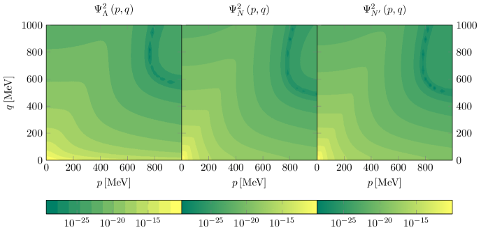
Figure 8: The absolute square of the wave functions $\Psi^{2}_{\Lambda}\left(p,q\right),\leavevmode\nobreak\ \Psi_{N}^{2}\left(p,q\right)$ and $\Psi^{2}_{N^{\prime}}\left(p,q\right)$ (normalized to one). The $z$ axis is logarithmic; $p$ describes the momentum between the interacting pair while $q$ describes the momentum between the spectator and the interacting pair.

Starting from there we can calculate one-body matter-density form factors

$$F_{i}\left(\mathbb{k}^{2}\right)=\int\differential[3]{p}\int\differential[3]{q}\Psi_{i}\left(p,q\right)\Psi_{i}\left(p,\absolutevalue{\mathbb{q}-\mathbb{k}}\right),$$ (36)

where $i$ is again the spectator. Matter radii then can be extracted by expanding the form factors in terms of $\mathbb{k^{2}}$ leading to the relation

$$F_{i}\left(\mathbb{k}^{2}\right)=1-\frac{1}{6}\mathbb{k}^{2}\langle r^{2}_{i-jk}\rangle+\ldots\leavevmode\nobreak\ ,$$ (37)

where $\langle r^{2}_{i-jk}\rangle$ denotes the mean square distance between the spectator and the interacting pair center on mass Hammer et al. (2017). An overview over the different radii corresponding to different form factors is shown in Fig. 9. The form factor $F_{jk}\left(\mathbb{k}^{2}\right)$ is given by

$$F_{jk}\left(\mathbb{k}^{2}\right)=\int\differential[3]{p}\int\differential[3]{q}\Psi_{i}\left(p,q\right)\Psi_{i}\left(\absolutevalue{\mathbb{p}-\mathbb{k}},q\right).$$ (38)

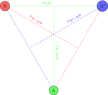
radius	corresponding form factor
$\langle r_{\Lambda-NN^{\prime}}^{2}\rangle$	$F_{\Lambda}\left(\mathbb{k}^{2}\right)$
$\langle r_{N-\Lambda N^{\prime}}^{2}\rangle$	$F_{N}\left(\mathbb{k}^{2}\right)$
$\langle r_{N^{\prime}-\Lambda N}^{2}\rangle$	$F_{N^{\prime}}\left(\mathbb{k}^{2}\right)$
$\langle r_{NN^{\prime}}^{2}\rangle$	$F_{NN^{\prime}}\left(\mathbb{k}^{2}\right)$

Figure 9: Different matter radii for the $\Lambda NN$ systems and the corresponding form factors.

Since, we consider a tightly bound proton-neutron compared to the binding energy of the $\Lambda$ particle to the pair, we expect the results to be close to treating the system as a two-body state. A first estimate is given by considering a shallow S-wave two-body bound state resulting in

$$B_{2}=\frac{1}{2\mu a^{2}}\mbox{\quad and\quad}\langle r^{2}\rangle=\frac{a^{2}}{2}\leavevmode\nobreak\ ,$$ (39)

where $\mu$ is the two-body reduced mass Braaten and Hammer (2006). Using these two equations, we can get an estimate for the two radii

$$\sqrt{\langle r^{2}_{NN^{\prime}}\rangle}\approx 3.04\>\text{fm}\mbox{\quad and\quad}\sqrt{\langle r^{2}_{\Lambda-NN^{\prime}}\rangle}\approx 10.34\>\text{fm}\leavevmode\nobreak\ .$$ (40)

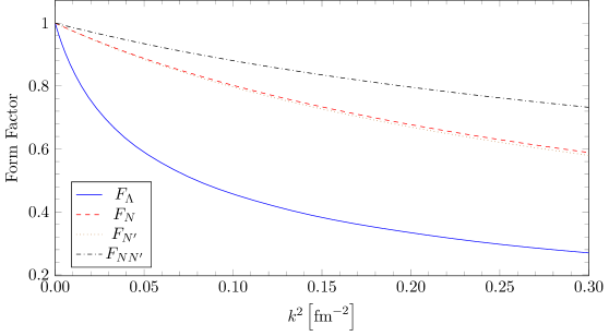
Figure 10: The Formfactors $F_{i}$ and $F_{N}$ as a function of $k^{2}$. The lines for $F_{N}$ and $F_{N^{\prime}}$ are close to each other.For identical spin-triplet and spin-singlet $\Lambda-N$ scattering lengths $F_{N}$ and $F_{N^{\prime}}$ would fall on top of each other.

The results for the different form factors are shown in Fig. 10. It is also possible to combine those radii to a geometric matter radius given by

$$\langle r^{2}_{m}\rangle=\frac{\left(A+1\right)^{2}}{\left(A+2\right)^{3}}\langle r^{2}_{N^{\prime}-\Lambda N}\rangle+\frac{\left(A+1\right)^{2}}{\left(A+2\right)^{3}}\langle r^{2}_{N-\Lambda N^{\prime}}\rangle+\frac{4A}{\left(A+2\right)^{3}}\langle r^{2}_{\Lambda-NN^{\prime}}\rangle\leavevmode\nobreak\ ,$$ (41)

where $A=M_{\Lambda}/M$ is the $\Lambda$-nucleon mass ratio. The results are shown in Table 1. We have fitted the linear part of the form factors shown in Fig. 10 close to $k^{2}=0$. The errors are mainly given by the uncertainties of the binding energy of the system rather then the uncertainties of the $\Lambda N$ scattering lengths. Comparing the three-body resultsfor $\sqrt{\langle r^{2}_{NN^{\prime}}\rangle}$ and $\sqrt{\langle r^{2}_{\Lambda-NN^{\prime}}\rangle}$ given in Table 1 with the two-body ones in Eq. (40), confirms that the ”picture” as a two body system consisting of a deuteron and a $\Lambda$ is a good approximation.

Table 1: Different matter radii for the hypertriton in fm. The first row is for the binding Energy of $2.35$ MeV with the chiral EFT predictions for the $\Lambda N$ interactions. Further rows are corrections to this value given by variations in the binding energy and $\Lambda N$ interactions.

$\sqrt{\langle r^{2}_{\Lambda-NN^{\prime}}\rangle}$[fm]	$\sqrt{\langle r^{2}_{N^{\prime}-\Lambda N}\rangle}$[fm]	$\sqrt{\langle r^{2}_{N-N^{\prime}\Lambda}\rangle}$[fm]	$\sqrt{\langle r^{2}_{NN^{\prime}}\rangle}$[fm]	$\sqrt{\langle r^{2}_{geo}\rangle}$[fm]
$10.79$	$3.96$	$4.02$	$2.96$	$4.66$
${+3.04}/{-1.53}$	${+0.40}/{-0.25}$	${+0.41}/{-0.25}$	${+0.06}/{-0.05}$	${+1.19}/{-0.54}$
${+0.03}/{-0.02}$	${+0.03}/{-0.03}$	${+0.03}/{-0.03}$	${+0.03}/{-0.04}$	${+0.01}/{-0.01}$

$I=1$ channel

Utilizing the same prescription as before, we obtain equations for the wave functions and matter radii for the $\Lambda nn$ system. The binding energy of the $\Lambda nn$ system is not known, but the invariant mass distributions suggest a binding energy of $B_{\Lambda nn}=1.1$ MeV Rappold et al. (2013). This is much larger than the $\Lambda$-deuteron separation energy of $0.13\pm 0.05$ MeV, which implies that the radii of the $\Lambda nn$ state should be smaller. We therefore calculate the matter form factors for the $\Lambda nn$ system for this value of $B_{\Lambda nn}$. Our results for the wave functions and form factors are shown in Figs. 11 and 12, respectively.

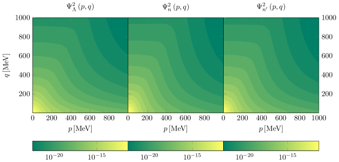
Figure 11: The absolute square of the wave functions $\Psi^{2}_{\Lambda}\left(p,q\right),\leavevmode\nobreak\ \Psi_{n}^{2}\left(p,q\right)$ and $\Psi^{2}_{n^{\prime}}\left(p,q\right)$ for the $\Lambda nn$ bound with a binding energy $B_{\Lambda nn}=1.1$ MeV. The $z$ axis is logarithmic; $p$ describes the momentum between the interacting pair while $q$ describes the momentum between the spectator and the interacting pair.

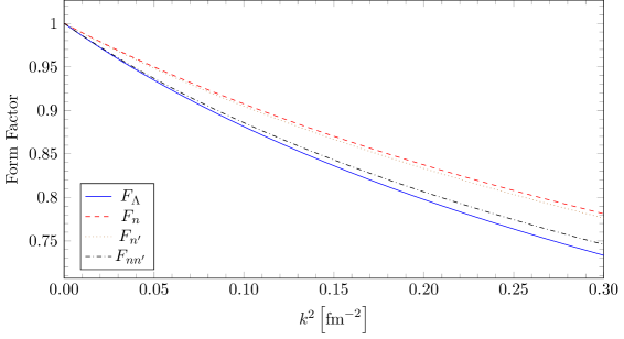
Figure 12: The Formfactors $F_{i}$ and $F_{nn}$ as a function of $k^{2}$ for the $\Lambda nn$ system. The form factors of $F_{n}$ and $F_{n^{\prime}}$ are again close to each other. For identical spin-triplet and spin-singlet $\Lambda-N$ scattering lengths $F_{n}$ and $F_{n^{\prime}}$ would fall on top of each other.

As expected the $\Lambda nn$ system does not show the two-body halo character of the hypertriton since it does not have a bound two-body subsystem. Moreover all matter radii are of comparable size.

Since the value of the $\Lambda nn$ binding energy is uncertain, we calculate the matter radii as a function of $B_{\Lambda nn}$. The results for the different radii as a function of the $\Lambda nn$ binding energy (but keeping the $NN$ and $\Lambda N$ interaction fixed) are shown in Fig. 13. The bands represent a deviation of the chiral EFT $\Lambda N$ scattering length values by $15\%$ around the central value.

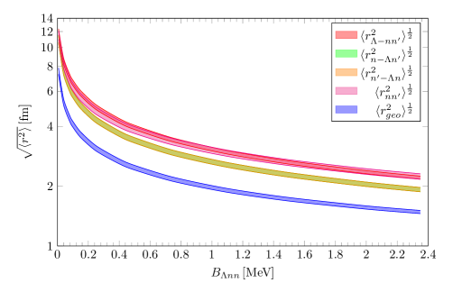
Figure 13: Matter radii for the $\Lambda nn$ system as function of the binding energy $B_{\Lambda nn}$ for a neutron-neutron scattering length of $-18.63$ fm and chiral EFT values for the $\Lambda n$ scattering lengths $\pm 15\%$ . The band for the radii with the two nucleons as spectator lie on top of each other.

The general observation that all matter radii are of comparable size continues to hold if $B_{\Lambda nn}$ is varied.

VII Summary

In this work, we have discussed the structure of three-body $S=-1$ hypernuclei in pionless EFT with a focus on the hypertriton ($I=0$) and the hypothetical $\Lambda nn$ bound state in the $I=1$ channel. Both systems show the Efimov effect and have the same scaling factor, such that the occurrence of bound states is natural within pionless EFT. However, the three-body parameters need not be the same. This is in contrast to other approaches which implicitly make assumptions about the relation between the two-channels Gal and Garcilazo (2014); Garcilazo and Valcarce (2014); Richard et al. (2015); Gal and Garcilazo (2014); Hiyama et al. (2014); Downs and Dalitz (1959). However, due to the finite scattering lengths, a physical state will only appear in the $I=1$ channel if it is within the range of validity of the pionless EFT description, i.e. if it is shallow enough. Based on our leading order analysis, we cannot rule out a $\Lambda nn$ bound state. From a simple statistical argument, we estimate that there is a 6% chance to find a $\Lambda nn$ bound state within in the range of pionless EFT.

In addition, we perform a detailed analysis of the structure of the hypertriton and the hypothetical $\Lambda nn$ bound state and related scattering processes. While the $NN$ interaction parameters are well known, the $\Lambda N$ parameters are taken from a chiral EFT analysis at NLO Haidenbauer et al. (2013). For $\Lambda d$ scattering system, we predict a scattering length length of $a^{0.086}_{\Lambda d}=15.4^{+4.3}_{-2.3}$ fm. This result is insensitive to the details of the $\Lambda N$ interaction and mainly driven by the value of the hypertriton binding energy Hammer (2002)

Moreover, we have performed calculations of matter radii and wave functions in both isospin channels. For the hypertriton, the calculation shows a large separation between the $\Lambda$ and the ”deuteron” core of $10.79^{+3.04}_{-1.53}$ fm, which is also reflected in the $\Lambda$-deuteron separation energy of only $0.13\pm 0.05$ MeV. This separation is comparable to the one obtained in a straight two-body calculation with $\Lambda$ and deuteron degrees of freedom, which lends further credibility to an effective two-body description in the case of the hypertriton Congleton (1992). Again these results are insensitive to the exact values of the $\Lambda N$ scattering lengths. Since the $\Lambda nn$ system lacks a bound two-body subsystem, this behavior is not observable for a hypothetical bound state in the $I=1$ channel. Although the question whether the $\Lambda nn$ system is bound can not be answered definitely, we are able to predict matter radii and wave functions for this system as a function of its binding energy.

In the future, it would be worthwhile to include effective range corrections and explore the usefulness of this framework to shed light on the the hypertriton lifetime puzzle (see Ref. Gal and Garcilazo (2019) and references therein).In addition, an impact analysis of the two-body scattering lengths and three-body binding energies in four-body hyper-nuclei similar to Ref. Contessi et al. (2019) would be worthwhile. Moreover, it would be interesting to include the full three-body structure of the hypertriton wave function in coalescence models for production in heavy ion collisions Zhang and Ko (2018); Braun-Munzinger and Dönigus (2018). Finally, one could combine pionless EFT with input from lattice QCD calculations in the $S=-1$ sector Beane et al. (2013) to elucidate the structure of hypernuclei at unphysical pion masses Barnea et al. (2015).

Appendix A Hypertriton integral equations

The integral equations for the hypertriton for general mass ratios $y\neq 0$ are

$$\begin{split}T_{A}^{I=0}\left(k,p\right)=&-\frac{1}{2\pi\left(1+y\right)}\int_{0}^{\Lambda_{c}}dqq^{2}\left[\tilde{L}_{B}\left(p,q,E\right)T_{B}^{I=0}\left(k,q\right)-3\tilde{L}_{C}\left(p,q,E\right)T_{C}^{I=0}\left(k,q\right)\right]\\ T_{B}^{I=0}\left(k,p\right)=&-\frac{4\pi\gamma_{d}}{M}L_{I}\left(p,k,E\right)-\frac{1}{\pi}\int_{0}^{\Lambda_{c}}dqq^{2}L_{A}\left(p,q,E\right)T_{A}^{I=0}(k,q)\\ &-\frac{1}{2\pi\left(1-y\right)}\int_{0}^{\Lambda_{c}}dqq^{2}\left[L_{B}\left(p,q,E\right)T_{B}^{I=0}\left(k,q\right)+3L_{C}\left(p,q,E\right)T_{C}^{I=0}\left(k,q\right)\right]\\ T_{C}^{I=0}\left(k,p\right)=&\frac{4\pi\gamma_{d}}{M}L_{I}\left(p,k,E\right)+\frac{1}{\pi}\int_{0}^{\Lambda_{c}}dqq^{2}L_{A}\left(p,q,E\right)T_{A}^{I=0}(k,q)\\ &-\frac{1}{2\pi\left(1-y\right)}\int_{0}^{\Lambda_{c}}dqq^{2}\left[L_{B}\left(p,q,E\right)T_{B}^{I=0}\left(k,q\right)-L_{C}\left(p,q,E\right)T_{C}^{I=0}\left(k,q\right)\right]\leavevmode\nobreak\ ,\end{split}$$ (42)

where in addition to the corrected factor of two, also the sign in the prefactor of the integral in the first equation was flipped $(1-y)\to(1+y)$. Details on the derivation are given in Ref. Hammer (2002). (See also the discussion for the $I=1$ case in Appendix B.) The $y$-dependent functions $L(p,q,E,(y))$ are given by

$$\begin{split}L_{I}&=\frac{1}{pk}\ln\left(\frac{k^{2}/(1+y)+p^{2}+pk-ME}{k^{2}/(1+y)+p^{2}-pk-ME}\right)\\ L_{A}&=\frac{1}{pq}\ln\left(\frac{q^{2}/(1+y)+p^{2}+pq-ME}{q^{2}/(1+y)+p^{2}-pq-ME}\right)\left[-\gamma_{d/s}+\sqrt{\frac{3-y}{4\left(1+y\right)}q^{2}-ME-i\epsilon}\right]^{-1}\\ \tilde{L}_{B/C}&=\frac{1}{pq}\ln\left(\frac{q^{2}+p^{2}/(1+y)+pq-ME}{q^{2}+p^{2}/(1+y)-pq-ME}\right)\left[-\gamma_{3/1}+\sqrt{\frac{3+2y-y^{2}}{4}q^{2}-ME(1+y)-i\epsilon}\right]^{-1}\\ L_{B/C}&=\frac{1}{pq}\ln\left(\frac{q^{2}+p^{2}+pq(1-y)-ME(1+y)}{q^{2}+p^{2}-pq(1-y)-ME(1+y)}\right)\left[-\gamma_{3/1}+\sqrt{\frac{3+2y-y^{2}}{4}q^{2}-ME(1+y)-i\epsilon}\right]^{-1}.\\ \end{split}$$ (43)

Appendix B $\Lambda nn$ integral equations

Starting from the Lagrangian (3) and using the same conventions and definitions for the $L_{i}$ as for the hypertriton, we obtain from the Feynman diagrams in Fig. 2 the following equations:

$$\begin{split}\left[t_{A}^{ij}\left(\vec{k},\vec{p}\right)_{\alpha\beta}\right]=&g_{s}g_{3}\int\frac{\differential[3]{q}}{\left(2\pi\right)^{3}}\left[t_{B}^{i,l^{\prime}}\left(\vec{k},\vec{q}\right)_{\alpha\beta^{\prime}}^{a^{\prime}b^{\prime}}\right]\frac{\left(\sigma_{l^{\prime}}\right)_{\beta^{\prime}\beta}\left(\tau_{j}\tau_{2}\right)_{b^{\prime}a^{\prime}}D_{3}\left(E-\frac{q^{2}}{2m},\vec{q}\right)}{E-\frac{p^{2}}{2M_{\Lambda}}-\frac{q^{2}}{2M}-\frac{\left(\vec{q}+\vec{p}\right)^{2}}{2M}+i\epsilon}\\ &+g_{s}g_{1}\int\frac{\differential[3]{q}}{\left(2\pi\right)^{3}}\left[t_{C}^{i}\left(\vec{k},\vec{q}\right)_{\alpha\beta^{\prime}}^{a^{\prime}b^{\prime}}\right]\frac{\delta_{\beta^{\prime}\beta}\left(\tau_{j}\tau_{2}\right)_{b^{\prime}a^{\prime}}D_{1}\left(E-\frac{q^{2}}{2m},\vec{q}\right)}{E-\frac{p^{2}}{2M_{\Lambda}}-\frac{q^{2}}{2M}-\frac{\left(\vec{q}+\vec{p}\right)^{2}}{2M}+i\epsilon}\\ \end{split}$$ (44)

$$\begin{split}\left[t_{B}^{i,l}\left(\vec{k},\vec{q}\right)_{\alpha\beta}^{ab}\right]=&-g_{s}g_{3}\frac{\left(\sigma_{l}\right)_{\alpha\beta}\left(\tau_{2}\tau_{i}\right)_{ab}}{E-\frac{k^{2}}{2M_{\Lambda}}-\frac{p^{2}}{2m}-\frac{\left(\vec{k}+\vec{p}\right)^{2}}{2M}+i\epsilon}\\ &+g_{s}g_{3}\int\frac{\differential[3]{q}}{\left(2\pi\right)^{3}}\left[t_{A}^{i,j^{\prime}}\left(\vec{k},\vec{q}\right)_{\alpha\beta^{\prime}}\right]\frac{\left(\sigma_{l}\right)_{\beta^{\prime}\beta}\left(\tau_{2}\tau_{j^{\prime}}\right)_{ab}D_{d}\left(E-\frac{q^{2}}{2m},\vec{q}\right)}{E-\frac{p^{2}}{2M}-\frac{q^{2}}{2M_{\Lambda}}-\frac{\left(\vec{q}+\vec{p}\right)^{2}}{2M}+i\epsilon}\\ &+g_{3}^{2}\int\frac{\differential[3]{q}}{\left(2\pi\right)^{3}}\left[t_{B}^{i,l^{\prime}}\left(\vec{k},\vec{q}\right)_{\alpha\beta^{\prime}}^{a^{\prime}b^{\prime}}\right]\frac{\left(\sigma_{l}\sigma_{l^{\prime}}\right)_{\beta^{\prime}\beta}\delta_{b^{\prime}b}\delta_{a^{\prime}a}D_{3}\left(E-\frac{q^{2}}{2m},\vec{q}\right)}{E-\frac{p^{2}+q^{2}}{2M}-\frac{\left(\vec{q}+\vec{p}\right)^{2}}{2M_{\Lambda}}+i\epsilon}\\ &-g_{3}g_{1}\int\frac{\differential[3]{q}}{\left(2\pi\right)^{3}}\left[t_{C}^{i}\left(\vec{k},\vec{q}\right)_{\alpha\beta^{\prime}}^{a^{\prime}b^{\prime}}\right]\frac{\left(\sigma_{l}\right)_{\beta^{\prime}\beta}\delta_{b^{\prime}b}\delta_{a^{\prime}a}D_{1}\left(E-\frac{q^{2}}{2m},\vec{q}\right)}{E-\frac{p^{2}+q^{2}}{2M}-\frac{\left(\vec{q}+\vec{p}\right)^{2}}{2M_{\Lambda}}+i\epsilon}\\ \end{split}$$ (45)

$$\begin{split}\left[t_{C}^{i}\left(\vec{k},\vec{q}\right)_{\alpha\beta}^{ab}\right]=&-g_{s}g_{1}\frac{\delta_{\alpha\beta}\left(\tau_{2}\tau_{i}\right)_{ab}}{E-\frac{k^{2}}{2M_{\Lambda}}-\frac{p^{2}}{2m}-\frac{\left(\vec{k}+\vec{p}\right)^{2}}{2M}+i\epsilon}\\ &+g_{s}g_{3}\int\frac{\differential[3]{q}}{\left(2\pi\right)^{3}}\left[t_{A}^{i,j^{\prime}}\left(\vec{k},\vec{q}\right)_{\alpha\beta^{\prime}}\right]\frac{\delta_{\beta^{\prime}\beta}\left(\tau_{2}\tau_{j^{\prime}}\right)_{ab}D_{d}\left(E-\frac{q^{2}}{2m},\vec{q}\right)}{E-\frac{p^{2}}{2M}-\frac{q^{2}}{2M_{\Lambda}}-\frac{\left(\vec{q}+\vec{p}\right)^{2}}{2M}+i\epsilon}\\ &-g_{3}g_{1}\int\frac{\differential[3]{q}}{\left(2\pi\right)^{3}}\left[t_{B}^{i,l^{\prime}}\left(\vec{k},\vec{q}\right)_{\alpha\beta^{\prime}}^{a^{\prime}b^{\prime}}\right]\frac{\left(\sigma_{l^{\prime}}\right)_{\beta^{\prime}\beta}\delta_{b^{\prime}b}\delta_{a^{\prime}a}D_{3}\left(E-\frac{q^{2}}{2m},\vec{q}\right)}{E-\frac{p^{2}+q^{2}}{2M}-\frac{\left(\vec{q}+\vec{p}\right)^{2}}{2M_{\Lambda}}+i\epsilon}\\ &+g_{1}^{2}\int\frac{\differential[3]{q}}{\left(2\pi\right)^{3}}\left[t_{C}^{i}\left(\vec{k},\vec{q}\right)_{\alpha\beta^{\prime}}^{a^{\prime}b^{\prime}}\right]\frac{\delta_{\beta^{\prime}\beta}\delta_{b^{\prime}b}\delta_{a^{\prime}a}D_{1}\left(E-\frac{q^{2}}{2m},\vec{q}\right)}{E-\frac{p^{2}+q^{2}}{2M}-\frac{\left(\vec{q}+\vec{p}\right)^{2}}{2M_{\Lambda}}+i\epsilon}\end{split}$$ (46)

where $a,b$ and $i,j$ are isospinor (isovector) indices while $\alpha,\beta$ and $l$ are the corresponding indices in the spin space. Intermediate states are marked with a prime. While it is possible to absorb the isospin dependence in the amplitude for the hypertriton (cf. Ref. Hammer (2002)), a specific choice for all isospin indices is needed for the $\Lambda nn$ system. We must choose all incoming and outgoing states to be two neutrons ($a=b=-1/2$) or part of the $nn$ partial wave ($i=-j=1$). For the tree level diagrams this choice then yields

$$\left(\tau_{2}\tau_{+}\right)_{-1/2-1/2}=i.$$ (47)

In a similar way one can obtain the prefactors for the first equations, since $a=b=-1/2$ is the only contributing element, when setting $j=-1$. The same procedure can be applied for the intermediate $j^{\prime}$ the other way around. Choosing $a=b=-1/2$ for the resulting isospinor indices one receives $j^{\prime}=1$ as only contributing part left. In order to obtain the correct spin only one projection is needed for $t_{b}$. We choose

$$\left[t_{B}^{l}\left(\vec{k},\vec{q}\right)\right]\delta_{\alpha\beta} =\left[t_{B}^{l}\left(\vec{k},\vec{q}\right)_{\alpha\beta^{\prime}}\right]\frac{\left(\sigma_{l}\right)_{\beta^{\prime}\beta}}{3}$$ (48)

$$\left[t_{A/C}\left(\vec{k},\vec{q}\right)\right]\delta_{\alpha\beta} =\left[t_{A/C}\left(\vec{k},\vec{q}\right)_{\alpha\beta}\right].$$ (49)

Projection on relative S-waves and defining the amplitudes

$$\begin{split}T_{A}^{I=1}\left(k,p\right)&=Z_{s}t_{A}\left(k,p\right)\\ T_{B}^{I=1}\left(k,p\right)&=i\frac{g_{s}}{g_{3}}Z_{s}t_{B}\left(k,p\right)\\ T_{C}^{I=1}\left(k,p\right)&=i\frac{g_{s}}{g_{1}}Z_{s}t_{C}\left(k,p\right)\end{split}$$ (50)

where $Z_{s}^{-1}=\frac{M^{2}g_{s}^{2}}{4\pi\gamma_{s}}$ is the wave function renormalization of the $nn$-system leads to the set of integral equations

$$\begin{split}T_{A}^{I=1}\left(k,p\right)=&\frac{1}{2\pi\left(y+1\right)}\int\differential{q}q^{2}\left[3\tilde{L}_{B}\left(p,q,E\right)T_{B}^{I=1}\left(k,q\right)+\tilde{L}_{C}\left(p,q,E\right)T_{C}^{I=1}\left(k,q\right)\right]\\ T_{B}^{I=1}\left(k,p\right)=&+\frac{4\pi\gamma_{\text{nn}}}{M}L_{I}\left(p,q,E\right)+\frac{1}{\pi}\int\differential{q}q^{2}L_{A}\left(q,p,E\right)T_{A}^{I=1}\left(k,q\right)\\ &+\frac{1}{2\pi\left(1-y\right)}\int\differential{q}\left[L_{B}\left(p,q,E\right)T_{B}^{I=1}\left(k,q\right)+L_{C}\left(p,q,E\right)T_{C}^{I=1}\left(k,q\right)\right]\\ T_{C}^{I=1}\left(k,p\right)=&+\frac{4\pi\gamma_{\text{nn}}}{M}L_{I}\left(p,q,E\right)+\frac{1}{\pi}\int\differential{q}q^{2}L_{A}\left(q,p,E\right)T_{A}^{I=1}\left(k,q\right)\\ &+\frac{1}{2\pi\left(1-y\right)}\int\differential{q}\left[3L_{B}\left(p,q,E\right)T_{B}^{I=1}\left(k,q\right)-L_{C}\left(p,q,E\right)T_{C}^{I=1}\left(k,q\right)\right]\leavevmode\nobreak\ ,\end{split}$$ (51)

where the $L_{i}$ are the same as in Appendix A. Taking the limit $y\to 0$ results in the integral equations shown in Eq. (11).

Appendix C Three-body-Lagrangians

$I=0$ channel

The most general form of the Lagrangian for the nonderivative part of the three-body force for the hypertriton is given by

$$\begin{split}\mathcal{L}_{3Hyp}=&\frac{AMH\left(\Lambda_{c}\right)}{\Lambda_{c}^{2}}\left(C_{d}\ g^{2}_{d}\left[d_{l}^{\ast}\Lambda_{\alpha}\left(\sigma_{l}\sigma_{m}\right)_{\alpha\beta}\Lambda^{\ast}_{\beta}d_{m}\right]\right.\\ &+C_{ii}\left(g^{2}_{3}\left[\left(u_{l}^{3}\right)^{\ast}_{a}N_{\alpha a}\left(\sigma_{l}\sigma_{m}\right)_{\alpha\beta}N^{\ast}_{\beta b}\left(u^{3}_{m}\right)_{b}\right]-3g^{2}_{1}\left[\left(u^{1}\right)_{a}^{\ast}N_{\alpha,a}\delta_{\alpha\beta}N^{\ast}_{\beta,b}\left(u^{1}\right)_{b}\right]\right)\\ &+C_{3d}g_{3}g_{d}\left[d^{\ast}_{l}N_{\alpha a}\left(\sigma_{l}\sigma_{m}\right)_{\alpha\beta}\Lambda^{\ast}_{\beta}\left(\tau_{2}\right)_{ab}\left(u^{3}_{m}\right)_{b}+H.c.\right]\\ &+C_{13}g_{1}g_{3}\left[\left(u^{3}_{l}\right)_{a}^{\ast}N_{\alpha a}\left(\sigma_{l}\right)_{\alpha\beta}N^{\ast}_{\beta b}\left(u^{1}\right)_{b}+H.c.\right]\\ &+\left.C_{1d}g_{1}g_{d}\left[d^{\ast}_{l}N_{\alpha a}\left(\sigma_{l}\right)_{\alpha\beta}\Lambda^{\ast}_{\beta}\left(\tau_{2}\right)_{ab}\left(u^{1}\right)_{b}+H.c.\right]\right)\leavevmode\nobreak\ ,\end{split}$$ (52)

where $A$ is a constant. It is possible to reconstruct the free parameters by evaluating the three-body force in the coupled integral equations in Sec.IV. This can be done by doing the transformations and projections used to derive the one-parameter three-body force backwards. The matrices $S$ and $S^{-1}$ denote the transformation matrices between the old and the new amplitudes $\tilde{T}_{A/B/C}$ and $T_{1/2/3}$, see also Eq. (14). The matrix $J$ is the kernel of the set of decoupled integral equations. With the introduction of the three-body force $J_{0}=\text{diag}(0,0,1)$ in $T_{3}$ one obtains for the backwards transformation of the amplitudes

$$S\cdot J\cdot J_{0}\cdot S^{-1}=\frac{1}{3}\left(\begin{array}[]{ccc}2&-1&3\\ -2&1&-3\\ 2&-1&3\\ \end{array}\right)\leavevmode\nobreak\ .$$ (53)

Inverting the spin/isospin projections that were done for the original amplitudes $T_{A/B/C}$, see also Hammer (2002), leads to

$$C_{ij}=\frac{1}{3}\left(\begin{array}[]{ccc}4&1&1\\ 1&-1&-1\\ 1&-1&3\\ \end{array}\right)\leavevmode\nobreak\ ,$$ (54)

where we have matched the different loop-diagrams to the interactions. Since the Lagrangian is Hermitian, the Matrix $C_{ij}$ must be symmetric. Matching the coefficients yields

$$A =\frac{1}{3},\qquad C_{d} =4,\qquad C_{ii} =-1,$$

$$C_{13} =-1,\qquad C_{1d} =1,\qquad C_{3d} =1\leavevmode\nobreak\ ,$$

which fully determines the structure of the three-body force in the $I=0$ channel.

$I=1$ channel

For the $\Lambda nn$ system we follow the same procedure as in $I=0$ channel. The resulting structure of the three-body force in the $I=1$ channel is

$$\begin{split}\mathcal{L}_{\Lambda\text{nn}}=&\frac{2MH}{3\Lambda_{c}^{2}}\left(2g^{2}_{n}\left[s_{i}^{\ast}\Lambda_{\alpha}\left(\tau_{i}\tau_{j}\right)_{\alpha\beta}\Lambda^{\ast}_{\beta}d_{m}\right]\right.\\ &+\left(3g^{2}_{3}\left[\left(u_{l}^{3}\right)^{\ast}_{a}N_{\alpha a}\left(\sigma_{l}\sigma_{m}\right)_{\alpha\beta}N^{\ast}_{\beta b}\left(u^{3}_{m}\right)_{b}\right]-g^{2}_{1}\left[\left(u^{1}\right)_{a}^{\ast}N_{\alpha,a}\delta_{\alpha\beta}N^{\ast}_{\beta,b}\left(u^{1}\right)_{b}\right]\right)\\ &+g_{3}g_{d}\left[s^{\ast}_{i}N_{\alpha a}\left(\sigma_{m}\right)_{\alpha\beta}\Lambda^{\ast}_{\beta}\left(\tau_{i}\tau_{2}\right)_{ab}\left(u^{3}_{m}\right)_{b}+H.c.\right]\\ &+g_{1}g_{3}\left[\left(u^{3}_{l}\right)_{a}^{\ast}N_{\alpha a}\left(\sigma_{l}\right)_{\alpha\beta}N^{\ast}_{\beta b}\left(u^{1}\right)_{b}+H.c.\right]\\ &\left.+g_{1}g_{s}\left[s^{\ast}_{i}N_{\alpha a}\delta_{\alpha\beta}\Lambda^{\ast}_{\beta}\left(\tau_{i}\tau_{2}\right)_{ab}\left(u^{1}\right)_{b}+H.c.\right]\right)\leavevmode\nobreak\ .\end{split}$$ (55)

References

- Gal et al. (2016) A. Gal, E. V. Hungerford, and D. J. Millener, Rev. Mod. Phys. 88, 035004 (2016), arXiv:1605.00557 [nucl-th] .
- Weinberg (1990) S. Weinberg, Phys. Lett. B251, 288 (1990).
- Weinberg (1991) S. Weinberg, Nucl. Phys. B363, 3 (1991).
- Polinder et al. (2006) H. Polinder, J. Haidenbauer, and U.-G. Meissner, Nucl. Phys. A779, 244 (2006), arXiv:nucl-th/0605050 [nucl-th] .
- Haidenbauer and Meißner (2010) J. Haidenbauer and U. G. Meißner, Phys. Lett. B684, 275 (2010), arXiv:0907.1395 [nucl-th] .
- Haidenbauer et al. (2013) J. Haidenbauer, S. Petschauer, N. Kaiser, U. G. Meissner, A. Nogga, and W. Weise, Nucl. Phys. A915, 24 (2013), arXiv:1304.5339 [nucl-th] .
- Haidenbauer et al. (2016) J. Haidenbauer, U.-G. Meißner, and S. Petschauer, Nucl. Phys. A954, 273 (2016), arXiv:1511.05859 [nucl-th] .
- Petschauer et al. (2016) S. Petschauer, N. Kaiser, J. Haidenbauer, U.-G. Meißner, and W. Weise, Phys. Rev. C93, 014001 (2016), arXiv:1511.02095 [nucl-th] .
- Beane et al. (2013) S. R. Beane, E. Chang, S. D. Cohen, W. Detmold, H. W. Lin, T. C. Luu, K. Orginos, A. Parreno, M. J. Savage, and A. Walker-Loud (NPLQCD), Phys. Rev. D87, 034506 (2013), arXiv:1206.5219 [hep-lat] .
- Bedaque and van Kolck (2002) P. F. Bedaque and U. van Kolck, Ann. Rev. Nucl. Part. Sci. 52, 339 (2002), arXiv:nucl-th/0203055 [nucl-th] .
- Hammer et al. (2017) H.-W. Hammer, C. Ji, and D. R. Phillips, J. Phys. G44, 103002 (2017), arXiv:1702.08605 [nucl-th] .
- Hammer (2002) H.-W. Hammer, Nucl. Phys. A705, 173 (2002), arXiv:nucl-th/0110031 [nucl-th] .
- Rappold et al. (2013) C. Rappold et al. (HypHI Collaboration), Phys. Rev. C88, 041001 (2013).
- Ando et al. (2015) S.-I. Ando, U. Raha, and Y. Oh, Phys. Rev. C92, 024325 (2015), arXiv:1507.01260 [nucl-th] .
- Barnea et al. (2017a) N. Barnea, B. Bazak, E. Friedman, and A. Gal, Phys. Lett. B771, 297 (2017a), [Erratum: Phys. Lett. B775, 364 (2017)], arXiv:1703.02861 [nucl-th] .
- Barnea et al. (2017b) N. Barnea, E. Friedman, and A. Gal, Nucl. Phys. A968, 35 (2017b), arXiv:1706.06455 [nucl-th] .
- Contessi et al. (2018) L. Contessi, N. Barnea, and A. Gal, Phys. Rev. Lett. 121, 102502 (2018), arXiv:1805.04302 [nucl-th] .
- Ando et al. (2014) S.-I. Ando, G.-S. Yang, and Y. Oh, Phys. Rev. C89, 014318 (2014), arXiv:1310.1432 [nucl-th] .
- Ando and Oh (2014) S.-I. Ando and Y. Oh, Phys. Rev. C90, 037301 (2014), arXiv:1407.1608 [nucl-th] .
- Ando (2016) S.-I. Ando, Int. J. Mod. Phys. E25, 1641005 (2016), arXiv:1512.07674 [nucl-th] .
- Juric et al. (1973) M. Juric et al., Nucl. Phys. B52, 1 (1973).
- Abelev et al. (2010) B. I. Abelev et al. (STAR), Science 328, 58 (2010), arXiv:1003.2030 [nucl-ex] .
- Adam et al. (2016) J. Adam et al. (ALICE), Phys. Lett. B754, 360 (2016), arXiv:1506.08453 [nucl-ex] .
- Dönigus (2013) B. Dönigus (ALICE), Proceedings, 23rd International Conference on Ultrarelativistic Nucleus-Nucleus Collisions : Quark Matter 2012 (QM 2012): Washington, DC, USA, August 13-18, 2012, Nucl. Phys. A904-905, 547c (2013).
- Andronic et al. (2018) A. Andronic, P. Braun-Munzinger, K. Redlich, and J. Stachel, Nature 561, 321 (2018), arXiv:1710.09425 [nucl-th] .
- Mastroserio (2018) A. Mastroserio, Proceedings, 9th International Workshop on QCD - Theory and Experiment (QCD@Work 2018): Matera, Italia, June 25-28, 2018, EPJ Web Conf. 192, 00045 (2018).
- Gal and Garcilazo (2014) A. Gal and H. Garcilazo, Phys. Lett. B736, 93 (2014), arXiv:1404.5855 [nucl-th] .
- Garcilazo and Valcarce (2014) H. Garcilazo and A. Valcarce, Phys. Rev. C89, 057001 (2014), arXiv:1507.08061 [nucl-th] .
- Richard et al. (2015) J.-M. Richard, Q. Wang, and Q. Zhao, Phys. Rev. C91, 014003 (2015), arXiv:1404.3473 [nucl-th] .
- Hiyama et al. (2014) E. Hiyama, S. Ohnishi, B. F. Gibson, and T. A. Rijken, Phys. Rev. C89, 061302 (2014), arXiv:1405.2365 [nucl-th] .
- Downs and Dalitz (1959) B. W. Downs and R. H. Dalitz, Phys. Rev. 114, 593 (1959).
- Belyaev et al. (2008) V. Belyaev, S. Rakityansky, and W. Sandhas, Nucl. Phys. A803, 210 (2008).
- Gibson and Afnan (2017) B. F. Gibson and I. R. Afnan, Proceedings, 12th International Conference on Hypernuclear and Strange Particle Physics (HYP 2015): Sendai, Japan, September 7-12, 2015, JPS Conf. Proc. 17, 012001 (2017).
- Kamada et al. (2016) H. Kamada, K. Miyagawa, and M. Yamaguchi, Proceedings, 21st International Conference on Few-Body Problems in Physics (FB21): Chicago, IL, USA, May 18-22, 2015, EPJ Web Conf. 113, 07004 (2016).
- Afnan and Gibson (1990) I. R. Afnan and B. F. Gibson, Phys. Rev. C41, 2787 (1990).
- Kaplan et al. (1998) D. B. Kaplan, M. J. Savage, and M. B. Wise, Phys. Lett. B424, 390 (1998).
- van Kolck (1999) U. van Kolck, Nucl. Phys. A645, 273 (1999).
- Kaplan (1997) D. B. Kaplan, Nucl. Phys. B494, 471 (1997).
- Bedaque et al. (1999) P. F. Bedaque, H.-W. Hammer, and U. van Kolck, Phys. Rev. Lett. 82, 463 (1999).
- Bedaque et al. (2000) P. Bedaque, H.-W. Hammer, and U. van Kolck, Nucl. Phys. A676, 357 (2000).
- (41) S. R. Beane, P. F. Bedaque, W. C. Haxton, D. R. Phillips, and M. J. Savage, “From hadrons to nuclei: Crossing the border,” in At the frontier of particle physics, vol. 1, edited by M. Shifman.
- Bedaque et al. (1998) P. F. Bedaque, H.-W. Hammer, and U. van Kolck, Phys. Rev. C58, R641 (1998).
- Danilov (1961) G. Danilov, J. Exp. Theor. Phys. 13, 349 (1961).
- Braaten and Hammer (2006) E. Braaten and H.-W. Hammer, Phys. Rept. 428, 259 (2006), arXiv:cond-mat/0410417 [cond-mat] .
- Hammer and Mehen (2001) H.-W. Hammer and T. Mehen, Nucl. Phys. A690, 535 (2001), arXiv:nucl-th/0011024 [nucl-th] .
- Chen et al. (2008) Q. Chen et al., Phys. Rev. C77, 054002 (2008).
- Phillips (1968) A. C. Phillips, Nucl. Phys. A107, 209 (1968).
- Cobis et al. (1997) A. Cobis, A. S. Jensen, and D. V. Fedorov, J. Phys. G23, 401 (1997).
- Hammer and König (2014) H.-W. Hammer and S. König, Phys. Lett. B736, 208 (2014), arXiv:1406.1359 [nucl-th] .
- Gardestig (2009) A. Gardestig, J. Phys. G36, 053001 (2009), arXiv:0904.2787 [nucl-th] .
- Braun-Munzinger and Dönigus (2018) P. Braun-Munzinger and B. Dönigus, (2018), arXiv:1809.04681 [nucl-ex] .
- Chen et al. (2018) J. Chen, D. Keane, Y.-G. Ma, A. Tang, and Z. Xu, Phys. Rept. 760, 1 (2018), arXiv:1808.09619 [nucl-ex] .
- Faddeev (1961) L. D. Faddeev, Sov. Phys. JETP 12, 1014 (1961), [Zh. Eksp. Teor. Fiz.39,1459(1960)].
- Afnan and Thomas (1977) I. R. Afnan and A. W. Thomas, Top. Curr. Phys. 2, 1 (1977).
- Glöckle (1983) W. Glöckle, The Quantum Mechanical Few-Body Problem (Springer, Berlin, Heidelberg, 1983).
- Acharya et al. (2013) B. Acharya, C. Ji, and D. R. Phillips, Phys. Lett. B723, 196 (2013), arXiv:1303.6720 [nucl-th] .
- Canham and Hammer (2008) D. L. Canham and H.-W. Hammer, Eur. Phys. J. A37, 367 (2008), arXiv:0807.3258 [nucl-th] .
- Göbel et al. (2019) M. Göbel, H. W. Hammer, C. Ji, and D. R. Phillips, (2019), arXiv:1904.07182 [nucl-th] .
- Congleton (1992) J. G. Congleton, J. Phys. G18, 339 (1992).
- Gal and Garcilazo (2019) A. Gal and H. Garcilazo, Phys. Lett. B791, 48 (2019), arXiv:1811.03842 [nucl-th] .
- Contessi et al. (2019) L. Contessi, N. Barnea, and A. Gal, in 13th International Conference on Hypernuclear and Strange Particle Physics (HYP 2018) Portsmouth Virginia, USA, June 24-29, 2018 (2019) arXiv:1906.06958 [nucl-th] .
- Zhang and Ko (2018) Z. Zhang and C. M. Ko, Phys. Lett. B780, 191 (2018).
- Barnea et al. (2015) N. Barnea, L. Contessi, D. Gazit, F. Pederiva, and U. van Kolck, Phys. Rev. Lett. 114, 052501 (2015), arXiv:1311.4966 [nucl-th] .