Medium Earth Orbit dynamical survey and its use in passive debris removal

Abstract

The Medium Earth Orbit (MEO) region hosts satellites for navigation, communication, and geodetic/space environmental science, among which are the Global Navigation Satellites Systems (GNSS). Safe and efficient removal of debris from MEO is problematic due to the high cost for maneuvers needed to directly reach the Earth (reentry orbits) and the relatively crowded GNSS neighborhood (graveyard orbits). Recent studies have highlighted the complicated secular dynamics in the MEO region, but also the possibility of exploiting these dynamics, for designing removal strategies. In this paper, we present our numerical exploration of the long-term dynamics in MEO, performed with the purpose of unveiling the set of reentry and graveyard solutions that could be reached with maneuvers of reasonable $\Delta V$ cost. We simulated the dynamics over 120-200 years for an extended grid of millions of fictitious MEO satellites that covered all inclinations from 0 to 90^∘, using non-averaged equations of motion and a suitable dynamical model that accounted for the principal geopotential terms, 3rd-body perturbations and solar radiation pressure (SRP). We found a sizeable set of usable solutions with reentry times that exceed $\sim 40$ years, mainly around three specific inclination values: 46^∘, 56^∘, and 68^∘; a result compatible with our understanding of MEO secular dynamics. For $\Delta V\leq 300$ m/s (i.e., achieved if you start from a typical GNSS orbit and target a disposal orbit with $e<0.3$), reentry times from GNSS altitudes exceed $\sim 70~{}$years, while low-cost ($\Delta V\simeq 5-35~{}$m/s) graveyard orbits, stable for at lest 200 years, are found for eccentricities up to $e\approx 0.018$. This investigation was carried out in the framework of the EC-funded “ReDSHIFT” project.

tabular tabulartabu

1 Introduction

The Medium Earth Orbit (MEO) region of the near-Earth space environment is defined (with respect to orbital altitude, $h$) as the region higher than the Low Earth Orbit (LEO) protected region and lower than the Geosynchronous Earth Orbit (GEO) region, i.e., $h=\left(2,000-35,786\right)$ km. However, in reality, the actual space used for operations is much more limited. Currently, one of the most populated places in the MEO region is occupied by Global Navigation Satellite Systems (GNSS), which are located at relatively high inclinations. An in-depth understanding of the long-term dynamics of the GNSS region is needed, given the importance of these systems for humanity. Similarly, the dynamics of the “extended MEO” region around GNSS altitudes – encompassing eccentric orbits at all inclinations – has to be understood, given the possibility of it becoming usable in the future. We refer the reader to Armellin and San-Juan (2018) for a quite complete and up-to-date description of GNSS secular dynamics and related issues. Here, we present the main characteristics of the MEO region and discuss some open issues, regarding end-of-life (EoL) satellite disposal.

Numerous secular and semi-secular lunisolar resonances cross the circumterrestrial space. Their location and strength depend on the main orbital parameters, i.e., the semi-major axis $a$, eccentricity $e$ and inclination $i$. These resonances induce a slow, large-amplitude variation in the eccentricity and/or inclination of an orbit. The orbital eccentricity being most relevant to the current discussion, as its increase leads to a decrease of perigee altitude. A visual inspection of the resonant effects can be obtained with the use of 2-D projections, typically referred to as dynamical maps, where variations of an orbital parameter (typically, $e$) are color-coded on a grid of initial conditions, and resonant lines are super-imposed (as seen, e.g., in Cook, 1962; Breiter, 2001; Rosengren et al., 2019). Lunisolar resonances are known to overlap near the GNSS region, when mapped in the $(a,i)$ or $(e,i)$ plane (Rosengren et al., 2015; Daquin et al., 2016), a property that adds complexity (chaos) in the dynamics. The long-term effect of resonances in the GNSS region have been studied, using both analytical and numerical methods, on the averaged equations of motion (e.g., see Rosengren et al., 2015; Stefanelli and Metris, 2015; Celletti and Galeş, 2016; Daquin et al., 2016; Gkolias et al., 2016; Rosengren et al., 2017).

Mitigation of the space debris population and direct disposal of the non-operational satellites that are placed in the GNSS region is not an easy task, as unassisted (natural) reentry to Earth seems not to be possible, ever after century-long timescales. Hence the basic (passive) removal strategy would consist either in (a) assisting eccentricity build-up to reach a reentry solution within a reasonable time, or (b) moving to a long-term stable graveyard orbit. Both strategies would need to take into account the boundaries of the operation zones, the resonant dynamics in the neighborhood, and the need for low-cost maneuvers (Radtke et al., 2015; Alessi et al., 2016; Rosengren et al., 2017; Armellin and San-Juan, 2018). In the eccentricity build-up scenario, usable disposal orbits should have low-to-moderate eccentricities, so to be reachable with low $\Delta V$; in this paper we set the limit to $300$ m/sec. Also the removal or waiting time (i.e., the time spent by the disposed satellite on the reentry trajectory) should not be unrealistically long, nor the dwell times in the LEO and GEO protected regions. In the other scenario, a graveyard orbit – even not necessarily strictly circular – should be stable and not cross any of the neighboring operational zones for very long times; here we set the limit to 200 years. For an in-depth investigation of the long-term dynamics in the MEO region, several parameters have to be varied, including the initial epoch, secular orientation (i.e., values of $\omega$ = argument of perigee and $\Omega$ = longitude of ascending node) and the assumed area-to-mass $A/m$ ratio of the debris. Here, we made the choice of extending our study over a dense grid in $(a,e)$ and for all inclinations between $0$ and $90^{\circ}$ (i.e., an “extended MEO” region), hence necessarily limiting ourselves in the choice of initial secular orientations, epochs, and $A/m$ values.

Our study is part of the EC-funded “ReDSHIFT” project (Rossi et al., 2018). The main goal of this project is to introduce a holistic approach in the design of passive debris removal strategies. As such, it represents a combination of theoretical and experimental research activities, including astrodynamics, debris population evolution, legal aspects, advanced additive manufacturing (3D printing), and testing of components, with the scope of producing a small satellite that would be better “designed for demise”. A significant part of the project comprises an in-depth investigation of the dynamics of the whole circumterrestrial space. A general overview of the dynamics over a coarse grid, covering LEO-to-GEO altitudes, was presented in Rosengren et al. (2019), followed by publication of the results of higher-resolution simulations of the densely populated areas (LEO (Alessi et al., 2018a, b); MEO (Skoulidou et al., 2017, 2018); GEO (Colombo and Gkolias, 2017; Gkolias and Colombo, 2017)). In the latter, the possibility of using the resulting dynamical maps for locating “natural highways” for EoL disposal is discussed.

The first goal of the present work is to provide an updated dynamical atlas of the MEO region around GNSS altitudes but extended over the whole eccentricity domain and all inclinations up to 90^∘. To this purpose we integrated several million initial conditions, using a non-averaged symplectic propagator (called SWIFT-SAT). Apart from looking for natural reentry solution that can be reached with moderate $\Delta V$ over reasonably long timescales, the second goal is to extend our study to define and map the usable graveyard regions around the GNSS, a task that was previously shown to be complicated, at least for the Galileo constellation (see e.g., Rosengren et al. (2017)).

The dynamical properties of the GNSS population are presented in Section 2.1, while the dynamical model and the grid of initial conditions used in our numerical simulations are defined in Section 2.2. In Section 3, the main results of the numerical simulations are collected and presented in the form of a dynamical atlas. Our study on assisted disposal with $\Delta V$-maneuvers is presented in Section 4. Finally, the conclusions of this work are presented in Section 5.

2 Problem formulation

2.1 Medium Earth Orbit environment

In MEO, some of the most populated groups of objects are the GNSS constellations, the Geosynchronous Transfer Orbits (GTOs) and the Molniyas. GTOs and Molniyas have eccentricities that range between $e\sim 0.5$ and $e\sim 0.8$, while for the GNSS $e\sim 0$. The inclinations vary, around $i\sim 5^{\circ},~{}28^{\circ},~{}46^{\circ}$ (GTOs) and $i\sim 64^{\circ}$ (Molniya), or between $i\sim 55^{\circ}$ and $i\sim 65^{\circ}$ for the GNSS. GTOs approach both LEO and GEO altitudes, as also do Molniyas. However, Molniyas and GNSS are placed near the 2:1 tesseral resonance. The GNSS consist of four constellations: GLONASS ($a\sim 25510$ km, $i\sim 64.8^{\circ}$); GPS ($a\sim 26561$ km, $i\sim 55^{\circ}$); BEIDOU ($a\sim 27906$ km, $i\sim 55^{\circ}$) and GALILEO ($a\sim 29601$ km, $i\sim 56^{\circ}$).

Figure 1 shows the current population at GNSS altitudes ($a\in\left[0.58:0.72\right]~{}a_{GEO}$) and includes operational satellites and space debris with size larger than $10$ cm, in the $a-e$ (left) and $a-i$ (right) space; the colorbar corresponds to the “missing” element in each 2-D projection. The top diagrams show the population for $e=\left[0:0.9\right]$ and $i=\left[0:90^{\circ}\right]$, while the bottom diagrams focus around the GNSS groups. We refer the reader to Skoulidou et al. (2018) for a recent more detailed study of the long-term dynamics of the GTO and Molniya populations.

In the bottom diagrams of Figure 1, the population with $a\in\left[0.58:0.72\right]~{}a_{GEO}$ and $e\in\left[0:0.04\right]$ is shown, which consists of $296$ bodies in total. Part of them are GNSS operational satellites and the rest are upper-stage launchers and space debris. All bodies have $i\in\left(51^{\circ},67^{\circ}\right)$ and a small value of effective area-to-mass ratio, $C_{R}A/m$, where $A$ is the cross-sectional area of the object, $m$ is its mass and $C_{R}$ is the reflectivity coefficient. According to the Resident Space Object Catalog, within $i_{nom}\pm 2^{\circ}$ and $a_{nom}\pm 500$ km, where the subscript ‘nom’ hereafter stands for the nominal group value of an element, there exist 183, 35, 34 and 21 objects in the GLONASS, GPS, BEIDOU and GALILEO group, respectively. The operational satellites are within $a_{nom}\pm 50$ km.

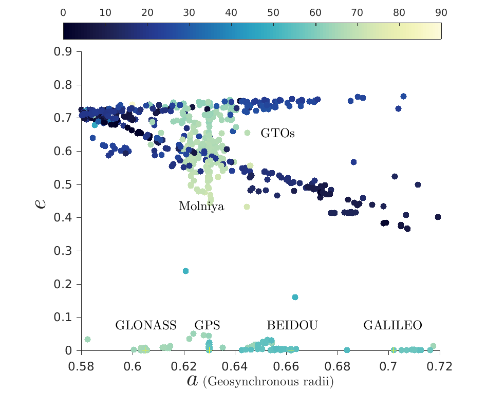
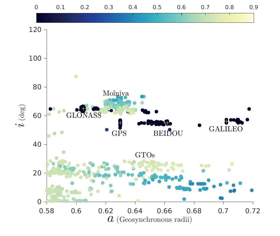
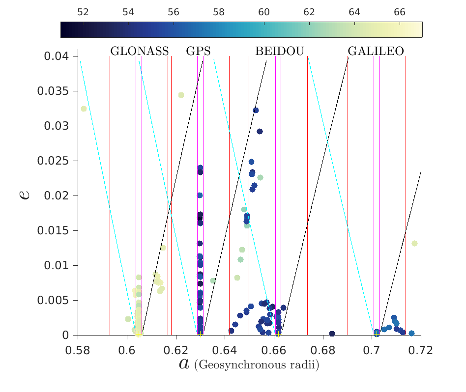
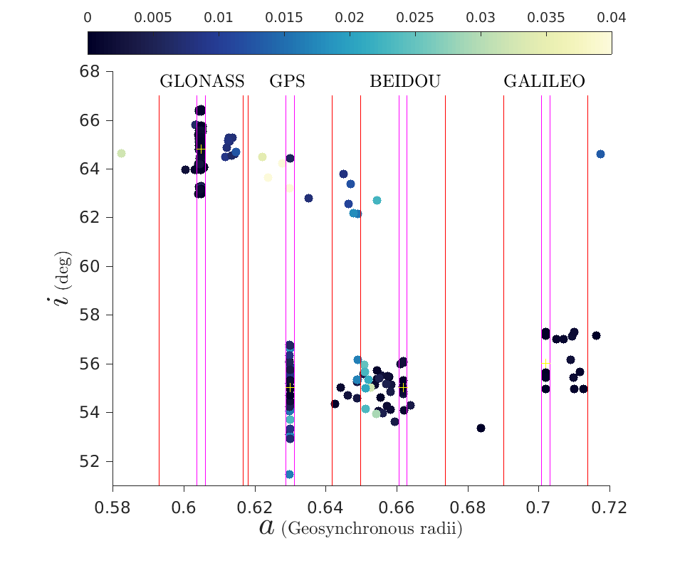
Figure 1: The cataloged resident space objects in the semi-major axis–eccentricity (left) and semi-major axis–inclination (right) space, where the colorbar corresponds to the “missing” of the three elements in each two-dimensional projection (dark blue corresponds to low values, while yellow indicates high values). The top figures correspond to $e\in\left[0,0.9\right]$, whereas the bottom figures focus around the GNSS orbital space. Vertical lines correspond to limits in $a$, $a_{nom}\pm 50$ km (magenta) and $a_{nom}\pm 500$ km (red), while slanted lines denote limits in apogee/perigee altitude, for each graveyard zone (see definition in the text). (Resident Space Object Catalog, www.space-track.org; assessed 25 Oct. 2016)

2.2 Set-up and dynamical model

One of the purposes of this study is to find reentry and graveyard orbits that could be useful in the design of EoL strategies. To this end, we perform “$200$yr-long” simulations over a large grid of initial conditions, as defined bellow. We use a dynamical model that accounts for the gravitational potential of Earth up to degree and order 2 (i.e., $J_{20}$, $J_{22}$), the Moon and Sun as perturbing bodies, and direct solar radiation pressure (SRP), using the “cannonball model” (McInnes, 1999). We do not include shadowing effects that we assume to be negligible far away from the LEO region. Atmospheric drag plays a major role in the evolution of low-altitude satellites. On the other hand, it is negligible in the MEO/GNSS region, as bodies with low to moderate eccentricities cannot reach low-enough altitudes, and hence we do not include it in our model.

For our numerical integrations, we use our SWIFT-SAT integrator, which is based on the mixed-variable symplectic integrator of Wisdom and Holman (1991), as included in the SWIFT package of Levison and Duncan (1994). SWIFT-SAT uses the full equations of motion and is suitable for dynamical studies of bodies with negligible mass, orbiting an oblate central body and perturbed by other massive bodies. In addition, SWIFT-SAT is able to incorporate weakly dissipative effects. We refer the reader to Rosengren et al. (2019) for a more in-depth discussion of SWIFT-SAT and particular validations that were performed to ensure effective performance.

In this study, we focus on a region of semi-major axes close to the GNSS. First, we adopt a wide grid of initial conditions in $a$, $e$ and $i$ (hereafter denoted as MEO-general), as shown in Table 1; it is actually more refined than the grid used in the “LEO-to-GEO” study presented in Rosengren et al. (2019). As the initial orbit orientation angles ($\Omega$ and $\omega$) also affect secular evolution, we chose to study $16$ different configurations. Finally, the initial mean anomaly was always set to $M=0$.

We are also interested in mapping the graveyard solutions around the nominal GNSS values of $a$, $e$ and $i$. We set the nominal eccentricity for all GNSS groups to $e_{nom}=10^{-4}$. We also set the nominal semi-major axis and inclination values for each GNSS group as shown in Table 2. We assume the “protected” region for each GNSS group to be within $\pm 50~{}$km from $a_{nom}$. Accordingly, we define the graveyard regions to be in the range $a\in\left[a_{nom}-500,a_{nom}-50\right]$ km (hereafter denoted as REGION I) and $a\in\left[a_{nom}+50,a_{nom}+500\right]$ km (hereafter denoted as REGION II). In addition to this, the perigee/apogee limiting altitudes of an acceptable graveyard solution should be such that they do not cross any neighboring protected region. According to this definition, graveyard orbits with $e>0.018$ do not exist. In Table 2, the limits for $a$, perigee (denoted as $q$) and apogee (denoted as $Q$) are shown and are also described graphically in the bottom panels of Fig. 1. Hence, an accepted graveyard solution should not violate any boundary during the whole 200 years of evolution. The grid of initial conditions used for our GNSS-graveyard study follows the above definitions, with a mesh of $da=5\cdot 10^{-4}a_{GEO}\simeq 20$ km and $de=5\cdot 10^{-4}$. We studied three values of initial inclination for each group, namely $i_{nom}$ and $i_{nom}\pm 0.5$, and we repeat the calculations for the same set of $\Omega$, $\omega$, and $M$ values as in our MEO-general study.

Both for the MEO-general study and in the GNSS-graveyard study, all computations were performed for two preselected epochs (JD 2458475.2433, denoted hereafter as “Epoch 2018”, and JD 2459021.78, hereafter “Epoch 2020”, see Rosengren et al. (2019)) and for two different values of $C_{R}A/m$; a typical one for spent upper stages and space debris (0.015 m²/kg) and an augmented one (1 m²/kg), assumed to represent a satellite equipped with a large sail (or, a smaller debris); the augmented $A/m$ value was used only in our MEO-general study. The time span for integration was $120$ yr (MEO-general) and $200$ yr (GNSS-graveyard) respectively, the time-step of integration was $dt=4\cdot 10^{-3}$ sidereal days, and our Earth reentry limit was set to $R_{E}+400$ km. In total, a set of $\sim$ 6 million initial conditions were propagated.

Table 1: Grids of initial conditions for the MEO-general study using SWIFT-SAT, for dynamical maps in $a-e$ phase space, as a function of $i$.

$a$ $(a_{GEO})$	$0.600-0.710$
$\Delta a$	$0.0025$
$e$	$0-0.88$
$\Delta e$	$0.02$
$i$ $(^{\circ})$	$0-90$
$\Delta i$ $(^{\circ})$	$2$
$\Delta\Omega$ (∘)	$\left\{0,90,180,270\right\}$
$\Delta\omega$ (∘)	$\left\{0,90,180,270\right\}$
$C_{R}(A/m)$ (m2/kg)	$\left\{0.015,1\right\}$

Table 2: Grids of initial conditions for the GNSS-graveyard study using SWIFT-SAT, for dynamical maps in $a-e$ phase space, as a function of $i$. Values of $\Omega$, and $\omega$ were set as shown in Table 1, and $C_{R}(A/m)=0.015$ m²/kg.

	GLONASS	GPS
$a_{nom}$ $\left(\right.$km $\left.\left|~{}a_{GEO}\right)\right.$	$25509.64~{}|~{}0.605$	$26561.18~{}|~{}0.630$
$i_{nom}$ $(^{\circ})$	$64.8$	$55$
REGION I	$a\in\left[a_{GLO}-500,a_{GLO}-50\right]$ km	$a\in\left[a_{GPS}-500,a_{GPS}-50\right]$ km
	$q>0$	$q\geq a_{GLO}+50$km
	$Q\leq a_{GLO}-50$km	$Q\leq a_{GPS}-50$km
REGION II	$a\in\left[a_{GLO}+50,a_{GLO}+500\right]$ km	$a\in\left[a_{GPS}+50,a_{GPS}+500\right]$ km
	$q\geq a_{GLO}+50$km	$q\geq a_{GPS}+50$km
	$Q\leq a_{GPS}-50$km	$Q\leq a_{BEI}-50$km
	BEIDOU	GALILEO
$a_{nom}$ $(km~{}|~{}a_{GEO})$	$27906.14~{}|~{}0.662$	$29601.31~{}|~{}0.702$
$i_{nom}$ $(^{\circ})$	$55$	$56$
REGION I	$a\in\left[a_{BEI}-500,a_{BEI}-50\right]$ km	$a\in\left[a_{GAL}-500,a_{GAL}-50\right]$ km
	$q\geq a_{GPS}+50$km	$q\geq a_{BEI}+50$km
	$Q\leq a_{BEI}-50$km	$Q\leq a_{GAL}-50$km
REGION II	$a\in\left[a_{BEI}+50,a_{BEI}+500\right]$ km	$a\in\left[a_{GAL}+50,a_{GAL}+500\right]$ km
	$q\geq a_{BEI}+50$km	$q\geq a_{GAL}+50$km
	$Q\leq a_{GAL}-50$km	$Q\leq a_{GAL}+2500$km

3 Dynamical Atlas

3.1 MEO-general study

The results of our numerical simulations performed for the MEO region are presented here in the form of dynamical maps. In each 2-D map, the initial grid in $\left(a,e\right)$ for a specific initial inclination, $i$, a given set of orientation angles, epoch and $C_{R}A/m$ value is presented. Color-coded is the dynamical lifetime of a trajectory (i.e., the time until it reaches our reentry limit in $q$) or the eccentricity indicator $De=(e_{max}-e_{0})/(e_{c}-e_{0})$. This quantity has the property of varying between 0 and 1 (in the region $e<e_{c}$) and is a direct measure of the eccentricity variation offered by the dynamics, relative what is needed to achieve atmospheric reentry (Gkolias et al., 2016). Hence, $De\rightarrow 1$ means that an initial eccentricity, $e_{0}$, grows to a maximum value, $e_{max}$, that is greater or equal to the critical value for reentry, $e_{c}$.

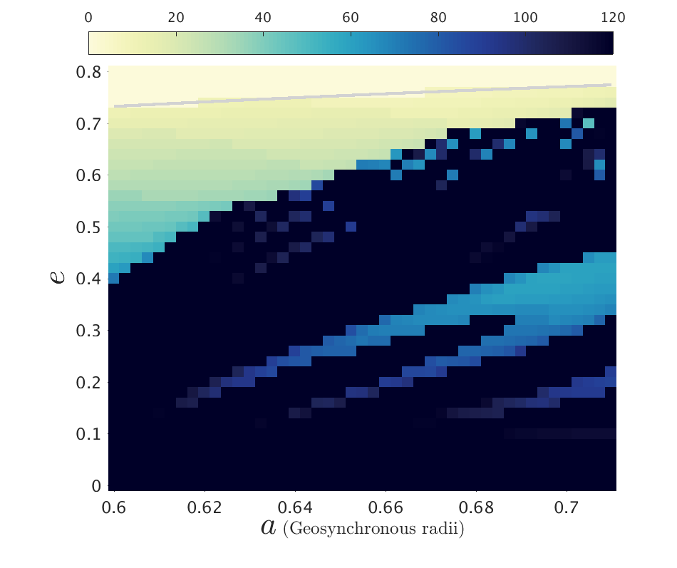
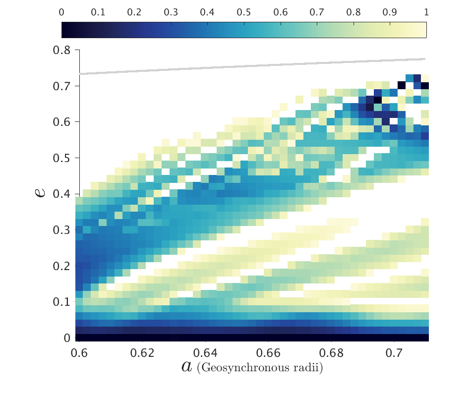
(a) $\bm{\Delta}\bm{\Omega}={\bf 180^{\circ}}$, $\bm{\Delta}\bm{\omega}={\bf 0}$

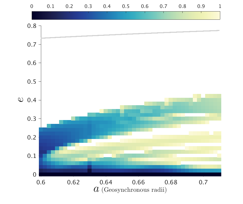
(b) $\bm{\Delta}\bm{\Omega}={\bf 180^{\circ}}$, $\bm{\Delta}\bm{\omega}={\bf 90^{\circ}}$

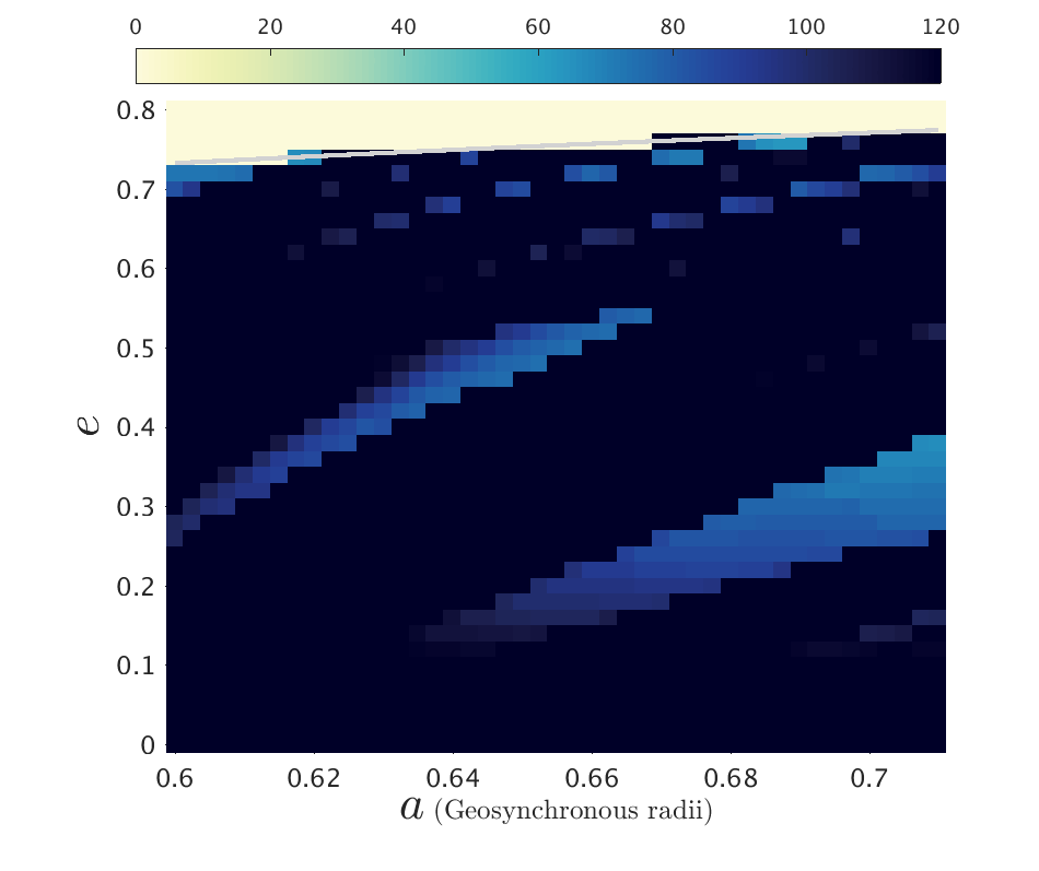
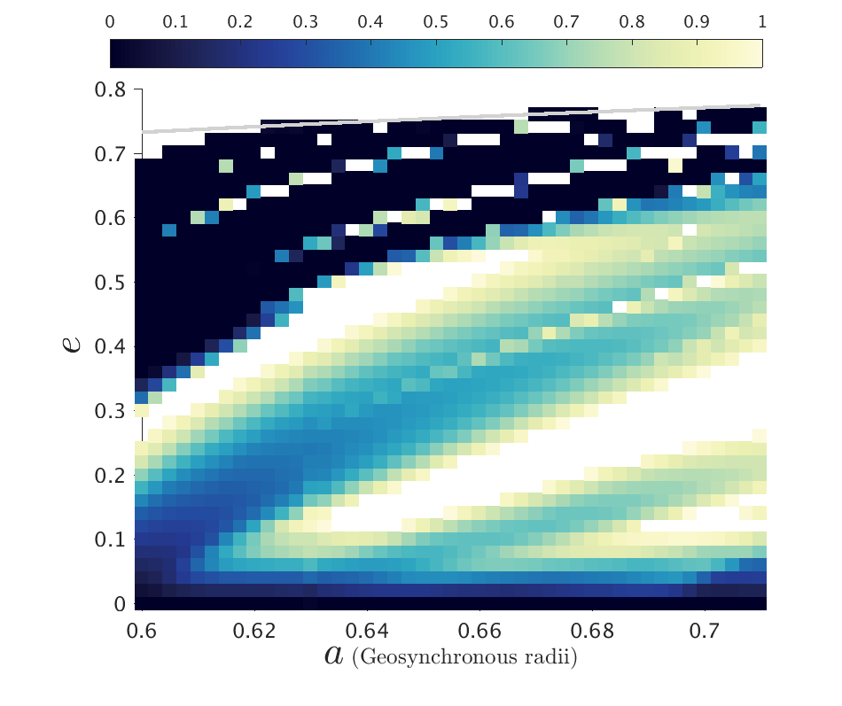
(c) $\bm{\Delta}\bm{\Omega}={\bf 270^{\circ}}$, $\bm{\Delta}\bm{\omega}={\bf 0}$

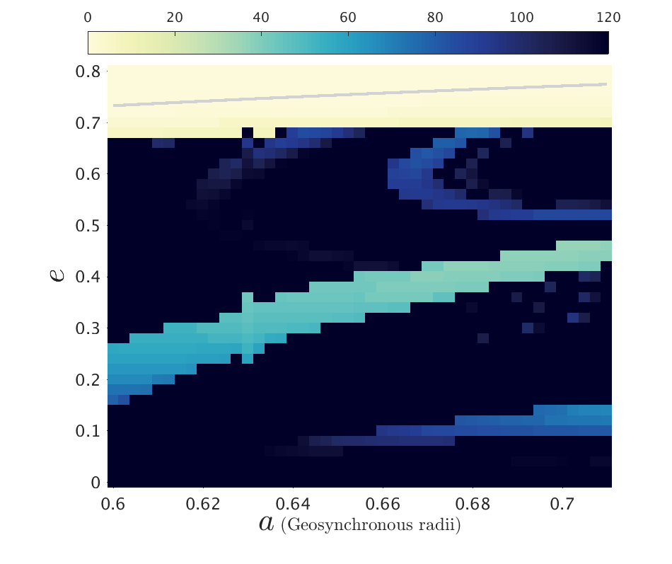
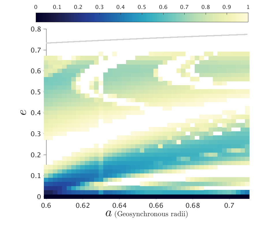
(d) $\bm{\Delta}\bm{\Omega}={\bf 270^{\circ}}$, $\bm{\Delta}\bm{\omega}={\bf 90^{\circ}}$

Figure 3: Lifetime and $De$ maps of the MEO-general phase space for $\bm{i_{o}}={\bf 56^{\circ}}$, for Epoch 2018, and for $C_{R}A/m=0.015$ m²/kg. The colorbar for the lifetime maps is from 0 to 120 years and that of the $De$ maps is from 0 to 1.

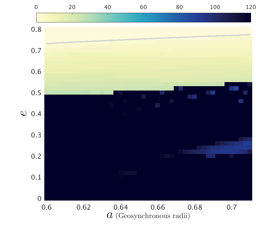
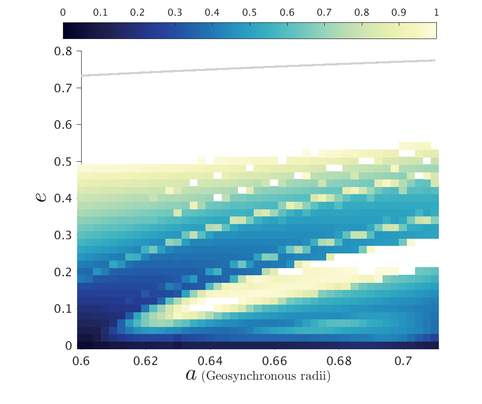
(a) $\bm{\Delta}\bm{\Omega}={\bf 0}$, $\bm{\Delta}\bm{\omega}={\bf 0}$

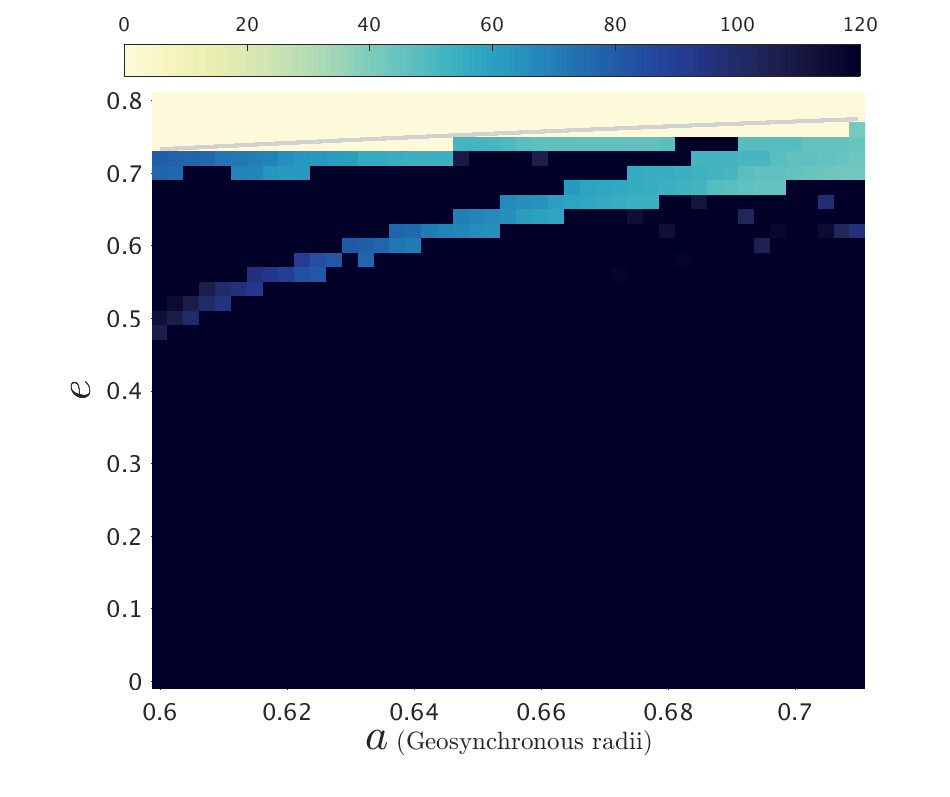
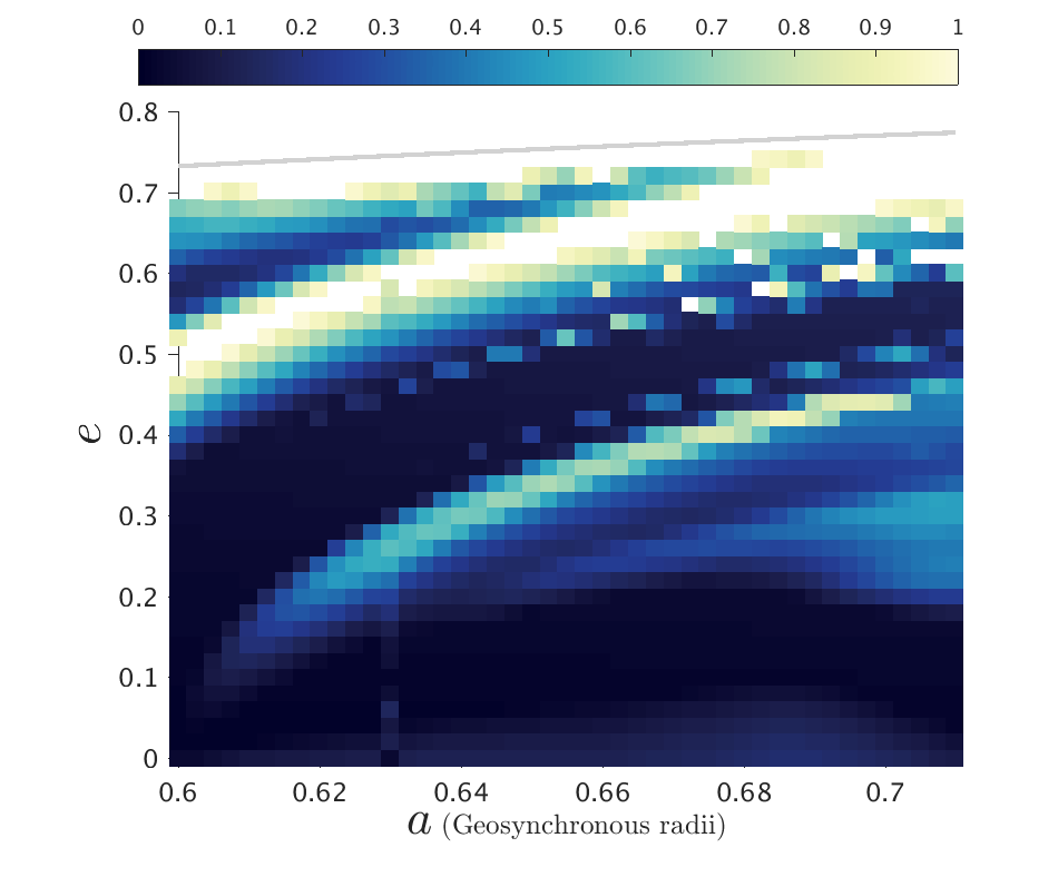
(b) $\bm{\Delta}\bm{\Omega}={\bf 0}$, $\bm{\Delta}\bm{\omega}={\bf 90^{\circ}}$

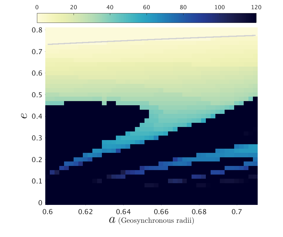
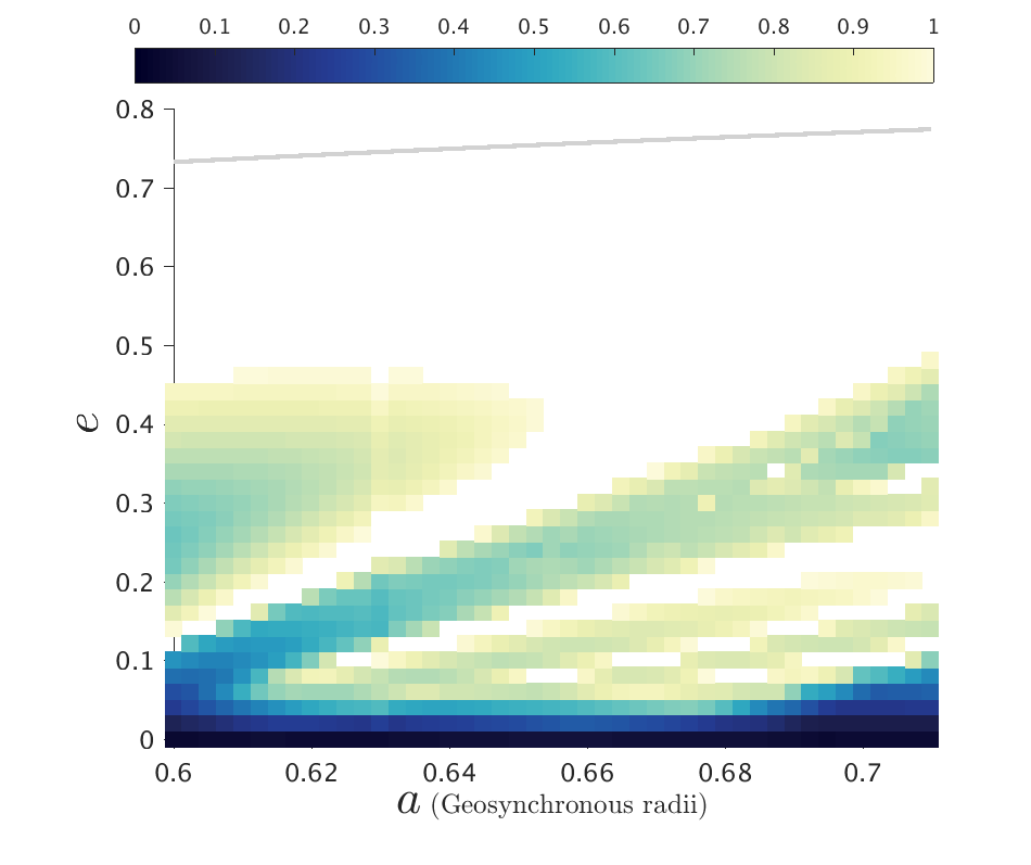
(c) $\bm{\Delta}\bm{\Omega}={\bf 90^{\circ}}$, $\bm{\Delta}\bm{\omega}={\bf 0}$

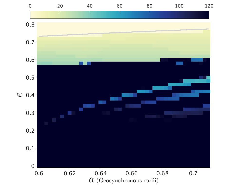
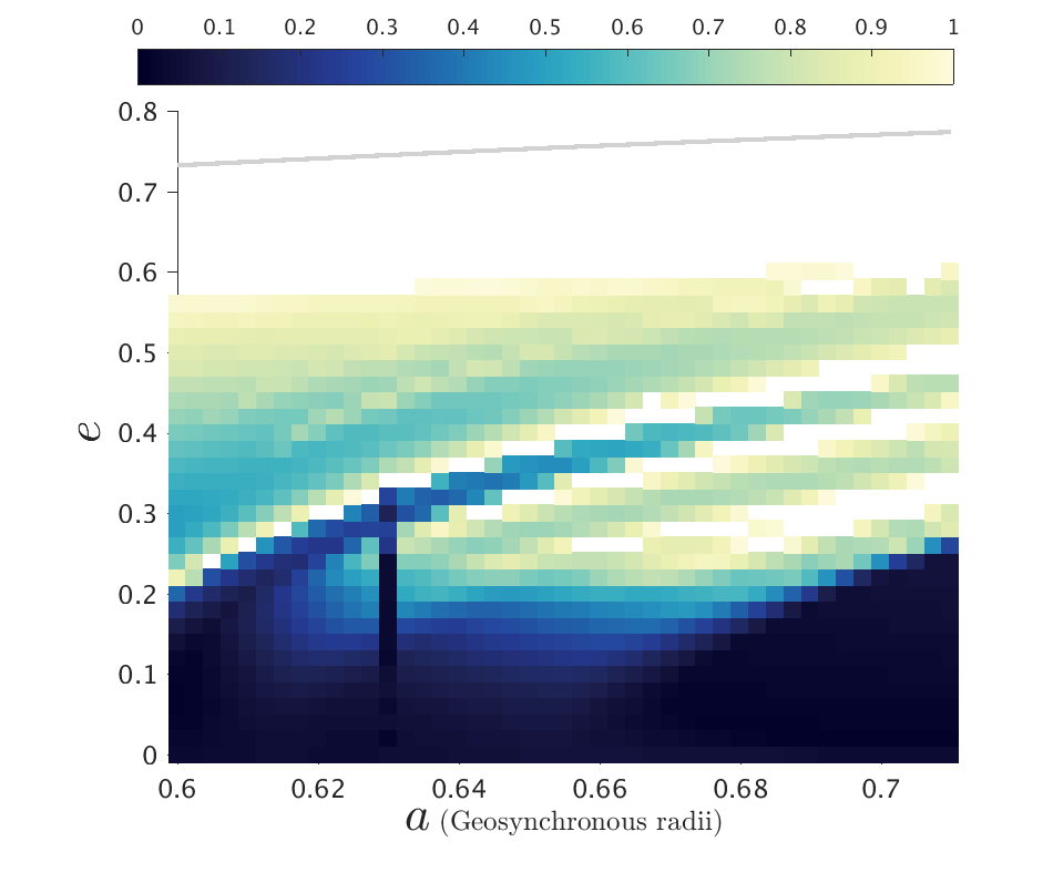
(d) $\bm{\Delta}\bm{\Omega}={\bf 90^{\circ}}$, $\bm{\Delta}\bm{\omega}={\bf 90^{\circ}}$

Figure 4: Lifetime and $De$ maps of the MEO-general phase space for $\bm{i_{o}}={\bf 56^{\circ}}$, for Epoch 2018, and for $C_{R}A/m=1$ m²/kg. The colorbar for the lifetime maps is from 0 to 120 years and that of the $De$ maps is from 0 to 1.

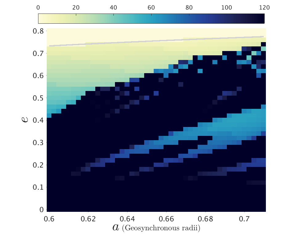
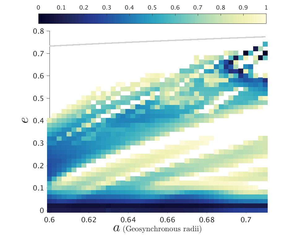
(a) $\bm{\Delta}\bm{\Omega}={\bf 180^{\circ}}$, $\bm{\Delta}\bm{\omega}={\bf 0}$

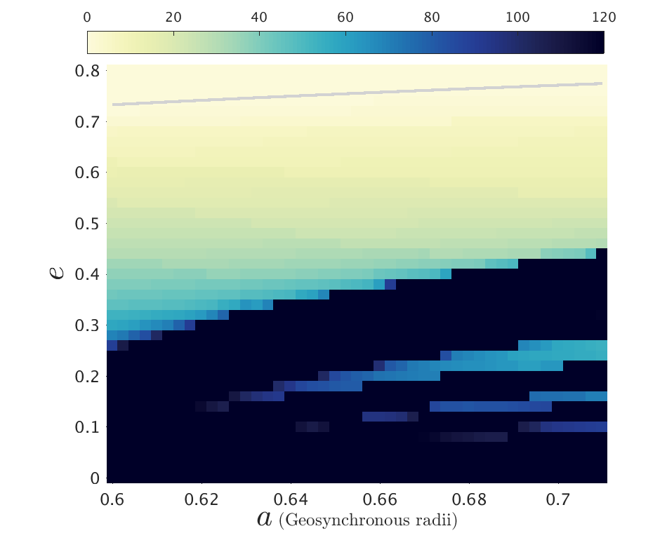
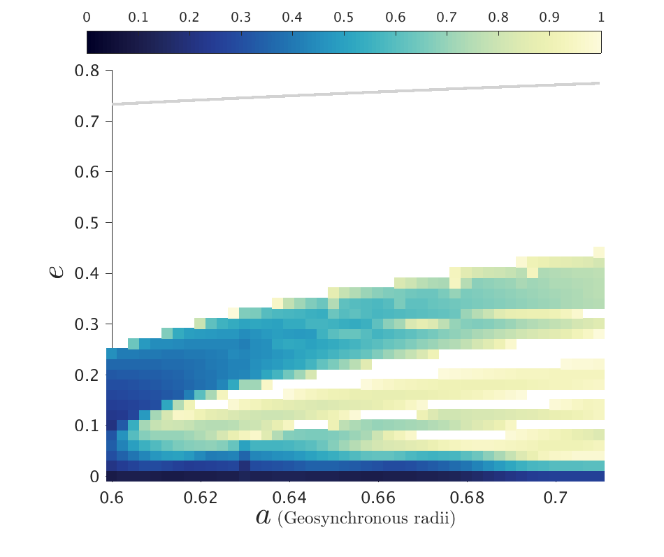
(b) $\bm{\Delta}\bm{\Omega}={\bf 180^{\circ}}$, $\bm{\Delta}\bm{\omega}={\bf 90^{\circ}}$

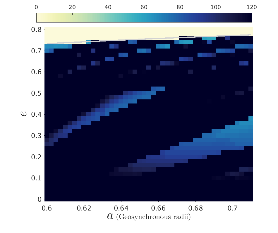
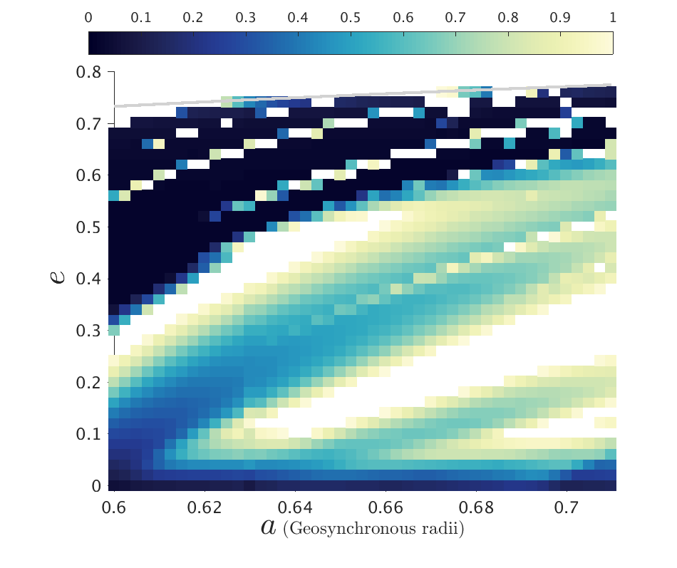
(c) $\bm{\Delta}\bm{\Omega}={\bf 270^{\circ}}$, $\bm{\Delta}\bm{\omega}={\bf 0}$

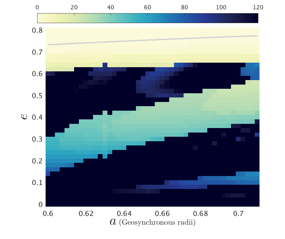
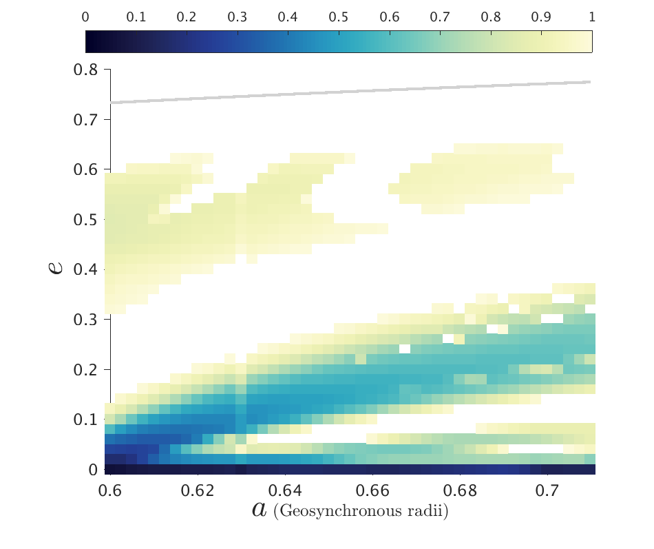
(d) $\bm{\Delta}\bm{\Omega}={\bf 270^{\circ}}$, $\bm{\Delta}\bm{\omega}={\bf 90^{\circ}}$

Figure 5: Lifetime and $De$ maps of the MEO-general phase space for $\bm{i_{o}}={\bf 56^{\circ}}$, for Epoch 2018, and for $C_{R}A/m=1$ m²/kg. The colorbar for the lifetime maps is from 0 to 120 years and that of the $De$ maps is from 0 to 1.

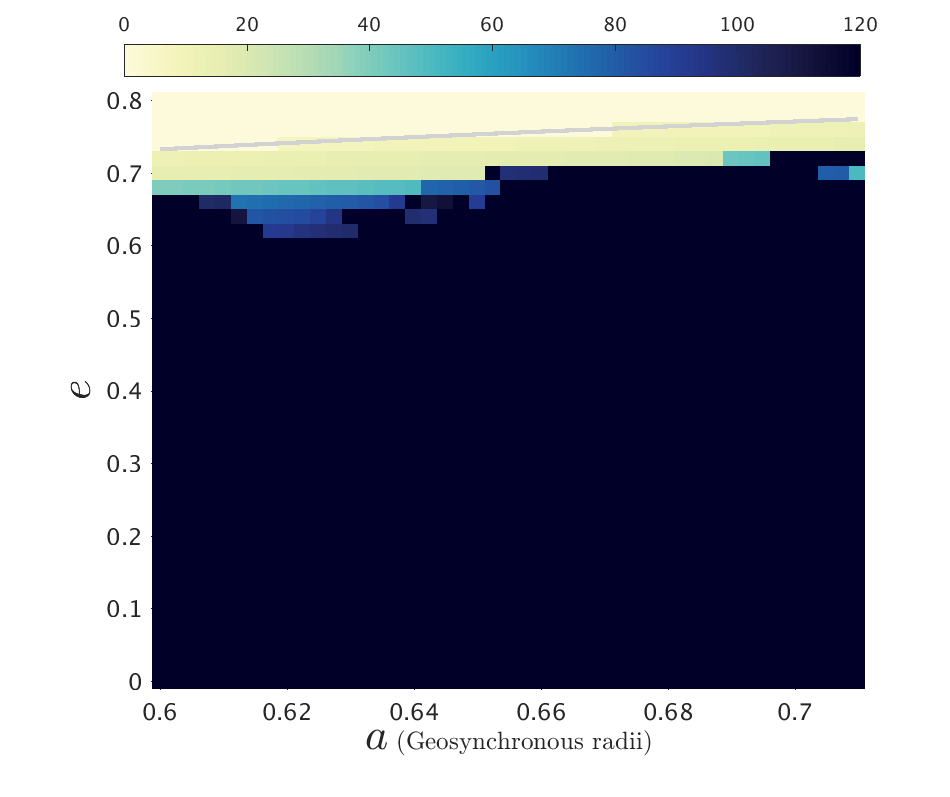
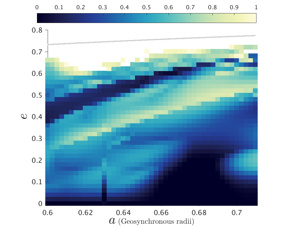
(a) $\bm{\Delta}\bm{\Omega}={\bf 0}$, $\bm{\Delta}\bm{\omega}={\bf 0}$

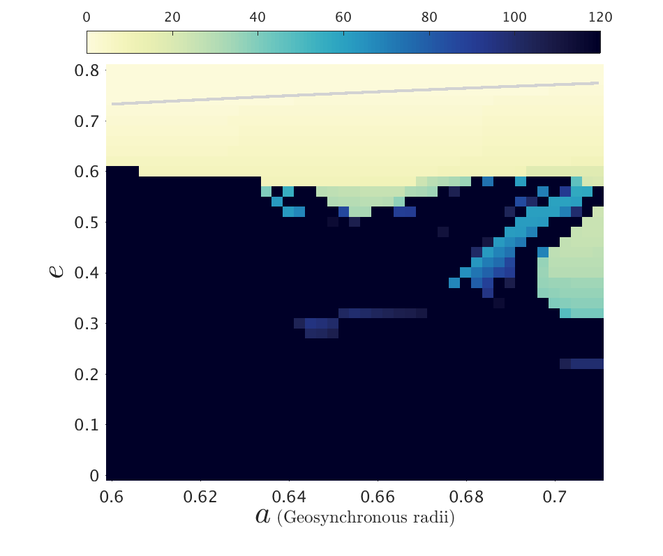
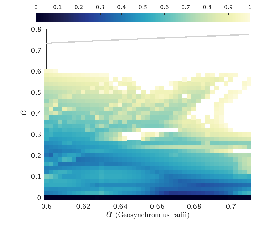
(b) $\bm{\Delta}\bm{\Omega}={\bf 0}$, $\bm{\Delta}\bm{\omega}={\bf 90^{\circ}}$

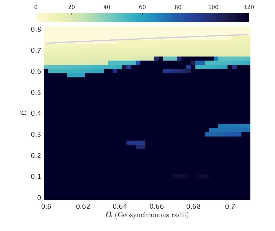
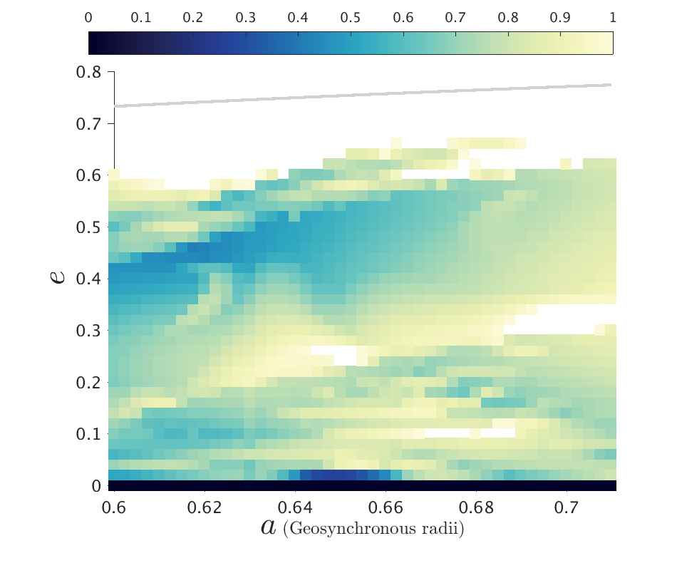
(c) $\bm{\Delta}\bm{\Omega}={\bf 90^{\circ}}$, $\bm{\Delta}\bm{\omega}={\bf 0}$

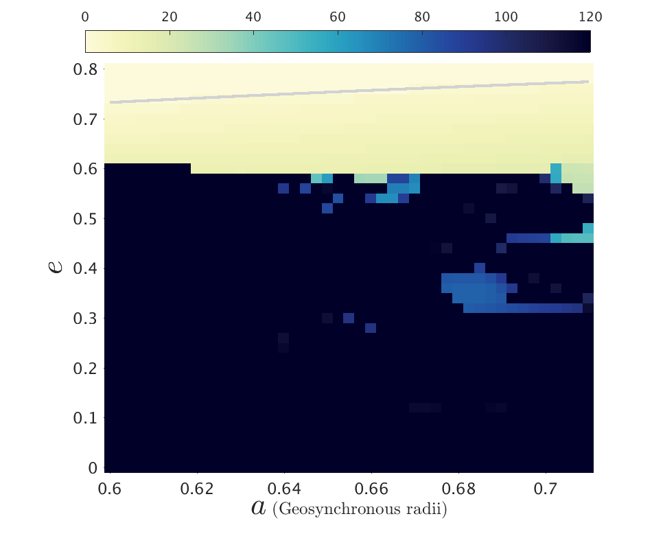
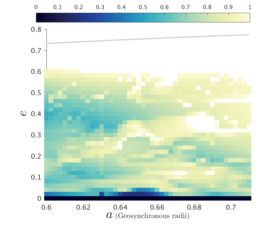
(d) $\bm{\Delta}\bm{\Omega}={\bf 90^{\circ}}$, $\bm{\Delta}\bm{\omega}={\bf 90^{\circ}}$

Figure 6: Lifetime and $De$ maps of the MEO-general phase space for $\bm{i_{o}}={\bf 64^{\circ}}$, for Epoch 2018, and for $C_{R}A/m=0.015$ m²/kg. The colorbar for the lifetime maps is from 0 to 120 years and that of the $De$ maps is from 0 to 1.

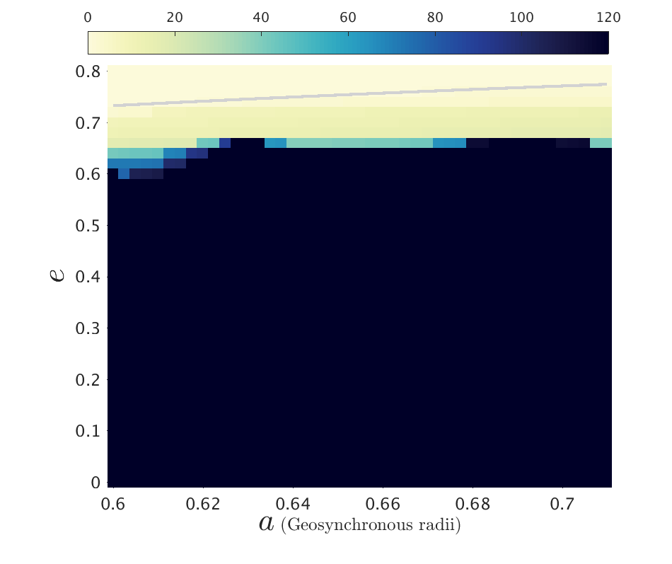
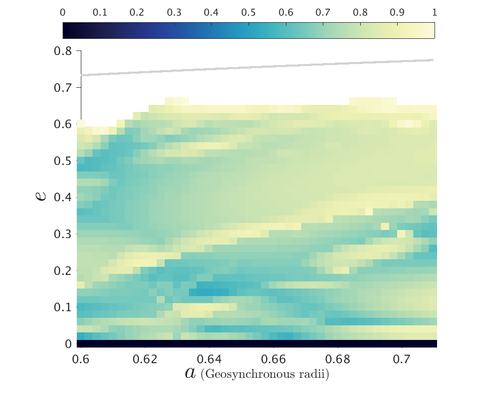
(a) $\bm{\Delta}\bm{\Omega}={\bf 180^{\circ}}$, $\bm{\Delta}\bm{\omega}={\bf 0}$

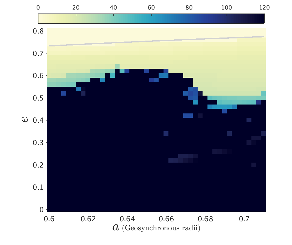
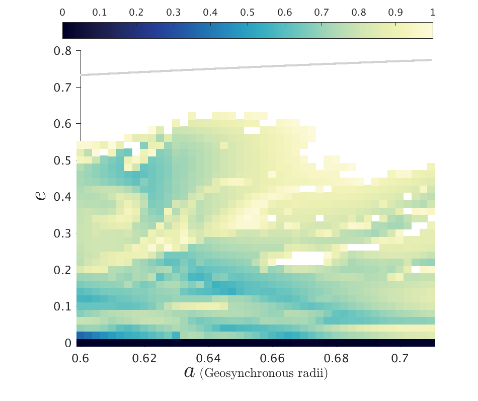
(b) $\bm{\Delta}\bm{\Omega}={\bf 180^{\circ}}$, $\bm{\Delta}\bm{\omega}={\bf 90^{\circ}}$

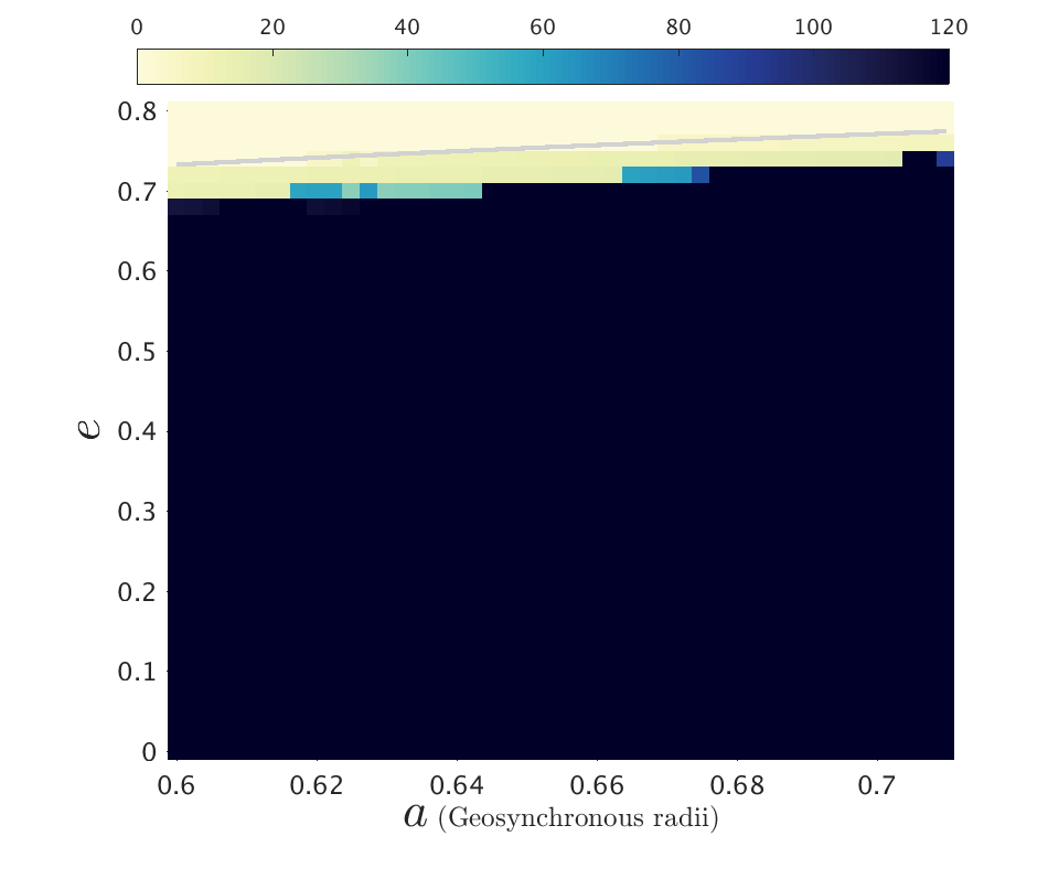
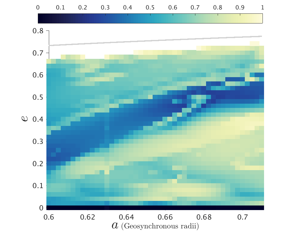
(c) $\bm{\Delta}\bm{\Omega}={\bf 270^{\circ}}$, $\bm{\Delta}\bm{\omega}={\bf 0}$

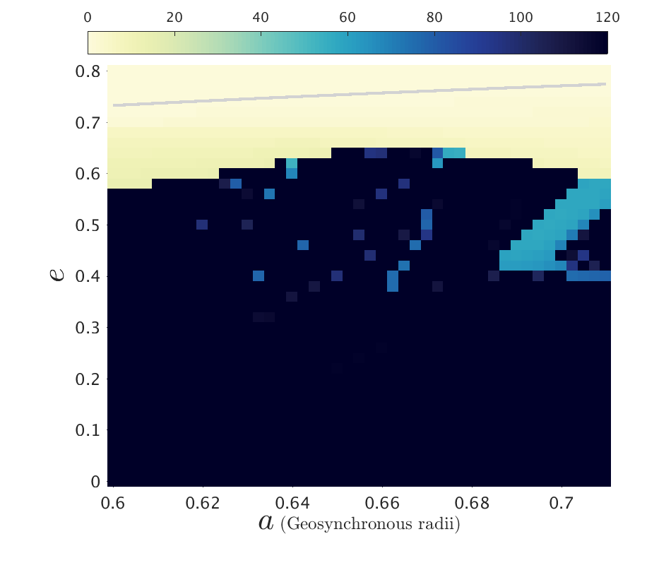
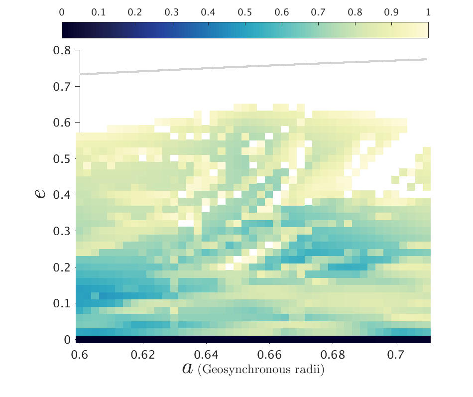
(d) $\bm{\Delta}\bm{\Omega}={\bf 270^{\circ}}$, $\bm{\Delta}\bm{\omega}={\bf 90^{\circ}}$

Figure 7: Lifetime and $De$ maps of the MEO-general phase space for $\bm{i_{o}}={\bf 64^{\circ}}$, for Epoch 2018, and for $C_{R}A/m=0.015$ m²/kg. The colorbar for the lifetime maps is from 0 to 120 years and that of the $De$ maps is from 0 to 1.

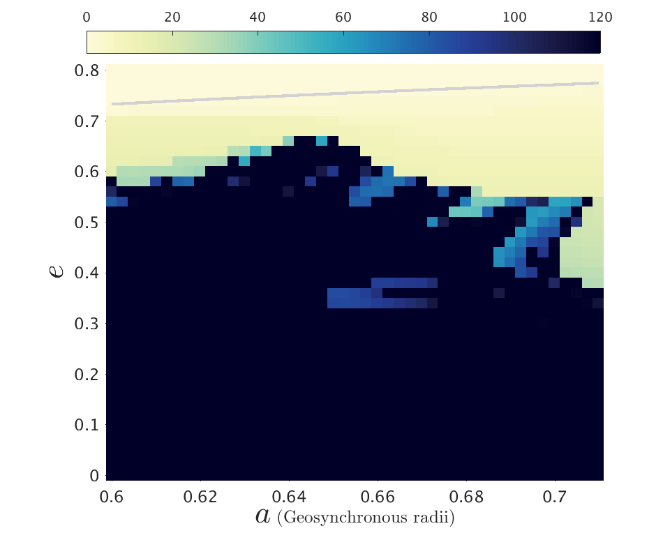
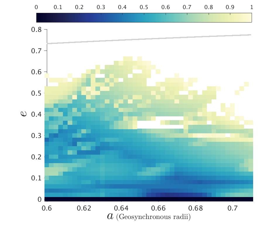
(a) $\bm{\Delta}\bm{\Omega}={\bf 0}$, $\bm{\Delta}\bm{\omega}={\bf 0}$

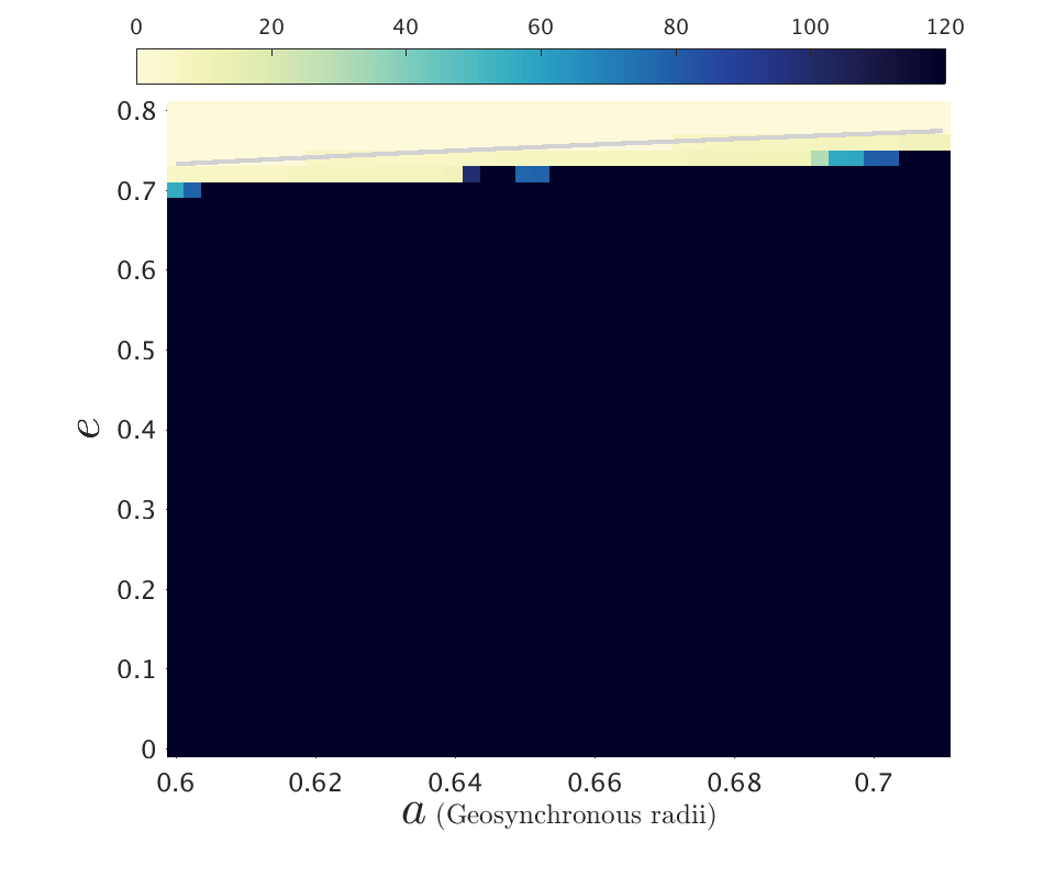
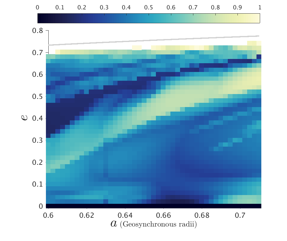
(b) $\bm{\Delta}\bm{\Omega}={\bf 0}$, $\bm{\Delta}\bm{\omega}={\bf 90^{\circ}}$

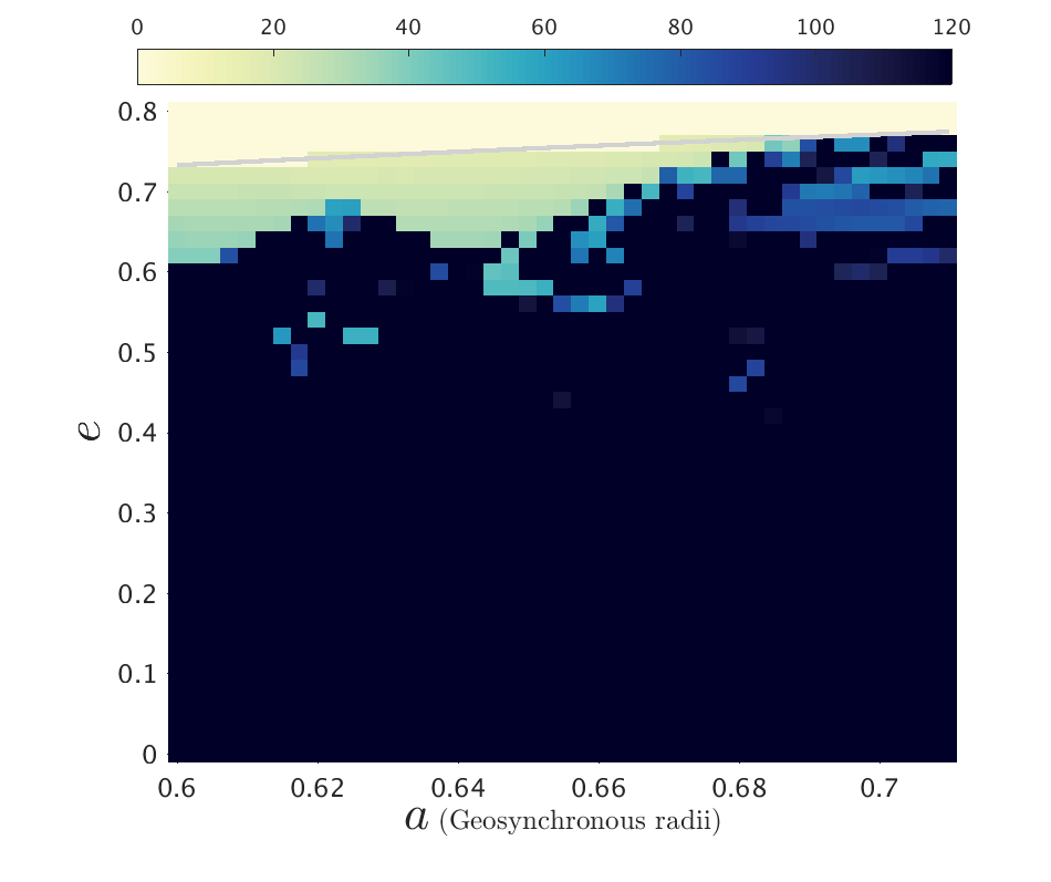
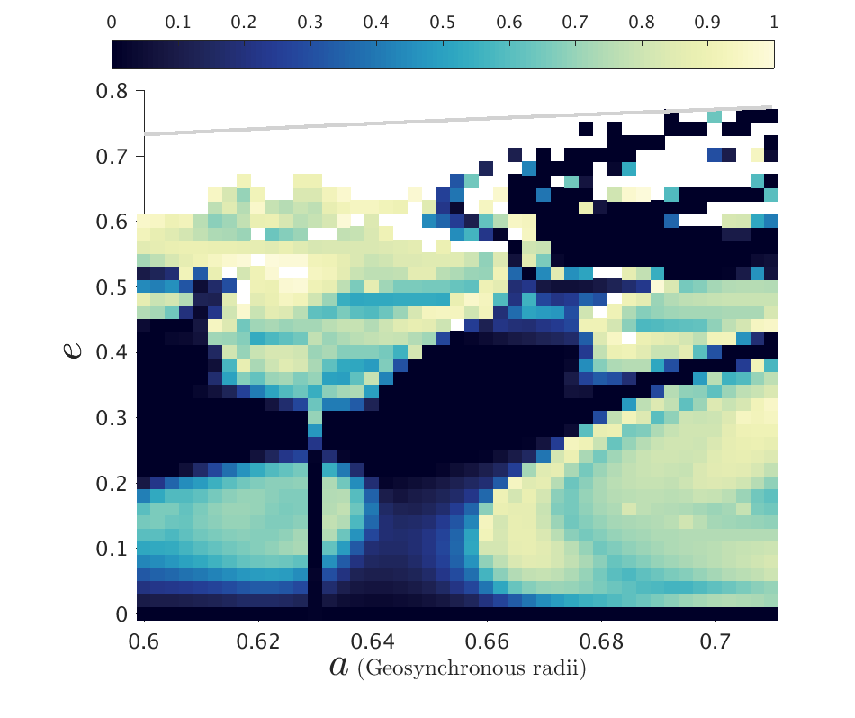
(c) $\bm{\Delta}\bm{\Omega}={\bf 90^{\circ}}$, $\bm{\Delta}\bm{\omega}={\bf 0}$

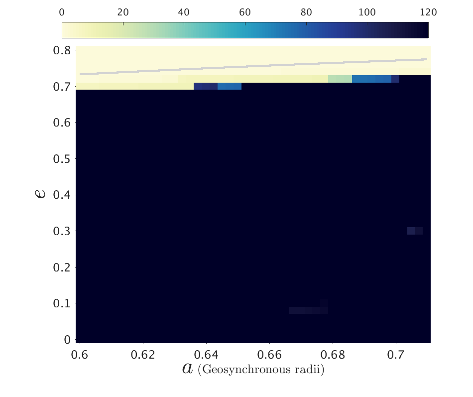
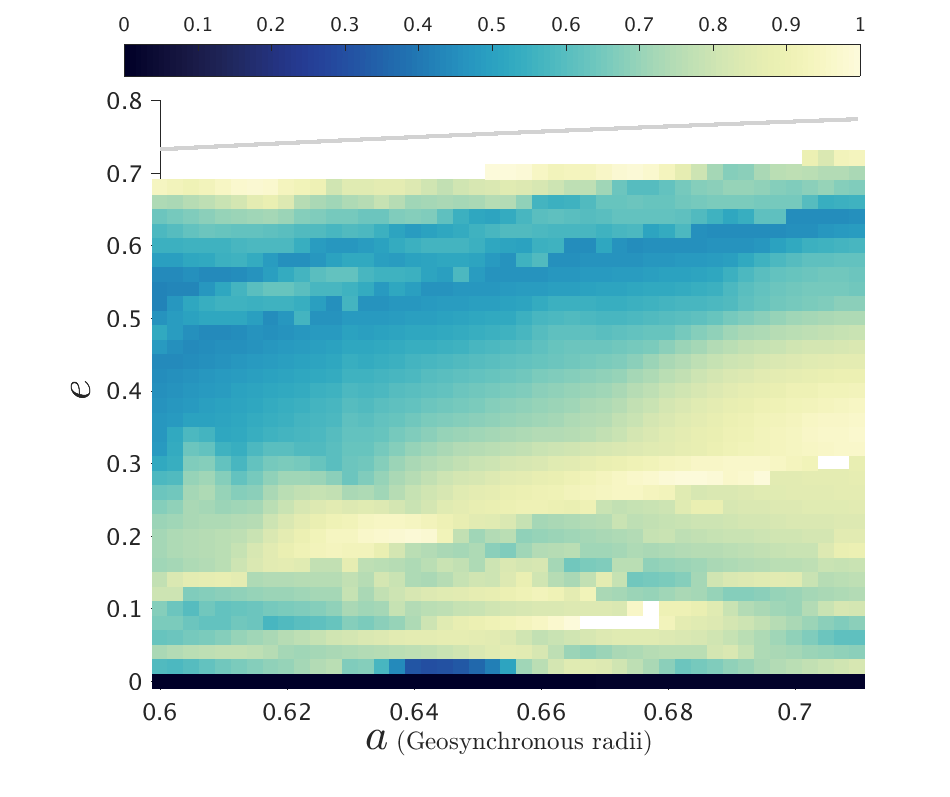
(d) $\bm{\Delta}\bm{\Omega}={\bf 90^{\circ}}$, $\bm{\Delta}\bm{\omega}={\bf 90^{\circ}}$

Figure 8: Lifetime and $De$ maps of the MEO-general phase space for $\bm{i_{o}}={\bf 64^{\circ}}$, for Epoch 2020, and for $C_{R}A/m=0.015$ m²/kg. The colorbar for the lifetime maps is from 0 to 120 years and that of the $De$ maps is from 0 to 1.

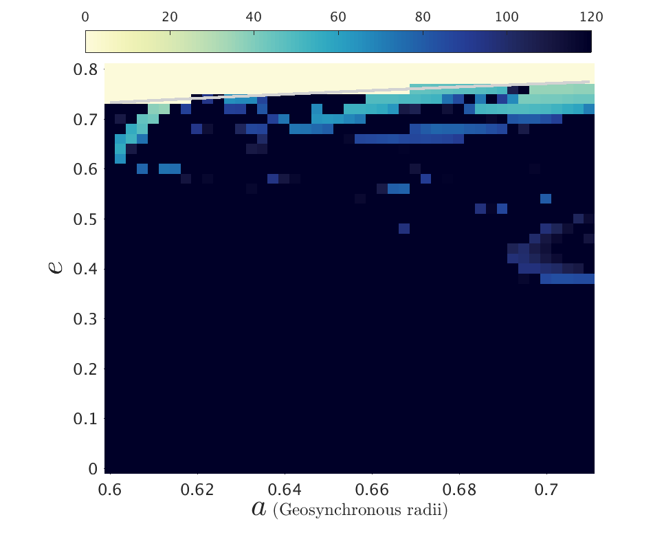
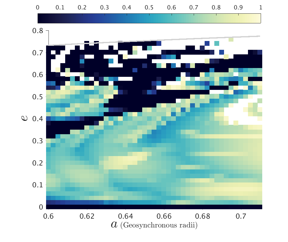
(a) $\bm{\Delta}\bm{\Omega}={\bf 180^{\circ}}$, $\bm{\Delta}\bm{\omega}={\bf 0}$

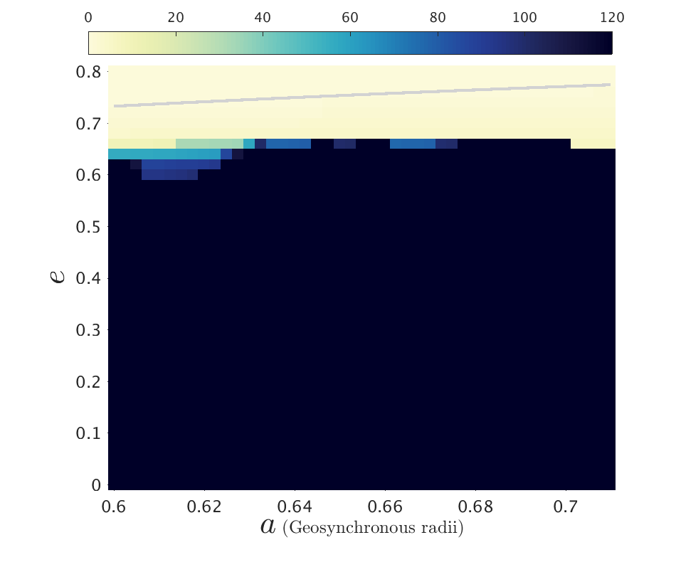
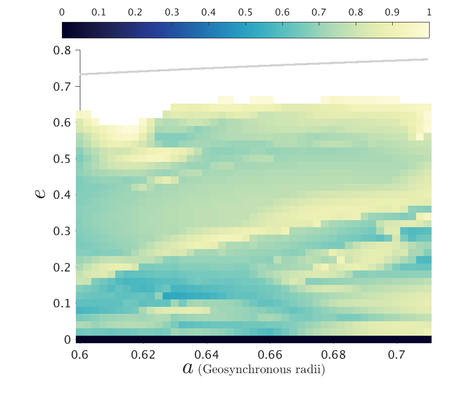
(b) $\bm{\Delta}\bm{\Omega}={\bf 180^{\circ}}$, $\bm{\Delta}\bm{\omega}={\bf 90^{\circ}}$

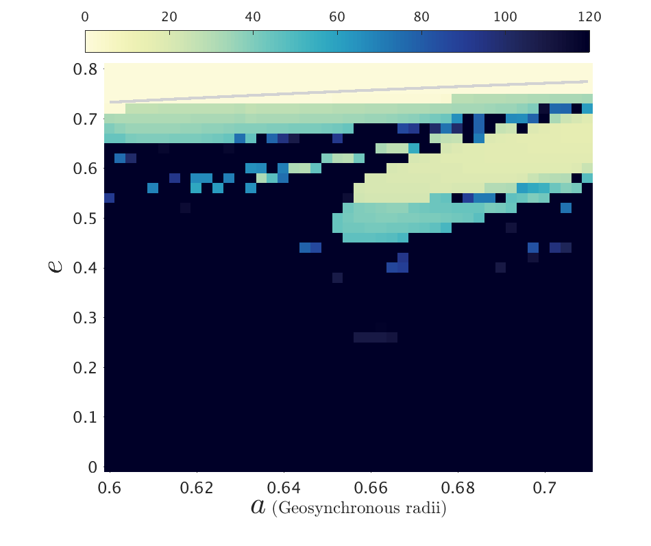
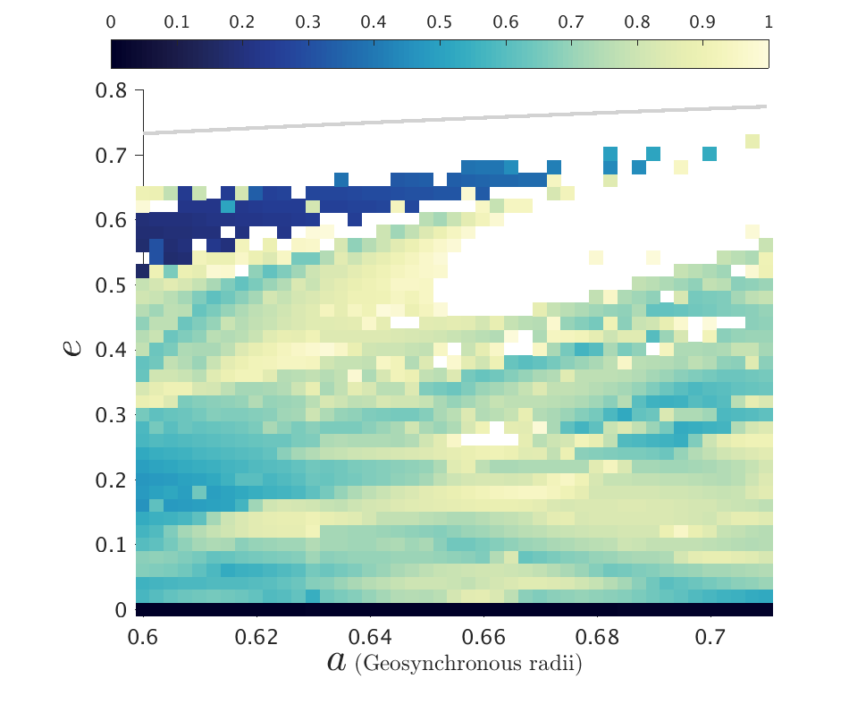
(c) $\bm{\Delta}\bm{\Omega}={\bf 270^{\circ}}$, $\bm{\Delta}\bm{\omega}={\bf 0}$

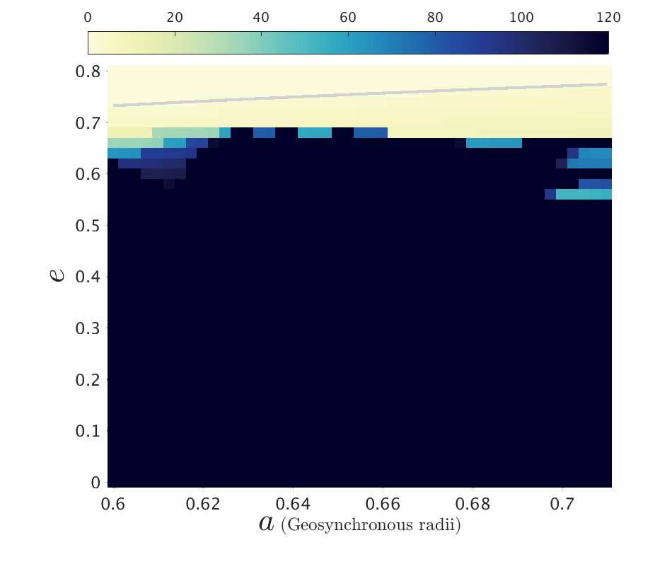
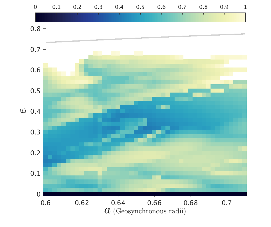
(d) $\bm{\Delta}\bm{\Omega}={\bf 270^{\circ}}$, $\bm{\Delta}\bm{\omega}={\bf 90^{\circ}}$

Figure 9: Lifetime and $De$ maps of the MEO-general phase space for $\bm{i_{o}}={\bf 64^{\circ}}$, for Epoch 2020, and for $C_{R}A/m=0.015$ m²/kg. The colorbar for the lifetime maps is from 0 to 120 years and that of the $De$ maps is from 0 to 1.

Figures 2-9 show a subset of our results for $i_{o}=56^{\circ}$ and $64^{\circ}$. In the A, a subset of our results for various inclinations is also shown. The results of our complete atlas, for all inclinations, both epochs and both $C_{R}A/m$ values, can be found at the ReDSHIFT website . Figure 10 shows (on the left) the frequency $f_{r}$ of reentry solutions with $q>R_{E}+400$km, over the whole initial grid, and (on the right), the mean dynamical lifetime $\tilde{t}_{r}$ of the reentry population (solid lines) and the minimum lifetime of the reentry population with $e_{0}<0.3$ (dashed lines), as functions of the initial inclination, $i_{o}$.

For low to moderate inclinations (up to $\sim 40^{\circ}$) as well as for high inclinations ($>\sim 80^{\circ}$), the structure of the maps is quite smooth and very few reentry solutions can be found, even after $120$ yr. The typical values are $f_{r}<0.04$ and $\tilde{t}_{r}>115$ yr. Note that, at such inclinations, there is practically no strong secular resonances, and hence no strong instabilities (Rosengren et al., 2019). For inclinations between $\sim 40^{\circ}$ and $\sim 80^{\circ}$ the structure is more complicated. Figure 10 reveals three distinct inclination regions where $f_{r}$ shows relative maxima, at $i_{o}=$46^∘, 56^∘, and 68^∘. Note that these curves show ‘angle-averaged’ results (i.e., all values of $\Omega$ and $\omega$ are combined for each $i_{o}$). Numerous studies in the past decade or so (Chao, 2000; Jenkin and Gick, 2005; Rossi, 2008; Daquin et al., 2015; Rosengren et al., 2015; Alessi et al., 2016; Celletti and Galeş, 2016; Gkolias et al., 2016; Rosengren et al., 2017) have highlighted the importance of lunisolar secular resonances near GNSS inclinations. Resonances lead to eccentricity growth (decrease of perigee distance), whereas resonance overlapping introduces chaos in their orbits, on top of any regular, secular excitation. Those phenomena can lead a nearly circular GNSS orbit to reentry on centennial timescales. Our results suggest that $f_{r}\left(i_{o}\right)$ and $\tilde{t}_{r}\left(i_{o}\right)$ are roughly independent on $C_{R}A/m$. This is strongly indicative of the absence of dynamical influence of solar (semi-secular) resonances, i.e. a minimal effect of SRP. Moreover, the curves also seem to be roughly the same, independent of the initial epoch chosen. Again, these are ’angle- averaged’ results, and this indicates that the initial choice of $\Omega$ and $\omega$ is (on average) not important on the long run. However, note that the effect of lunisolar resonances on $e$ and $i$ do depend on the initial values orientation of these two angles, but also on a ‘third angle’ (i.e. epoch), namely the lunar (ecliptic) node $\left(\Omega_{M}\right)$. The two initial epochs chosen in this study are relatively close to each other, and hence $\Omega_{M}$ does not differ by much $\left(\sim 30^{\circ}\right)$; in equatorial coordinates, $\Omega_{M,eq}$ is almost the same in both epochs. Hence, even if – as shown in our dynamical maps – the results can differ substantially for the two epochs, we cannot really conclude that Figure 10 is ’epoch-invariant’. In fact, integrating for more (and more distant) epochs could reveal a near- periodic variation of $f_{r}$ and/or $\tilde{t}_{r}$, but we expect that the central values of the peaks will be roughly preserved, as they represent the location (in $i$) of known lunisolar resonances. Another feature, noticeable in the $De$ maps, is a thin, vertical band at the location of the 2:1 commensurability with the Earth’s rotation rate ($a\approx 0.63~{}a_{GEO}$), where the variation of $De$ may appear as ‘discontinuous’ with respect to the neighboring values of $a$. This resonance leads to coupled oscillations in $a$ and $e$, but is quite narrow in $a$ so that, at our grid resolution, it has the width of only once cell. Depending on the choice of orientation angles, the eccentricities of resonant particles will remain low, if they are close to the stable equilibrium point of the resoannce, characterised by a value of the resonant angle $\sigma=\lambda-2\lambda_{E}+\varpi\approx 0$, or will increase significantly, if $\sigma\approx\pi$ (the unstable fixed point of the resonance). However, the overall dynamical structure of the neighborhood is not severely affected.

According to our results, for inclinations near the nominal values for the the GPS, BEIDOU and GALILEO groups and for low $C_{R}A/m$, $\sim 35\%$ of our initial conditions can re-enter, with a mean dynamical lifetime of $\sim 90$ yr. There is, though, a strong dependence on the orientation of the secular angles. Nevertheless, reentry orbits with lifetimes $\sim 40$ yr can occur even for eccentricities smaller than $\sim 0.15$. For inclinations near the GLONASS nominal value, only $\sim 15\%$ of the initial conditions reenter, with a mean dynamical lifetime of $\sim 90$ yr. Despite the fact that the reentry particles with initial $e<0.3$ and dynamical lifetimes of $\sim 30$ yr exist, disposal dynamical hatches appear generally at higher eccentricities, which could make it much harder to actually use as disposal strategy. Note that $De$ for non-escaping orbits that are found close to reentry hatches is $De>0.8$, which indicates a significant increase of eccentricity and, hence, possible reentry at times somehow longer than $120$ years. When an augmented $C_{R}A/m$ is used, the reentry regions widen and the lifetimes decrease by a few years on average at all inclinations, but the overall structure of the maps is preserved.

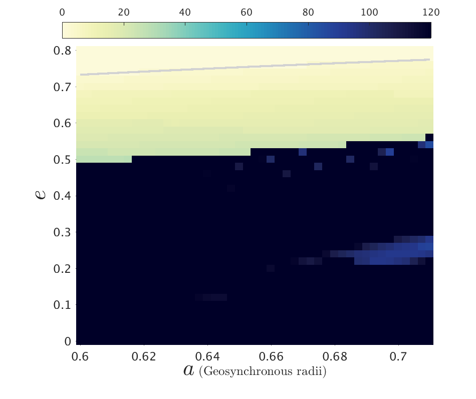
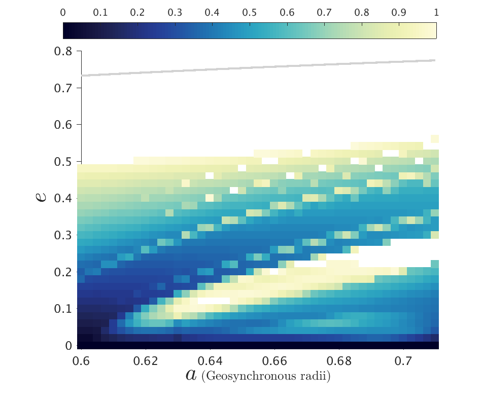
(a) $\bm{\Delta}\bm{\Omega}={\bf 0}$, $\bm{\Delta}\bm{\omega}={\bf 0}$

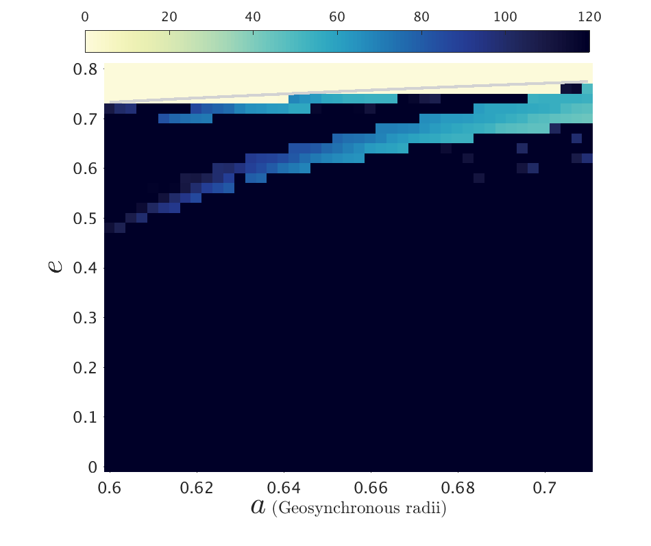
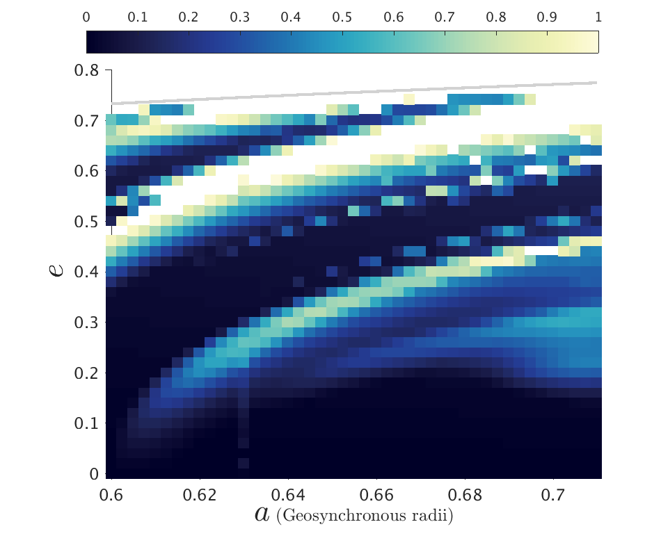
(b) $\bm{\Delta}\bm{\Omega}={\bf 0}$, $\bm{\Delta}\bm{\omega}={\bf 90^{\circ}}$

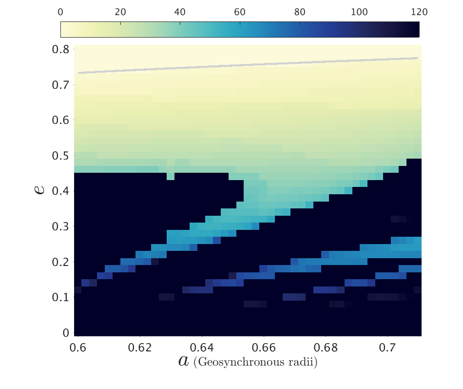
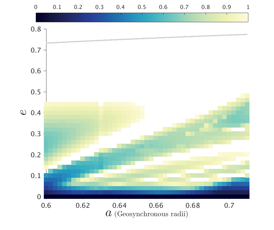
(c) $\bm{\Delta}\bm{\Omega}={\bf 90^{\circ}}$, $\bm{\Delta}\bm{\omega}={\bf 0}$

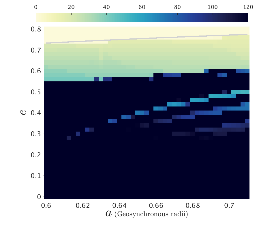
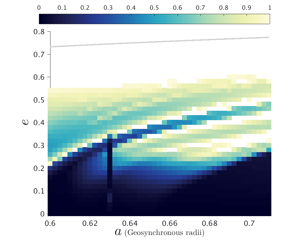
(d) $\bm{\Delta}\bm{\Omega}={\bf 90^{\circ}}$, $\bm{\Delta}\bm{\omega}={\bf 90^{\circ}}$

Figure 2: Lifetime and $De$ maps of the MEO-general phase space for $\bm{i_{o}}={\bf 56^{\circ}}$, for Epoch 2018, and for $C_{R}A/m=0.015$ m²/kg. The colorbar for the lifetime maps is from 0 to 120 years and that of the $De$ maps is from 0 to 1.

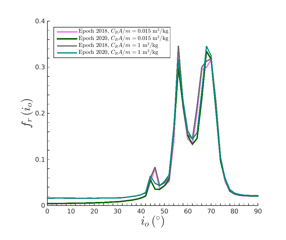
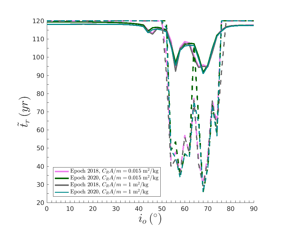
Figure 10: Frequency, $f_{r}$, (left) and mean dynamical lifetime, $\tilde{t}_{r}$, (right) of the reentry population with $q>R_{E}+400$km, as function of initial inclination (see text for details on their calculation). Solid and dashed lines in $i_{o}-\tilde{t}_{r}$ diagram denote the mean dynamical lifetime of the entire reentry population and the minimum dynamical lifetime of the reentry population with initial $e\leq 0.3$, respectively. Different colors denote different initial epoch and $C_{R}A/m$; as it is indicated by the legend.

3.2 GNSS-graveyard study

This part of our study was performed assuming $C_{R}A/m=0.015$ m²/kg only. The grid of initial conditions that remain within the defined graveyard regions for a timespan of $200$ yr is presented in each dynamical map. Again, each $\left(a,e\right)$ map corresponds to a given set of $\left(\Omega,\omega\right)$, epoch and $i$ value. Color-coded is the maximum eccentricity that the orbit reaches during the 200 years of evolution.

Figures 11-12 show a subset of our results; more results can be found in B. The number of test-orbits that remain in the defined graveyard regions for $200$ yr depends on the initial secular angle configuration and epoch. It is obvious from the dynamical maps that eccentricity of surviving graveyards does not increase more than $\sim 0.02$; otherwise the orbit would violate our definition of graveyard. However, the structure of the maps is not entirely smooth. Table 3 shows the mean values of the fraction of the initial population that constitute acceptable graveyards over all combinations of $\left(\Omega,\omega\right)$ studied. Overall, $\sim 20-40\%$ of the initial test population constitute acceptable graveyards. Most of the particles with initial $e<0.001$ have survived for $200$ yr time-span, which is in consistent with the results shown in Radtke et al. (2015).

Table 3: Percentage of the initial population that remains within the defined graveyard region for $200$ yr. Mean values, $m_{i}$, for $i_{nom}$, and $i_{nom}\pm 0.5$ over the chosen set of $\left(\Omega,\omega\right)$ configurations.

	$m_{i_{nom}-0.5^{\circ}}$	$m_{i_{nom}}$	$m_{i_{nom}+0.5^{\circ}}$
GLONASS	$3.83$	$20.80$	$40.79$
GPS	$30.78$	$34.21$	$36.27$
BEIDOU	$20.74$	$25.49$	$27.67$
GALILEO	$20.78$	$31.76$	$35.02$

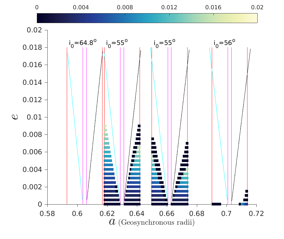
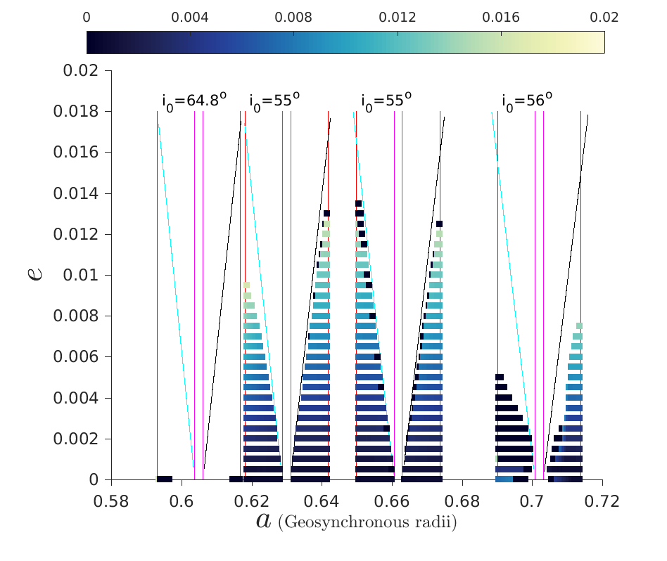
(a) $\bm{\Delta}\bm{\Omega}={\bf 0}$, $\bm{\Delta}\bm{\omega}={\bf 0}$

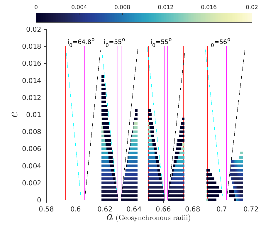
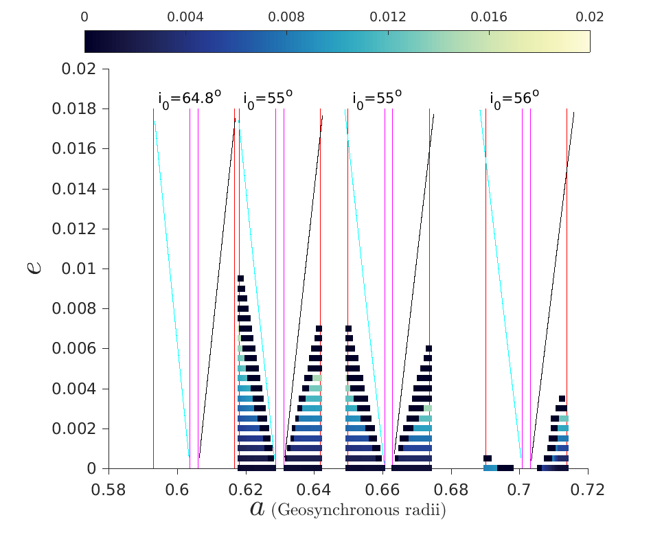
(b) $\bm{\Delta}\bm{\Omega}={\bf 0}$, $\bm{\Delta}\bm{\omega}={\bf 90^{\circ}}$

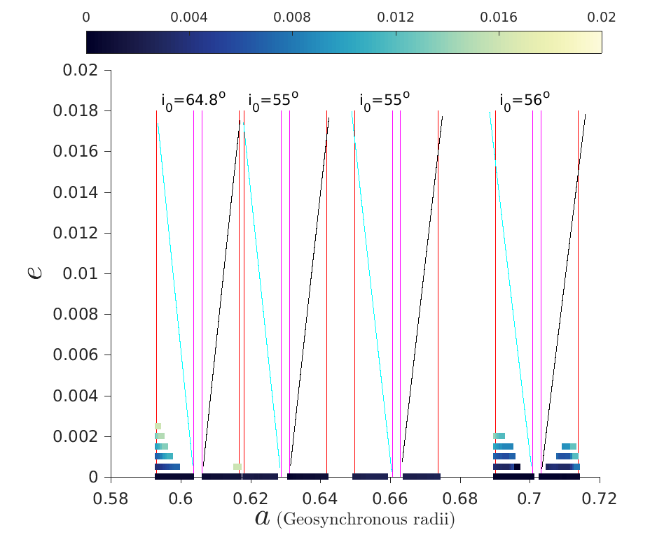
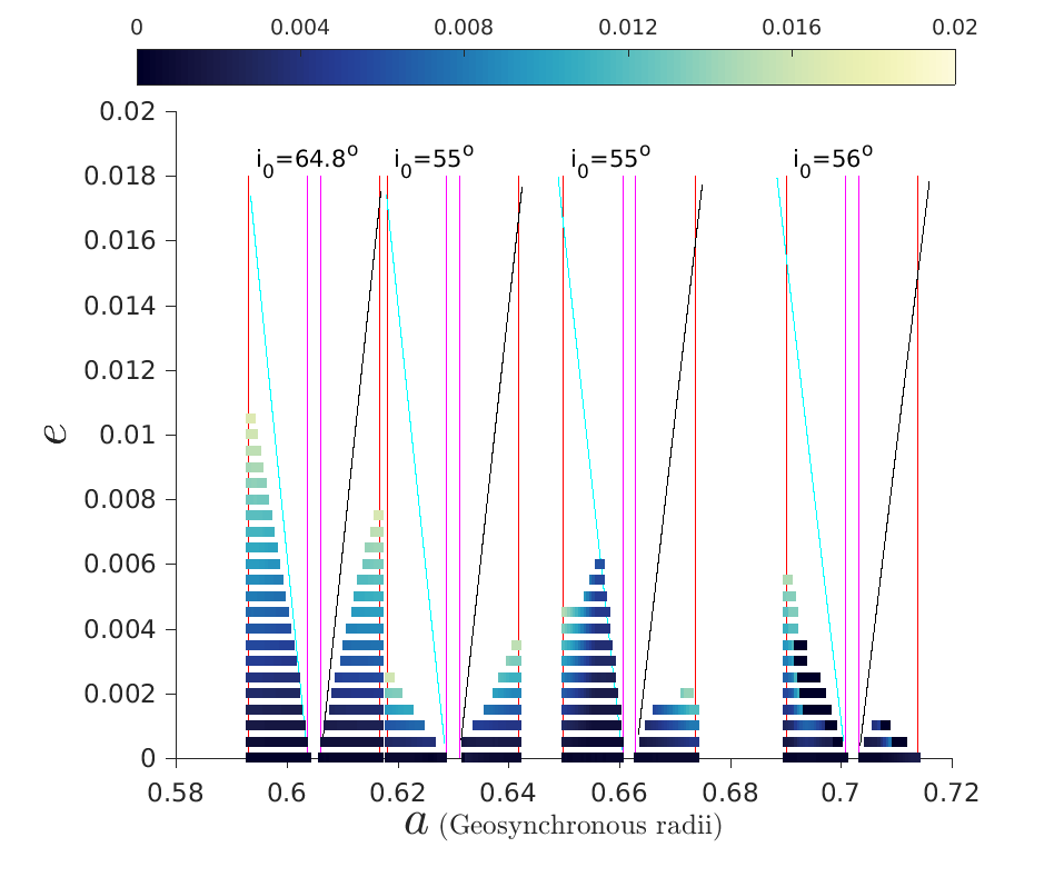
(c) $\bm{\Delta}\bm{\Omega}={\bf 90^{\circ}}$, $\bm{\Delta}\bm{\omega}={\bf 0}$

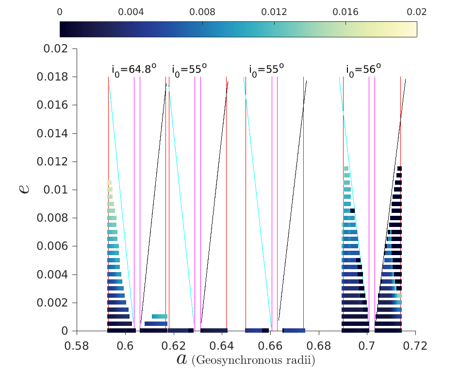
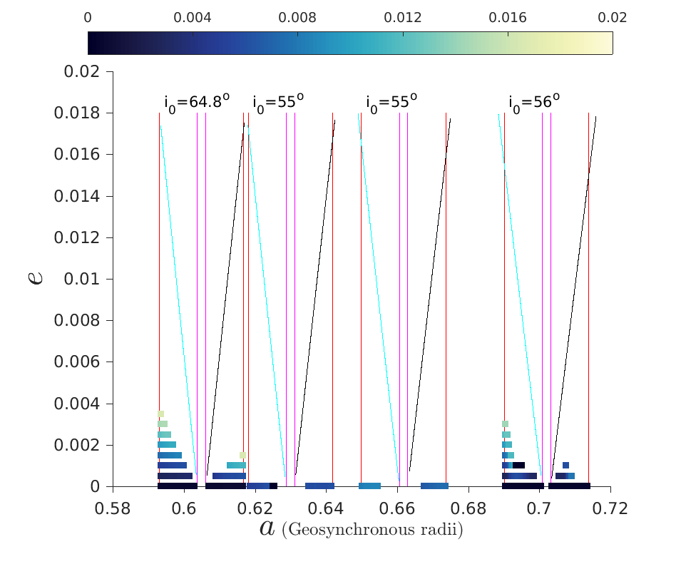
(d) $\bm{\Delta}\bm{\Omega}={\bf 90^{\circ}}$, $\bm{\Delta}\bm{\omega}={\bf 90^{\circ}}$

Figure 11: Maximum eccentricity maps of the GNSS-graveyard phase space for $\bm{i_{o}}={\bf i_{nom}}$, for Epoch 2018 (left) and Epoch 2020 (right), and for $C_{R}A/m=0.015$ m²/kg. $i_{nom}=64.8^{\circ}$ for GLONASS, $55^{\circ}$ for GPS and BEIDOU, and $56^{\circ}$ for GALILEO. The colorbar for maximum eccentricity maps is from 0 to 0.02.

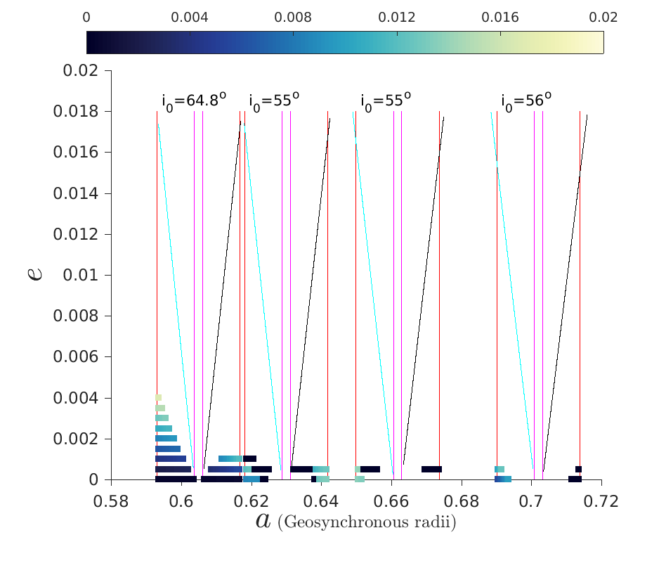
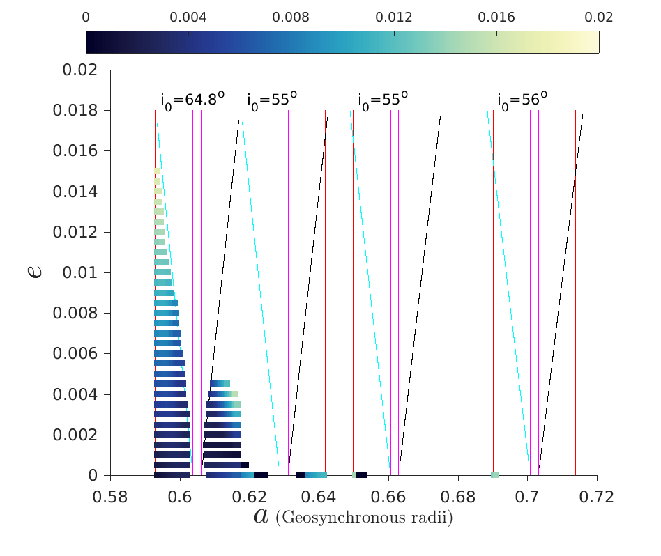
(a) $\bm{\Delta}\bm{\Omega}={\bf 180^{\circ}}$, $\bm{\Delta}\bm{\omega}={\bf 0}$

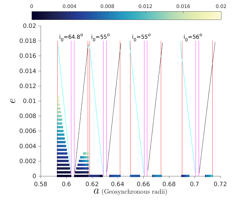
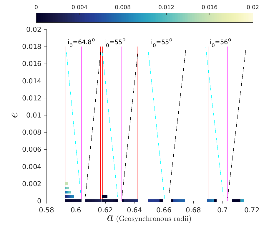
(b) $\bm{\Delta}\bm{\Omega}={\bf 180^{\circ}}$, $\bm{\Delta}\bm{\omega}={\bf 90^{\circ}}$

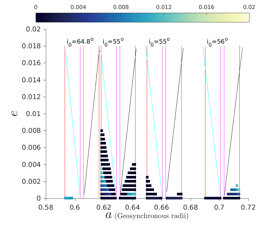
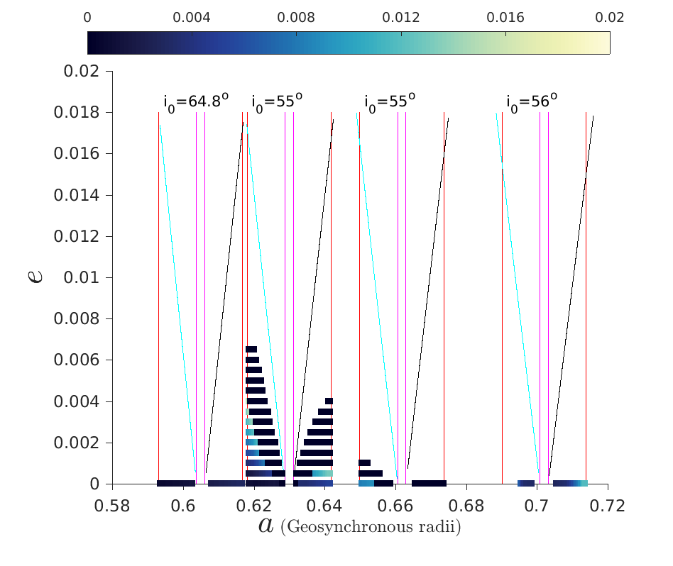
(c) $\bm{\Delta}\bm{\Omega}={\bf 270^{\circ}}$, $\bm{\Delta}\bm{\omega}={\bf 0}$

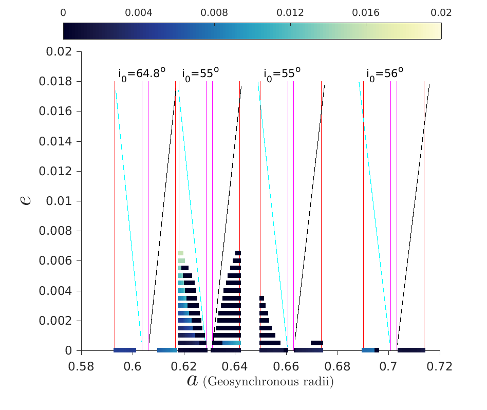
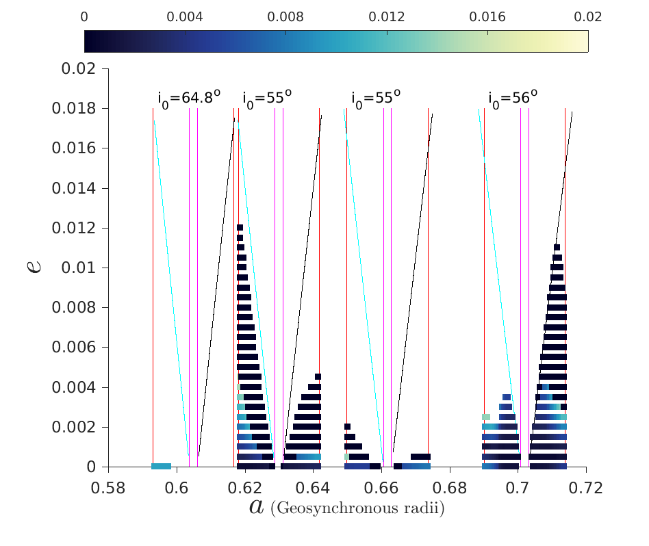
(d) $\bm{\Delta}\bm{\Omega}={\bf 270^{\circ}}$, $\bm{\Delta}\bm{\omega}={\bf 90^{\circ}}$

Figure 12: Maximum eccentricity maps of the GNSS-graveyard phase space for $\bm{i_{o}}={\bf i_{nom}}$, for Epoch 2018 (left) and Epoch 2020 (right), and for $C_{R}A/m=0.015$ m²/kg. $i_{nom}=64.8^{\circ}$ for GLONASS, $55^{\circ}$ for GPS and BEIDOU, and $56^{\circ}$ for GALILEO. The colorbar for maximum eccentricity maps is from 0 to 0.02.

4 Use of the Dynamical Atlas for satellite disposal strategies

The dynamical study presented in Section 3 provides useful information for the design of satellite disposal strategies. In the extended MEO/GNSS region studied here, some interesting reentry hatches appear even at low eccentricities, and orbits initially placed there could be used for the reentry of operational satellites when they become inactive. Additionally, we found numerous stable graveyard solutions for $200$ yr, which also can be used for clearing the operational GNSS regions. However, it is practically impossible for near circular orbits to reach those regions without some active assistance (i.e., only by natural dynamics), even after very long timescales. Moreover, the possibility of a non-operational satellite to cause problems in the remaining operational ones decreases, if it is removed fast from its operational region after the end of its mission. Hence, an appropriate disposal strategy is required utilizing $\Delta V$ maneuvers.

Near-optimal transfer orbits can be found, by requiring low $\Delta V$ budget and/or small lifetime (or, waiting time) of the final, reentry orbit. Since the 1960s, single- and multiple-impulse methods were studied (Gobetz and Doll, 1969; Marec, 1979). In general, with a given limiting $\Delta V$, it is possible to reach all orbits situated in a certain volume of the three-dimensional space of the variations $\Delta a$, $\Delta e$, $\Delta i$, called the reachable domain. Optimal transfers correspond to the boundary of this domain. Quite involved methods for determining this boundary have been presented recently (Xue et al., 2010; Holzinger et al., 2014).

In this study we do not seek optimal transfers in the strict sense defined above. Instead, we are interested in finding the best reentry and/or graveyard solution among our pre-computed evolutions, given a starting orbit. As our grid of initial conditions is considerably dense in $(a,e,i)$ but sparse in $\Omega,\omega$, we limit our search to co-planar transfers, which means we are looking in our maps, using the same values of $i$ and $\Omega$ as for the starting orbit, but allow for changes in $a$, $e$, and $\omega$. For every solution found, we compute the required $\Delta V$ of a single-burn or a two-burn transfer. Note that a single-burn transfer can only be performed if the starting and final orbits intersect.

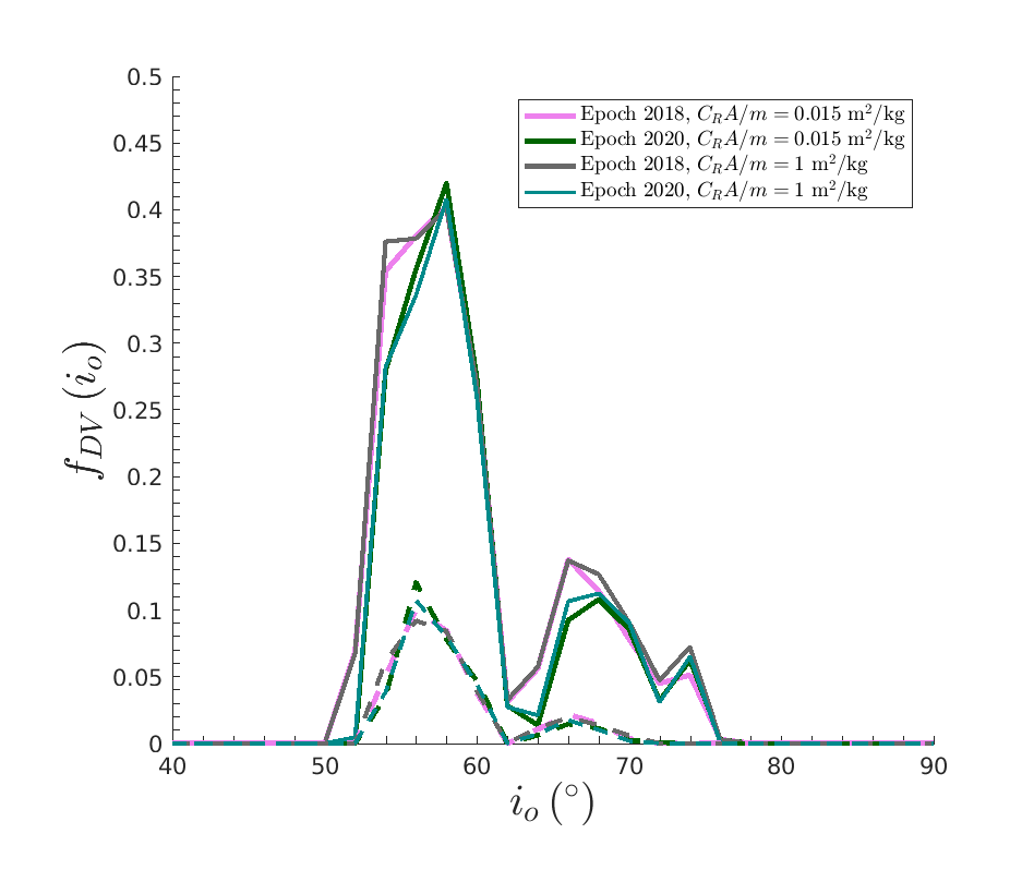
(a) $a_{GLO}$

(b) $a_{GPS}$

(c) $a_{BEI}$

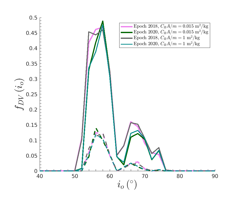
(d) $a_{GAL}$

Figure 13: Frequency of the reentry particles with a limited $\Delta V$, $f_{DV}$, as function of initial inclination (see text for details on their calculation). The color scheme is the same as in Figure 10. The dashed lines refer to an upper limit of $\Delta V=300$ m/s, whereas the solid ones refer to an upper limit of $\Delta V=600$ m/s. For each figure we assumed a starting orbit with fixed $\left(a,e,i\right)$ and various values of $\left(\Omega,\omega\right)$; $\left(a_{GLO},e_{nom},i_{o}\right)$ (top left), $\left(a_{GPS},e_{nom},i_{o}\right)$ (top right), $\left(a_{BEI},e_{nom},i_{o}\right)$ (bottom left), $\left(a_{GAL},e_{nom},i_{o}\right)$ (bottom right).

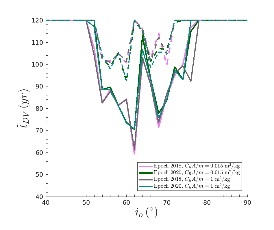
(a) $a_{GLO}$

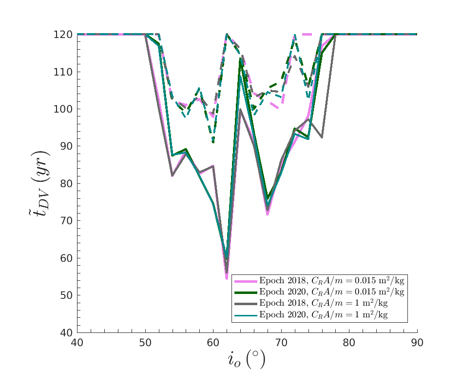
(b) $a_{GPS}$

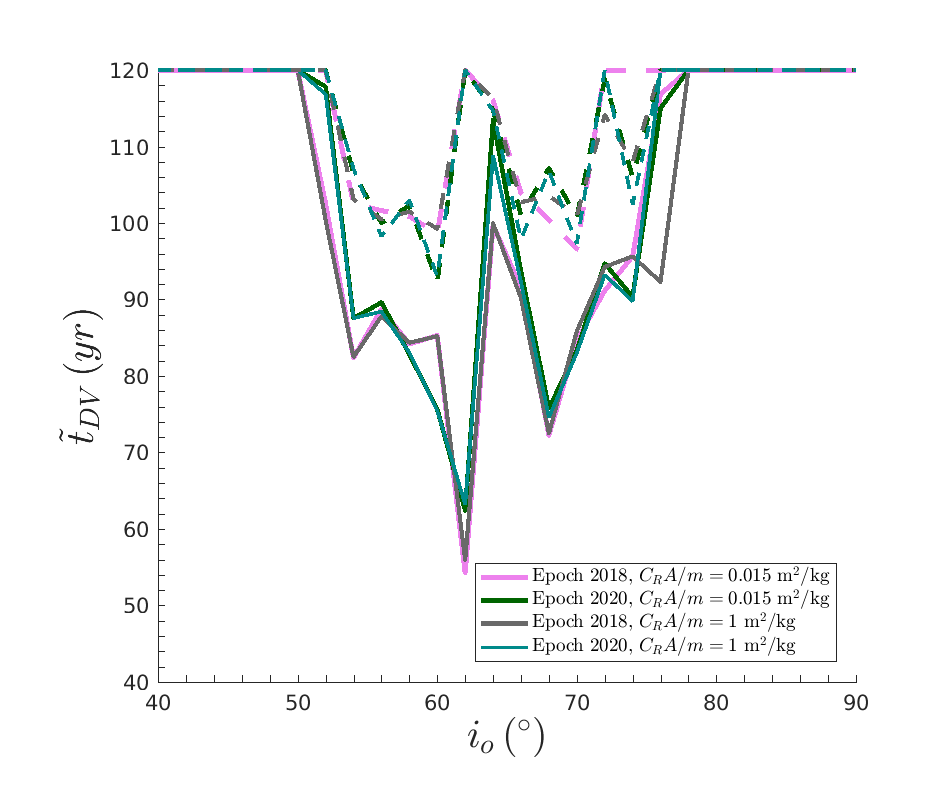
(c) $a_{BEI}$

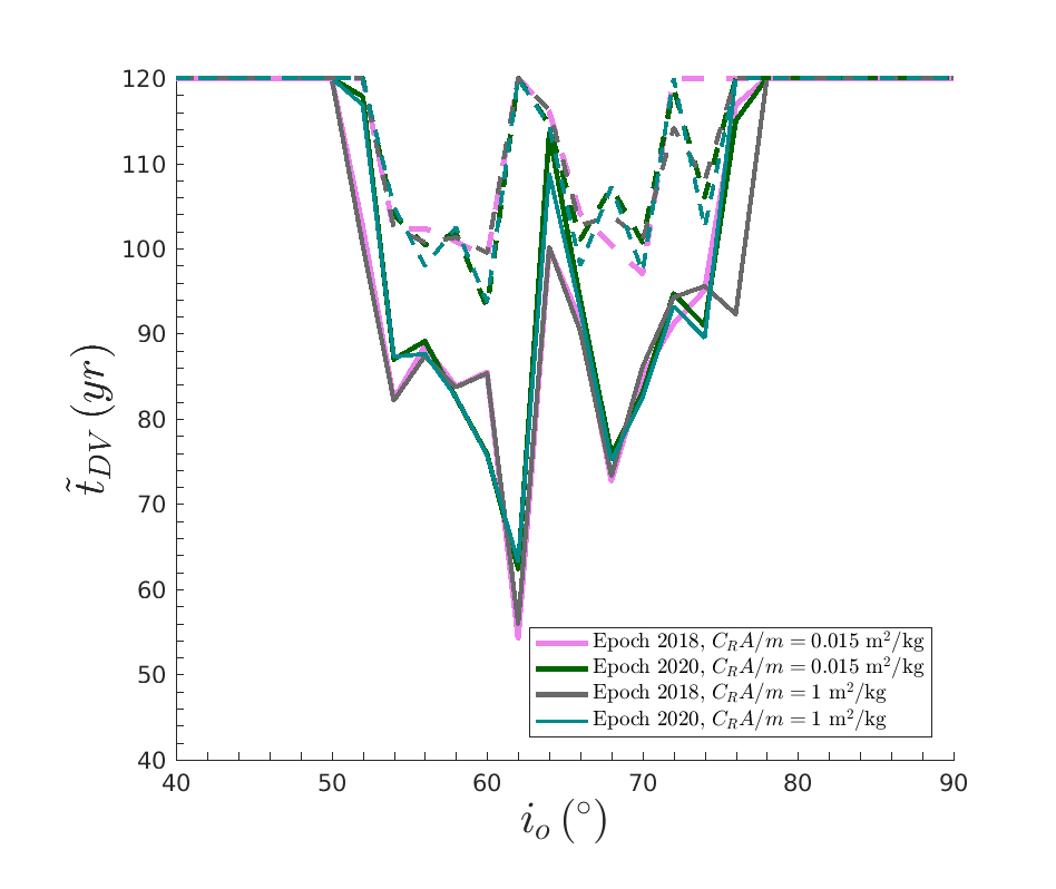
(d) $a_{GAL}$

Figure 14: Mean dynamical lifetime of the reentry particles with a limited $\Delta V$, $\tilde{t}_{DV}$, as function of initial inclination (see text for details on their calculation). The color and line scheme is the same as in Figure 13.

We computed the required $\Delta V$ for these types of maneuvers, starting from orbits with given $\left(a,e,i\right)$ and for all combinations of $\left(\Omega,\omega\right)$. We chose nearly circular initial orbits ($e=10^{-4}$) with $a=a_{GLO},a_{GPS},a_{BEI}$ and $a_{GAL}$ and any inclination $i=i_{o}$ used in our MEO-general grid. For each starting orbit we target all respective reentry solutions, as found in the MEO-general study. Figure 13 shows the frequency of the reentry population that can be reached with maximum $\Delta V=300$ m/s (dashed lines) or $600$ m/s (solid lines), as functions of $i_{o}$. The higher value of maximum $\Delta V$ used here is taken in compliance to Radtke et al. (2015) and Armellin and San-Juan (2018). Figure 14 shows the mean dynamical lifetime of the reentry solutions reached with maximum $\Delta V=300$ m/s or $\Delta V=600$ m/s, as functions of $i_{o}$. The color scheme is the same as in Figure 10. For low to moderate inclinations (up to $\sim 45^{\circ}$) and for really high inclinations ($>\sim 80^{\circ}$), no reentry solution can be reached from an initially quasi-circular orbit, even with $\Delta V\leq 600$ m/s. For inclinations around $56^{\circ}$, $\sim 45-50\%$ of the reentry solutions, with a mean dynamical lifetime varies $\sim 80-90$ yr, can be reached with $\Delta V\leq 600$ m/s. When an upper limit of $\Delta V=300$ m/s is assumed, only $\sim 15\%$ of the reentry populations could be used for disposing an initially quasi-circular satellite, whereas the mean dynamical lifetime increases to $\sim 100$ yr. For inclinations near $\sim 64^{\circ}$, $\sim 15\%$ and $\sim 3\%$ of the reentry solutions can be reached with $\Delta V\leq 600$ m/s and $\Delta V\leq 300$ m/s, respectively, the corresponding mean dynamical lifetime being $\sim 75$ yr and $\sim 100$ yr. Note that, as in the general MEO case, the results do not vary a lot with the choice of initial epoch and $C_{R}A/m$.

Focusing at the GNSS constellations, we performed the same study starting from typical GNSS orbits with $e_{0}=10^{-4}$, and varying orientations. We targeted final orbits among our reentry solutions database, and graveyard solutions found in our GNSS- graveyard study. Given our MEO grid’s resolution, when looking for reentry solutions we set the inclination of the starting orbit to $i_{o}=56^{\circ}$ (for GPS, BEIDOU and GALILEO) or $i_{o}=64^{\circ}$ (GLONASS).When looking for graveyard solutions, we set $i_{o}=i_{nom}$ for each group. Figure  15 shows the $\Delta V$ required vs the lifetime of the reentry orbit and Figure 16 shows the $\Delta V$ required vs $e_{max}$ of the graveyard orbit. For the reentry solutions, one can see two ‘V-shaped’ clouds of points in every graph; these correspond to single- and two-burn (bi-elliptic) transfers. The lower envelopes (red and blue curves) of these V-shaped clouds approximately constist of the respective ‘optimal’ solutions with respect to lifetime, i.e., approximately constitute what are known as atmospheric reentry Pareto fronts (Armellin and San-Juan, 2018). Reentry solutions with small lifetimes (of decadal order) cannot be reached due to very high cost ($\Delta V\geq 300$ m/sec). Note also that the cost of a single-burn transfer is twice of that for a two-burn transfer for lifetimes smaller than $\sim 80$ yr (for GPS, BEIDOU and GALILEO) or $\sim 110$ yr (for GLONASS). There exist reentry solutions with $\Delta V<300$ m/sec and lifetime $\sim 80$ yr, but they are not equally numerous at every $\left(\Omega,\omega\right)$ configuration.

For the graveyard solutions (Fig. 16), one can see ‘triangle-shaped’ clouds of points; those all correspond to two-burn transfers, as graveyard orbits cannot cross the operational GNSS regions by definition. The lower envelop (blue curve) consists of the respective optimal solutions, where $\Delta V$ is roughly proportional to $e_{max}$. In general, the $\Delta V$ needed to transfer to a graveyard orbit is quite small, $\sim 5-40$ m/sec, as opposed to a reentry orbit. Note that similar results were found by Mistry and Armellin (2016) for the GALILEO case. Moreover, the lower $e_{max}$, the more likely for a graveyard orbit to remain ‘stable’ for times longer than $200$ yr. Of course, it is not clear how many disposed satellites one could safely store in these narrow graveyards bands, and such computations likely require a more accurate dynamical model.

One of the goals of the ReDSHIFT is the development of a software toolkit that would enable an informed design of “debris compliant” missions, including the design of an appropriate passive removal strategy, given an operational orbit and $\Delta V$ budget. We refer the reader to Rossi et al. (2018) for a in-depth discussion about the software toolkit. The results presented in this paper have been collected in the form of a database of pre-computed solutions, to be used as input in the software toolkit. Of course, the database is expandable and we hope to keep expanding it in the future. An example of the typical output that this toolkit should give for a MEO mission is shown in Figures 15,16,17.

In Table 4, the initial conditions for a set of starting orbits are given. Corresponding to these starting orbits, the ‘optimal’ solutions are shown in Table 5 where, along with ($a,e$) values, the $\Delta V$ spent on the transfer and the waiting time $T$ of reentry are shown. Two reentry solutions are given for each starting orbit, labeled as $\Delta V$-optimal and $T$-optimal, corresponding to a minimum $\Delta V$ or a minimum $T$. Similarly, in Table 6 the $\Delta V$-optimal graveyard solution for each starting orbit is given. In Figure 17 the time evolution of $a$, $e$ and $i$ of the $\Delta V$-optimal reentry (left), $T$-optimal reentry (middle) and $\Delta V$-optimal graveyard (right) solutions for each GNSS representative, is shown. Note that, for the purposes of the software toolkit, we have run again all our reentry solutions, adding atmospheric drag, with a simple density model described in Skoulidou et al. (2018). We verified that our chosen limit of $q=R_{E}+400$km in the drag-free case was adequate for identifying reentry solutions, while the differences found in reentry time between the former and the latter propagation are minute. One can clearly see the footprint of atmospheric drag at the final instances of the orbits shown in Fig 17, where both $a$ and $e$ drop abruptly.

The initial eccentricity of the ‘optimal’ reentry solutions varies between $0.08-0.16$ and the lifetime for most of them is near $110$ yr. The $\Delta V$ budget required for these transfers varies in the range $150-300$ m/sec. Again, the results depend strongly on the choice of $\left(\Omega,\omega\right)$ for the starting orbit. Hence, it is possible to find ‘optimal’ solutions with $\sim 70$ yr lifetime and $\Delta V\sim 300$ m/sec, as also shown in Figure 15. On the other hand, all $\Delta V$-optimal graveyard solutions start as circular orbits, and their eccentricities reach up to $\sim 0.01$ within 200 years. Note that some of these evolutions suggest that eccentricities may in fact increase further and hence violate the boundaries of the operational zones, at times much longer than 200 years, however. The $\Delta V$-budget for transfer to these graveyards is $\leq 23$ m/sec. Note that the ‘optimal’ solutions found here are among the set of evaluated solutions presented in Section 3, but the real optimal transfer may correspond to a more favorable choice of $\omega$.

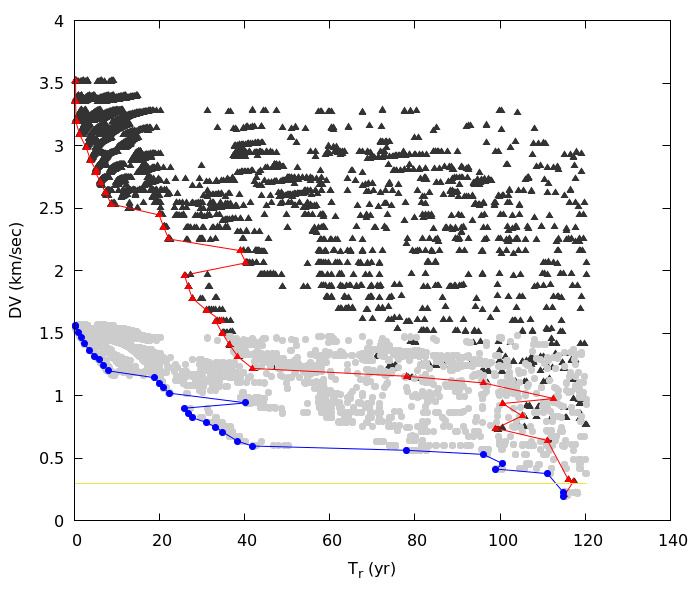
(a) GLONASS

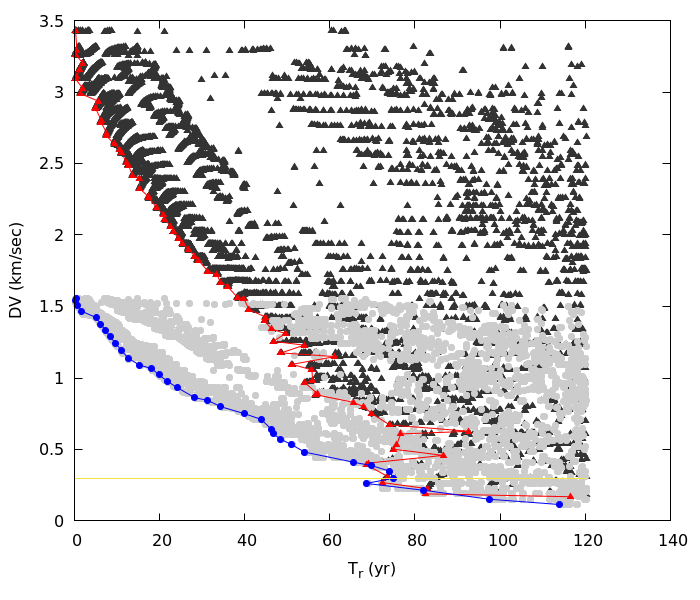
(b) GPS

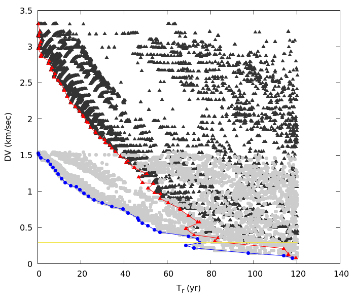
(c) BEIDOU

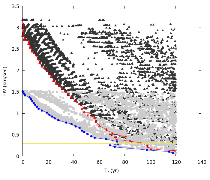
(d) GALILEO

Figure 15: $\Delta V$-lifetime maps for reentry solutions found around typical GLONASS (top left), GPS (top right), BEIDOU (bottom left) and GALILEO (bottom right) orbits. Light gray points correspond to solutions using a two-burn method (bi-elliptic transfers). Dark gray points correspond to solutions using a single-burn method. Blue and red lines are the Pareto fronts of the two-burn and single-burn method, respectively. Yellow line corresponds to $\Delta V=300$ m/sec.

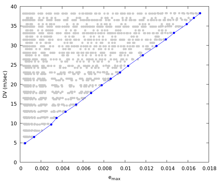
(a) GLONASS

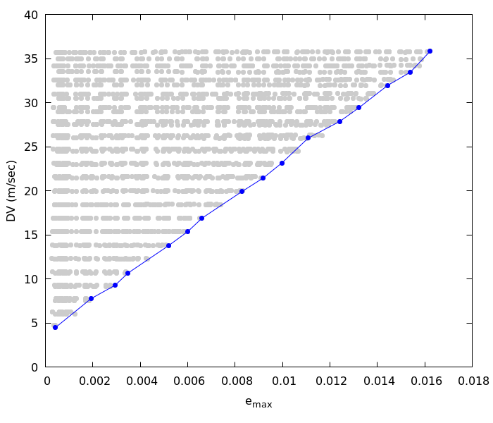
(b) GPS

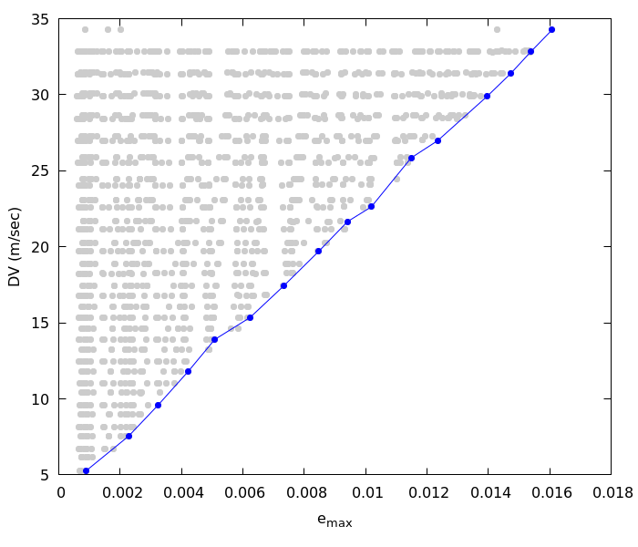
(c) BEIDOU

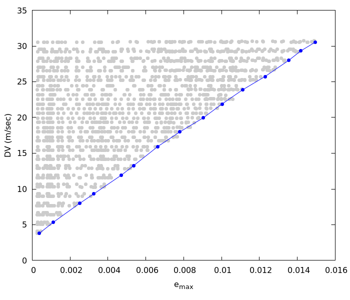
(d) GALILEO

Figure 16: $\Delta V-e_{max}$ maps for graveyard solutions found around typical GLONASS (top left), GPS (top right), BEIDOU (bottom left) and GALILEO (bottom right) orbits using a two-burn method (bi-elliptic transfer for nearly zero $e$, i.e., Hohmann-like). Blue lines are the Pareto fronts of the two-burn method.

Table 4: Initial choice of $a$, $e$, $i$, $\Omega$ and $\omega$ of assumed operational orbits.

	$a$	$e$	$i$ (deg)	$\Omega$ (deg)	$\omega$ (deg)
GLONASS	$a_{GLO}$	$0.0001$	$64.00/64.80$	$102.83$	$106.50$
GPS	$a_{GPS}$	$0.0001$	$56.00/55.00$	$~{}12.83$	$106.50$
BEIDOU	$a_{BEI}$	$0.0001$	$56.00/55.00$	$102.83$	$106.50$
GALILEO	$a_{GAL}$	$0.0001$	$56.00$	$192.83$	$106.50$

Table 5: $\Delta V$-optimal and $T$-optimal reentry orbits for the assumed operational orbit

	optimal	$a\left(km\right)$	$e$	$\Delta V$ (m/sec)	$T\left(yr\right)$
GLONASS	$\Delta V$	$28249.99$	$0.1000$	$192.8$	$115.22$
	$~{}T$	$28355.40$	$0.1000$	$193.7$	$114.85$
GPS	$\Delta V$	$26985.07$	$0.1200$	$228.6$	$117.52$
	$~{}T$	$26985.07$	$0.1200$	$228.6$	$117.52$
BEIDOU	$\Delta V$	$28882.46$	$0.0800$	$148.6$	$116.16$
	$~{}T$	$29514.92$	$0.1600$	$294.1$	$~{}80.71$
GALILEO	$\Delta V$	$29936.56$	$0.1000$	$180.9$	$115.19$
	$~{}T$	$29304.10$	$0.1600$	$290.3$	$~{}99.21$

Table 6: $\Delta V$-optimal graveyard orbits for the assumed operational orbit

	optimal	$a\left(km\right)$	$e$	$\Delta V$ (m/sec)	$e_{max}$
GLONASS	$\Delta V$	$25593.65$	$0.0000$	$6.5$	$0.00081$
GPS	$\Delta V$	$26479.10$	$0.0000$	$6.0$	$0.00070$
BEIDOU	$\Delta V$	$28018.09$	$0.0000$	$7.6$	$0.00228$
GALILEO	$\Delta V$	$29240.85$	$0.0000$	$22.5$	$0.00997$

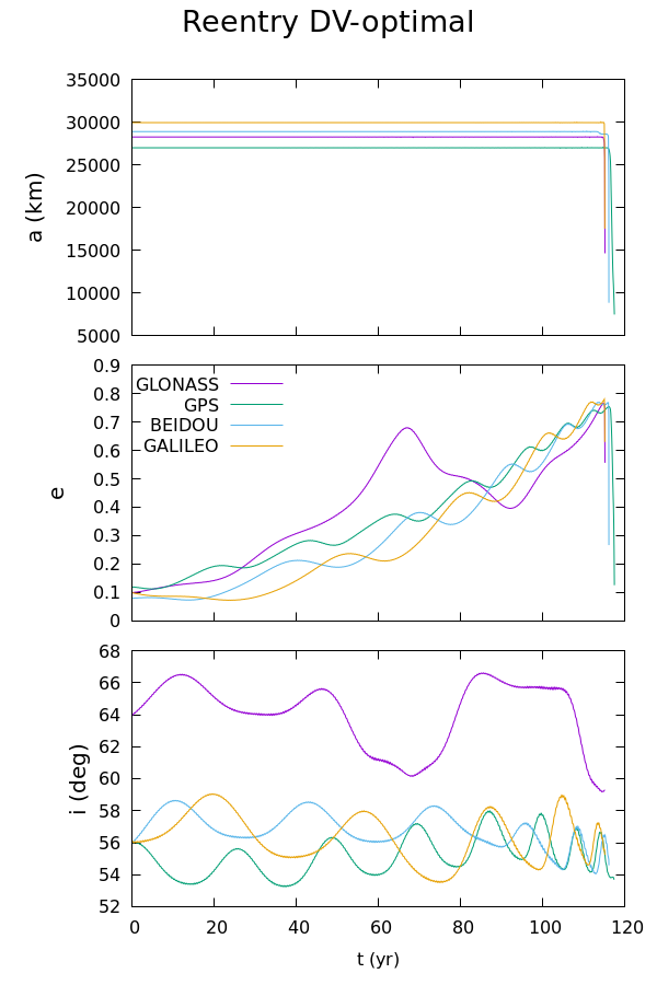
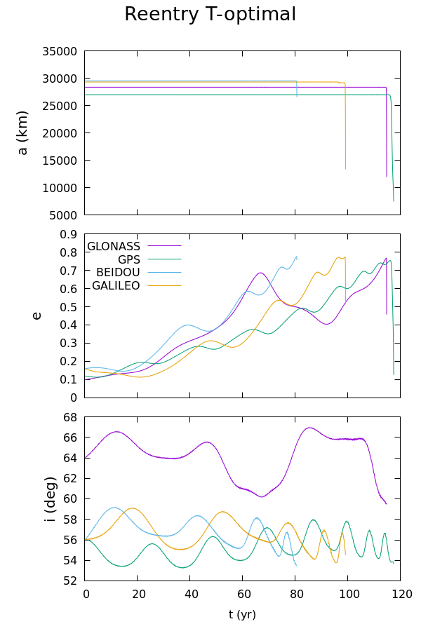
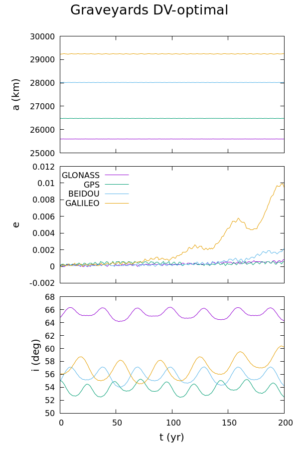
Figure 17: Evolution of $a$, $e$, and $i$ of $\Delta V$-optimal (left) and $T$-optimal (middle) reentry solutions and of $\Delta V$-optimal (right) graveyard solutions, for four typical starting orbits, one for each GNSS group.

5 Conclusions

We presented our results from a study on the long-term dynamics in the extended MEO/GNSS orbital region, using a dynamical model that consisted of the second degree and order geopotential, lunisolar perturbations, and SRP (cannonball model). In total, about 6 million orbits were propagated for a time equivalent to $120-200$ yr, for two different initial epochs, and two values of the $C_{R}A/m$ ratio. The aim of this study was to construct a detailed dynamical atlas and use it to locate suitable reentry and graveyard solutions, which could be useful for designing EoL strategies.

As shown by our results, the most interesting and complex dynamical behavior appears for moderate-to-high inclinations ($\sim 40^{\circ}-70^{\circ}$), where the GNSS groups are actually placed. In particular, the number of reentry solutions seems to maximize around three particular inclination ‘zones’ (around $i=$46, 56, and 68 degrees); this result seems to be roughly independent of $A/m$ as well as of the initial epoch, chosen here. However, as noted already, more initial epochs (and more distant ones), leading to diverse values of the lunar ascending node should be studied, before concluding that this structure is epoch-invariant. For the same inclination bands, the mean dynamical lifetime of reentry orbits minimizes. It is already known from previous studies that secular lunisolar resonances are actually dominating the dynamics at those inclinations. The variations of a satellite’s eccentricity and inclination may lead to perigee decrease and eventually, atmospheric reentry. In the region around $56^{\circ}$, reentry dynamical hatches appear even for low-to-moderate eccentricities (e.g., reentry orbits with initial $e\sim 0.10$ and lifetimes of $\sim 60$ yr), with a strong dependence on secular angle configuration. On the other hand, around $64^{\circ}$ the reentry dynamical hatches appear generally for higher eccentricities. An enhanced $C_{R}A/m$ value extends the reentry regions and decreases the time required for reentry by a decade or so, but does not significantly alter the overall structure of the $\left(a,e\right)$ map. The reachability of all reentry solutions from a nearly-circular initial orbit, using single- and two-burn maneuvers, was studied (coaxial and coplanar elliptical orbits). For GNSS altitudes we find that the $\Delta V$ budget needed is roughly inversely proportional to the orbital lifetime (waiting time). Typically, reentry solutions with $\Delta V<300$ m/s have lifetimes longer than $\sim 70$yr. Note that this study did not focus on the computation of globaly optimal reentry solutions; this would require adopting a different strategy of optimizing $\Delta V$ (e.g. as in Armellin and San-Juan (2018)), or studying a much finner grid in ($\omega,\Omega$). Instead, we decided to focus on exporing the whole domain of inclinations, which had not been extensively studied so far, at the same time as studying the feasibility of using the dynamical maps for finding near-optimal reentry solutions. Clearly, our results need to be extended, especially in the current operational GNSS region.

A dedicated study for the graveyard regions around the four GNSS groups revealed that the percentage of bodies initially placed in graveyard regions and surviving for time spans of $200$ yr is $\sim 20-40$%. These regions are limited to a maximum eccentricity of $\sim 0.018$, but such mildly eccentric graveyard solutions exist. The results vary of course with secular angles orientation. However, as our definition of the graveyard regions is quite generous, the surviving solutions seem abundant and easily targeted by two-burn maneuvers with $\Delta V\in 5-40$ m/sec. Note that $\Delta V$ is roughly proportional to the maximum eccentricity attained during the $200$ yr orbital evolution.

One of the goals of the ReDSHIFT project is to provide a toolkit for designing “debris-friendly” passive EoL strategies for future satellites missions. Hence, the study presented here provides a database of solutions to be used in that toolkit. We intend to further expand this database, by propagating a more extensive grid of initial conditions, for various epochs and $\omega$-orientations. This will also allow a deeper understanding of the long-term extended MEO dynamics. We expect to be able to present our results in the near future.

Appendix A Dynamical maps of MEO-general grid

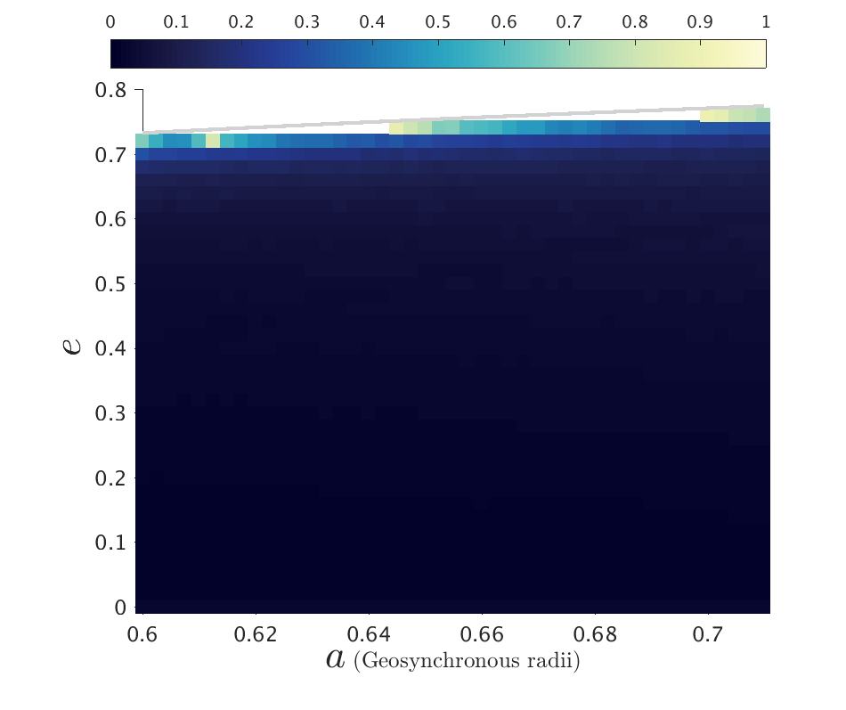
(a) $\bm{i}_{o}={\bf 0}$

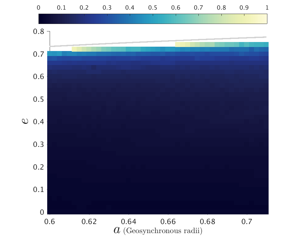
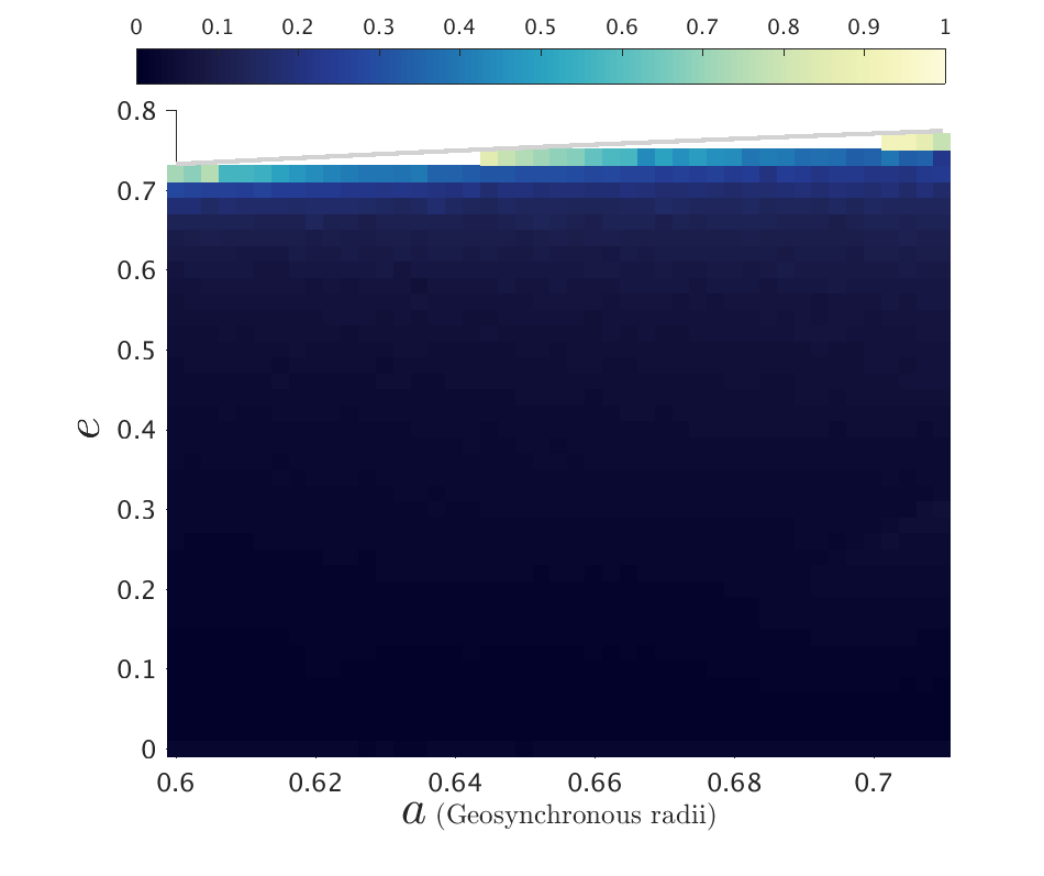
(b) $\bm{i}_{o}={\bf 28^{\circ}}$

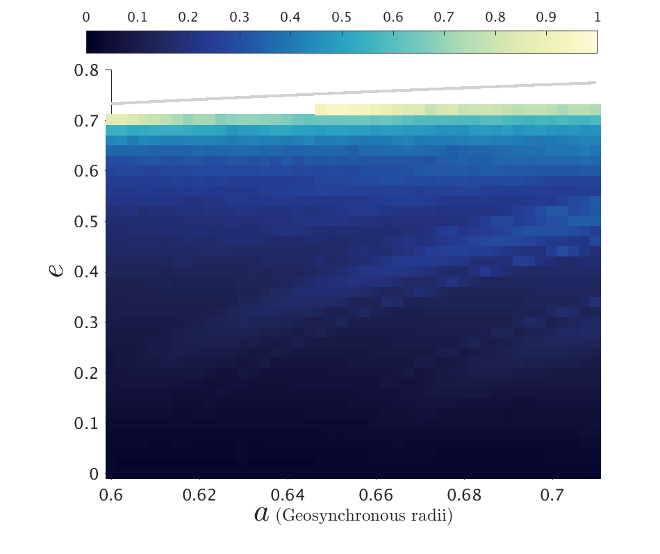
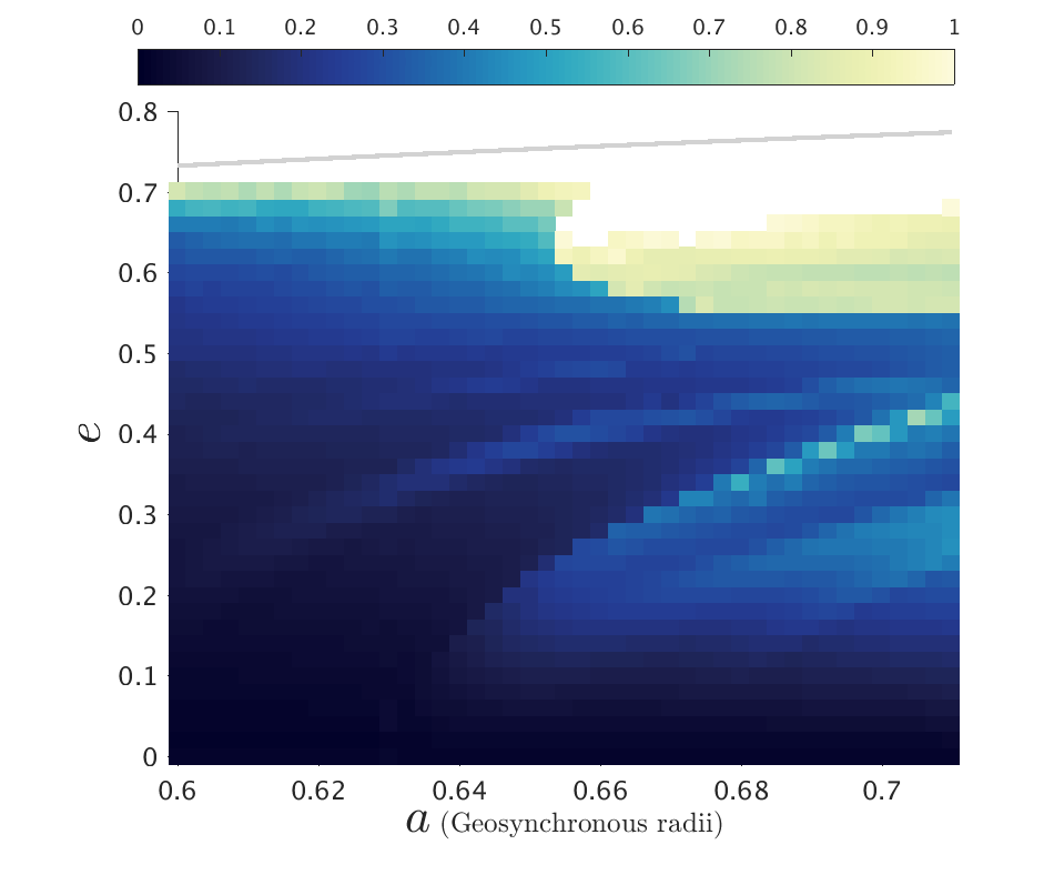
(c) $\bm{i}_{o}={\bf 44^{\circ}}$

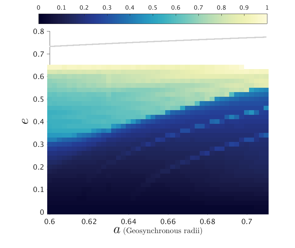
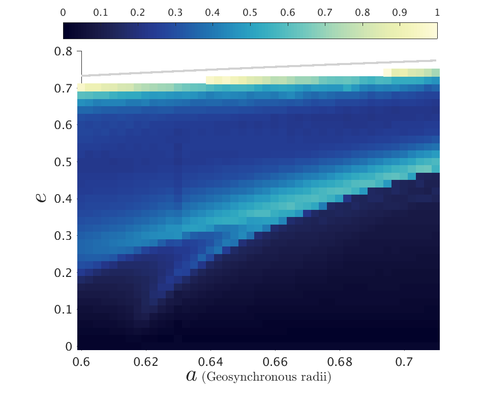
(d) $\bm{i}_{o}={\bf 46^{\circ}}$

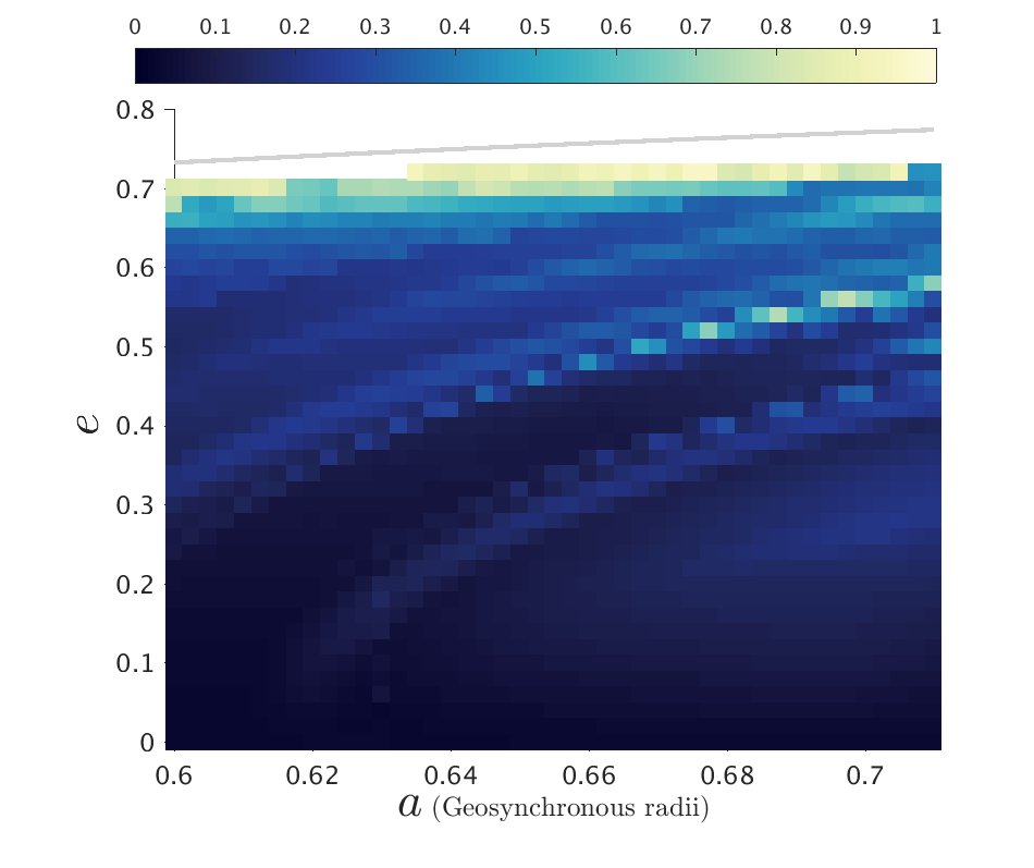
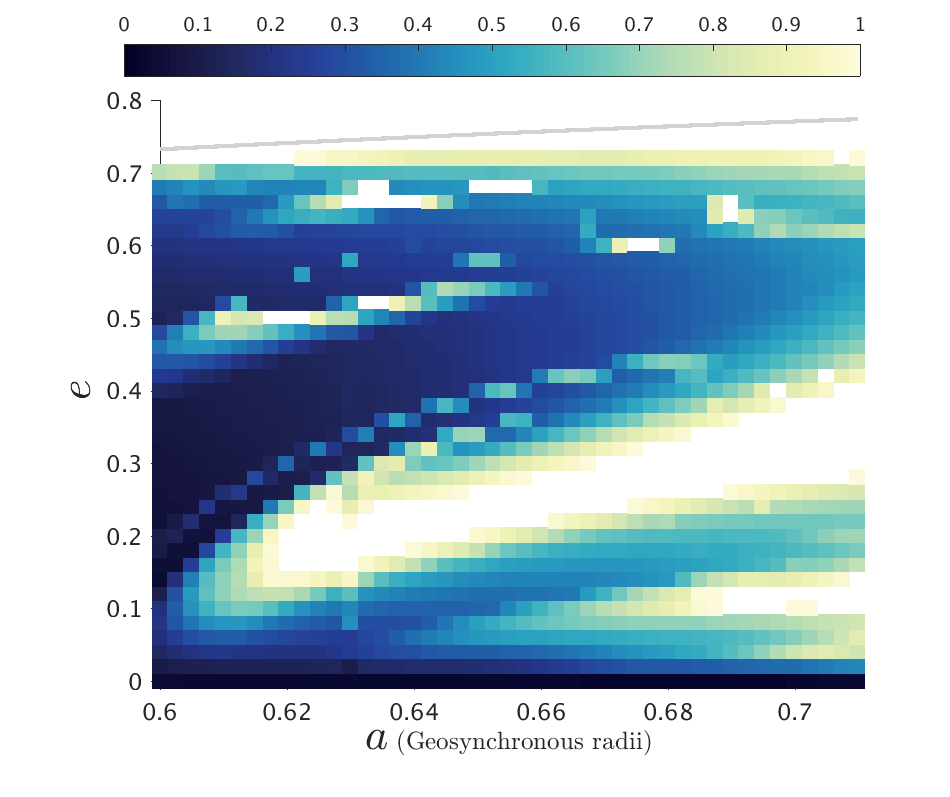
(e) $\bm{i}_{o}={\bf 54^{\circ}}$

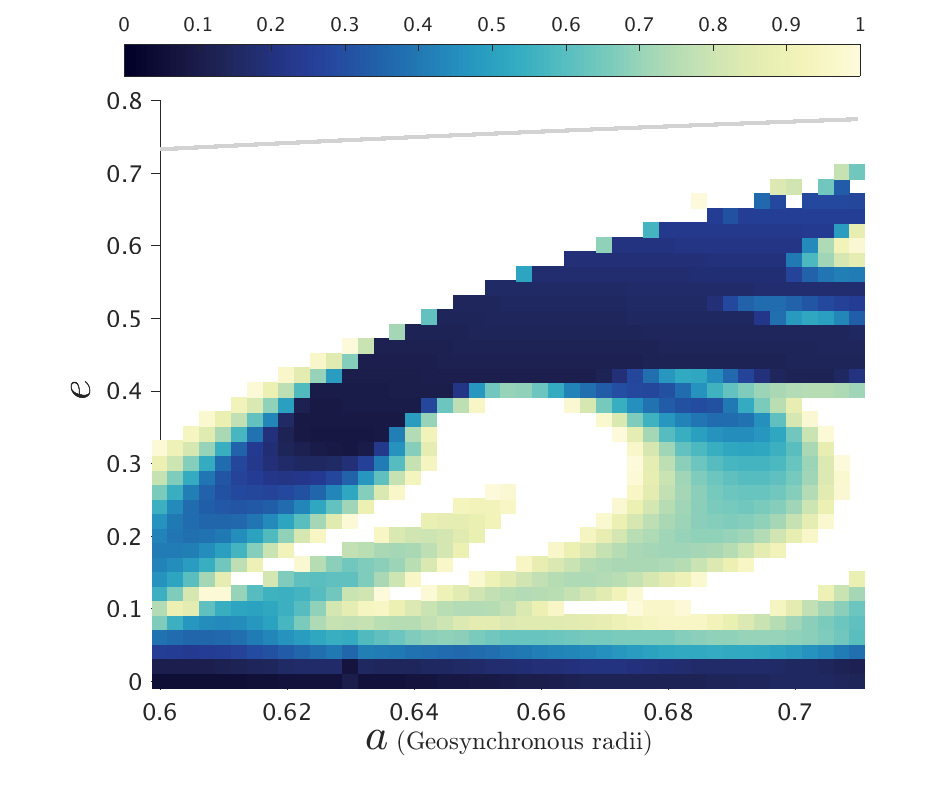
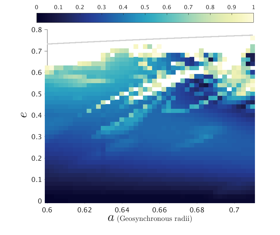
(f) $\bm{i}_{o}={\bf 58^{\circ}}$

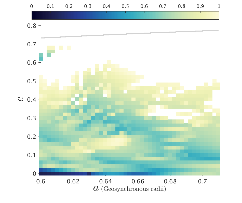
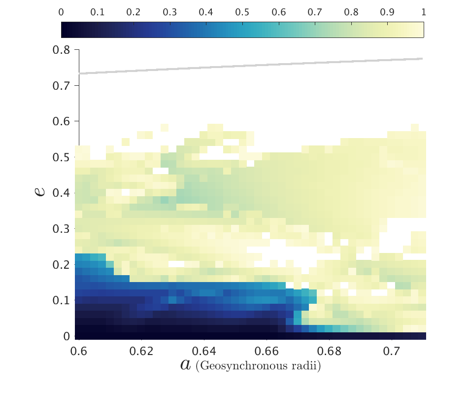
(g) $\bm{i}_{o}={\bf 66^{\circ}}$

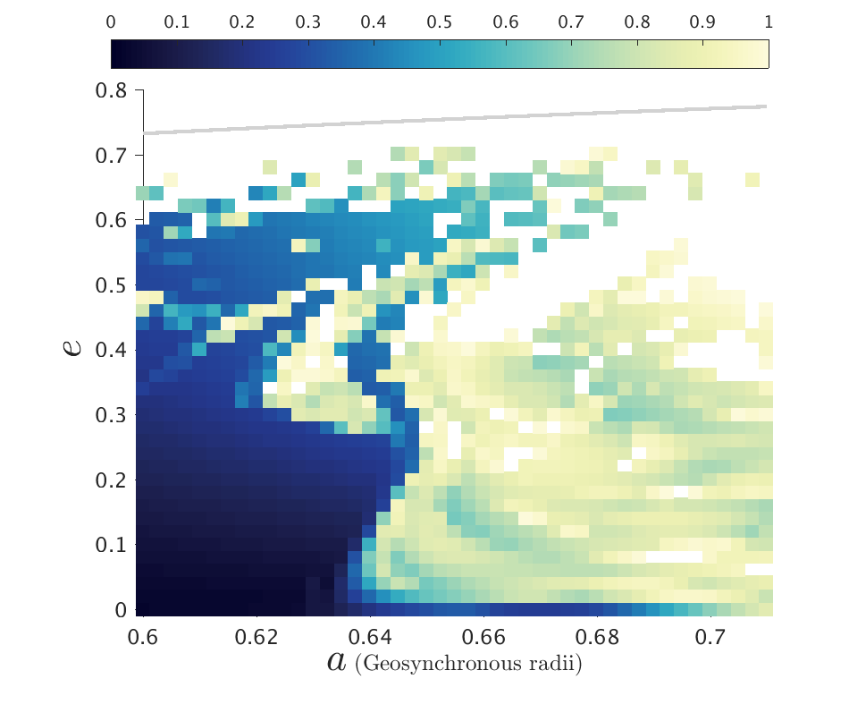
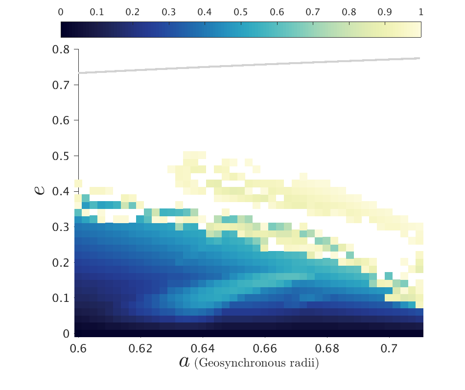
(h) $\bm{i}_{o}={\bf 68^{\circ}}$

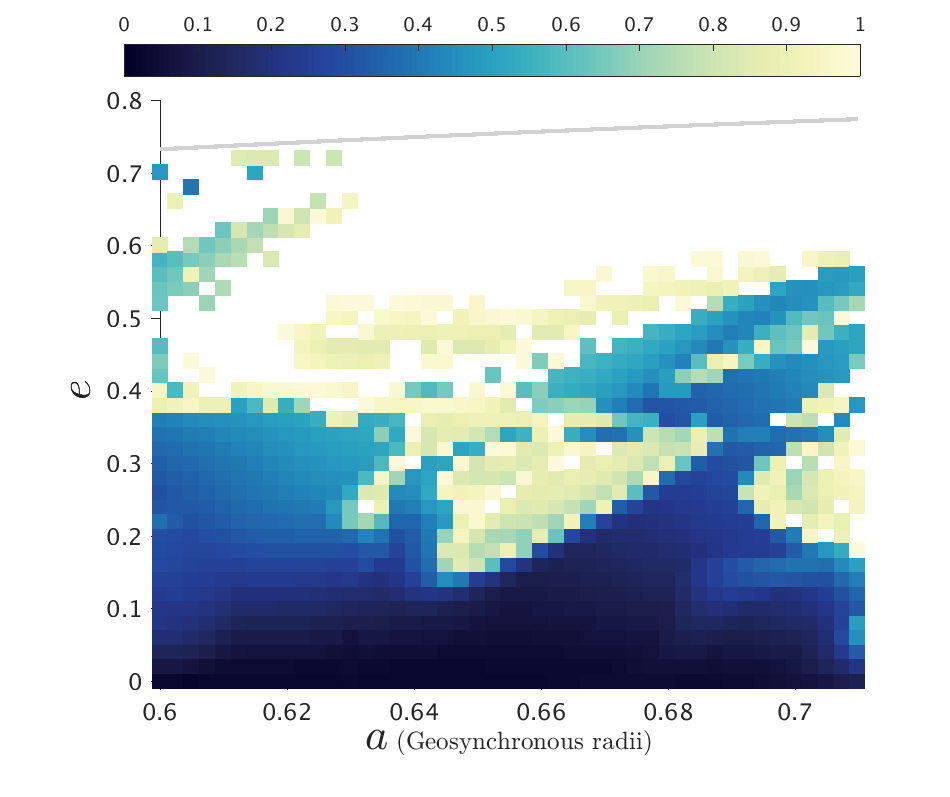
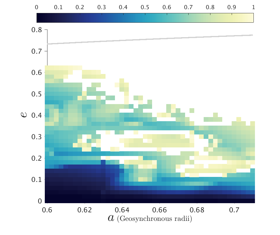
(i) $\bm{i}_{o}={\bf 70^{\circ}}$

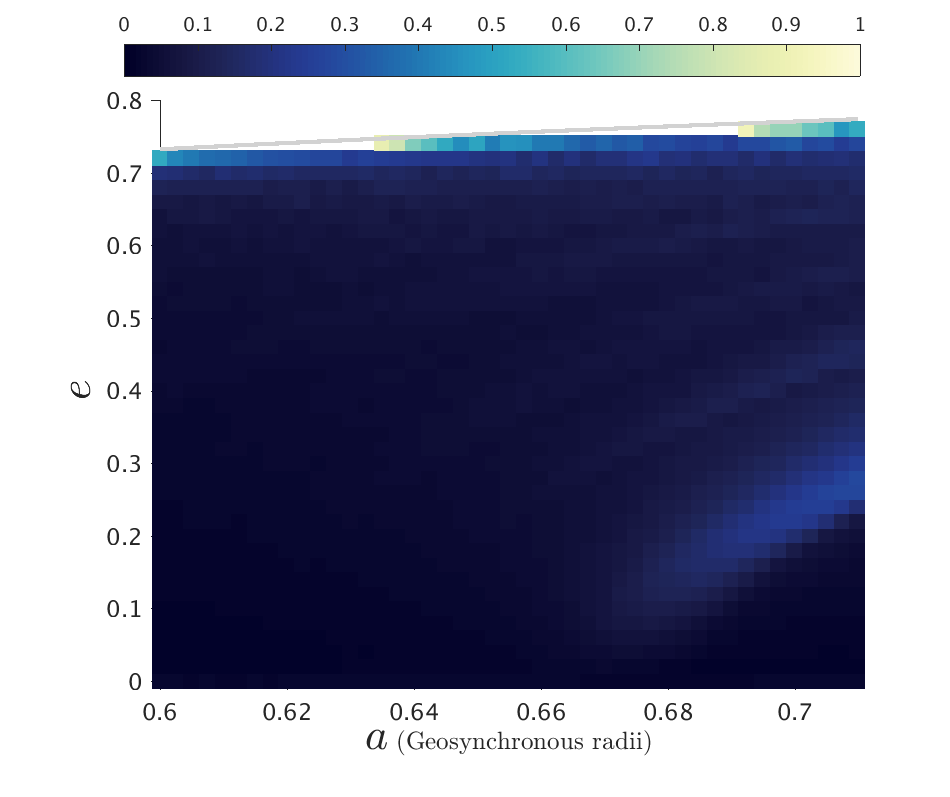
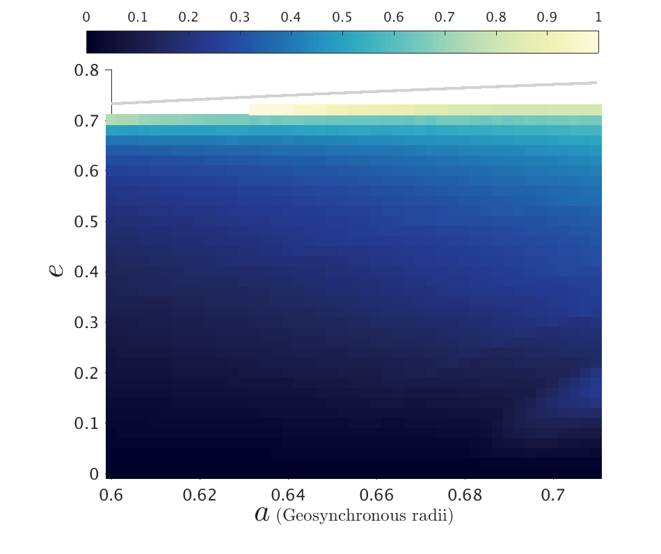
(j) $\bm{i}_{o}={\bf 90^{\circ}}$

Figure 18: $De$ maps of the MEO-general phase space for various $\bm{i}_{o}$, $\bm{\Delta}\bm{\Omega}={\bf 0}$, $\bm{\Delta}\bm{\omega}={\bf 270^{\circ}}$ (1st and 3rd columns) and $\bm{\Delta}\bm{\Omega}={\bf 90^{\circ}}$, $\bm{\Delta}\bm{\omega}={\bf 0}$ (2nd and 4th columns), for Epoch 2018, and for $C_{R}A/m=1$ m²/kg. The colorbar for the $De$ maps is from 0 to 1, where the reentry particles were excluded (white).

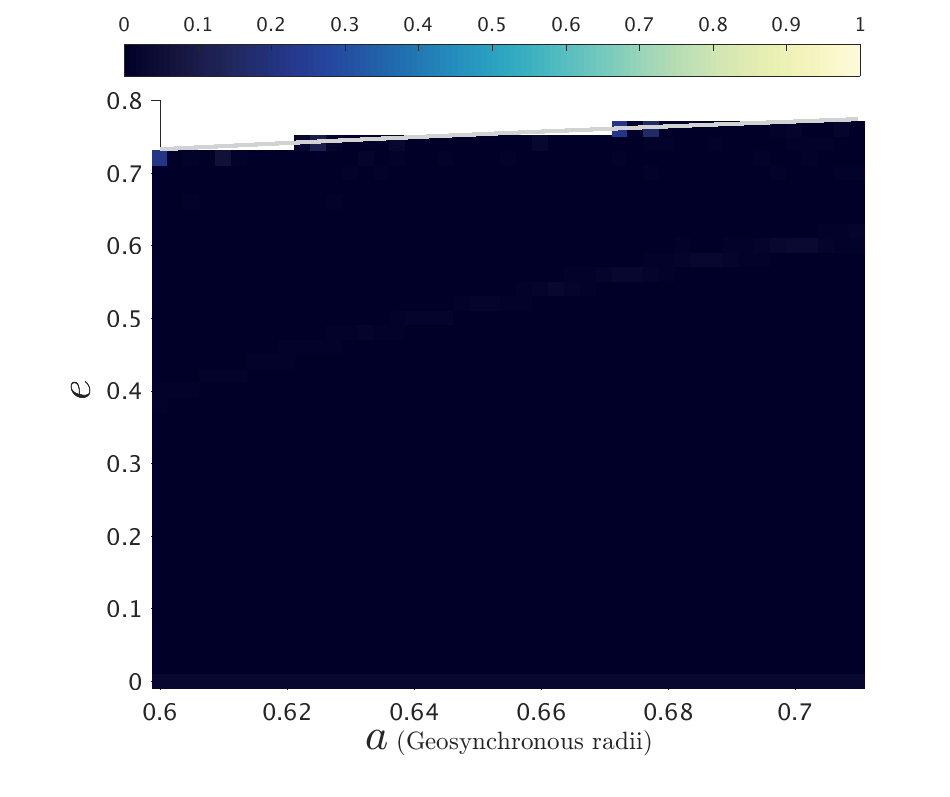
(a) $\bm{i}_{o}={\bf 0}$

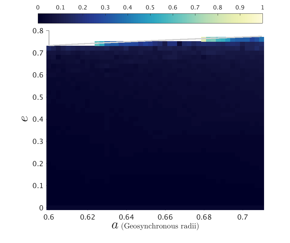
(b) $\bm{i}_{o}={\bf 28^{\circ}}$

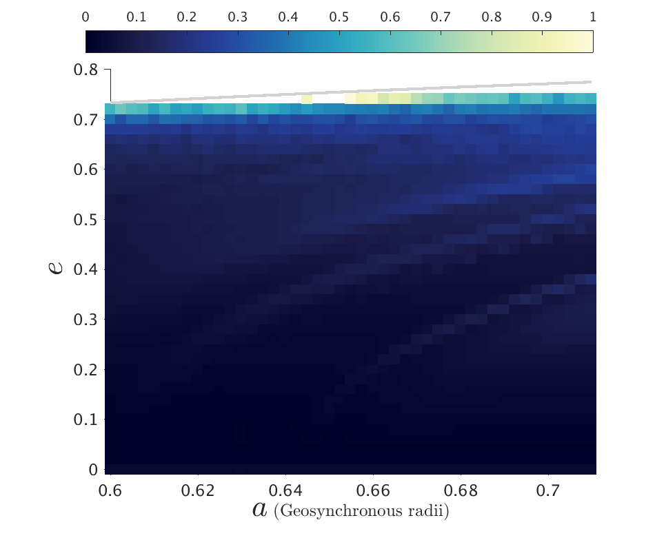
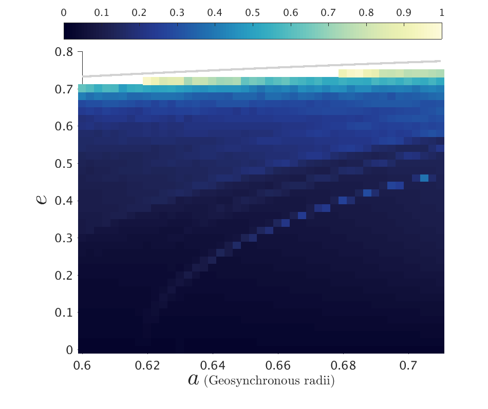
(c) $\bm{i}_{o}={\bf 44^{\circ}}$

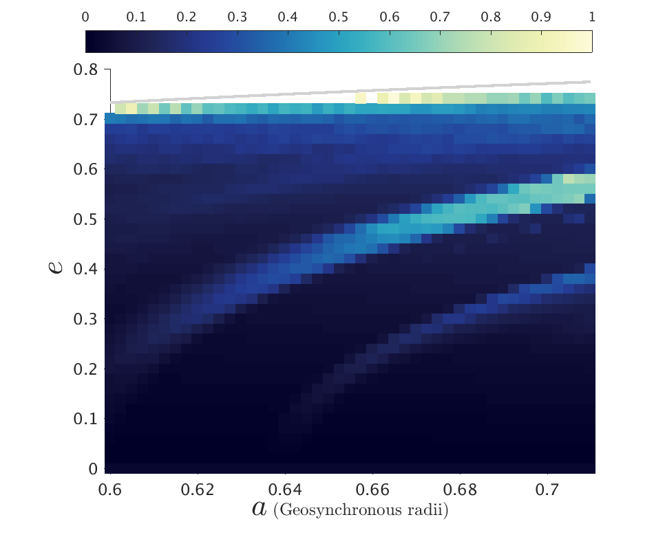
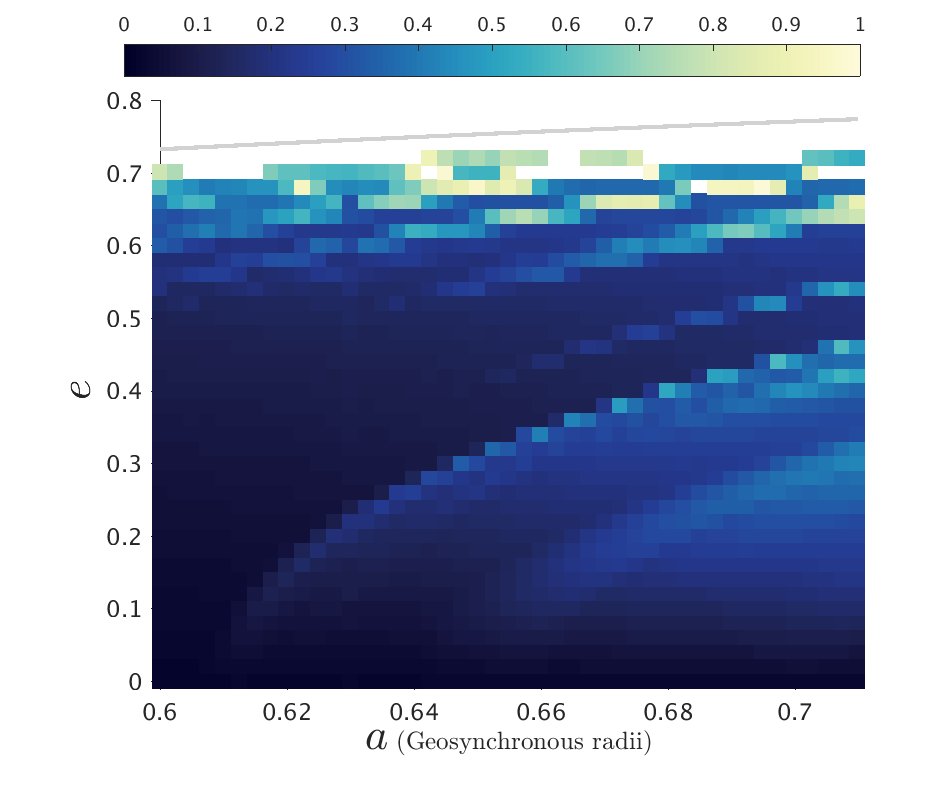
(d) $\bm{i}_{o}={\bf 46^{\circ}}$

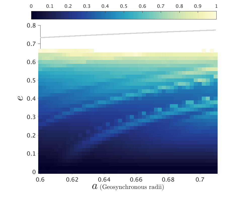
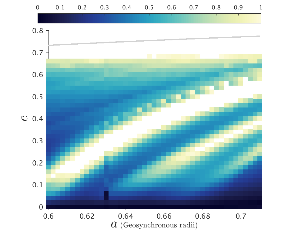
(e) $\bm{i}_{o}={\bf 54^{\circ}}$

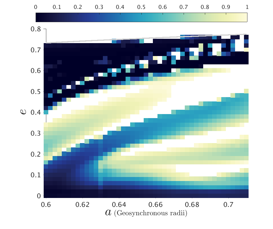
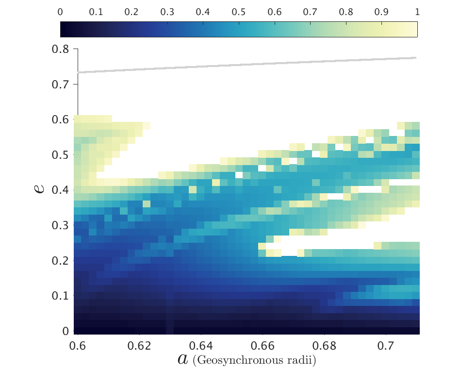
(f) $\bm{i}_{o}={\bf 58^{\circ}}$

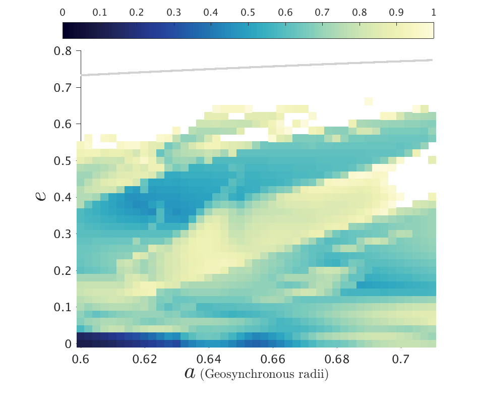
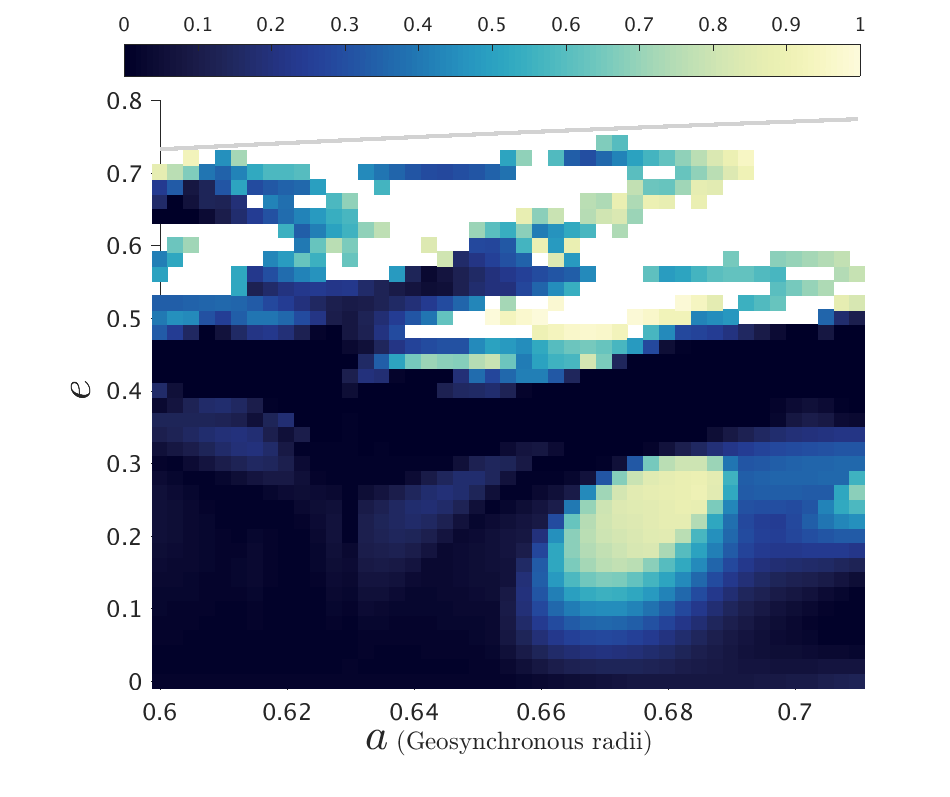
(g) $\bm{i}_{o}={\bf 66^{\circ}}$

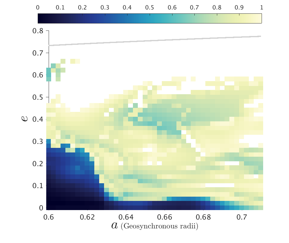
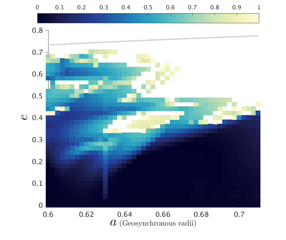
(h) $\bm{i}_{o}={\bf 68^{\circ}}$

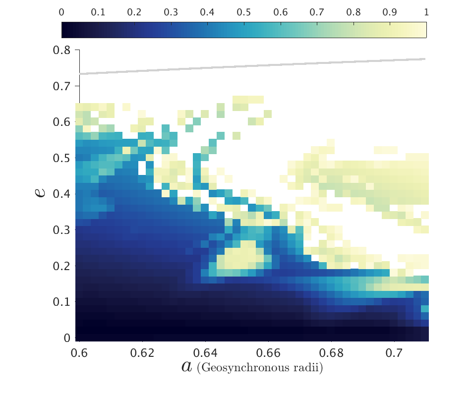
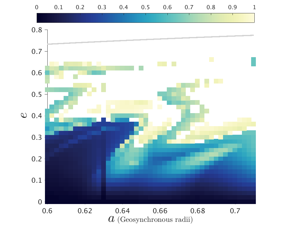
(i) $\bm{i}_{o}={\bf 70^{\circ}}$

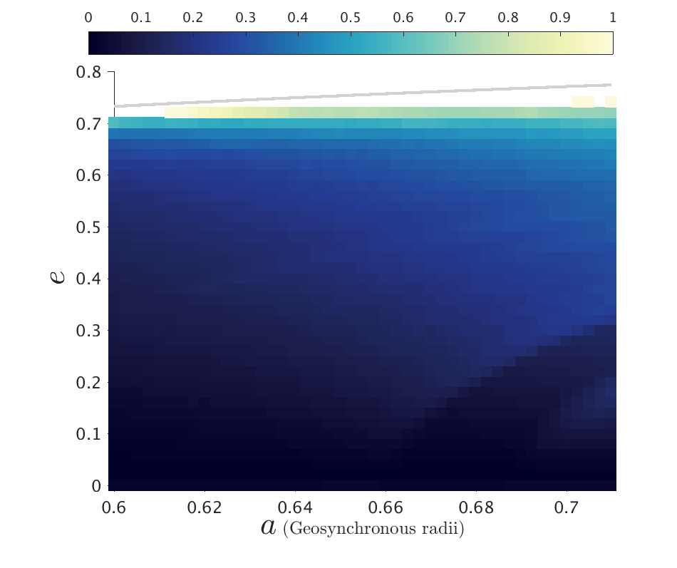
(j) $\bm{i}_{o}={\bf 90^{\circ}}$

Figure 19: $De$ maps of the MEO-general phase space for various $\bm{i}_{o}$, $\bm{\Delta}\bm{\Omega}={\bf 0^{\circ}}$, $\bm{\Delta}\bm{\omega}={\bf 270^{\circ}}$ (1st and 3rd columns) and $\bm{\Delta}\bm{\Omega}={\bf 90^{\circ}}$, $\bm{\Delta}\bm{\omega}={\bf 0}$ (2nd and 4th columns), for Epoch 2020, and for $C_{R}A/m=1$ m²/kg. The colorbar for the $De$ maps is from 0 to 1, where the reentry particles were excluded (white).

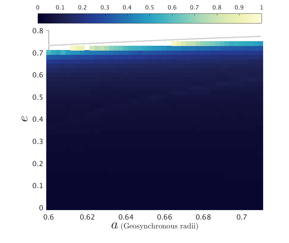
(a) $\bm{i}_{o}={\bf 0}$

(b) $\bm{i}_{o}={\bf 28^{\circ}}$

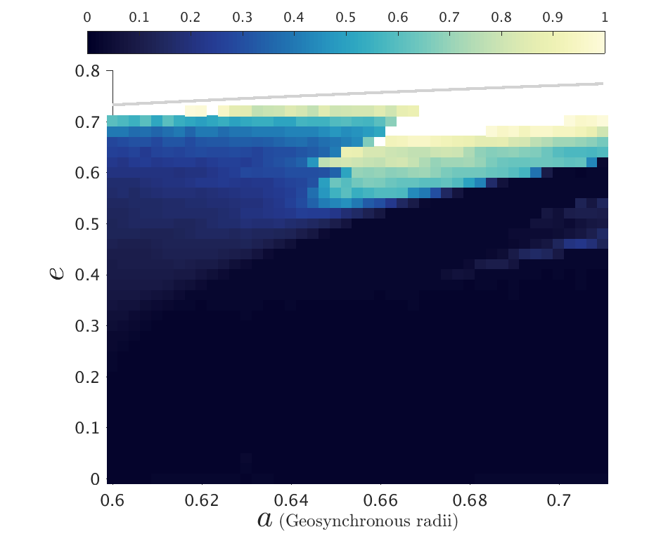
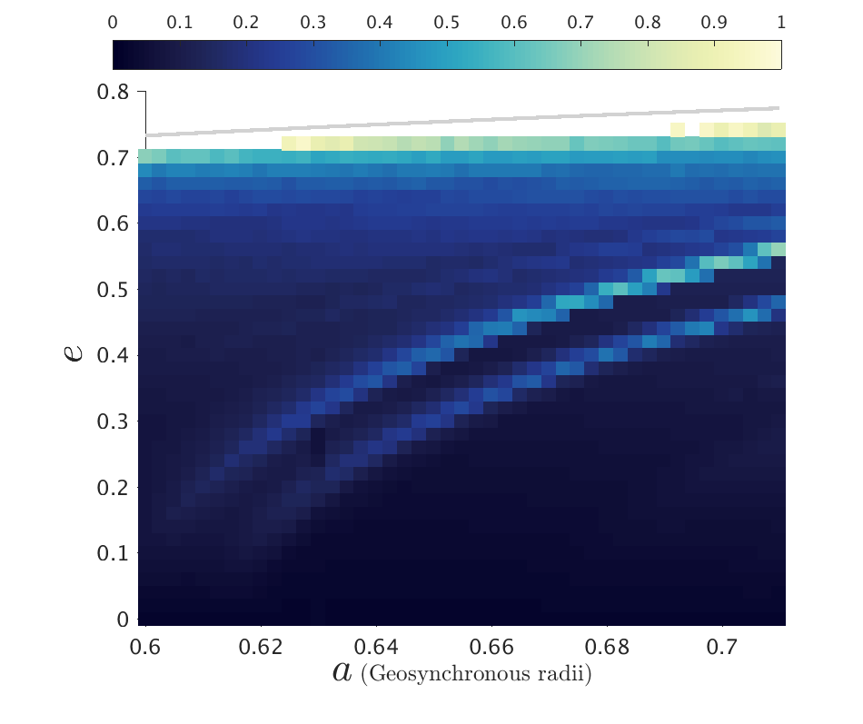
(c) $\bm{i}_{o}={\bf 44^{\circ}}$

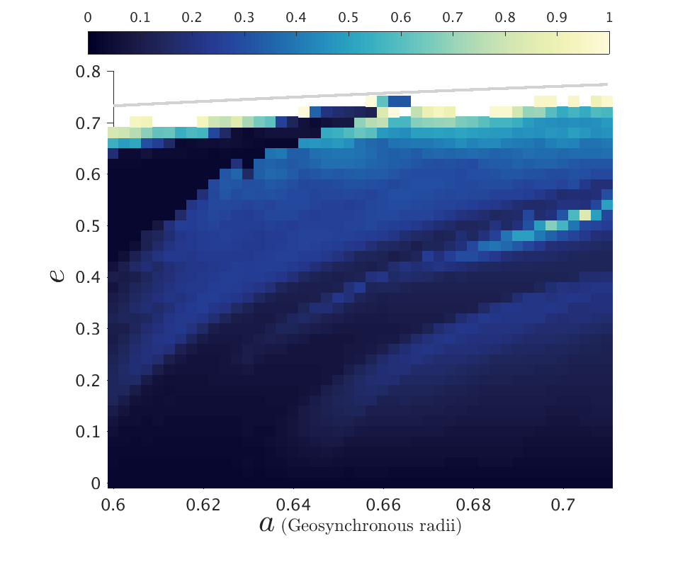
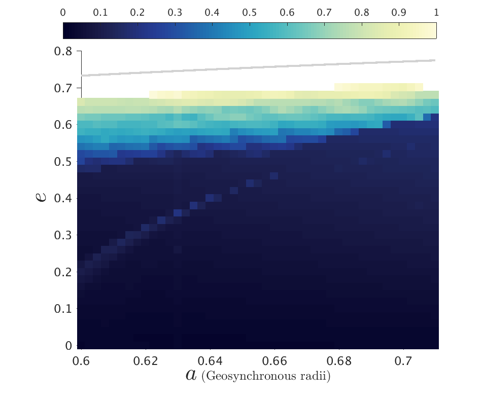
(d) $\bm{i}_{o}={\bf 46^{\circ}}$

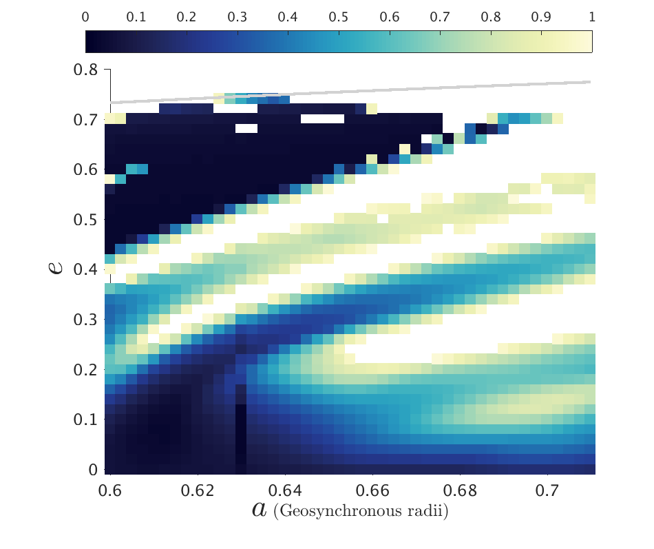
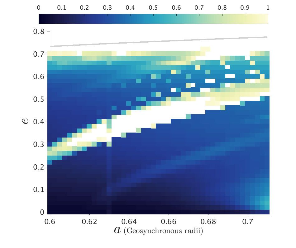
(e) $\bm{i}_{o}={\bf 54^{\circ}}$

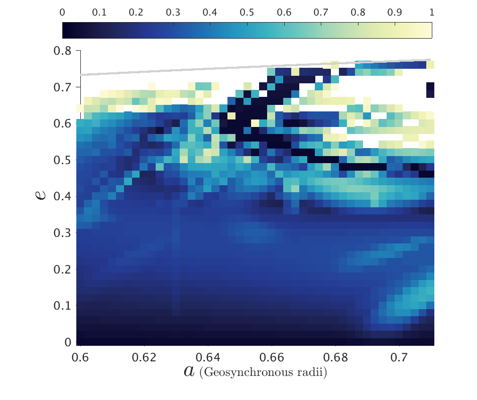
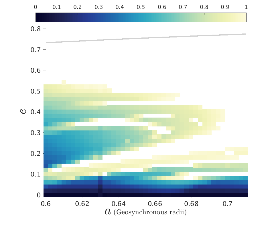
(f) $\bm{i}_{o}={\bf 58^{\circ}}$

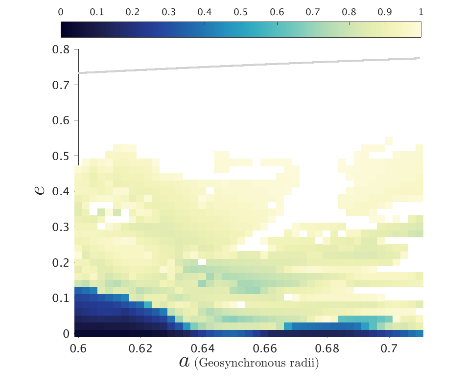
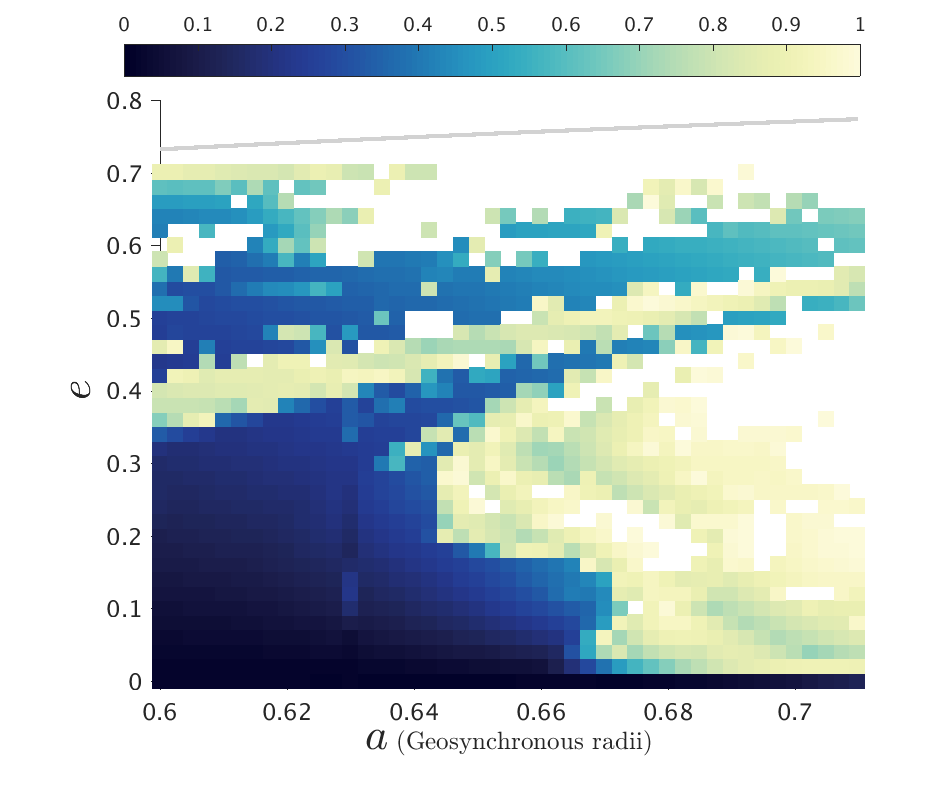
(g) $\bm{i}_{o}={\bf 66^{\circ}}$

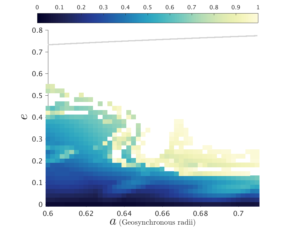
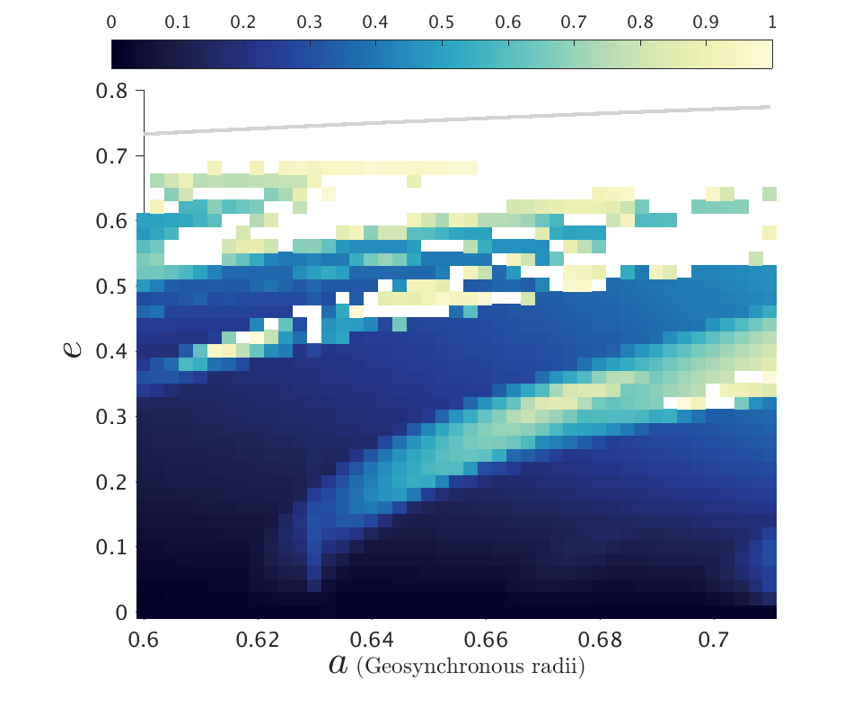
(h) $\bm{i}_{o}={\bf 68^{\circ}}$

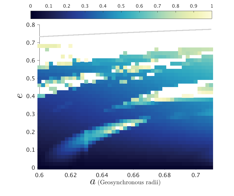
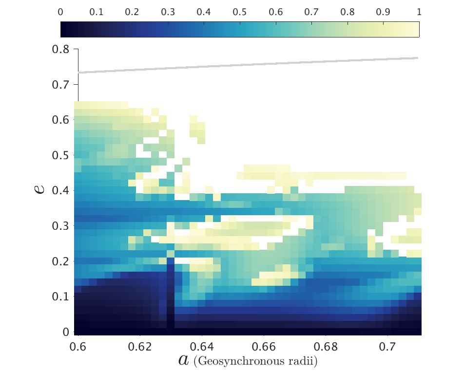
(i) $\bm{i}_{o}={\bf 70^{\circ}}$

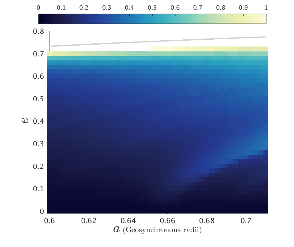
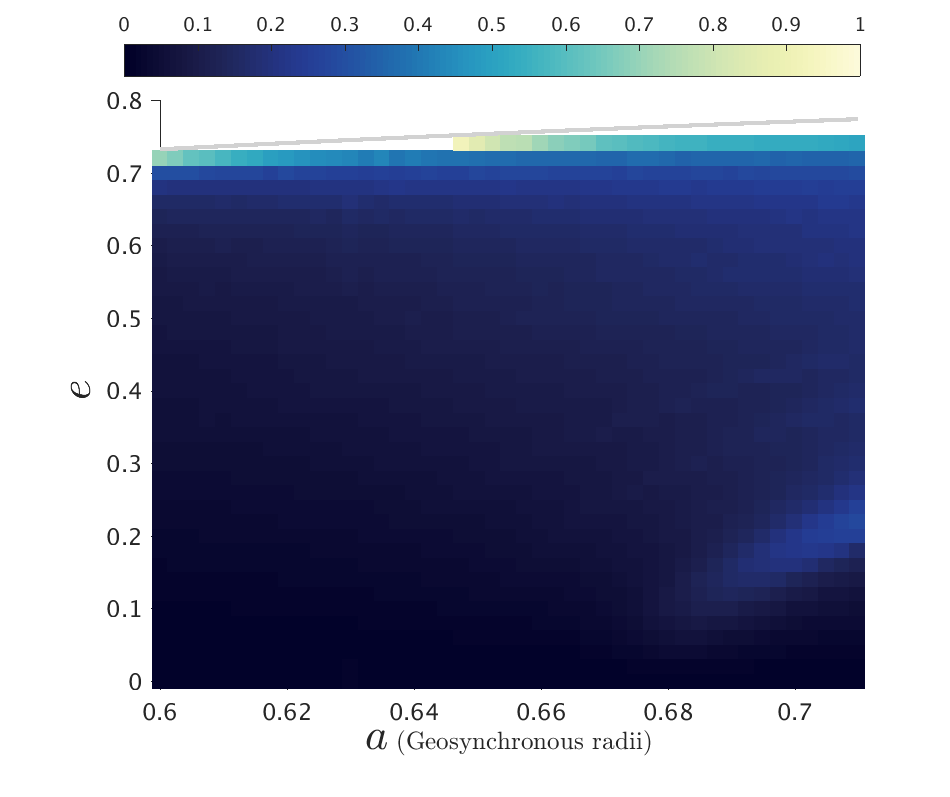
(j) $\bm{i}_{o}={\bf 90^{\circ}}$

Figure 20: $De$ maps of the MEO-general phase space for various $\bm{i}_{o}$, $\bm{\Delta}\bm{\Omega}={\bf 180^{\circ}}$, $\bm{\Delta}\bm{\omega}={\bf 270^{\circ}}$ (1st and 3rd columns) and $\bm{\Delta}\bm{\Omega}={\bf 270^{\circ}}$, $\bm{\Delta}\bm{\omega}={\bf 90^{\circ}}$ (2nd and 4th columns), for Epoch 2018, and for $C_{R}A/m=1$ m²/kg. The colorbar for the $De$ maps is from 0 to 1, where the reentry particles were excluded (white).

(a) $\bm{i}_{o}={\bf 0}$

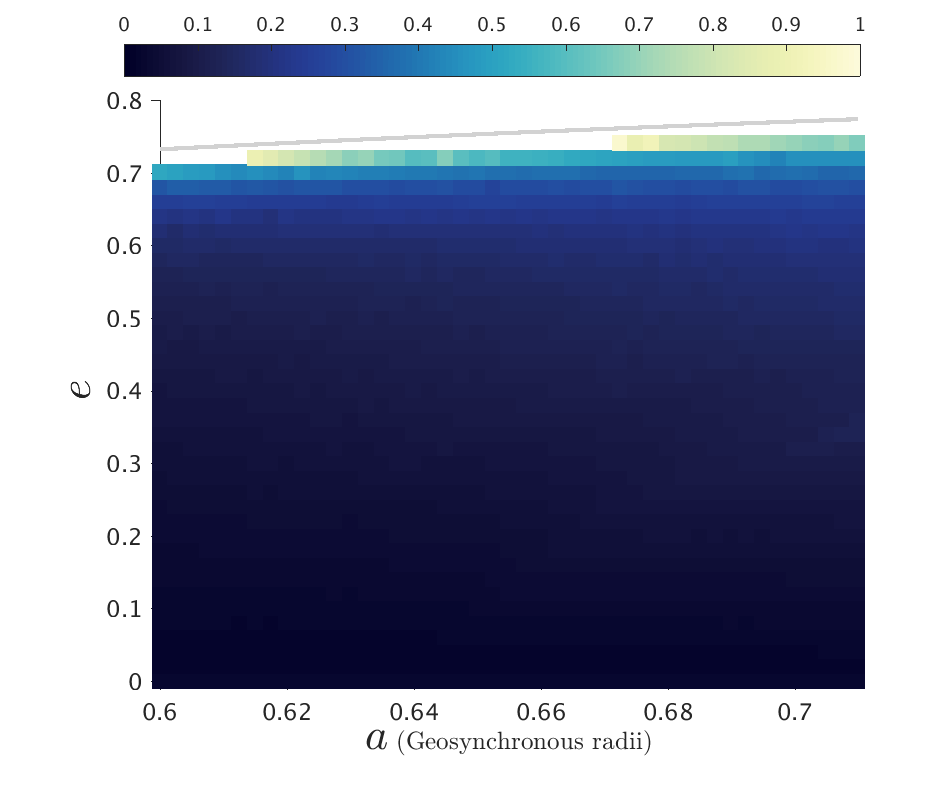
(b) $\bm{i}_{o}={\bf 28^{\circ}}$

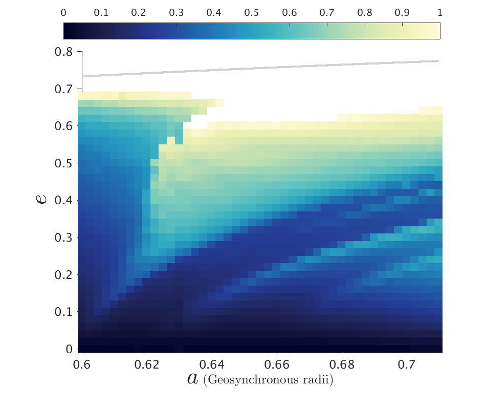
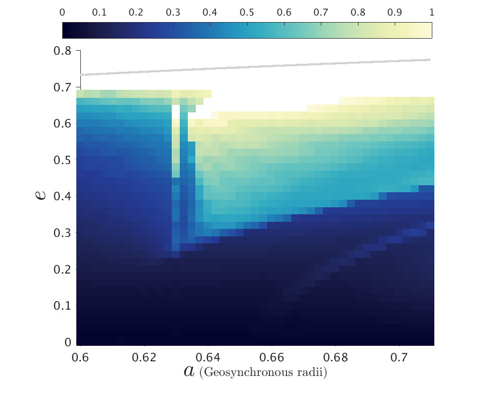
(c) $\bm{i}_{o}={\bf 44^{\circ}}$

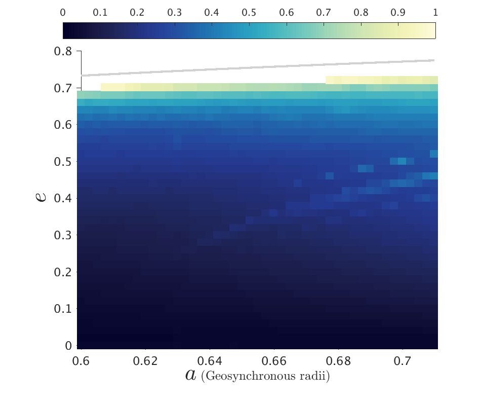
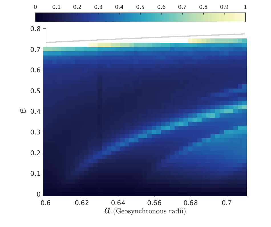
(d) $\bm{i}_{o}={\bf 46^{\circ}}$

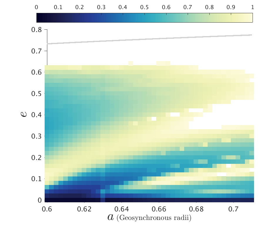
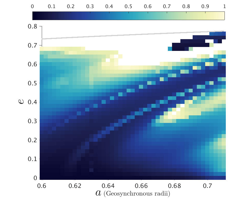
(e) $\bm{i}_{o}={\bf 54^{\circ}}$

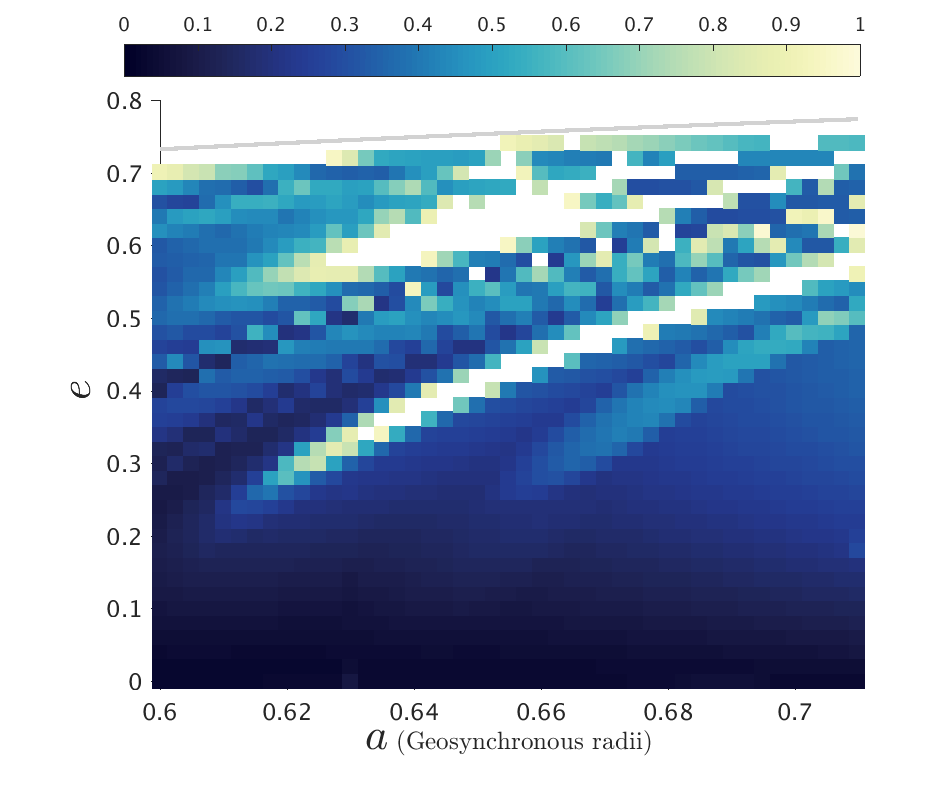
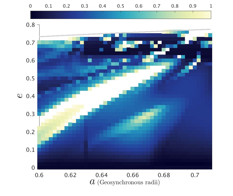
(f) $\bm{i}_{o}={\bf 58^{\circ}}$

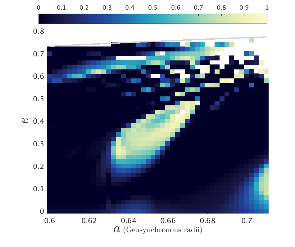
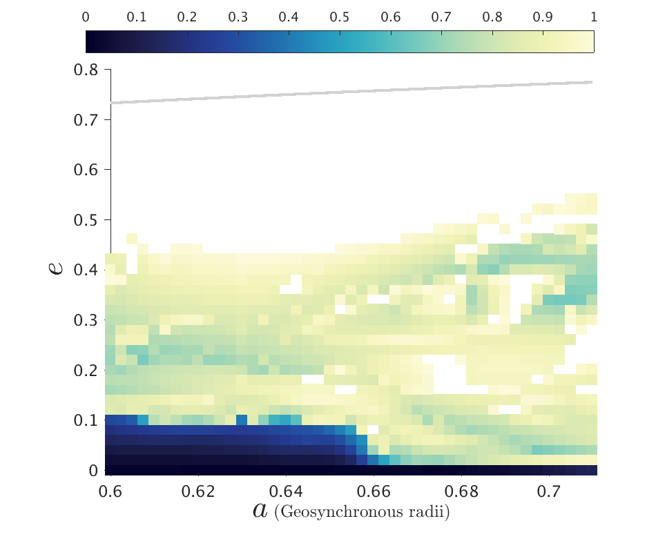
(g) $\bm{i}_{o}={\bf 66^{\circ}}$

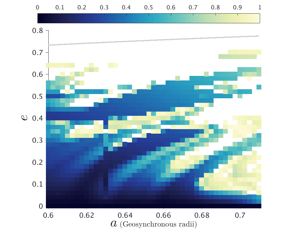
(h) $\bm{i}_{o}={\bf 68^{\circ}}$

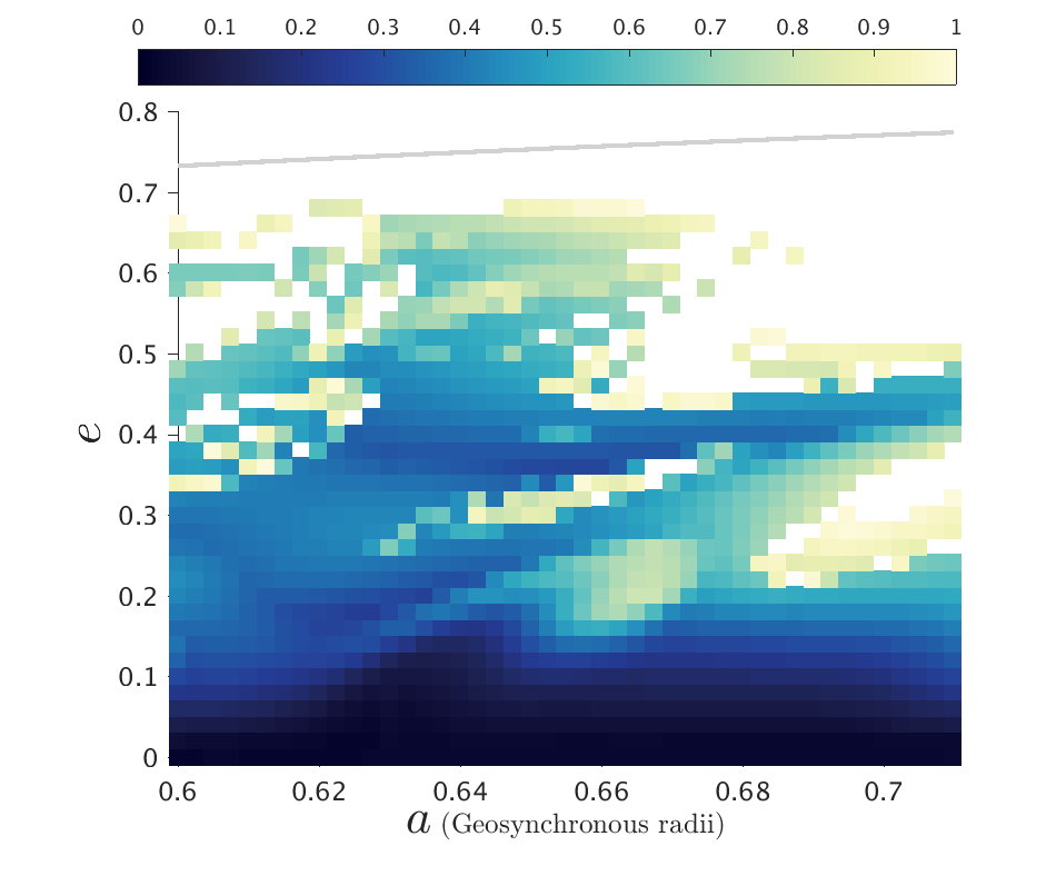
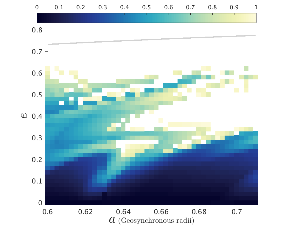
(i) $\bm{i}_{o}={\bf 70^{\circ}}$

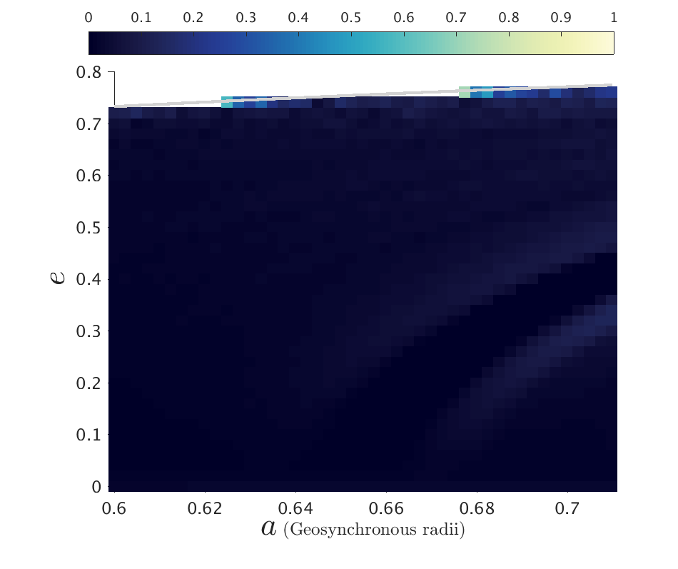
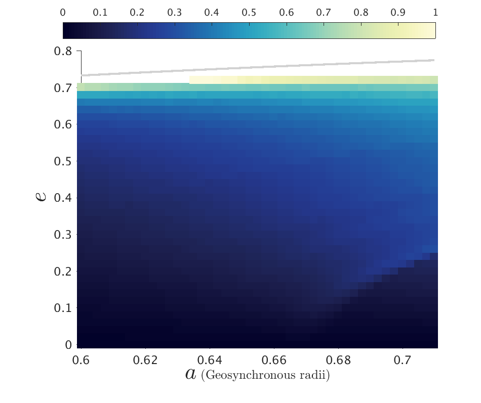
(j) $\bm{i}_{o}={\bf 90^{\circ}}$

Figure 21: $De$ maps of the MEO-general phase space for various $\bm{i}_{o}$, $\bm{\Delta}\bm{\Omega}={\bf 180^{\circ}}$, $\bm{\Delta}\bm{\omega}={\bf 270^{\circ}}$ (1st and 3rd columns) and $\bm{\Delta}\bm{\Omega}={\bf 270^{\circ}}$, $\bm{\Delta}\bm{\omega}={\bf 90^{\circ}}$ (2nd and 4th columns), for Epoch 2020, and for $C_{R}A/m=1$ m²/kg. The colorbar for the $De$ maps is from 0 to 1, where the reentry particles were excluded (white).

Appendix B Dynamical maps of GNSS-graveyard grid for $i_{nom}-0.5^{\circ}$ and $i_{nom}+0.5^{\circ}$

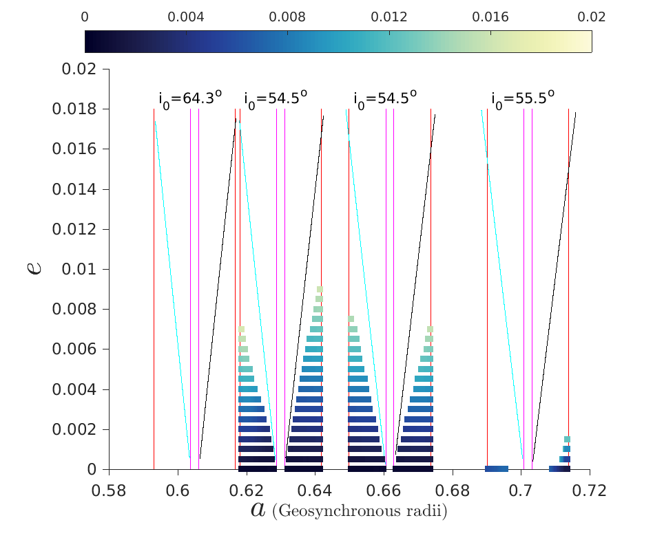
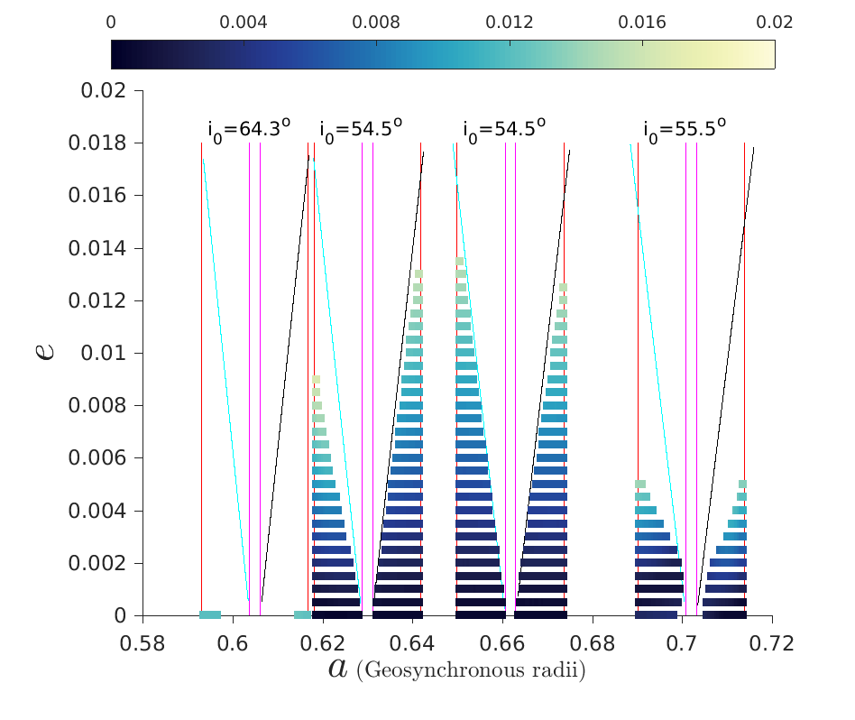
(a) $\bm{\Delta}\bm{\Omega}={\bf 0}$, $\bm{\Delta}\bm{\omega}={\bf 0}$

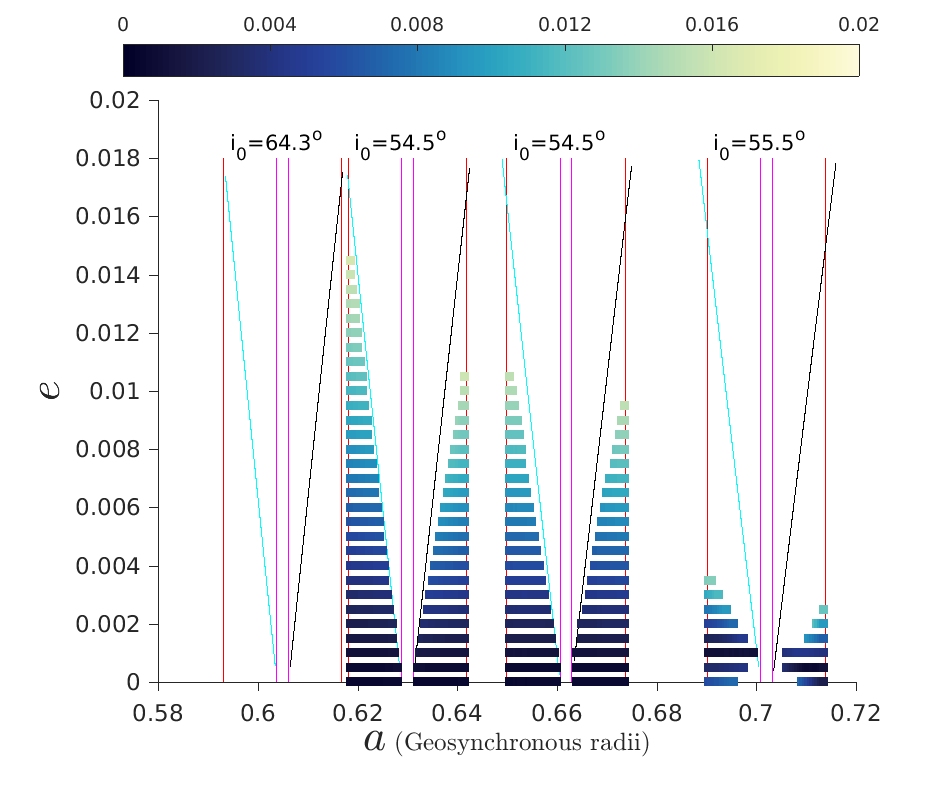
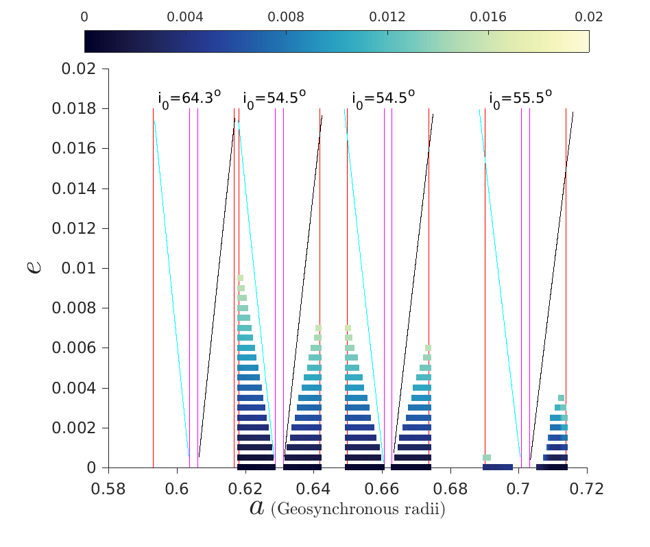
(b) $\bm{\Delta}\bm{\Omega}={\bf 0}$, $\bm{\Delta}\bm{\omega}={\bf 90^{\circ}}$

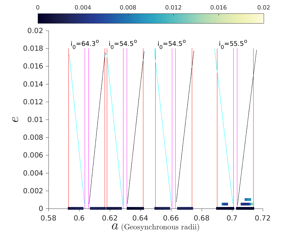
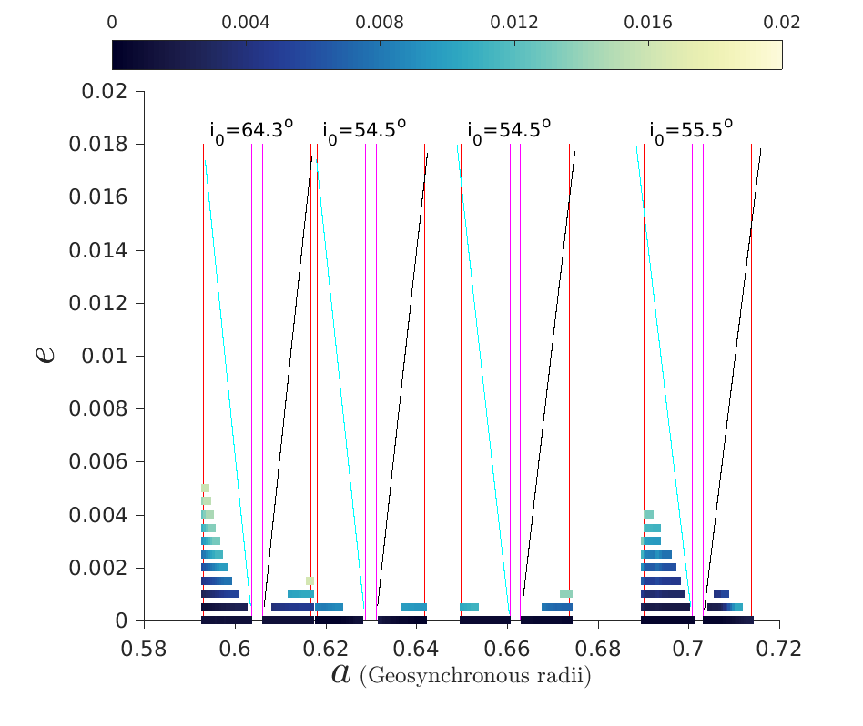
(c) $\bm{\Delta}\bm{\Omega}={\bf 90^{\circ}}$, $\bm{\Delta}\bm{\omega}={\bf 0}$

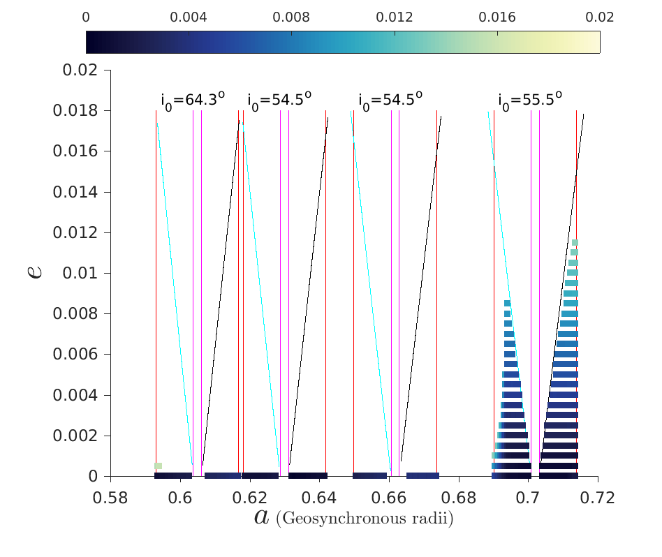
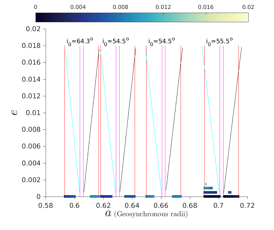
(d) $\bm{\Delta}\bm{\Omega}={\bf 90^{\circ}}$, $\bm{\Delta}\bm{\omega}={\bf 90^{\circ}}$

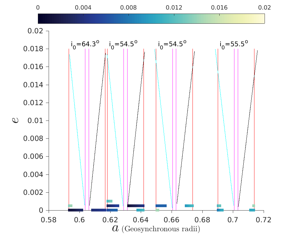
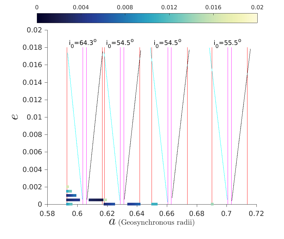
(e) $\bm{\Delta}\bm{\Omega}={\bf 180^{\circ}}$, $\bm{\Delta}\bm{\omega}={\bf 0}$

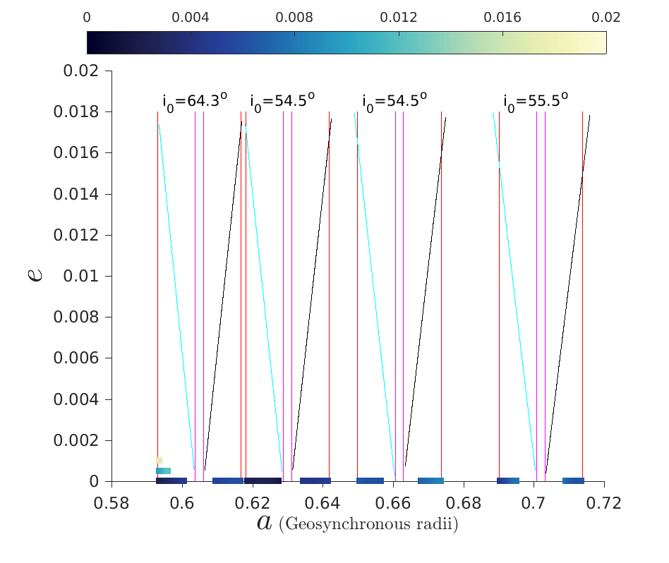
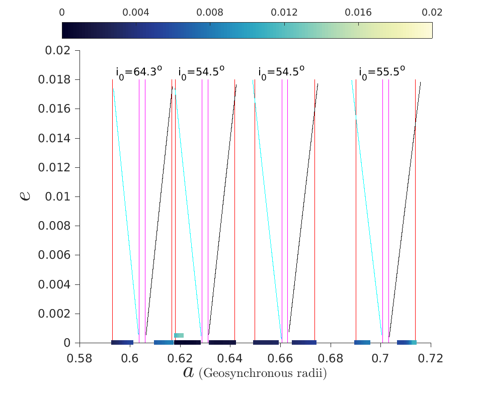
(f) $\bm{\Delta}\bm{\Omega}={\bf 180^{\circ}}$, $\bm{\Delta}\bm{\omega}={\bf 90^{\circ}}$

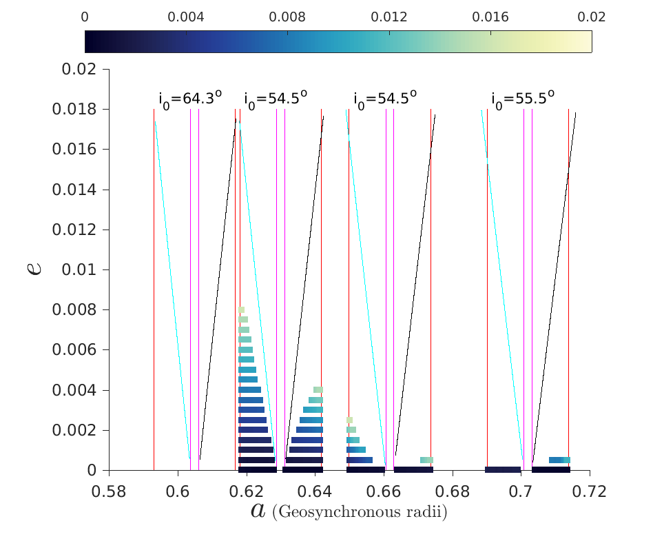
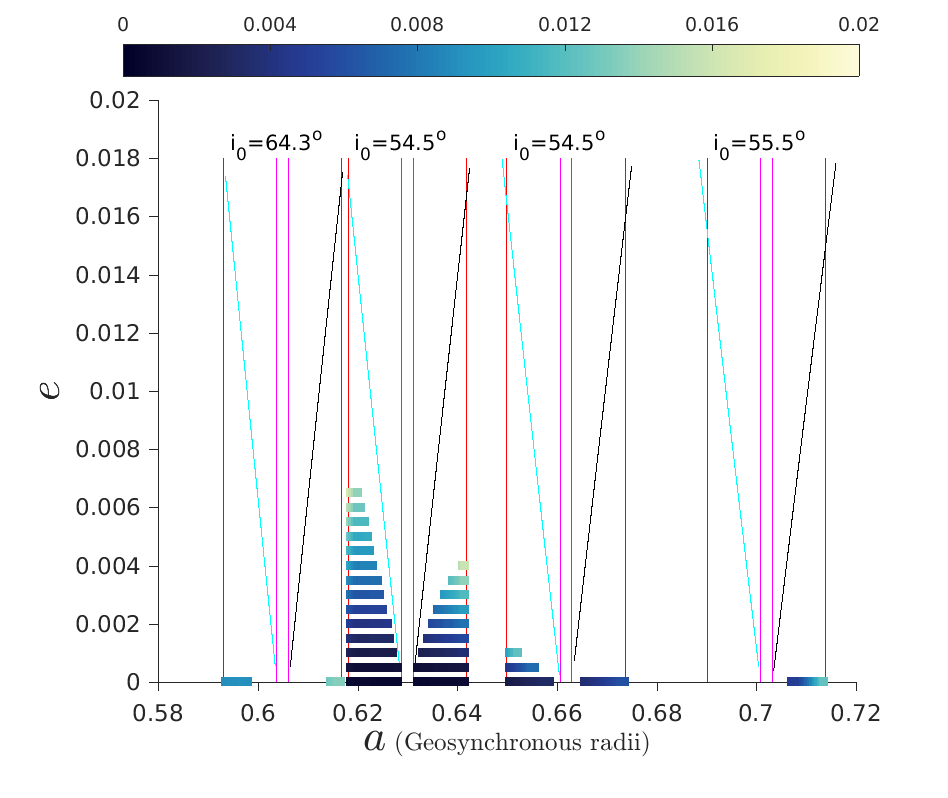
(g) $\bm{\Delta}\bm{\Omega}={\bf 270^{\circ}}$, $\bm{\Delta}\bm{\omega}={\bf 0}$

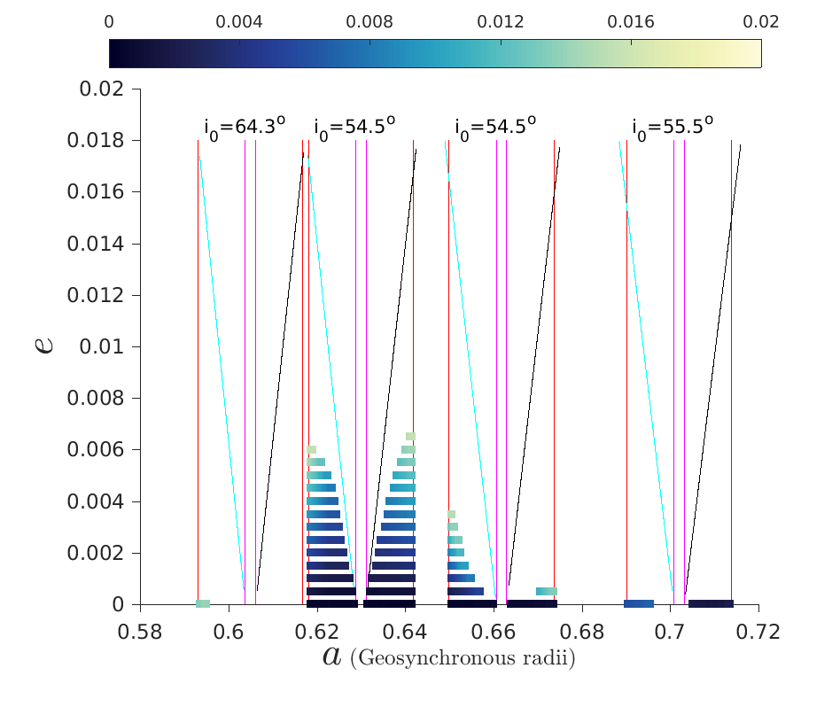
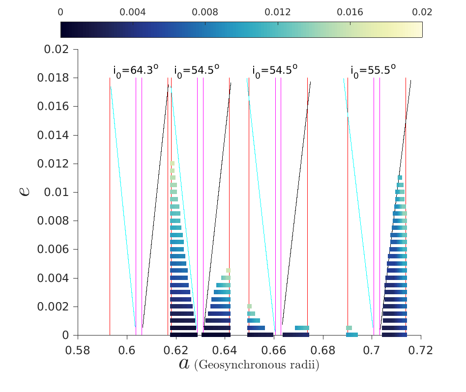
(h) $\bm{\Delta}\bm{\Omega}={\bf 270^{\circ}}$, $\bm{\Delta}\bm{\omega}={\bf 90^{\circ}}$

Figure 22: Maximum eccentricity maps of the GNSS-graveyard phase space for $\bm{i_{o}}={\bf i_{nom}-0.5^{\circ}}$, for Epoch 2018 (left) and Epoch 2020 (right), and for $C_{R}A/m=0.015$ m²/kg. $i=64.3^{\circ}$ for GLONASS, $54.5^{\circ}$ for GPS and BEIDOU, and $55.5^{\circ}$ for GALILEO. The colorbar for maximum eccentricity maps is from 0 to 0.02.

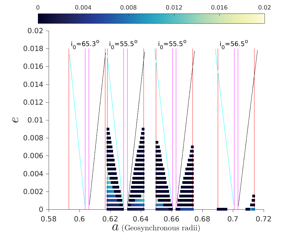
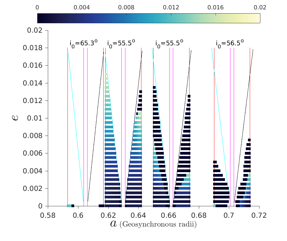
(a) $\bm{\Delta}\bm{\Omega}={\bf 0}$, $\bm{\Delta}\bm{\omega}={\bf 0}$

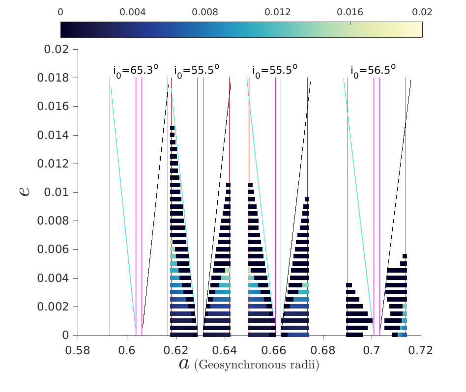
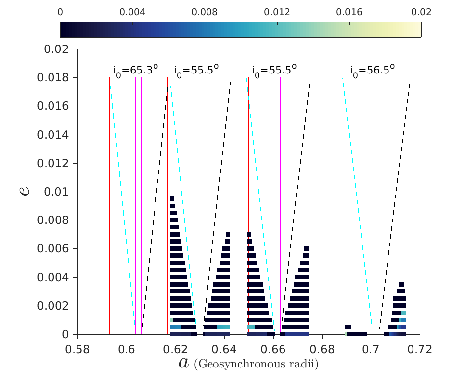
(b) $\bm{\Delta}\bm{\Omega}={\bf 0}$, $\bm{\Delta}\bm{\omega}={\bf 90^{\circ}}$

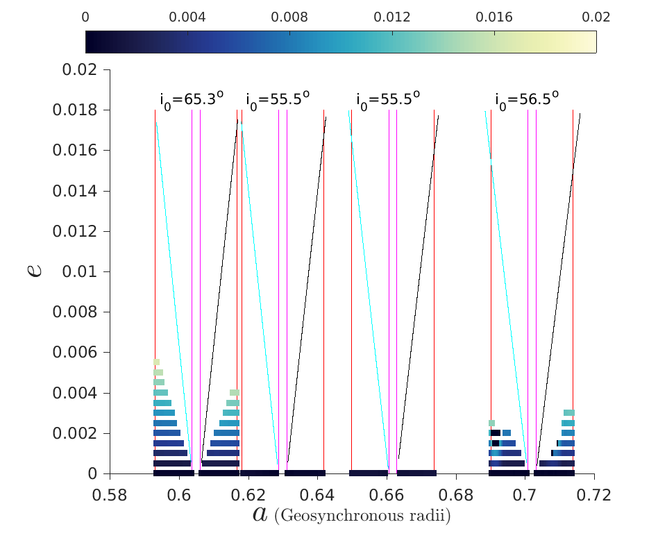
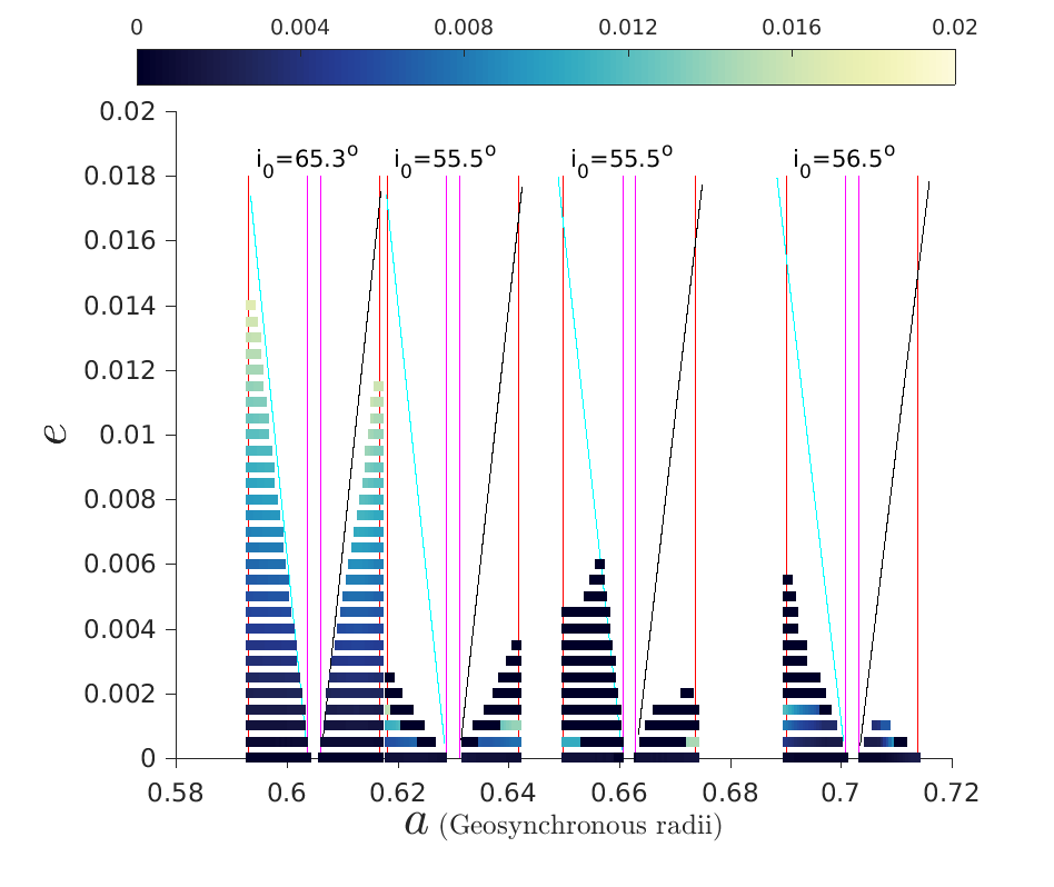
(c) $\bm{\Delta}\bm{\Omega}={\bf 90^{\circ}}$, $\bm{\Delta}\bm{\omega}={\bf 0}$

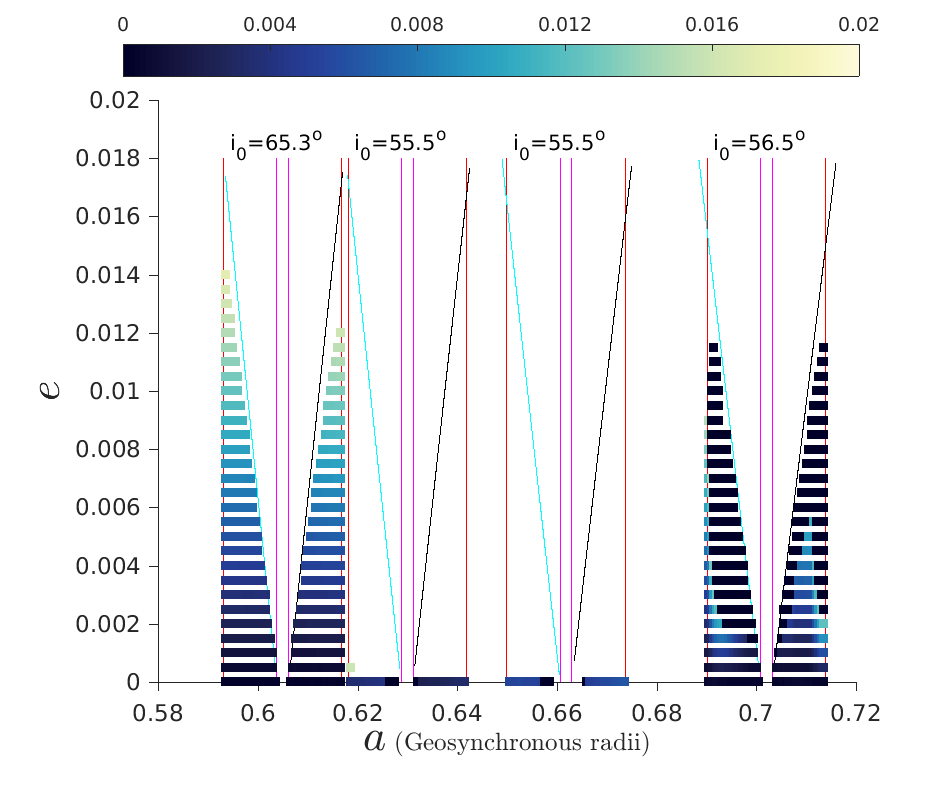
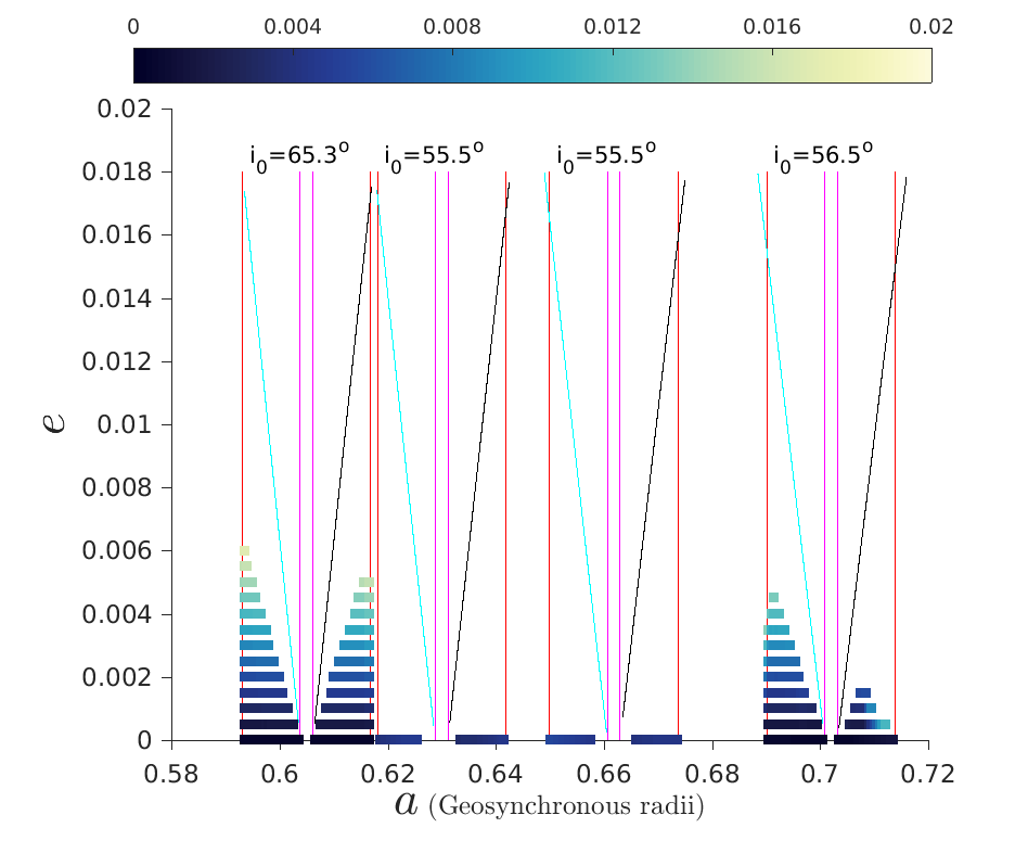
(d) $\bm{\Delta}\bm{\Omega}={\bf 90^{\circ}}$, $\bm{\Delta}\bm{\omega}={\bf 90^{\circ}}$

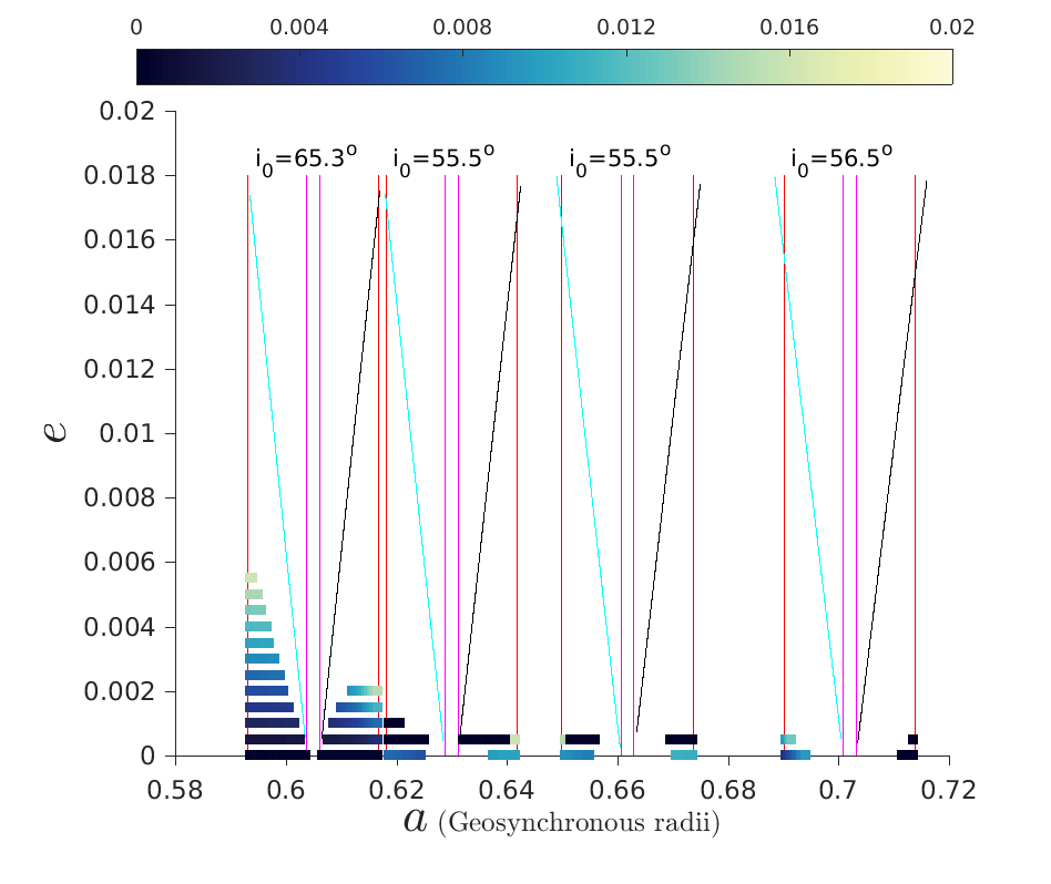
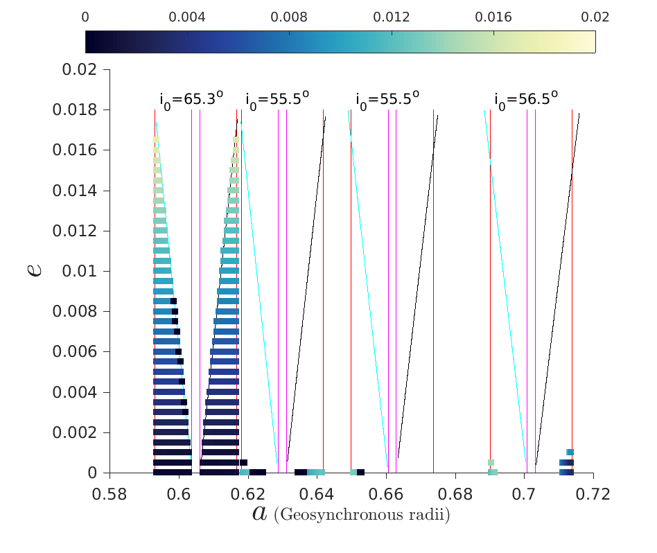
(e) $\bm{\Delta}\bm{\Omega}={\bf 180^{\circ}}$, $\bm{\Delta}\bm{\omega}={\bf 0}$

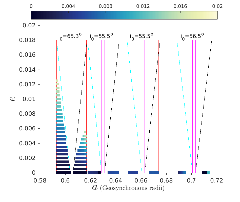
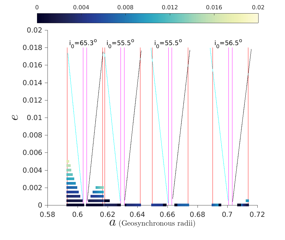
(f) $\bm{\Delta}\bm{\Omega}={\bf 180^{\circ}}$, $\bm{\Delta}\bm{\omega}={\bf 90^{\circ}}$

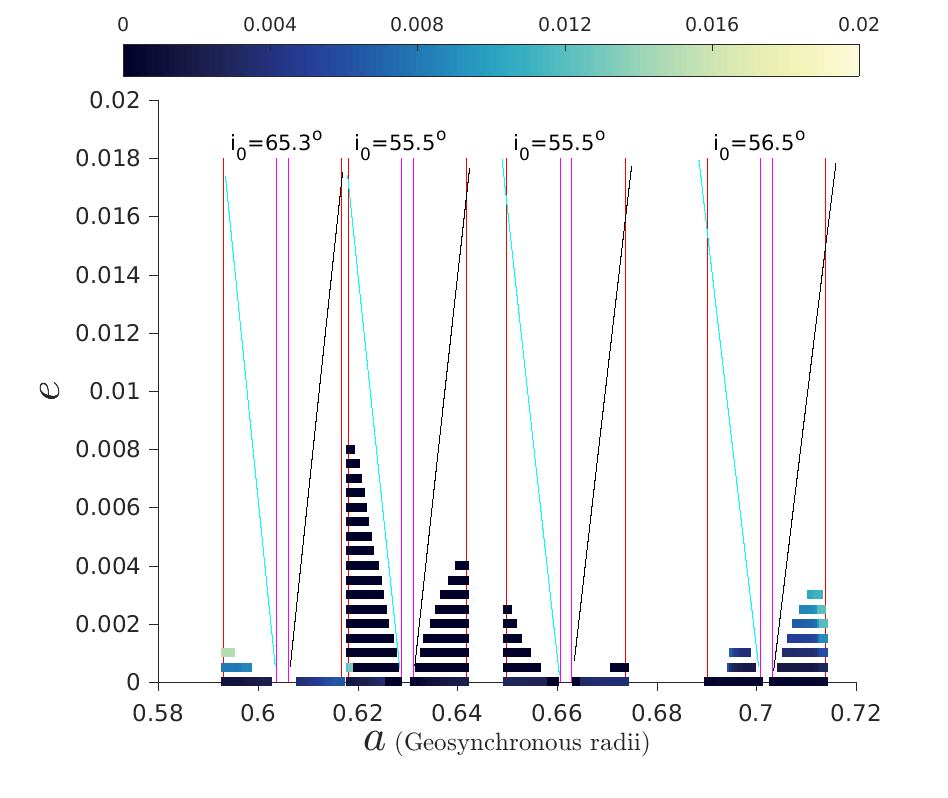
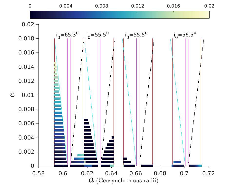
(g) $\bm{\Delta}\bm{\Omega}={\bf 270^{\circ}}$, $\bm{\Delta}\bm{\omega}={\bf 0}$

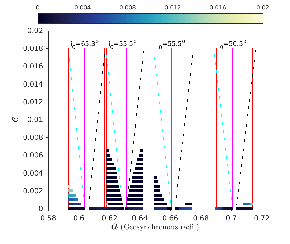
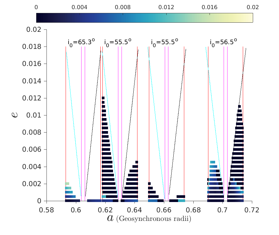
(h) $\bm{\Delta}\bm{\Omega}={\bf 270^{\circ}}$, $\bm{\Delta}\bm{\omega}={\bf 90^{\circ}}$

Figure 23: Maximum eccentricity maps of the GNSS-graveyard phase space for $\bm{i_{o}}={\bf i_{nom}+0.5^{\circ}}$, for Epoch 2018 (left) and Epoch 2020 (right), and for $C_{R}A/m=0.015$ m²/kg. $i=65.3^{\circ}$ for GLONASS, $55.5^{\circ}$ for GPS and BEIDOU, and $56.5^{\circ}$ for GALILEO. The colorbar for maximum eccentricity maps is from 0 to 0.02.

References

- Alessi et al. (2016) Alessi, E. M., Deleflie, F., Rosengren, A.J., Rossi A., Valsecchi , G. B., Daquin J., Merz K, 2016. A numerical investigation on the eccentricity growth of GNSS disposal orbits. Celestial Mech. Dyn. Astron. 125, 71–90.
- Alessi et al. (2018a) Alessi, E.M., Schettino, G., Rossi, A., Valsecchi, G.B., 2018a. Solar radiation pressure resonances in Low Earth Orbits. Mon. Not. R. Astron. Soc. 473, 2407–2414.
- Alessi et al. (2018b) Alessi, E.M., Schettino, G., Rossi, A., Valsecchi, G.B., 2018b. Natural Highways for End-of-Life Solutions in the LEO Region. Celestial Mech. Dyn. Astron. 130, 34–55.
- Armellin and San-Juan (2018) Armellin, R., San-Juan, J. F., 2018. Optimal Earth’s reentry disposal of Galileo constellation. Adv. Space Res. 61(4), 1097–1120.
- Breiter (2001) Breiter, S., 2001b. Lunisolar resonances revisited. Celestial Mech. Dyn. Astron. 81, 81–91.
- Celletti and Galeş (2016) Celletti A., Galeş C., 2016. A study of the lunisolar secular resonance . Frontiers in Astronomy and Space Sciences, 3, 11.
- Chao (2000) Chao C., 2000. MEO disposal orbit stability and direct reentry strategy. In: Proceedings of the AAS/AIAA Space Flight Mechanics Meeting, Clearwater, FL, paper AAS No. 00-152.
- Colombo and Gkolias (2017) Colombo, C., Gkolias, I., 2017. Analyis of Orbit stability in the Geosynchronous region for End-Of-Life disposal. In: Proceedings of the 7th European Conference on Space Debris, Darmstadt, Germany.
- Cook (1962) Cook, G.E., 1962. Luni-Solar Perturbations of the Orbit of an Earth Satellite. The Geophysical Journal of the Royal Astronomical Society 6(3), 271–291.
- Daquin et al. (2015) Daquin, J., Deleflie, F., Pérez, J., 2015. Comparison of mean and osculating stability in the vicinity of the (2:1) tesseral resonant surface. Acta Astronaut. 111, 170–177.
- Daquin et al. (2016) Daquin, J., Rosengren, A.J., Alessi, E.M., Deleflie, F., Valsecchi , G.B., Rossi, A., 2016. The dynamical structure of the MEO region: long-term stability, chaos, and transport. Celestial Mech. Dyn. Astron. 124, 335–366.
- Gkolias et al. (2016) Gkolias, I., Daquin, J., Gachet, F., Rosengren, A.J., 2016. From order to chaos in Earth satellite orbits. Astron. J. 152, 119–133.
- Gkolias and Colombo (2017) Gkolias, I., Colombo, C., 2017. End-of-Life Disposal of Geosynchronous Satellites. International Astronautical Congress 2017, 25-29 September 2017, Adelaide, Australia
- Gobetz and Doll (1969) Gobetz, F.W., Doll, J.R., 1969. A survey of impulsive trajectories AIAA J. 7, 801–834.
- Holzinger et al. (2014) Holzinger, M.J.., Scheeres, D.J., Erwin, R.S., 2014. On-orbit operational range computations using Gauss’s variational equations with perturbations. J. Guid. Cont. Dyn. 37, 608–622.
- Jenkin and Gick (2005) Jenkin, A. B., Gick, R. A., 2005. Dilution of disposal orbit collision risk for the medium Earth orbit constellations. In: Proceedings of the 4th European Conference on Space Debris, Darmstadt, Germany.
- Levison and Duncan (1994) Levison, H.F., Duncan, M.J., 1994. The long-term dynamical behavior of short-period comets. Icarus. 108, 18–36.
- Marec (1979) Marec, J.-P., 1979. Optimal Space Trajectories. Amsterdam, Elsevier Scientific.
- McInnes (1999) McInnes, C.R., 1999. Solar Sailing: Technology, Dynamics and Mission Applications. Berlin, Springer-Verlag.
- Mistry and Armellin (2016) Mistry D, Armellin R., 2016. The Design and Optimisation of End-of-Life Disposal Manoeuvres for GNSS Spacecraft: The Case of Galileo. In: Proceedings of the 66th International Astronautical Congress, 2015 3 pp. 2187–2199.
- Radtke et al. (2015) Radtke, J., Domnguez-Gonzales, R., Flegel, S.K., Snchez-Ortiz, N., Merz, K., 2015. Impact of eccentricity build-up and graveyard disposal strategies on MEO navigation constellations. Adv. Space Res. 56(11), 2626–2644.
- Rosengren et al. (2015) Rosengren, A.J. Alessi, E.M., Rossi, A., Valsecchi, G.B., 2015. Chaos in navigation satellite orbits caused by the perturbed motion of the Moon. Mon. Not. R. Astron. Soc. 464, 3522–3526.
- Rosengren et al. (2017) Rosengren, A.J., Daquin, J., Tsiganis, K., et al., 2017. Galileo disposal strategy: stability, chaos and predictability. Mon. Not. R. Astron. Soc. 449, 4063–4076.
- Rosengren et al. (2019) Rosengren, A.J., Skoulidou D.K., Tsiganis K., Voyatzis G., 2019. Dynamical cartography of Earth satellite orbits. Adv. Space Res. 63(1), 443–460.
- Rossi (2008) Rossi, A., 2008. Resonant dynamics of medium Earth orbits: space debris issues. Celestial Mech. Dyn. Astron., 100, 267–286.
- Rossi et al. (2018) Rossi, A., and the ReDSHIFT team, 2018. ReDSHIFT: a global approach to space debris mitigation. Aerospace 2018, 5, 64–78.
- Sidi (1997) Sidi, M.J., 1997. Spacecraft Dynamics & Control: A Practical Engineering Approach. New York, Cambridge University Press.
- Skoulidou et al. (2017) Skoulidou, D.K., Rosengren, A.J., Tsiganis, K., Voyatzis, G., 2017. Cartographic study of the MEO phase space for passive debris removal. In: Proceedings of the 7th European Conference on Space Debris, Darmstadt, Germany.
- Skoulidou et al. (2018) Skoulidou, D.K., Rosengren, A.J., Tsiganis, K., Voyatzis, G., 2018. Dynamical lifetime survey of geostationary transfer orbits. Celestial Mech. Dyn. Astron., 130, 77–94.
- Stefanelli and Metris (2015) Stefanelli, E., Metris, G., 2015. Solar gravitational perturbations on the dynamics of MEO: increase of the eccentricity due to resonances. Adv. Space Res. 55(7), 1855–1867.
- Wisdom and Holman (1991) Wisdom, J., Holman, M., 1991. Symplectic maps for the N-body problem. Astron. J. 102, 1528–1538.
- Xue et al. (2010) Xue, D., Li, J., Baoyin, H., Jiang, F., 2010. Reachable domain for spacecraft with single impulse. J. Guid. Cont. Dyn. 33, 934–942.