On the Displacement of Eigenvalues when Removing a Twin Vertex

Abstract

Twin vertices of a graph have the same open neighbourhood. If they are not adjacent, then they are called duplicates and contribute the eigenvalue zero to the adjacency matrix. Otherwise they are termed co-duplicates, when they contribute $-1$ as an eigenvalue of the adjacency matrix. On removing a twin vertex from a graph, the spectrum of the adjacency matrix does not only lose the eigenvalue $0$ or $-1$. The perturbation sends a rippling effect to the spectrum. The simple eigenvalues are displaced. We obtain a closed formula for the characteristic polynomial of a graph with twin vertices in terms of two polynomials associated with the perturbed graph. These are used to obtain estimates of the displacements in the spectrum caused by the perturbation.

[On the Displacement of Eigenvalues] 05C50 Johann A. BriffaJ.A.Briffa Department of Communications and Computer Engineering
University of Malta, Msida MSD 2080, Malta [johann.briffa@um.edu.mt] Irene ScirihaI.Sciriha Department of Mathematics
University of Malta, Msida MSD 2080, Malta [irene.sciriha-aquilina@um.edu.mt]

1 Introduction

We limit ourselves to simple connected graphs, that is graphs with no multiple edges or loops. A graph $G(V,E)$ has a vertex set $V=\{1,2,\ldots,n\}$ and an edge set $E$ whose elements are distinct pairs of vertices of $V$. The set $\overline{E}$ of non-edges of $G$ are those pairs of distinct vertices not in $E$. The complement $\overline{G}(V,\overline{E})$ of $G$ has the same vertex set as $G$ and edge set $\overline{E}$. Twin vertices are either duplicate or co-duplicate. Two vertices are called duplicate if they are non-adjacent and have the same neighbours. A pair of co-duplicate vertices in a graph $G$ are adjacent, and they are duplicate vertices in the complement $\overline{G}$.

Let $\mathbf{A}(G)$, also written as $\mathbf{A}=(a_{i,j})$, be the adjacency matrix of $G$ with $a_{i,j}=1$ if the vertices $i,j$ are adjacent and zero otherwise. The eigenvalues of $\mathbf{A}$ are referred to as the eigenvalues of $G$ and form the spectrum of $G$. If $G$ has a pair of duplicate vertices, then the corresponding rows (and columns) in $\mathbf{A}$ are the same. This means that $\mathbf{A}$ has the eigenvalue zero. In the case where $G$ has two co-duplicate vertices, the corresponding rows and columns are the same except for the two entries defining the edge between them. This means that $-1$ is in the spectrum of $G$. In both cases the associated eigenvector has two non-zero entries.

Unlike what one may assume, removing a twin vertex does not just remove the eigenvalue $0$ or $-1$ in the respective cases, while preserving the rest of the spectrum. Indeed, we investigate the shift in eigenvalues on removing a twin vertex. To calculate the new eigenvalues after removing a twin vertex, one has to perform the computation on the adjacency matrix of the new graph, ignoring any information known about the original graph. In this work, we provide ways to directly calculate estimates for the changes in eigenvalues, as a difference from those of the original graph. We also give an explicit expression for the change in the characteristic polynomial due to the removal of a twin vertex.

While to our knowledge this specific problem has not been treated before, the literature on spectral graph theory contains a number of related works. In the 1950s, Heilbronner derived the characteristic polynomial of a perturbed graph from that of the parent graph. He determined explicitly the eigenvalues of the subgraph on deleting a vertex from a graph, contributing to the study of molecular orbitals [1, 2, 3, 4, 5]. Later, in the literature, one finds expressions for the characteristic polynomial of an arbitrary graph, of graphs with particular geometric properties and of perturbed graphs also in the work of Schwenk [6] and Rosenfeld [7].

The well known Cauchy inequalities, involving the eigenvalues of a real symmetric matrix and a principal submatrix, are referred to as the interlacing theorem in spectral graph theory [6]. The theorem states that exactly one root of the characteristic polynomial of a vertex deleted graph lies between two successive eigenvalues of the parent graph. It was the subject of many studies by the pioneers in the theory of the matrices that encode the structure of a graph. Its application unlocked many remarkable latent properties of classes of graphs. Interlacing is the main tool used by Thüne in his PhD thesis [8] to determine certain substructures in graphs.  Later, Haemers produced a survey [9] of the various kinds of applications of eigenvalue interlacing to complement his doctoral thesis [10]. More recently, Lovász emphasised the importance of interlacing and gave a summary of the main results on the eigenvalues of matrices of a graph [11]. In a collaboration with Simić, Marino et al. used the interlacing theorem to explore the properties of line graphs of trees with twin vertices deleted [12]. Sciriha et al. studied classes of graphs that showed the largest possible change in the multiplicity of the eigenvalue zero as a consequence of interlacing [13]. An independent set is a subset of the vertices such that no two of the vertices are adjacent. One of the graph invariants that is widely studied in combinatorics is the independence number, that is the size of the largest independent set. Rowlinson, a main exponent of graph eigenvalues, finds bounds on the independence number of a graph basing his arguments on interlacing [14].

Sciriha and Farrugia consider the threshold graph which is a split graph in which the vertex set is partitioned into an independent set and a clique, which is a subset of the vertices that induces a complete subgraph in which every two vertices are adjacent [15]. The independent set may contain duplicates and the clique may contain co-duplicates. Mohammadian and Trevisan show that there are no eigenvalues of the adjacency matrix of a threshold graph between $0$ and $-1$, which in threshold graphs are contributed only by twin vertices [16].

The interlacing theorem applies to all the real symmetric matrices encoding $G$, including the Laplacian matrix. When considering the Laplacian, So proved that only one of its eigenvalues is displaced when an edge is added between two duplicate vertices to produce a co-duplicate [17]. The rest of the eigenvalues remain unchanged.

The interlacing theorem provides rough bounds for the displacement of the eigenvalues of $G$ when a vertex is deleted. Our objective is to obtain better estimates within these bounds. To this end, relations of $\mathop{\phi}\left(\mathbf{A}(G),\lambda\right)$ to polynomials of other submatrices of $\mathbf{A}$ are obtained. These results would be of interest in any application where the displacement in eigenvalues is of greater interest than the eigenvalues of the modified graph.

The rest of the paper is organised as follows. In Section 2, we apply similarity operations on the adjacency matrix of $G$, so that eigenvalues are preserved, to yield a matrix whose characteristic polynomial is easily expressed in terms of those of subgraphs of $G$. In Section 3, we show how the expressions obtained enable the computation of estimates of the displacement of the eigenvalues of the adjacency matrix on removing a twin vertex. Finally, we give examples of computing the estimates of the displacement of the spectrum on removing a twin vertex from a nested split graph in Appendix A, and from a general graph in Appendix B.

2 Effect on the Characteristic Polynomial on Removing a Twin Vertex

To obtain the eigenvalues of a matrix $\mathbf{M}$, it suffices to determine the roots of its characteristic polynomial $\mathop{\phi}\left(\mathbf{M},\lambda\right)$. If $\mathbf{M}$ is known to be real and symmetric, then its algebraic properties allow alternative methods of computation with possibly lower complexity. The Jacobi-Givens method [18] employs rotation of two axes of $\mathbb{R}^{n}$ to introduce zero entries in a row of $\mathbf{M}$ via a similarity operation and therefore without altering the eigenvalues. The new form of the matrix allows the characteristic polynomials of $\mathbf{M}$ and of other principal submatrices of $\mathbf{M}$ to be easily related.

Definition ((Adjacency matrix)).

The adjacency matrix $\mathbf{A}$ of a graph $G$ of order $n$, where the two first labelled vertices $v_{1}$,$v_{2}$ are twin vertices, can be written as

(1) $$\mathbf{A}=\left(\begin{array}[]{cc|c}0&a&\mathbf{b}^{\top}\\ a&0&\mathbf{b}^{\top}\\ \hline\cr\mathbf{b}&\mathbf{b}&\mathbf{C}\end{array}\right)\text{,}$$

where $\mathbf{C}=\mathbf{A}(G_{-v_{1}-v_{2}})$ is the adjacency matrix of the subgraph $G_{-v_{1}-v_{2}}$ of $G$, obtained from $G$ by removing vertices $v_{1}$,$v_{2}$ and the edges incident to them. The entry $a$ is $0$ for duplicate and $1$ for co-duplicate vertices.

Proposition .

The adjacency matrix $\mathbf{A}$ is similar to the simpler matrix

(2) $$\mathbf{A^{\prime}}=\left(\begin{array}[]{cc|c}a&0&\sqrt{2}\mathbf{b}^{\top}\\ 0&-a&\mathbf{0}^{\top}\\ \hline\cr\sqrt{2}\mathbf{b}&\mathbf{0}&\mathbf{C}\end{array}\right)\text{.}$$

Proof.

We use the Jacobi-Givens method to find a matrix $\mathbf{P}$ such that $\mathbf{A^{\prime}}=\mathbf{P^{-1}}\mathbf{A}\mathbf{P}$. Since twin vertices have the same open neighbourhood, a rotation by $\frac{\pi}{4}$ of the corresponding axes in $\mathbb{R}^{n}$ is required. This is achieved by using

(3) $$\mathbf{P}=\left(\begin{array}[]{cc|c}\frac{1}{\sqrt{2}}&-\frac{1}{\sqrt{2}}&\mathbf{0}\\ \frac{1}{\sqrt{2}}&\frac{1}{\sqrt{2}}&\mathbf{0}\\ \hline\cr\mathbf{0}&\mathbf{0}&\mathbf{I}\end{array}\right)\text{,}$$

where $\mathbf{I}$ is the identity matrix. ∎

Corollary .

(4) $$\mathop{\phi}\left(\mathbf{A^{\prime}},\lambda\right)=\det(\lambda\mathbf{I}-\mathbf{P^{-1}}\mathbf{A}\mathbf{P})=\left|\begin{array}[]{cc|c}\lambda-a&0&-\sqrt{2}\mathbf{b}^{\top}\\ 0&\lambda+a&\mathbf{0}^{\top}\\ \hline\cr-\sqrt{2}\mathbf{b}&\mathbf{0}&\lambda\mathbf{I}-\mathbf{C}\end{array}\right|\text{.}$$

Proposition .

The characteristic polynomial of a graph $\mathbf{G}$ with adjacency matrix $\mathbf{A}$ having a pair of twin vertices is

(5) $$\mathop{\phi}\left(\mathbf{A},\lambda\right)=(\lambda^{2}-a^{2})\mathop{\phi}\left(\mathbf{C},\lambda\right)-2(\lambda+a)\mathbf{b}^{\top}\operatorname*{adj}(\lambda\mathbf{I}-\mathbf{C})\mathbf{b}\text{,}$$

where the adjugate $\operatorname*{adj}(\lambda\mathbf{I}-\mathbf{C})$ is equivalent to the expression

$$(\lambda\mathbf{I}-\mathbf{C})^{-1}\det(\lambda\mathbf{I}-\mathbf{C})\text{,}$$

for non-singular $\lambda\mathbf{I}-\mathbf{C}$.

Proof.

Using $\mathop{\phi}\left(\mathbf{A^{\prime}},\lambda\right)$ from Corollary 2 we can express the characteristic polynomial of $\mathbf{A}$ as

(6) $$\mathop{\phi}\left(\mathbf{A},\lambda\right)=\det(\lambda\mathbf{I}-\mathbf{A})=\det(\lambda\mathbf{I}-\mathbf{A^{\prime}})=(\lambda+a)\left|\begin{array}[]{c|c}\lambda-a&-\sqrt{2}\mathbf{b}^{\top}\\ \hline\cr-\sqrt{2}\mathbf{b}&\lambda\mathbf{I}-\mathbf{C}\end{array}\right|\text{,}$$

written as $(\lambda+a)\det(\mathbf{M})$. Expanding this expression in terms of the Schur complement $\mathbf{M}|(\lambda\mathbf{I}-\mathbf{C})$ of $\mathbf{M}$,

(7) $$\mathop{\phi}\left(\mathbf{A},\lambda\right) =(\lambda+a)\mathop{\phi}\left(\mathbf{C},\lambda\right)\det(\mathbf{M}|(\lambda\mathbf{I}-\mathbf{C}))$$

(8) $$\mathop{\phi}\left(\mathbf{A},\lambda\right) =(\lambda+a)\mathop{\phi}\left(\mathbf{C},\lambda\right)\left[(\lambda-a)-2\mathbf{b}^{\top}(\lambda\mathbf{I}-\mathbf{C})^{-1}\mathbf{b}\right]\text{.}$$

The result follows immediately. ∎

Lemma 2.1.

If $v_{1}$ is a twin vertex of $G$, then the characteristic polynomial of the subgraph $G_{-v_{1}}$, obtained from $G$ by deleting vertex $v_{1}$, is given by

(9) $$\mathop{\phi}\left(\mathbf{A}(G_{-v_{1}}),\lambda\right)=\lambda\mathop{\phi}\left(\mathbf{C},\lambda\right)-\mathbf{b}^{\top}\operatorname*{adj}(\lambda\mathbf{I}-\mathbf{C})\mathbf{b}\text{.}$$

Proof 2.2.

Observe that

(10) $$\mathop{\phi}\left(\mathbf{A}(G_{-v_{1}}),\lambda\right)=\left|\begin{array}[]{c|c}\lambda&-\mathbf{b}^{\top}\\ \hline\cr-\mathbf{b}&\lambda\mathbf{I}-\mathbf{C}\end{array}\right|\text{.}$$

The result follows using the Schur complement expansion.

Next, we obtain relations of $\mathop{\phi}\left(\mathbf{A}(G),\lambda\right)$ to polynomials of other submatrices of $\mathbf{A}$.

Definition 2.3.

Let $\operatorname*{adj}(\lambda\mathbf{I}-\mathbf{A})=\left(h_{\ell,k}\right)_{n\times n}$ so that $h_{\ell,k}$ denotes the entry in row $\ell$ and column $k$ of the adjugate $\operatorname*{adj}(\lambda\mathbf{I}-\mathbf{A})$.

Lemma 2.4.

Let $v_{1}$ and $v_{2}$ be twin vertices, and $\mathbf{C}=\mathbf{A}(G_{-v_{1}-v_{2}})$, then

(11) $$h_{1,2}=a\mathop{\phi}\left(\mathbf{C},\lambda\right)+\mathbf{b}^{\top}\operatorname*{adj}(\lambda\mathbf{I}-\mathbf{C})\mathbf{b}\text{.}$$

Proof 2.5.

The matrix $\operatorname*{adj}(\lambda\mathbf{I}-\mathbf{A})$ is real and symmetric for real $\lambda$. So

(12) $$h_{1,2}=h_{2,1}=-\left|\begin{array}[]{c|c}-a&-\mathbf{b}^{\top}\\ \hline\cr-\mathbf{b}&\lambda\mathbf{I}-\mathbf{C}\end{array}\right|\text{.}$$

The Schur complement expansion of the determinant, gives

(13) $$h_{1,2} =-\mathop{\phi}\left(\mathbf{C},\lambda\right)\left[-a-\mathbf{b}^{\top}(\lambda\mathbf{I}-\mathbf{C})^{-1}\mathbf{b}\right]$$

(14) $$=a\mathop{\phi}\left(\mathbf{C},\lambda\right)+\mathbf{b}^{\top}\operatorname*{adj}(\lambda\mathbf{I}-\mathbf{C})\mathbf{b}\text{.}$$

The characteristic polynomial of $\mathbf{A}$ in (1) can also be expressed in terms of two determinants.

Theorem 2.6.

Let the first two labelled vertices $v_{1}$ and $v_{2}$ be twin vertices. Then

(15) $$\mathop{\phi}\left(\mathbf{A}(G),\lambda\right)=(\lambda+a)\left[\mathop{\phi}\left(\mathbf{A}(G_{-v_{1}}),\lambda\right)-h_{1,2}\right]\text{.}$$

Proof 2.7.

Eliminating $\mathbf{b}^{\top}\operatorname*{adj}(\lambda\mathbf{I}-\mathbf{C})\mathbf{b}$ from (5) and (11) we obtain

(16) $$\mathop{\phi}\left(\mathbf{A}(G),\lambda\right) =(\lambda^{2}-a^{2})\mathop{\phi}\left(\mathbf{C},\lambda\right)-2(\lambda+a)\left[h_{1,2}-a\mathop{\phi}\left(\mathbf{C},\lambda\right)\right]$$

(17) $$=(\lambda+a)^{2}\mathop{\phi}\left(\mathbf{C},\lambda\right)-2(\lambda+a)h_{1,2}$$

Similarly, eliminating $\mathbf{b}^{\top}\operatorname*{adj}(\lambda\mathbf{I}-\mathbf{C})\mathbf{b}$ from (9) and (11) we obtain

(18) $$\mathop{\phi}\left(\mathbf{A}(G_{-v_{1}}),\lambda\right) =\lambda\mathop{\phi}\left(\mathbf{C},\lambda\right)-\left[h_{1,2}-a\mathop{\phi}\left(\mathbf{C},\lambda\right)\right]$$

(19) $$=(\lambda+a)\mathop{\phi}\left(\mathbf{C},\lambda\right)-h_{1,2}$$

Finally, eliminating $\mathop{\phi}\left(\mathbf{C},\lambda\right)$ from (17) and (19) completes the proof.

Lemma 2.8.

Pre-multiplying a matrix $\mathbf{M}=\left(m_{i,j}\right)_{n\times n}$ by the permutation matrix

$$\mathbf{E}_{\ell,1}=\left(\begin{array}[]{c|c|c}0&1&0\\ \hline\cr\mathbf{I}_{(\ell-1)\times(\ell-1)}&0&0\\ \hline\cr 0&0&\mathbf{I}_{(n-\ell)\times(n-\ell)}\\ \end{array}\right)$$

gives $\mathbf{M^{\prime}}=\left(m^{\prime}_{i,j}\right)_{n\times n}$ with row $\ell$ of $\mathbf{M}$ in row 1 of $\mathbf{M^{\prime}}$; that is the entries of $\mathbf{M^{\prime}}$ are given by

(20) $$m^{\prime}_{j,k}=\begin{cases}m_{\ell,k}&j=1\\ m_{j-1,k}&1<j\leq\ell\\ m_{j,k}&\text{otherwise}\end{cases}$$

The effect of pre-multiplying $\mathbf{M}$ by $\mathbf{E}_{\ell,1}$ is to move row $\ell$ of $\mathbf{M}$ to row 1 of $\mathbf{M^{\prime}}$, shifting rows 1 to $\ell-1$ of $\mathbf{M}$ by one. Post-multiplying $\mathbf{M}$ by the transpose of $\mathbf{E}_{\ell,1}$ has the same effect on the columns.

Proposition 2.9.

The matrix $\mathbf{M^{\prime\prime}}$ is obtained by moving row $\ell$ and column $\ell$ of $\mathbf{M}$ to the first row and first column, using

(21) $$\mathbf{M^{\prime\prime}}=\mathbf{E}_{\ell,1}\mathbf{M}\mathbf{E}_{\ell,1}^{\top}$$

The determinant of the product of two square matrices is the product of the separate determinants. Since $\mathbf{E}_{\ell,1}^{\top}=\mathbf{E}_{\ell,1}^{-1}$, the next result follows immediately.

Corollary 2.10.

(22) $$\det(\mathbf{M})=\det(\mathbf{M^{\prime\prime}})$$

Recall that entry $\ell,k$ of the adjugate of a matrix is $h_{\ell,k}$, the $\ell,k$ co-factor of the matrix.

Proposition 2.11.

(23) $$h_{\ell,k}=(-1)^{\ell+k}\left|\begin{array}[]{c|c}-a_{\ell,k}&-\mathbf{b}_{\ell}^{\top}\\ \hline\cr-\mathbf{b}_{k}&\lambda\mathbf{I}-\mathbf{B}\\ \end{array}\right|$$

where $\mathbf{B}$ is obtained from $\mathbf{A}$ by deleting rows and columns $\ell$ and $k$, $\ell\neq k$.

Proof 2.12.

This follows immediately from Definition 2.3.

Applying Proposition 2.9, Theorem 2.6 can be generalized to:

Theorem 2.13.

Let $v_{\ell}$ and $v_{k}$ be twin vertices. Then

(24) $$\mathop{\phi}\left(\mathbf{A}(G),\lambda\right)=(\lambda+a_{\ell,k})\left[\mathop{\phi}\left(\mathbf{A}(G_{-v_{\ell}}),\lambda\right)-h_{\ell,k}\right]\text{.}$$

An alternative perspective is that we can obtain the characteristic polynomial of the graph with a twin vertex removed.

Corollary 2.14.

Let $v_{\ell}$ and $v_{k}$ be twin vertices. Then

(25) $$\mathop{\phi}\left(\mathbf{A}(G_{-v_{\ell}}),\lambda\right)=\frac{\mathop{\phi}\left(\mathbf{A}(G),\lambda\right)}{\lambda+a_{\ell,k}}+h_{\ell,k}\text{.}$$

3 Estimating the Displacement of Eigenvalues

In this section, the relation (25) is used to obtain first order and second order estimates of the displacement of eigenvalues on deleting a twin vertex. Define

(26) $$f(\lambda)=\frac{\mathop{\phi}\left(\mathbf{A}(G),\lambda\right)}{\lambda+a_{\ell,k}}+h_{\ell,k}(\lambda)\text{,}$$

such that $\mathop{\phi}\left(\mathbf{A}(G_{-v_{\ell}}),\lambda\right)=f(\lambda)$, which is a polynomial in $\lambda$. Now, we can express $f(\lambda)$ using the Taylor series

(27) $$f(\lambda)=f(\lambda_{0})+\frac{f^{\prime}(\lambda_{0})}{1!}(\lambda_{0}-\lambda)+\frac{f^{\prime\prime}(\lambda_{0})}{2!}(\lambda_{0}-\lambda)^{2}+\cdots\text{.}$$

Choosing $\lambda_{0}$ to be a root of $\mathop{\phi}\left(\mathbf{A}(G),\lambda\right)$ gives us an expression in terms of $\delta=\lambda_{0}-\lambda$, or the displacement from the eigenvalue $\lambda_{0}$ when $f(\lambda)=0$. For a first order approximation, we truncate the Taylor series to the first power of $\delta$, obtaining

(28) $$0 =f(\lambda_{0})+\delta f^{\prime}(\lambda_{0})$$

(29) $$\delta =-\frac{f(\lambda_{0})}{f^{\prime}(\lambda_{0})}\text{.}$$

Similarly, a second order approximation can be obtained by solving the quadratic equation

(30) $$0=f(\lambda_{0})+\delta f^{\prime}(\lambda_{0})+\delta^{2}\frac{f^{\prime\prime}(\lambda_{0})}{2}\text{.}$$

The displacement depends on the mapping of the eigenvalues of the original graph to those of the vertex-deleted subgraph. This mapping is uniquely determined by retaining the order of eigenvalues and excluding the eigenvalue resulting from the removed vertex ($0$ for a duplicate or $-1$ for a co-duplicate). The displacement is also constrained by the interlacing theorem. The two roots of (30) are either both real or else they are complex conjugates. In the case of real roots, we first exclude roots that lie outside the range allowed by the interlacing theorem. If both roots are within the allowed range, the value closest to the first order approximation is taken as the estimate. For complex conjugate roots, the real part is taken instead. The easily obtained values $f(\lambda_{0})$, $f^{\prime}(\lambda_{0})$, and $f^{\prime\prime}(\lambda_{0})$ allow us to obtain an estimate for the eigenvalues of $G_{-v_{\ell}}$ without solving the high-order polynomial equation $f(\lambda)=0$.

Appendix A Examples on Nested Split Graphs

We illustrate the use of the results from Section 3 on examples from the class of nested split graphs (NSG), also known in the literature as threshold graphs. Following the notation of [19], the compact creation sequence is $\mathbf{a}=(a_{1},a_{2},\ldots,a_{r})$, where $\sum a_{i}=n$, the number of cells $r$ is even, and $a_{i}\geq 1\ \forall i$. This represents the connected graph $(\cdots((\overline{K_{a_{1}}}\bigtriangledown K_{a_{2}})\mathrel{\dot{\cup}}\overline{K_{a_{3}}})\cdots\mathrel{\dot{\cup}}\overline{K_{a_{r-1}}})\bigtriangledown K_{a_{r}}$ where $K_{s}$ is the complete graph on $s$ vertices, $\overline{K_{s}}$ is its complement, while $\bigtriangledown$ and $\mathrel{\dot{\cup}}$ are the graph operators join and disjoint union respectively. Note that $\mathbf{a}$ has $r$ cells, of which $(a_{1},a_{3},\ldots,a_{r-1})$ are co-clique cells and $(a_{2},a_{4},\ldots,a_{r})$ are clique cells. A NSG with $r$ cells has $r$ main eigenvalues if $a_{1}\geq 2$ and $r-1$ if $a_{1}=1$. Recall that a main eigenvalue of a graph $G$ is an eigenvalue $\mu$ of $\mathbf{A}$ such that $\mathbf{A}$ has some eigenvector $\mathbf{x}$ not orthogonal to the all-one vector $\mathbf{j}$ associated with $\mu$ [20, 15]. The significance of the non-zero main eigenvalues is that they determine the number of walks of any length in $G$ [21, 22]. In a NSG, the spectrum consists of the main eigenvalues (except $0$ or $-1$, which are never main in a NSG), the eigenvalue zero with multiplicity determined by the duplicate vertices, and the eigenvalue $-1$ with multiplicity determined by the co-duplicate vertices.

The following examples consider different operations on the NSG $G$, having 18 vertices in 10 cells, with compact creation sequence $\mathbf{a}=(2,2,2,2,2,2,2,2,1,1)$. This graph therefore has 10 main eigenvalues. Its characteristic polynomial is

$$\mathop{\phi}\left(\mathbf{A}(G),\lambda\right) =\lambda^{4}(\lambda+1)^{4}\left(\lambda^{10}-4\lambda^{9}-75\lambda^{8}-128\lambda^{7}+371\lambda^{6}+860\lambda^{5}-441\lambda^{4}\right.$$

$$\quad\left.-1368\lambda^{3}+336\lambda^{2}+704\lambda-256\right)\text{.}$$

A.1 Removing a duplicate vertex

Consider deleting a vertex from the third cell of the graph $G$, resulting in a graph $G^{\prime}$ with compact creation sequence given by $\mathbf{a^{\prime}}=(2,2,1,2,2,2,2,2,1,1)$, having 17 vertices in 10 cells. When listing the vertices in the same order in the adjacency matrix, this means that we are removing one of vertices 5 or 6, which are duplicates. From Theorem 2.13 we can obtain the characteristic polynomial of $G^{\prime}$ from that of $G$ by first dividing by $\lambda$ to remove a zero eigenvalue, then adding $h_{5,6}$ to obtain the necessary displacement in the remaining eigenvalues. Using Proposition 2.11 we obtain

$$h_{5,6} =7\lambda^{15}+42\lambda^{14}+20\lambda^{13}-348\lambda^{12}-758\lambda^{11}+192\lambda^{10}+2220\lambda^{9}+2124\lambda^{8}$$

$$\quad-489\lambda^{7}-1722\lambda^{6}-616\lambda^{5}+224\lambda^{4}+128\lambda^{3}\text{.}$$

It can be verified that applying Theorem 2.13 gives

$$\mathop{\phi}\left(\mathbf{A}(G^{\prime}),\lambda\right) =\lambda^{3}(\lambda+1)^{4}\left(\lambda^{10}-4\lambda^{9}-68\lambda^{8}-114\lambda^{7}+293\lambda^{6}+712\lambda^{5}-202\lambda^{4}\right.$$

$$\quad\left.-946\lambda^{3}+104\lambda^{2}+416\lambda-128\right)\text{.}$$

We can now estimate the shift in the main eigenvalues from $G$ to $G^{\prime}$ using the method of Section 3, after obtaining the necessary functions $f(\lambda)$, $f^{\prime}(\lambda)$, and $f^{\prime\prime}(\lambda)$. Table 1 gives the main eigenvalues of $G$ and $G^{\prime}$, the actual displacement, and the estimates computed using the first-order and second-order approximations of Section 3.

Table 1: Removing a duplicate vertex: the eigenvalues of $G$ with compact creation sequence $\mathbf{a}=(2,2,2,2,2,2,2,2,1,1)$ and $G^{\prime}$ with $\mathbf{a^{\prime}}=(2,2,1,2,2,2,2,2,1,1)$, the actual displacement, and estimates using first- and second-order approximations.

Eigenvalues		Actual	Estimates
$G$	$G^{\prime}$	Displacement	First-order	Second-order
$-4.45$	$-4.05$	$0.398$	$0.151$	$\mathbf{0.182}\pm 0.148j$
$-2.28$	$-2.09$	$0.182$	$0.0671$	$\mathbf{0.0819}\pm 0.0655j$
$-1.76$	$-1.72$	$0.0377$	$0.0265$	$0.0660,\mathbf{0.0443}$
$-1.5$	$-1.43$	$0.0673$	$0.0304$	$\mathbf{0.0502}\pm 0.0231j$
$-1.43$	$-1.42$	$0.00937$	$-0.00148$	$\mathbf{0.00880},-0.00127$
$-1$	$-1$	$0$	—	—
$0$	$0$	$0$	—	—
$0.432$	$0.431$	$-0.000233$	$-0.000233$	$0.419,\mathbf{-0.000233}$
$0.697$	$0.52$	$-0.178$	$-0.0823$	$-0.223,\mathbf{-0.131}$
$1$	$0.901$	$-0.0990$	$-0.0513$	$\mathbf{-0.0736}\pm 0.0462j$
$1.96$	$1.95$	$-0.0116$	$-0.0108$	$-0.152,\mathbf{-0.0117}$
$11.3$	$10.9$	$-0.406$	$-0.262$	$\mathbf{-0.456}\pm 0.176j$

A.2 A special case of removing a duplicate vertex

In this example, we delete a vertex from the first cell of the graph $G$, resulting in a graph $G^{\prime}$ with compact creation sequence given by $\mathbf{a^{\prime}}=(1,2,2,2,2,2,2,2,1,1)$. This is a special case, because a single vertex in the first cell is effectively a co-duplicate of the vertices in the second cell. As a result, the number of main eigenvalues decreases by one. As in the general case, we obtain the characteristic polynomial of $G^{\prime}$ from that of $G$ by first dividing by $\lambda$ to remove a zero eigenvalue, then adding $h_{1,2}$ to obtain the necessary displacement in the remaining eigenvalues. In this case, however, we know that the number of main eigenvalues reduces by one and the number of eigenvalues $-1$ increases by one, as effectively an additional co-duplicate is created. That is, we do not need one of the estimates that will be calculated. So, proceeding as in the earlier example, using Proposition 2.11 we obtain

$$h_{1,2} =9\lambda^{15}+72\lambda^{14}+140\lambda^{13}-280\lambda^{12}-1370\lambda^{11}-1304\lambda^{10}+1228\lambda^{9}+2840\lambda^{8}$$

$$\quad+793\lambda^{7}-1328\lambda^{6}-800\lambda^{5}+128\lambda^{4}+128\lambda^{3}\text{.}$$

Using Theorem 2.13 this gives

$$\mathop{\phi}\left(\mathbf{A}(G^{\prime}),\lambda\right) =\lambda^{3}(\lambda+1)^{5}\left(\lambda^{9}-5\lambda^{8}-61\lambda^{7}-31\lambda^{6}+344\lambda^{5}+216\lambda^{4}-632\lambda^{3}\right.$$

$$\quad\left.-144\lambda^{2}+448\lambda-128\right)\text{.}$$

Estimates for the shift in the main eigenvalues from $G$ to $G^{\prime}$ using the first-order and second-order approximations of Section 3 are given in Table 2, together with the main eigenvalues of $G$ and $G^{\prime}$ and the actual displacement.

Table 2: Removing a duplicate vertex – special case: the eigenvalues of $G$ with compact creation sequence $\mathbf{a}=(2,2,2,2,2,2,2,2,1,1)$ and $G^{\prime}$ with $\mathbf{a^{\prime}}=(1,2,2,2,2,2,2,2,1,1)$, the actual displacement, and estimates using first- and second-order approximations.

Eigenvalues		Actual	Estimates
$G$	$G^{\prime}$	Displacement	First-order	Second-order
$-4.45$	$-4.24$	$0.209$	$0.113$	$\mathbf{0.162}\pm 0.101j$
$-2.28$	$-2.2$	$0.0766$	$0.0452$	$\mathbf{0.0713}\pm 0.0369j$
$-1.76$	$-1.73$	$0.0275$	$0.0214$	$0.0840,\mathbf{0.0288}$
$-1.5$	$-1.43$	$0.0686$	$0.0450$	$0.110,\mathbf{0.0759}$
$-1.43$	$-1$	$0.432$	—	—
$-1$	$-1$	$0$	—	—
$0$	$0$	$0$	—	—
$0.432$	$0.432$	$-2.03\times 10^{-6}$	$-2.03\times 10^{-6}$	$-0.188,\mathbf{-2.03\times 10^{-6}}$
$0.697$	$0.683$	$-0.0145$	$-0.0131$	$-0.130,\mathbf{-0.0145}$
$1$	$0.951$	$-0.0486$	$-0.0323$	$\mathbf{-0.0598}\pm 0.0167j$
$1.96$	$1.85$	$-0.116$	$-0.0663$	$\mathbf{-0.101}\pm 0.0568j$
$11.3$	$10.7$	$-0.634$	$-0.341$	$\mathbf{-0.490}\pm 0.307j$

A.3 Removing a co-duplicate vertex

Finally, we delete a vertex from the second cell of the graph $G$, resulting in a graph $G^{\prime}$ with compact creation sequence given by $\mathbf{a^{\prime}}=(2,1,2,2,2,2,2,2,1,1)$. In this case we are removing a co-duplicate vertex, so we obtain the characteristic polynomial of $G^{\prime}$ from that of $G$ by first dividing by $\lambda+1$ to remove one of the $-1$ eigenvalues, then adding $h_{3,4}$ to obtain the necessary displacement in the remaining eigenvalues. So, proceeding as in the earlier examples, using Proposition 2.11 we obtain

$$h_{3,4} =\lambda^{16}+9\lambda^{15}+4\lambda^{14}-171\lambda^{13}-596\lambda^{12}-507\lambda^{11}+888\lambda^{10}+1923\lambda^{9}+599\lambda^{8}$$

$$\quad-1062\lambda^{7}-736\lambda^{6}+96\lambda^{5}+128\lambda^{4}\text{.}$$

Using Theorem 2.13 this gives

$$\mathop{\phi}\left(\mathbf{A}(G^{\prime}),\lambda\right) =\lambda^{4}(\lambda+1)^{3}\left(\lambda^{10}-3\lambda^{9}-69\lambda^{8}-145\lambda^{7}+232\lambda^{6}+726\lambda^{5}-112\lambda^{4}\right.$$

$$\quad\left.-926\lambda^{3}+80\lambda^{2}+416\lambda-128\right)\text{.}$$

Estimates for the shift in the main eigenvalues from $G$ to $G^{\prime}$ using the first-order and second-order approximations of Section 3 are given in Table 3, together with the main eigenvalues of $G$ and $G^{\prime}$ and the actual displacement.

Table 3: Removing a co-duplicate vertex: the eigenvalues of $G$ with compact creation sequence $\mathbf{a}=(2,2,2,2,2,2,2,2,1,1)$ and $G^{\prime}$ with $\mathbf{a^{\prime}}=(2,1,2,2,2,2,2,2,1,1)$, the actual displacement, and estimates using first- and second-order approximations.

Eigenvalues		Actual	Estimates
$G$	$G^{\prime}$	Displacement	First-order	Second-order
$-4.45$	$-4.34$	$0.101$	$0.0716$	$0.162,\mathbf{0.128}$
$-2.28$	$-2.27$	$0.00308$	$0.00299$	$0.108,\mathbf{0.00308}$
$-1.76$	$-1.76$	$0.00206$	$0.00201$	$0.0899,\mathbf{0.00206}$
$-1.5$	$-1.43$	$0.0685$	$0.0382$	$\mathbf{0.0659}\pm 0.0262j$
$-1.43$	$-1.35$	$0.0818$	$-7.45\times 10^{-5}$	$\mathbf{0.0520},-7.44\times 10^{-5}$
$-1$	$-1$	$0$	—	—
$0$	$0$	$0$	—	—
$0.432$	$0.432$	$-3.73\times 10^{-5}$	$-3.73\times 10^{-5}$	$-0.353,\mathbf{-3.73\times 10^{-5}}$
$0.697$	$0.567$	$-0.131$	$-0.0759$	$-0.474,\mathbf{-0.0903}$
$1$	$0.85$	$-0.150$	$-0.0608$	$\mathbf{-0.0781}\pm 0.0583j$
$1.96$	$1.74$	$-0.227$	$-0.0921$	$\mathbf{-0.114}\pm 0.0894j$
$11.3$	$10.6$	$-0.748$	$-0.372$	$\mathbf{-0.504}\pm 0.347j$

It may come as a surprise that there are shifts in most of the eigenvalues when removing a twin vertex. Considering the limited interval in which the maximum eigenvalue can lie, we note that its displacement when the graph is perturbed is significant.

Appendix B Examples on General Graphs

We also illustrate the use of the results from Section 3 on a more general graph $G$, shown in Figure 1.

Figure 1: A general graph $G$ with two duplicates (vertices 7 and 8) and two co-duplicates (vertices 1 and 2).

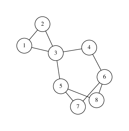
This graph has 6 main eigenvalues, and its characteristic polynomial is

$$\mathop{\phi}\left(\mathbf{A}(G),\lambda\right) =\lambda(\lambda+1)\left(\lambda^{6}-\lambda^{5}-9\lambda^{4}+7\lambda^{3}+19\lambda^{2}-13\lambda\right)\text{.}$$

B.1 Removing a co-duplicate vertex

Consider deleting a co-duplicate vertex (1 or 2) from graph $G$, resulting in a graph $G^{\prime}$. We obtain the characteristic polynomial of $G^{\prime}$ from that of $G$ by first dividing by $\lambda+1$ to remove a $-1$ eigenvalue, then adding $h_{1,2}$ to obtain the necessary displacement in the remaining eigenvalues. So, proceeding as in the earlier examples, using Proposition 2.11 we obtain

$$h_{1,2} =\lambda^{6}+\lambda^{5}-7\lambda^{4}-5\lambda^{3}+9\lambda^{2}-2\lambda\text{.}$$

Using Theorem 2.13 this gives

$$\mathop{\phi}\left(\mathbf{A}(G^{\prime}),\lambda\right) =\lambda\left(\lambda^{6}-8\lambda^{4}+14\lambda^{2}-4\lambda-2\right)\text{.}$$

We can now estimate the shift in the main eigenvalues from $G$ to $G^{\prime}$ using the method of Section 3, after obtaining the necessary functions $f(\lambda)$, $f^{\prime}(\lambda)$, and $f^{\prime\prime}(\lambda)$. Table 4 gives the main eigenvalues of $G$ and $G^{\prime}$, the actual displacement, and the estimates computed using the first-order and second-order approximations of Section 3.

Table 4: Removing a co-duplicate vertex: the eigenvalues of graph $G$ of Figure 1 and $G^{\prime}$ obtained by removing vertex 1 or 2, the actual displacement, and estimates using first- and second-order approximations.

Eigenvalues		Actual	Estimates
$G$	$G^{\prime}$	Displacement	First-order	Second-order
$-2.20$	$-2.18$	$0.0139$	$0.0130$	$0.214,\mathbf{0.0139}$
$-1.89$	$-1.83$	$0.0592$	$0.0642$	$-0.613,\mathbf{0.0581}$
$-1$	—	—	—	—
$0$	$-0.265$	$-0.265$	$0$	-0.5, $\mathbf{0}$
$0$	$0$	$0$	—	—
$0.664$	$0.656$	$-0.00768$	$-0.00763$	$-1.26,\mathbf{-0.00768}$
$1.79$	$1.18$	$-0.609$	$-0.385$	$-17.6,\mathbf{-0.394}$
$2.64$	$2.45$	$-0.192$	$-0.132$	$\mathbf{-0.262}\pm 0.0261j$

B.2 Removing a duplicate vertex

Finally, we delete a duplicate vertex (7 or 8) from graph $G$, resulting in a graph $G^{\prime}$. In this case we obtain the characteristic polynomial of $G^{\prime}$ from that of $G$ by first dividing by $\lambda$ to remove one of the $0$ eigenvalues, then adding $h_{7,8}$ to obtain the necessary displacement in the remaining eigenvalues. So, proceeding as in the earlier examples, using Proposition 2.11 we obtain

$$h_{7,8} =2\lambda^{5}-7\lambda^{3}-4\lambda^{2}+3\lambda+2\text{.}$$

Using Theorem 2.13 this gives

$$\mathop{\phi}\left(\mathbf{A}(G^{\prime}),\lambda\right) =(\lambda+1)\left(\lambda^{6}-\lambda^{5}-7\lambda^{4}+5\lambda^{3}+11\lambda^{2}-7\lambda\right)\text{.}$$

Estimates for the shift in the main eigenvalues from $G$ to $G^{\prime}$ using the first-order and second-order approximations of Section 3 are given in Table 5, together with the main eigenvalues of $G$ and $G^{\prime}$ and the actual displacement.

Table 5: Removing a duplicate vertex: the eigenvalues of graph $G$ of Figure 1 and $G^{\prime}$ obtained by removing vertex 7 or 8, the actual displacement, and estimates using first- and second-order approximations.

Eigenvalues		Actual	Estimates
$G$	$G^{\prime}$	Displacement	First-order	Second-order
$-2.20$	$-1.94$	$0.262$	$0.265$	$\mathbf{0.241}\pm 0.264j$
$-1.89$	$-1.62$	$0.388$	$0.388$	$\mathbf{0.212}\pm 0.346j$
$-1$	$-1$	—	—	—
$0$	—	—	—	—
$0$	$0$	$0$	—	—
$0.664$	$0.618$	$-0.0458$	$-0.0531$	$-0.538,\mathbf{-0.0589}$
$1.79$	$1.46$	$-0.322$	$-0.193$	$-5.01,\mathbf{-0.201}$
$2.64$	$2.47$	$-0.167$	$-0.162$	$\mathbf{-0.263}\pm 0.127j$

References

- [1] E. Heilbronner, Das kompositions-prinzip: Eine anschauliche methode zur elektronen-theoretischen behandlung nicht oder niedrig symmetrischer molekeln im rahmen der mo-theorie, Helvetica Chimica Acta 36 (1) (1953) 170–188.
- [2] E. Heilbronner, Molecular orbitals in homologen reihen mehrkerniger aromatischer kohlenwasserstoffe: I. die eigenwerte von LCAO-MO’s in homologen reihen, Helvetica Chimica Acta 37 (3) (1954) 921–935.
- [3] E. Heilbronner, Ein graphisches verfahren zur faktorisierung der säkulardeterminante aromatischer ringsysteme im rahmen der LCAO–MO-theorie, Helvetica Chimica Acta 37 (3) (1954) 913–921.
- [4] E. Heilbronner, Über einen graphentheoretischen zusammenhang zwischen dem hückel’schen MO-verfahren und dem formalismus der resonanztheorie, Helvetica Chimica Acta 45 (5) (1962) 1722–1725.
- [5] E. Heilbronner, Some comments on cospectral graphs, Math. Chem 5 (1979) 105–133.
- [6] A. J. Schwenk, Computing the characteristic polynomial of a graph, in: Graphs and combinatorics, Springer, 1974, pp. 153–172.
- [7] V. R. Rosenfeld, Another form of the transmission function, Journal of Mathematical Chemistry 51 (10) (2013) 2639–2643.
- [8] M. Thüne, Eigenvalues of matrices and graphs, Ph.D. thesis (1979).
- [9] W. H. Haemers, Interlacing eigenvalues and graphs, Linear Algebra and its applications 226 (1995) 593–616.
- [10] W. H. Haemers, Eigenvalue techniques in design and graph theory, Ph.D. thesis (1980).
-
[11]
L. Lovász, Eigenvalues
of graphs (2007).
URL http://web.cs.elte.hu/~lovasz/eigenvals-x.pdf - [12] M. C. Marino, I. Sciriha, S. K. Simić, D. V. Tošić, More about singular line graphs of trees, Publications de l’Institut Mathématique 79 (93).
- [13] I. Sciriha, M. Debono, M. Borg, P. Fowler, B. Pickup, Interlacing–-extremal graphs, Ars Math. Contemp. 6 (2013) 261–278. doi:10.26493/1855-3974.275.574.
- [14] P. Rowlinson, Co-cliques and star complements in extremal strongly regular graphs, Linear algebra and its applications 421 (1) (2007) 157–162.
- [15] I. Sciriha, S. Farrugia, On the spectrum of threshold graphs, ISRN Discrete Mathematics 2011.
- [16] A. Mohammadian, V. Trevisan, Some spectral properties of cographs, Discrete Mathematics 339 (4) (2016) 1261–1264.
- [17] W. So, Rank one perturbation and its application to the laplacian spectrum of a graph, Linear and Multilinear Algebra 46 (3) (1999) 193–198.
- [18] C.-E. Fröberg, Introduction to numerical analysis, Vol. 6, Addison-Wesley Reading, MA, 1965.
- [19] I. Sciriha, J. A. Briffa, M. Debono, Fast algorithms for indices of nested split graphs approximating real complex networks, Discrete Applied Mathematics 247 (2018) 152–164. doi:10.1016/j.dam.2018.03.054.
- [20] P. Rowlinson, The main eigenvalues of a graph: a survey, Applicable Analysis and Discrete Mathematics (2007) 455–471.
- [21] D. Cvetković, P. Rowlinson, S. Simić, An Introduction to the Theory of Graph Spectra (London Mathematical Society Student Texts), Cambridge: Cambridge University Press, 2001.
- [22] F. Harary, A. Schwenk, The spectral approach to determining the number of walks in a graph, Pacific Journal of Mathematics 80 (2) (1979) 443–449.