Mixing of gravitational wave echoes

Abstract

Gravitational wave (GW) echoes, if they exist, would be a probe to the near-horizon quantum structure of black hole (BH), which has motivated the searching for the echo signals in GW data. We point out that the echo phenomenology related with the potential structure might be not so simple as expected. In particular, if the near-horizon regime of BH is modelled as a multiple-barriers filter, the late-time GW ringdown waveform will exhibit the mixing of echoes, even the superpositions. As a result, the amplitudes of successive echoes might not drop sequentially.

I Introduction

The direct detections of the gravitational wave (GW) signals by the LIGO Scientific and Virgo Collaborations have opened up a new window into the strong gravity regime [1, 2]. The GW signal of binary black holes (BHs) coalescences consists of the inspiral phase, the merger phase and the ringdown phase. It is usually thought that the GW ringdown signal is a powerful hint of the existence of BH horizon. However, Cardoso et al. have pointed out that the ringdown waveform detected is related only with the light ring of the post-merger object rather than the horizon [3], see [4] for a review. Thus although the GW events observed are compatible with the BHs predicted in General Relativity (GR) [5, 6], it is still possible that the new physics might present near the horizon [7, 8].

It is well-known that the BH based on GR suffered from the information paradox, which has inspired the modification to GR BH, e.g.“firewalls”[9, 10],“fuzzy ball”[11]. Usually, in such modifications, as well as in the alternatives to GR BH, e.g. gravastar[12, 13] (see also its origin in early universe [14]), boson star[15, 16, 17], the Schwarzschild horizon may be replaced by a reflective surface or barrier. It has been showed that if such a surface reflects GW, the ringdown waveform of post-merger object is initially almost similar to the ringdown signal of BH, but at late-time will show itself a series of “echoes” [3, 18, 19, 20]. see also [21, 22, 23, 24, 25, 26, 27, 28, 29, 30] for relevant explorations.

It has been widely thought that if they exist, the echoes would be the probes of quantum gravity physics at the near-horizon regime, which has motivated the searching for the echo signals in GW data [20, 31, 32, 33], see also recent progress [34, 35, 36, 37]. It has been showed in Refs.[26] that if the post-merger compact object is unstable, which is collapsing into a BH, in the post-merger ringdown waveform the echo intervals will inevitably increase with the time, see also [38]. Relevant studies enriched the echo phenomenology and helped to the searching for the echo signals [37].

Actually, the echo waveforms related with the potential physics near the horizon might be far complicated than expected. In a pioneer work, Bekenstein and Mukhanov [39, 40] have pointed out that the area of BH horizon might be quantized $A\sim(integer)l_{P}^{2}$ ($l_{P}^{2}$ is the Planck area). As a result, the wavelength of GWs absorbed or emitted by a BH is also quantized, see also [41]. Recently, in Ref.[42], Cardoso, Foit and Kleban have modelled the near-horizon regime of such BHs as a filter consisting of a couple of reflective barriers, which just absorbs the GW with some frequencies and reflects the rest, and found that in the post-merger ringdown waveform the echo signal will be distorted.

Inspired by Ref.[42], we will investigate the echo phenomenology of the BH with a multiple-barriers filter at its near-horizon regime in details. In Sec.II, we model our BH setup, and numerically show the ringdown waveforms of such post-merger BH. Besides the echo signal is distorted, we observe that the mixing and superpositions of echoes also present. As a result, the amplitudes of successive echoes might not drop sequentially. In Sec.III, with the Dyson series method proposed by Correia and Cardoso [27], we analyse the corresponding ringdown waveforms. And we conclude in Sec.IV

II The setup

II.1 Near-horizon (multiple) barriers

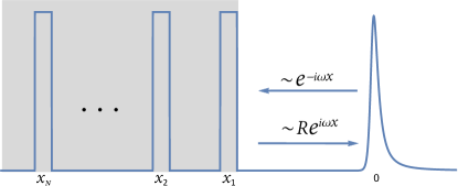
Figure 1: The near-horizon structure of BH in the setup of Sec.II. In the tortoise coordinate, the right-most barrier is $V^{BH}(x)$ in (3), while the effective potential $V_{eff}(x)$ in (3) corresponds to a set of barriers in the shadow region.

Inspired by Ref.[42], we model the (nonspining for simplicity) BH as such an object, which obeys the Schwarzschild metric

$$ds^{2}=-Bdt^{2}+{dr^{2}\over B}+r^{2}d\Omega^{2},\quad\left(B=1-{2M\over r}\right)$$ (1)

at its radius $r>r_{1}$, but at its near-horizon regime $(2M<r<r_{1})$, where ${r_{1}\over 2M}-1\ll 1$, the quantum effect of BH would bring the distinct structure, see Fig.1 plotted in the tortoise coordinate $x=r+2M\log({r\over 2M}-1)$.

In the tortoise coordinate, the Regge-Wheeler equation for the axial gravitational perturbation is

$$\left[-\frac{\partial^{2}}{\partial t^{2}}+\frac{\partial^{2}}{\partial x^{2}}-V(x)\right]\Psi(t,x)=0,$$ (2)

with

$$V(x)=V_{l}^{BH}(r(x))+V_{eff}(r(x)),$$ (3)

where $V_{l}^{BH}(r(x))$ is the barrier $V_{l}^{BH}(r)=B\left[\frac{l(l+1)}{r^{2}}+\frac{(1-s^{2})B^{\prime}}{r}\right]$ but written in the tortoise coordinate $x$, $l\geqslant s$ is the multipolar index and $s=2$ [43]. We refer $V_{l}^{BH}(x)$ as the potential barrier at the photon sphere, which is equivalent to that of GR BH. We have put the unknown physics at the near-horizon regime of BH into $V_{eff}(x)$, which is either a single reflective surface, or a complicated barrier, or a set of multiple barriers (equivalently, a special boundary condition).

The ringdown burst incident towards the horizon will be reflected repeatedly between the barrier $V_{eff}(x)$ and $V_{l}^{BH}(x)$. Thus as has been pointed out in Refs.[3, 18] that the ringdown waveform of post-merger BH will consist of the primary signal, almost similar to that of GR BH, and a series of echoes. Generally, $V_{eff}(x)$ related with the potential physics might be not a simple reflective surface, but a set of multiple barriers, as argued in Ref.[42]. Relevant echo phenomenology has not yet been explored completely.

II.2 Waveforms of echoes

As an illustration, we will focus on the case with $l=2$. Using the Laplace transform $\tilde{\Psi}(\omega,x)=\int_{0}^{\infty}\Psi(t,x)e^{i\omega t}dt$ [19], one rewrite Eq.(2) as

$$\left[\frac{\partial^{2}}{\partial x^{2}}+\omega^{2}-V(x)\right]\tilde{\Psi}(\omega,x)={\cal I},$$ (4)

with ${\cal I}(\omega,x)=i\omega\Psi(0,x)-{\dot{\Psi}}(0,x)$, where $\Psi(0,x)$ and ${\dot{\Psi}}(0,x)$ are the initial conditions of $\Psi(t,x)$. We consider $V_{eff}(x)$ in (3) as

$$V_{eff}(x)=2\sum_{j=1}^{N}V_{j}\delta(x-x_{j}),$$ (5)

where $2V_{j}$ is the height of Delta barrier at $x_{j}$, which is a simplified model of multiple barriers, but is sufficient to catch the echo phenomenology of the setup depicted in Fig.1. Solving out $\tilde{\Psi}(\omega,x)$, we may get $\Psi(t,x)$ by

$$\Psi(t,x)={1\over 2\pi}\int_{-\infty}^{\infty}\tilde{\Psi}(\omega,x)e^{-i\omega t}d\omega.$$ (6)

We set

$$\Psi(0,x)=e^{-(x-5)^{2}/9},\quad\,{\partial_{t}\Psi}(0,x)=0,$$ (7)

($2M=1$ for convenience) and also $N=2$ in (5), i.e. $V_{eff}(x)=2\sum_{j=1}^{2}V_{j}\delta(x-x_{j})$ consists of a couple of Delta barriers, and plot the corresponding ringdown waveforms $\Psi(t,x)$ in Figs.2, 3, 4 and 5 for different values of $x_{1}$ and $x_{2}$, respectively, where the height of barriers are $2V_{1}=0.5$ or $1$, $2V_{2}=60$.

We see in Fig.2 that after the primary ringdown burst a series of echoes present, as expected, but the intervals of successive echoes seems not to equal. Here, the case is different from that in Ref.[26], where the change of echo intervals is caused by the shift of reflective surface or barrier. In addition, as showed in Ref.[42], when $x_{2}$ is very close to $x_{1}$, so that $2|x_{2}-x_{1}|\lesssim\Delta_{echo}$, where $\Delta_{echo}$ is the width of echo waveform, the echoes will be significantly distorted, see Fig.3.

We see in Fig.4 that for $|x_{2}-x_{1}|=|x_{1}|$, the echoes reflected by $V_{eff}(x)$ will present at $t_{n}-t_{ringdown}=2n|x_{1}|$, but the echoes exhibit certain superposition and cancellation, which occur at $t_{n}-t_{ringdown}=2n|x_{1}|$ ($n\geqslant 2$), so that the amplitudes of successive echoes seem be out of order. The amplitude of echo after the superposition will be amplified. Actually, even if $|x_{2}-x_{1}|=|x_{1}|$, in the physical coordinate $r$ the barrier $V_{1}$ is far closer to $V_{2}$ than the barrier $V^{BH}(r)$. Similarly, in Fig.5, we set $|x_{2}-x_{1}|=3|x_{1}|$, and see that the superposition and cancellation occur at $t_{n}-t_{ringdown}=2n|x_{1}|$ ($n\geqslant 4$).

We also plot the ringdown waveforms for $V_{eff}(x)$ with $N=3$ in Appendix A. The waveforms are qualitatively similar to the cases with $N=2$.

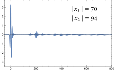
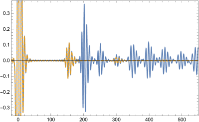
Figure 2: Ringdown waveforms with respect to $t$. The right panel is the magnification of the left panel. As a comparison, the yellow curve in the right panel is the ringdown waveform with a single Delta barrier near the horizon ($|x_{1}|=70$).

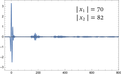
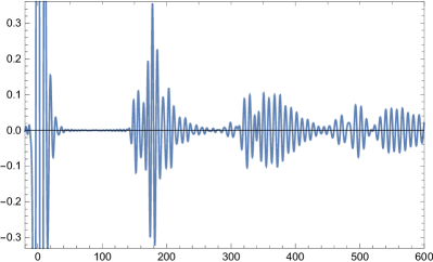
Figure 3: Ringdown waveforms with respect to $t$. The right panel is the magnification of the left panel.

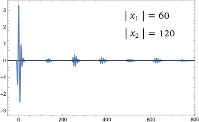
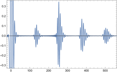
Figure 4: Ringdown waveforms with respect to $t$ in the model with $|x_{2}-x_{1}|=|x_{1}|$. The right panel is the magnification of the left panel.

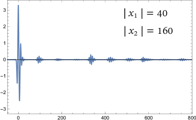
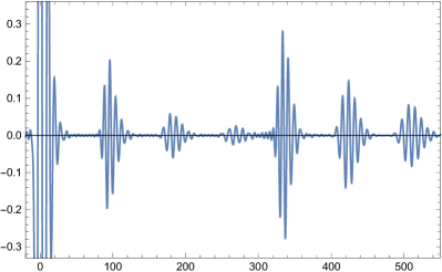
Figure 5: Ringdown waveforms with respect to $t$ in the model with $|x_{2}-x_{1}|=3|x_{1}|$. The right panel is the magnification of the left panel.

III Analytic studies

III.1 Boundary conditions

It is interesting to have an insight into the echo phenomenology showed in Sect.II.1 by analytically solving Eq.(4). We first set the boundary conditions.

The wave $\tilde{\Psi}$ should obey the outgoing wave condition

$$\tilde{\Psi}\sim e^{i\omega x}$$ (8)

as $x\rightarrow\infty$. As imagined in Sect.II, the physics of GR BH has been modified at $r<r_{1}$ (equivalently $x<x_{1}$ in the tortoise coordinate). However, in despite of what the potential barrier $V_{eff}(x)$ looks like, one always may regard the surface at $x_{1}$ as an effective boundary, near which $\tilde{\Psi}$ should satisfy [23]

$$\tilde{\Psi}\sim e^{-i\omega x}+R_{eff}(\omega)e^{i\omega x},$$ (9)

where $R_{eff}(\omega)$ is the effective reflection coefficient (RC). In particular, one has $R_{eff}(\omega)=0$ for the GR BH (without the barrier $V_{eff}(x)$), and $R_{eff}(\omega)=-e^{2i\omega|x_{1}|}$ for the boundary condition ${\tilde{\Psi}}(\omega,x_{1})=0$ at $x_{1}$. Thus in certain sense, $R_{eff}(\omega)$ actually encodes the internal structure of $V_{eff}(x)$.

Considering that $V_{eff}(x)=2\sum_{j=1}^{2}V_{j}\delta(x-x_{j})$ consists of a couple of barriers, we have

$$R_{2,eff}=R_{1}+R_{2}T_{1}^{2}\sum_{m=0}^{\infty}(\tilde{R}_{1}R_{2})^{m}=R_{1}+\frac{R_{2}T_{1}^{2}}{1-\tilde{R}_{1}R_{2}},$$ (10)

where the integer $m$ corresponds to the roundtrip number of GW between the barriers $V_{1}$ and $V_{2}$. Here, for the Delta barrier with the height $2V_{j}(j=1,2\cdots)$,

$$R_{j}=-\frac{V_{j}}{V_{j}-i\omega}e^{-2i\omega x_{j}},\quad\tilde{R}_{j}=-\frac{V_{j}}{V_{j}-i\omega}e^{2i\omega x_{j}},\quad T_{j}=-\frac{i\omega}{V_{j}-i\omega}.$$ (11)

$R_{j}$ is the RC of a single barrier $V_{j}$ for the wave incident from right, while $\tilde{R}_{j}$ is that from left, $T_{j}$ is the TC of a single barrier $V_{j}$. Thus we have

$${\tilde{R}}_{1}R_{2}=\left(\frac{V_{1}}{V_{1}-i\omega}\right)\left(\frac{V_{2}}{V_{2}-i\omega}\right)e^{2i\omega(x_{1}-x_{2})}.$$ (12)

Considering that $V_{eff}(x)=2\sum_{j=1}^{3}V_{j}\delta(x-x_{j})$, i.e.3-Delta barrier, we have the effective RC ${R}_{3,eff}$ as

$${R}_{3,eff}={R}_{2,eff}+\frac{R_{3}{T}_{2,eff}}{1-\tilde{R}_{2,eff}R_{3}},$$ (13)

where $R_{2,eff}$ is the effective RC (10) of 2-Delta barriers, $\tilde{R}_{2,eff}$ is that for the wave incident from left, and $R_{3}$ is the RC of a single Delta barrier at $x_{3}$, see (11), $T_{2,eff}$ is the effective TC, see Appendix B for the expressions of $\tilde{R}_{2,eff}$ and $T_{2,eff}$. In Appendix B, we also verified Eqs.(10) and (13).

The system with 3-Delta barriers actually corresponds to that with 2-barrier (the barriers $V_{3}$ and $V_{2,eff}$). Thus with the replacements $R_{1}\rightarrow R_{2,eff}$, $T_{1}\rightarrow T_{2,eff}$ and $R_{2}\rightarrow R_{3}$ in Eq.(10), we will immediately get Eq.(13). It is not difficult to straightly write out the effective RC of $j$-Delta barriers

$${R}_{j,eff}={R}_{(j-1),eff}+\frac{R_{j}{T}_{(j-1),eff}^{2}}{1-\tilde{R}_{(j-1),eff}R_{j}}.$$ (14)

Thus with (11) and the recursive relationship (14), the full result of the effective RC ${R}_{N,eff}$ of $N$-Delta barriers may be worked out.

Physically, Eq.(4) is equivalent to

$$\left[\frac{\partial^{2}}{\partial x^{2}}+\omega^{2}-V^{BH}(x)\right]\tilde{\Psi}(\omega,x)={\cal I},$$ (15)

with the boundary condition (8) and (9), where $V_{eff}(x)$ (related with the near-horizon physics of BH) in (3) has been encoded in $R_{eff}(\omega)$.

III.2 Review on the Dyson series method

To analyse the ringdown waveforms, we will apply the Dyson series method proposed in Ref.[27]. Here, we briefly review it.

Defining the operator ${\cal A}=\frac{\partial^{2}}{\partial x^{2}}+\omega^{2}$, we have ${\cal A}^{-1}\tilde{\Psi}=\int g(x,x^{\prime})\tilde{\Psi}dx^{\prime}$, where Green’s function $g(x,x^{\prime})$ satisfying the boundary conditions (8) and (9) is

$$g(x,x^{\prime})=\frac{e^{i\omega|x-x^{\prime}|}+R_{eff}e^{i\omega(x+x^{\prime})}}{2i\omega}.$$ (16)

Here, $R_{eff}$ is the effective RC of $V_{eff}(x)$, and for a couple of Delta barriers, $R_{eff}$ equals to $R_{2,eff}$ in Eq.(10). According to (16), $g(x,x^{\prime})$ may be separated into $g=g_{O}+{R}_{eff}g_{R,eff}$ with

$$g_{O}(x,x^{\prime})=\frac{e^{i\omega|x-x^{\prime}|}}{2i\omega},\quad g_{{R,eff}}(x,x^{\prime})=\frac{e^{i\omega(x+x^{\prime})}}{2i\omega},$$ (17)

which correspond to that of open system without $V_{eff}(x)$ and that reflected by $V_{eff}(x)$, respectively. As a result, we have ${\cal A}^{-1}={\cal A}^{-1}_{O}+{\cal A}^{-1}_{R,eff}$ with

$${\cal A}^{-1}_{O}\tilde{\Psi}=\int g_{O}(x,x^{\prime})\tilde{\Psi}dx^{\prime},\quad{\cal A}^{-1}_{R,eff}\tilde{\Psi}=R_{eff}\int g_{R,eff}(x,x^{\prime})\tilde{\Psi}dx^{\prime},$$ (18)

We rewrite Eq.(15) as $\tilde{\Psi}={\cal A}^{-1}{\cal I}+{\cal A}^{-1}\hat{V}^{BH}\tilde{\Psi}$, which is

$$\tilde{\Psi} = \left({\cal A}^{-1}_{O}+{\cal A}^{-1}_{R,eff}\right){\cal I}+\left({\cal A}^{-1}_{O}+{\cal A}^{-1}_{R,eff}\right)\hat{V}^{BH}\tilde{\Psi}.$$ (19)

The Dyson series solution of Eq.(19) is

$$\tilde{\Psi}=\tilde{\Psi}_{O}+\sum_{n=1}^{\infty}\tilde{\Psi}_{n}$$ (20)

with

$$\tilde{\Psi}_{O}=\sum_{p=0}^{\infty}\left({\cal A}_{O}^{-1}\hat{V}^{BH}\right)^{p}\left({\cal A}_{O}^{-1}{\cal I}\right),$$ (21)

$$\tilde{\Psi}_{n}=\sum_{p=n}^{\infty}\sum_{\{p,n\}}\left({\cal A}_{O}^{-1}\right)^{p-n}\left({\cal A}^{-1}_{R,eff}\right)^{n}\left(\hat{V}^{BH}\right)^{p-1}{\cal I},$$ (22)

where the sum $\sum_{\{p,n\}}$ only includes all distinct possibilities of ordering $n$ ${\cal A}^{-1}_{R,eff}$ in $p$ spots.

We actually have the infinite number of Dyson series with the barrier $V^{BH}$ at the photon sphere. Here, $\tilde{\Psi}_{O}$ is the waveform of open system without the effective barrier $V_{eff}$, which is irrelevant with ${\cal A}_{R,eff}^{-1}$, while the “reflected” waveform $\tilde{\Psi}_{n}\sim({\cal A}^{-1}_{R,eff})^{n}\sim R_{eff}^{n}$, where $n$ is the roundtrips number of wave between the barriers $V_{eff}(x)$ and $V^{BH}(x)$. The formal solution (22) is actually equivalent to

$$\tilde{\Psi}_{n}(\omega,x) = {R}^{n}_{eff}\sum_{p=n}^{\infty}\int\sum_{\{p,n\}}g_{R,eff}(x,x^{\prime}_{1})\cdots g_{R,eff}(x^{\prime}_{n-1},x^{\prime}_{n})$$ (23)

$$g_{O}(x^{\prime}_{n},x^{\prime}_{n+1})\cdots g_{O}(x^{\prime}_{p-1},x^{\prime}_{p})V^{BH}(x^{\prime}_{1})\cdots V^{BH}(x^{\prime}_{p-1}){\cal I}(\omega,x^{\prime}_{p})dx^{\prime}_{1}\cdots dx^{\prime}_{p},$$

which is a multiple integrals.

We will only be interested in the waveform $\tilde{\Psi}_{n}$. The GR barrier $V^{BH}$ at the photon sphere must be speculated to calculate $\tilde{\Psi}_{n}$. However, it is not required for our analysis. Here, we assumed $V^{BH}=2V_{0}\delta(x)$ for simplicity (but without loss of physics we care). Now, the multiple integrals in (23) may be reduced to one integral only for $x_{p}^{\prime}=x^{\prime}$. The corresponding $\tilde{\Psi}_{n}$ has been calculated in Ref.[27],

$$\tilde{\Psi}_{n}(\omega,x)={R}^{n}_{eff}\int dx^{\prime}{\cal I}(\omega,x^{\prime})\left[R_{0}^{n-1}{e^{i\omega(x+x^{\prime})}\over{2i\omega}}+R_{0}^{n+1}{e^{i\omega(|x|+|x^{\prime}|)}\over{2i\omega}}+R_{0}^{n}{e^{i\omega(x+|x^{\prime}|)}+e^{i\omega(x^{\prime}+|x|)}\over{2i\omega}}\right],$$ (24)

where

$$R_{0}(\omega)=-\frac{V_{0}}{V_{0}-i\omega}$$ (25)

is the RC of a single Delta barrier at $x_{0}=0$, see (11).

III.3 Mixing of echoes

We will analyse the mixing of echoes with $N=2$ in (5), i.e. 2-Delta barriers, as example. The cases with $N\geqslant 3$ are similar.

According to Eq.(24), the late-time ringdown waveform is closely related with ${R}^{n}_{eff}$. With (11), we rewrite $R_{eff}$ in Eq.(10) as

$${R}_{eff}=R_{1}\left[1+\left(\frac{i\omega}{V_{1}}\right)^{2}\sum_{m=1}^{\infty}({\tilde{R}}_{1}R_{2})^{m}\right].$$ (26)

We have

$$R_{eff}^{n}= R_{1}^{n}\sum_{k=0}^{n}\left(\begin{array}[]{ccc}n\\ k\end{array}\right)\left(\frac{i\omega}{V_{1}}\right)^{2k}\left[\sum_{m=1}^{\infty}({\tilde{R}}_{1}R_{2})^{m}\right]^{k}$$ (29)

$$= R_{1}^{n}\sum_{k=0}^{n}\left(\begin{array}[]{ccc}n\\ k\end{array}\right)\left(\frac{i\omega}{V_{1}}\right)^{2k}\sum_{k_{m}\geq 0,\sum_{m}k_{m}=k}\frac{k!}{k_{1}!k_{2}!\cdots k_{m}!\cdots}\prod_{m=1}^{\infty}\left[({\tilde{R}}_{1}R_{2})^{m}\right]^{k_{m}}.$$ (32)

We explain it as follows. When $k=0$, all $k_{m}$ must satisfy $k_{m}=0$, so $R_{eff}^{n}=R_{1}^{n}$. When $k=1$, all $k_{m\neq m^{\prime}}=0$ except for $k_{m^{\prime}}=1$ ($m^{\prime}$ runs from $1$ to $\infty$), we have

$$R_{eff}^{n}\sim R_{1}^{n}\sum_{k_{m}\geq 0,\sum_{m}k_{m}=k}\prod_{m=1}^{\infty}\left[({\tilde{R}}_{1}R_{2})^{m}\right]^{k_{m}}=R_{1}^{n}\sum_{m=1}^{\infty}({\tilde{R}}_{1}R_{2})^{m}.$$ (33)

Similarly, when $k=2$, either all $k_{m\neq m^{\prime},m^{\prime\prime}}=0$ except for $k_{m^{\prime}}=1$, $k_{m^{\prime\prime}}=1$ ($m^{\prime}\neq m^{\prime\prime}$), or all $k_{m\neq m^{\prime}}=0$ except for $k_{m^{\prime}}=2$.

Combining (32) and the solution (24) of ${\tilde{\Psi}}_{n}$, we have the ${\tilde{n}}$th echo (in the frequency-domain) of the ringdown burst as

$$\tilde{\Psi}_{\tilde{n}}(\omega,x) \sim R_{1}^{n}\prod_{m=1}^{\infty}\left[({\tilde{R}}_{1}R_{2})^{m}\right]^{k_{m}}e^{i\omega x}$$ (34)

$$= e^{i\omega x}\exp{\left[-2i\omega nx_{1}-2i\omega(x_{2}-x_{1}){\sum_{m=1}^{\infty}mk_{m}}\right]}$$

for $\sum_{m}k_{m}=k\leqslant n$, where ${\tilde{R}}_{1}R_{2}$ is showed in (12). We eventually get ${\tilde{\Psi}}_{\tilde{n}}(t,x)$ through $\Psi_{\tilde{n}}(t,x)\sim\int\tilde{\Psi}_{\tilde{n}}(\omega,x)e^{-i\omega t}d\omega$. According to Eq.(34), it is found that after the primary ringdown signal at $t_{ringdown}$, the $\tilde{n}$th echo will appear at

$$t_{\tilde{n}}-t_{ringdown}=2\left[n|x_{1}|+|x_{1}-x_{2}|{\sum_{m=1,\sum_{m}k_{m}=k\leqslant n}^{\infty}mk_{m}}\right].$$ (35)

When $m=0$, we have $t_{\tilde{n}}-t_{ringdown}=2n|x_{1}|$, the ordinal number ${\tilde{n}}=1,2,3\cdots$ of echoes coincides with $n$, which is just the well-known result [3] in single barrier model. The case with the multiple barriers is different. We see that for a fixed $n$, a series of “echoes” (so-called the sub-echo) of the $n$th echo will also present with the intervals

$$\Delta t_{k,k_{m}}=2|x_{1}-x_{2}|{\sum_{m=1,\sum_{m}k_{m}=k\leqslant n}^{\infty}mk_{m}}$$ (36)

after the $n$th echo. Thus the ordinal number ${\tilde{n}}=1,2,3\cdots$ of echoes will be arranged by not only $n$, but $k$, $m$, $x_{1}$ and $x_{2}$. This suggests that the echoes are mixing.

The first (${\tilde{n}}=1$) echo presents at $t_{1}-t_{ringdown}=2|x_{1}|$, which corresponds to $k=0$ (all $k_{m}=0$) for $n=1$ in Eq.(35). When $|x_{1}-x_{2}|<|x_{1}|$, the second (${\tilde{n}}=2$) echo will present at $t_{2}-t_{ringdown}=2|x_{1}|+2|x_{1}-x_{2}|$, which corresponds to $k=1$ (all $k_{m}=0$ except for $k_{1}=1$) for $n=1$ and actually is the sub-echo of the $(n=1)$th echo. Its second sub-echo is at $t-t_{ringdown}=2|x_{1}|+4|x_{1}-x_{2}|$, which also corresponds to $k=1$ but all $k_{m}=0$ except for $k_{2}=1$, see Fig.2 in Sect.IIB. Moreover, if $|x_{1}-x_{2}|\ll|x_{1}|$, we will have $t_{2}-t_{ringdown}\simeq t_{1}-t_{ringdown}$ (the barrier $V_{2}$ is very close to $V_{1}$, so that $2|x_{2}-x_{1}|\lesssim\Delta_{echo}$), the first echo will be significantly affected by its sub-echo, and distorted, as found in Ref.[42], see also Fig.3 in Sect.IIB.

Generally, it is hardly possible that the amplitude ($\sim|R_{1}|^{2}$) of echo with $n=2$ is larger than that ($\sim|R_{1}|$) with $n=1$, since $|R_{1}|\leqslant 1$. Thus in the single barrier model, the amplitudes of successive echoes drop sequentially. However, when the multiple barriers are considered, the case is altered. It is possible that the amplitude ${\cal A}_{{\tilde{n}}=2}\sim|R_{2}T_{1}^{2}|$ of the second echo is larger than ${\cal A}_{{\tilde{n}}=1}\sim|R_{1}|$. We plot ${\cal A}_{{\tilde{n}}=2}$ and ${\cal A}_{{\tilde{n}}=1}$ with respect to $\omega$ in Fig.6, respectively, and see that ${\cal A}_{{\tilde{n}}=2}>{\cal A}_{{\tilde{n}}=1}$ is possible, if $V_{2}>V_{1}$.

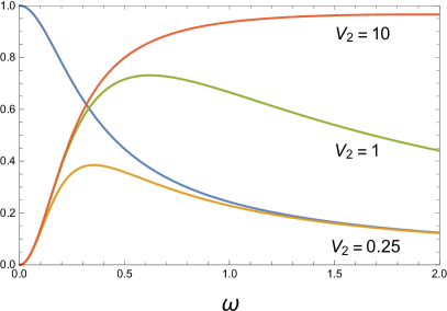
Figure 6: The blue curve is the amplitude ${\cal A}_{{\tilde{n}}=1}$ of the first echo with $V_{1}=0.25$, and the others are ${\cal A}_{{\tilde{n}}=2}$ with $V_{1}=0.25$, $V_{2}=0.25,1,10$, respectively.

Another possibility causing the anomalies of echo amplitudes is that if

$$n|x_{1}|+|x_{1}-x_{2}|{\sum_{m=1,\sum_{m}k_{m}=k\leqslant n}^{\infty}mk_{m}}=n^{\prime}|x_{1}|+|x_{1}-x_{2}|{\sum_{m^{\prime}=1,\sum_{m^{\prime}}k^{\prime}_{m^{\prime}}=k^{\prime}\leqslant n^{\prime}}^{\infty}m^{\prime}k^{\prime}_{m^{\prime}}},$$ (37)

the echoes with different $n$ will superpose each other. The superposition of echoes is the unique phenomenon happening only in the multiple barriers models.

In Fig.4 of Sect.IIB, where $|x_{1}|=|x_{1}-x_{2}|$, we see that the second echo presents at $t_{2}-t_{ringdown}=4|x_{1}|$, which is just the superposition of the $(n=2)$th echo with the sub-echo ($n^{\prime}=1,k^{\prime}=1,$ all $k^{\prime}_{m^{\prime}}=0$ except for $k^{\prime}_{1}=1)$ of the $(n=1)$th echo. And so on, the third echo presents at $t_{3}-t_{ringdown}=6|x_{1}|$, which is the superposition of the $(n=3)$th echo with the sub-echo $(n^{\prime}=2,k^{\prime}=1$, all $k^{\prime}_{m^{\prime}}=0$ except for $k^{\prime}_{1}=1)$ and the sub-echo $(n^{\prime\prime}=1,k^{\prime\prime}=1,$ all $k^{\prime\prime}_{m^{\prime\prime}}=0$ except for $k^{\prime\prime}_{2}=1)$.

IV Discussion

Quantum gravity physics, invoked by the information paradox of BH, might result in some microstructure at the near-horizon regime of BH, which may reflect GWs. The GW echoes, if they exist, will be a promising probe of such physics, which has excited the searching for the echo signals in GW data.

However, the potential physics responsible for the GW echoes is actually unknown, which is still in the exploration, so the echo phenomenology might be not so simple as expected. Inspired by Ref.[42], we show that if the near-horizon regime of BH is modelled as a multiple-barriers filter with different spacings between barriers, the GW ringdown waveform of post-merger BH will exhibit the mixing of echoes, even the superpositions. As a result, the echo amplitudes might not drop sequentially.

Though the post-merger BH we considered is a nonspinning BH, extending it to the Kerr BH is straight. The effect of ergoregion in Kerr BH on the GW echoes has been studied in Refs.[44, 45]. In addition, it is interesting to present a full “template” of the ringdown waveforms with the mixing and superpositions of echoes, along the line in Refs.[29]. It is also interesting to check what a stochastic GW background such echoes will result in, which might be also substantially detectable [46].

It is actually possible to find the GW echoes, as more and more GW events with higher signal-to-noise ratio are detected [4]. Our work suggests that the echo phenomenology related with the potential physics might be far richer than expected, so identifying relevant signals will be a more challenging task.

Acknowledgments

We would like to thank the cooperation with Jun Zhang and Shuang-Yong Zhou at the initial stage of this project, and also thank Yu-Tong Wang for discussion. This work is supported by NSFC, Nos.11575188,11690021.

Appendix A The echo waveforms for $N=3$

We plot the echo waveforms for $V_{eff}(x)$ with $N=3$ in this Appendix.

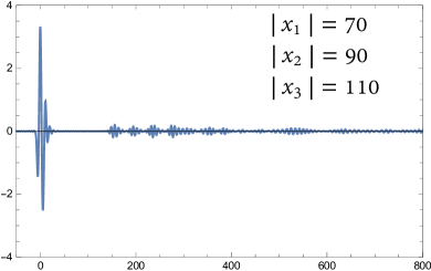
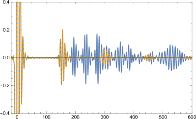
Figure 7: Ringdown waveforms with respect to $t$. The right panel is the magnification of the left panel. As a comparison, the yellow curve in the right panel is the ringdown waveform with a single Delta barrier near the horizon ($|x_{1}|=70$).

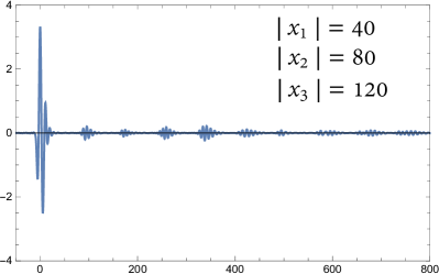
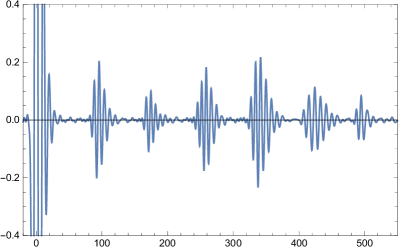
Figure 8: Ringdown waveforms with respect to $t$ in the model with $|x_{3}-x_{1}|=|x_{2}-x_{1}|=|x_{1}|$. The right panel is the magnification of the left panel.

Appendix B The effective RC for $N=2,3$

In this Appendix, we will briefly verify Eqs.(10) and (13).

We consider $N=2$ first. The Delta barriers at $x_{1}$ and $x_{2}$ divide the $x$-space into the regions I, II, III. The waves ${\tilde{\Psi}}_{I}=e^{-i\omega x}+A_{1}e^{i\omega x}$, ${\tilde{\Psi}}_{II}=A_{2}e^{-i\omega x}+A_{3}e^{i\omega x}$ and ${\tilde{\Psi}}_{III}=A_{4}e^{-i\omega x}$ in corresponding regions must satisfy

$$e^{-i\omega x_{1}}+A_{1}e^{i\omega x_{1}}=A_{2}e^{-i\omega x_{1}}+A_{3}e^{i\omega x_{1}},$$ (38)

$$A_{2}e^{-i\omega x_{2}}+A_{3}e^{i\omega x_{2}}=A_{4}e^{-i\omega x_{2}},$$ (39)

$$-i\omega e^{-i\omega x_{1}}+i\omega A_{1}e^{i\omega x_{1}}+i\omega A_{2}e^{-i\omega x_{1}}-i\omega A_{3}e^{i\omega x_{1}}=2V_{1}\left(e^{-i\omega x_{1}}+A_{1}e^{i\omega x_{1}}\right),$$ (40)

$$-i\omega A_{2}e^{-i\omega x_{2}}+i\omega A_{3}e^{i\omega x_{2}}+i\omega A_{4}e^{-i\omega x_{2}}=2V_{2}A_{4}e^{-i\omega x_{2}},$$ (41)

at $x_{1}$ and $x_{2}$. The effective RC is

$$R_{2,eff}=A_{1}=\frac{V_{2}(V_{1}+i\omega)e^{-2i\omega x_{2}}-V_{1}(V_{2}-i\omega)e^{-2i\omega x_{1}}}{(V_{1}-i\omega)(V_{2}-i\omega)-V_{1}V_{2}e^{2i\omega(x_{1}-x_{2})}},$$ (42)

$${\tilde{R}}_{2,eff}=\frac{V_{1}(V_{2}+i\omega)e^{2i\omega x_{1}}-V_{2}(V_{1}-i\omega)e^{2i\omega x_{2}}}{(V_{1}-i\omega)(V_{2}-i\omega)-V_{1}V_{2}e^{2i\omega(x_{1}-x_{2})}},$$ (43)

while the effective TC is

$$T_{2,eff}=A_{4}=\frac{-\omega^{2}}{(V_{1}-i\omega)(V_{2}-i\omega)-V_{1}V_{2}e^{2i\omega(x_{1}-x_{2})}}.$$ (44)

Thus with (11), we straightly have

$$R_{1}+\frac{R_{2}T_{1}^{2}}{1-\tilde{R}_{1}R_{2}}$$

$$=-\frac{V_{1}}{V_{1}-i\omega}e^{-2i\omega x_{1}}+\frac{-\frac{V_{2}}{V_{2}-i\omega}\left(\frac{-i\omega}{V_{1}-i\omega}\right)^{2}e^{-2i\omega x_{2}}}{1-\left(\frac{V_{1}}{V_{1}-i\omega}\right)\left(\frac{V_{2}}{V_{2}-i\omega}\right)e^{2i\omega(x_{1}-x_{2})}}$$

$$=\left(-\frac{1}{V_{1}-i\omega}\right)\left[V_{1}e^{-2i\omega x_{1}}+\frac{V_{2}(-i\omega)^{2}e^{-2i\omega x_{2}}}{(V_{1}-i\omega)(V_{2}-i\omega)-V_{1}V_{2}e^{2i\omega(x_{1}-x_{2})}}\right]$$

$$={R}_{2,eff},$$ (45)

Figure 9: $|{R}_{2,eff}|^{2}$ and $|{T}_{2,eff}|^{2}$ with parameters $V_{1}=V_{2}=0.5$, $x_{1}=-10$ and $x_{2}=-20$ .

Similarly, the effective RC for $N=3$ is

$${R}_{3,eff}=\frac{P}{Q}$$ (46)

where

$$P =-V_{1}(V_{2}-i\omega)(V_{3}-i\omega)e^{-2i\omega x_{1}}$$

$$+V_{2}(V_{1}-i\omega)(V_{3}-i\omega)e^{-2i\omega x_{2}}-V_{3}(V_{1}+i\omega)(V_{2}+i\omega)e^{-2i\omega x_{3}}+V_{1}V_{2}V_{3}e^{2i\omega(x_{2}-x_{1}-x_{3})},$$ (47)

$$Q =(V_{1}-i\omega)(V_{2}-i\omega)(V_{3}-i\omega)$$

$$-V_{1}V_{2}(V_{3}-i\omega)e^{2i\omega(x_{1}-x_{2})}+V_{1}V_{3}(V_{2}+i\omega)e^{2i\omega(x_{1}-x_{3})}-V_{2}V_{3}(V_{1}-i\omega)e^{2i\omega(x_{2}-x_{3})}.$$ (48)

Considering (42), (43) and (44), we have

$${R}_{2,eff}+\frac{R_{3}{T}_{2,eff}^{2}}{1-\tilde{R}_{2,eff}R_{3}}$$

$$=\frac{V_{2}(V_{1}+i\omega)e^{-2i\omega x_{2}}-V_{1}(V_{2}-i\omega)e^{-2i\omega x_{1}}}{(V_{1}-i\omega)(V_{2}-i\omega)-V_{1}V_{2}e^{2i\omega(x_{1}-x_{2})}}+\frac{\left(-\frac{V_{3}}{V_{3}-i\omega}e^{-2i\omega x_{3}}\right)\left[\frac{-\omega^{2}}{(V_{1}-i\omega)(V_{2}-i\omega)-V_{1}V_{2}e^{2i\omega(x_{1}-x_{2})}}\right]^{2}}{1-\frac{V_{1}(V_{2}+i\omega)e^{2i\omega x_{1}}-V_{2}(V_{1}-i\omega)e^{2i\omega x_{2}}}{(V_{1}-i\omega)(V_{2}-i\omega)-V_{1}V_{2}e^{2i\omega(x_{1}-x_{2})}}\left(-\frac{V_{3}}{V_{3}-i\omega}e^{-2i\omega x_{1}}\right)}$$

$$=\frac{\left[V_{2}(V_{1}+i\omega)e^{-2i\omega x_{2}}-V_{1}(V_{2}-i\omega)e^{-2i\omega x_{1}}\right]Q-\omega^{4}V_{3}e^{-2i\omega x_{3}}}{{\left[(V_{1}-i\omega)(V_{2}-i\omega)-V_{1}V_{2}e^{2i\omega(x_{1}-x_{2})}\right]Q}}$$

$$={R}_{3,eff}.$$ (49)

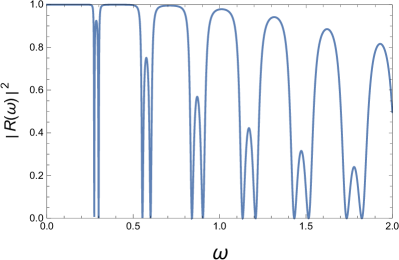
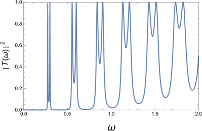
Figure 10: $|{R}_{3,eff}|^{2}$ and $|{T}_{3,eff}|^{2}$ with parameters $V_{1}=V_{2}=V_{3}=0.5$, $x_{1}=-10$, $x_{2}=-20$ and $x_{3}=-30$.

References

- [1] B. P. Abbott et al. [LIGO Scientific and Virgo Collaborations], Phys. Rev. Lett. 116, no. 6, 061102 (2016) [arXiv:1602.03837 [gr-qc]].
- [2] B. P. Abbott et al. [LIGO Scientific and Virgo Collaborations], Phys. Rev. Lett. 119, no. 16, 161101 (2017) [arXiv:1710.05832 [gr-qc]].
- [3] V. Cardoso, E. Franzin and P. Pani, Phys. Rev. Lett. 116, no. 17, 171101 (2016) [arXiv:1602.07309 [gr-qc]].
- [4] V. Cardoso and P. Pani, Nat. Astron. 1, no. 9, 586 (2017) [arXiv:1709.01525 [gr-qc]].
- [5] B. P. Abbott et al. [LIGO Scientific and Virgo Collaborations], Phys. Rev. Lett. 116, no. 22, 221101 (2016) [arXiv:1602.03841 [gr-qc]].
- [6] B. P. Abbott et al. [LIGO Scientific and Virgo Collaborations], arXiv:1811.00364 [gr-qc].
- [7] S. B. Giddings, Class. Quant. Grav. 33, no. 23, 235010 (2016) [arXiv:1602.03622 [gr-qc]].
- [8] S. B. Giddings, Nature Astronomy 1, Article number: 0067 (2017) [arXiv:1703.03387 [gr-qc]].
- [9] A. Almheiri, D. Marolf, J. Polchinski and J. Sully, JHEP 1302, 062 (2013) [arXiv:1207.3123 [hep-th]].
- [10] J. Maldacena and L. Susskind, Fortsch. Phys. 61, 781 (2013) [arXiv:1306.0533 [hep-th]].
- [11] S. D. Mathur, Fortsch. Phys. 53, 793 (2005) [hep-th/0502050].
- [12] P. O. Mazur and E. Mottola, Proc. Nat. Acad. Sci. 101, 9545 (2004) [gr-qc/0407075].
- [13] M. Visser and D. L. Wiltshire, Class. Quant. Grav. 21, 1135 (2004) [gr-qc/0310107].
- [14] Y. T. Wang, J. Zhang and Y. S. Piao, arXiv:1810.04885 [gr-qc].
- [15] S. L. Liebling and C. Palenzuela, Living Rev. Rel. 15, 6 (2012) [Living Rev. Rel. 20, no. 1, 5 (2017)] [arXiv:1202.5809 [gr-qc]].
- [16] R. Brito, S. Ghosh, E. Barausse, E. Berti, V. Cardoso, I. Dvorkin, A. Klein and P. Pani, Phys. Rev. Lett. 119, no. 13, 131101 (2017) [arXiv:1706.05097 [gr-qc]].
- [17] C. Palenzuela, P. Pani, M. Bezares, V. Cardoso, L. Lehner and S. Liebling, Phys. Rev. D 96, no. 10, 104058 (2017) [arXiv:1710.09432 [gr-qc]].
- [18] V. Cardoso, S. Hopper, C. F. B. Macedo, C. Palenzuela and P. Pani, Phys. Rev. D 94, no. 8, 084031 (2016) [arXiv:1608.08637 [gr-qc]].
- [19] E. Barausse, V. Cardoso and P. Pani, Phys. Rev. D 89, no. 10, 104059 (2014) [arXiv:1404.7149 [gr-qc]].
- [20] J. Abedi, H. Dykaar and N. Afshordi, Phys. Rev. D 96, no. 8, 082004 (2017) [arXiv:1612.00266 [gr-qc]].
- [21] R. H. Price and G. Khanna, Class. Quant. Grav. 34, no. 22, 225005 (2017) [arXiv:1702.04833 [gr-qc]].
- [22] H. Nakano, N. Sago, H. Tagoshi and T. Tanaka, PTEP 2017, no. 7, 071E01 (2017) [arXiv:1704.07175 [gr-qc]].
- [23] Z. Mark, A. Zimmerman, S. M. Du and Y. Chen, Phys. Rev. D 96, no. 8, 084002 (2017) [arXiv:1706.06155 [gr-qc]].
- [24] J. Zhang and S. Y. Zhou, Phys. Rev. D 97, no. 8, 081501 (2018) [arXiv:1709.07503 [gr-qc]].
- [25] P. Bueno, P. A. Cano, F. Goelen, T. Hertog and B. Vercnocke, Phys. Rev. D 97, no. 2, 024040 (2018) [arXiv:1711.00391 [gr-qc]].
- [26] Y. T. Wang, Z. P. Li, J. Zhang, S. Y. Zhou and Y. S. Piao, Eur. Phys. J. C 78, no. 6, 482 (2018) [arXiv:1802.02003 [gr-qc]].
- [27] M. R. Correia and V. Cardoso, Phys. Rev. D 97, no. 8, 084030 (2018) [arXiv:1802.07735 [gr-qc]].
- [28] Q. Wang and N. Afshordi, Phys. Rev. D 97, no. 12, 124044 (2018) [arXiv:1803.02845 [gr-qc]].
- [29] A. Testa and P. Pani, Phys. Rev. D 98, no. 4, 044018 (2018) [arXiv:1806.04253 [gr-qc]].
- [30] R. A. Konoplya, Z. Stuchl k and A. Zhidenko, Phys. Rev. D 99, no. 2, 024007 (2019) [arXiv:1810.01295 [gr-qc]].
- [31] A. Maselli, S. H. Volkel and K. D. Kokkotas, Phys. Rev. D 96, no. 6, 064045 (2017) [arXiv:1708.02217 [gr-qc]].
- [32] J. Westerweck et al., Phys. Rev. D 97, no. 12, 124037 (2018) [arXiv:1712.09966 [gr-qc]].
- [33] R. S. Conklin, B. Holdom and J. Ren, Phys. Rev. D 98, no. 4, 044021 (2018) [arXiv:1712.06517 [gr-qc]].
- [34] K. W. Tsang et al., Phys. Rev. D 98, no. 2, 024023 (2018) doi:10.1103/PhysRevD.98.024023 [arXiv:1804.04877 [gr-qc]].
- [35] A. B. Nielsen, C. D. Capano, O. Birnholtz and J. Westerweck, arXiv:1811.04904 [gr-qc].
- [36] R. K. L. Lo, T. G. F. Li and A. J. Weinstein, arXiv:1811.07431 [gr-qc].
- [37] Y. T. Wang, J. Zhang, S. Y. Zhou and Y. S. Piao, arXiv:1904.00212 [gr-qc].
- [38] B. Chen, Y. Chen, Y. Ma, K. L. R. Lo and L. Sun, arXiv:1902.08180 [gr-qc].
- [39] J. D. Bekenstein, Lett. Nuovo Cim. 11, 467 (1974).
- [40] J. D. Bekenstein and V. F. Mukhanov, Phys. Lett. B 360, 7 (1995) [gr-qc/9505012].
- [41] V. F. Foit and M. Kleban, Class. Quant. Grav. 36, no. 3, 035006 (2019) [arXiv:1611.07009 [hep-th]].
- [42] V. Cardoso, V. F. Foit and M. Kleban, arXiv:1902.10164 [hep-th].
- [43] E. Berti, V. Cardoso and A. O. Starinets, Class. Quant. Grav. 26, 163001 (2009) [arXiv:0905.2975 [gr-qc]].
- [44] R. Vicente, V. Cardoso and J. C. Lopes, Phys. Rev. D 97, no. 8, 084032 (2018) [arXiv:1803.08060 [gr-qc]].
- [45] E. Barausse, R. Brito, V. Cardoso, I. Dvorkin and P. Pani, Class. Quant. Grav. 35, no. 20, 20LT01 (2018) [arXiv:1805.08229 [gr-qc]].
- [46] S. M. Du and Y. Chen, Phys. Rev. Lett. 121, no. 5, 051105 (2018) [arXiv:1803.10947 [gr-qc]].