Dynamics of electron beams in the solar corona plasma with density fluctuations

The problem of beam propagation in a plasma with small scale and low intensity inhomogeneities is investigated. It is shown that the electron beam propagates in a plasma as a beam-plasma structure and is a source of Langmuir waves. The plasma inhomogeneity changes the spatial distribution of the waves. The spatial distribution of the waves is fully determined by the distribution of plasma inhomogeneities. The possible applications to the theory of radio emission associated with electron beams are discussed.

1 Introduction

One of the challenging problems in the theory of type III bursts, widely discussed in the literature, is the fine structure of the bursts. The fine structure is observed in almost all ranges of frequencies from GHz (Benz et al. (1982); Benz et al. (1996)) to a few tens of kHz in interplanetary space (Chaizy et al. (1995)). Direct observations of Langmuir waves and energetic electrons show that Langmuir waves have rather clumpy spatial distribution whereas the electron stream seems rather continuous (Lin et al. (1981); Chaizy et al. (1995)).

There are a few alternative ways to explain the observational data. The existing theories can be roughly divided into three groups in accordance with the electron beam density or the energy of the Langmuir waves. The first group of theories is based on the assumption that nonlinear instabilities of strong turbulence theory can suppress quasilinear relaxation (Papadopoulos, Goldstein & Smith (1974)) and lead to extreme clumpiness of the spatial distribution of Langmuir waves (Thejappa & MacDowall (1998)). However, some observations and theoretical studies (Cairns & Robinson (1995)) raise doubts as to whether the Langmuir turbulence level is high enough for strong-turbulence processes. The second, recently developed group of theories, is based on the prediction that an electron beam propagates in a state close to marginal stability, i.e. one where the fluctuation-dependent growth rate is compensated for by the damping rate (Robinson (1992); Robinson & Cairns (1993)). In this view, the growth rate of beam-plasma instability is perturbed by the ambient density fluctuations (Robinson (1992)). The third, more traditional group of theories, considers the beam propagation in the limit of weak turbulence theory (Ryutov & Sagdeev (1970); Takakura & Shibahashi (1976); Magelssen and Smith (1977); Takakura (1982); Grognard (1985)). The basic idea is that the electron beam generates Langmuir waves at the front of the electron stream and the waves are absorbed at the back of the stream, ensuring electron propagation over large distances. However, this idea was not proved for a long time (Melrose (1990)). Recently Mel’nik has demonstrated analytically (Mel’nik (1995)) that a mono-energetic beam can propagate as a beam-plasma structure (BPS). This result has been confirmed numerically (Kontar, Lapshin & Mel’nik (1998)) and applied to the theory of type III bursts (Mel’nik, Lapshin & Kontar (1999)). The solution obtained (Mel’nik & Kontar (2000)) directly resolves Sturrock’s dilemma (Sturrock (1964)) and may explain the almost constant speed of type III sources. However, the influence of plasma inhomogeneity on the dynamics of a BPS has never been studied although the correlation between Langmuir wave clumps and density fluctuations demonstrates the importance of such considerations (Robinson, Cairns & Garnett (1992)).

The influence of plasma inhomogeneity on Langmuir waves and beam electrons has been studied from various points of view. An account of plasma inhomogeneities may explain why accelerated beam electrons appear in the experiments with quasilinear relaxation of an electron beam (Ryutov (1969)). Relativistic dynamics of an electron beam with random inhomogeneities, as applied to laboratory plasmas, was considered in (Hishikawa & Ryutov (1976)). It has been shown (Muschietti, Goldman & Newman (1985)) that the solar corona density fluctuations may be extremely effective in quenching the beam-plasma instability. Moreover, the isotropic plasma inhomogeneities may lead to efficient isotropisation of plasma waves (Goldman & DuBois (1982)) whereas those alongated along the direction of ambient magnetic field have little influence on the beam stability. Therefore, the growth rate of beam-plasma instability was postulated to be very high in the regions of low amplitude density fluctuations (Melrose, Dulk & Cairns (1986); Melrose & Goldman (1987)). Isotropic density fluctuations of ambient plasma density were also employed to explain low level of Langmuir waves in microbursts (Gopalswamy (1993)).

In this paper the dynamics of a spatially limited electron cloud is considered in a plasma with small scale density fluctuations. In the treatment presented here, quasilinear relaxation is a dominant process and density inhomogeneities are too weak to suppress the instability. Indeed, observations of interplanetary scintillations from extragalactic radio sources (Cronyn (1972)) lead to an average value of $\Delta n/n$ of the order of $10^{-3}$ (Smith & Sime (1979)). Nevertheless, the low intensity density fluctuations lead to significant spatial redistribution of wave energy. The numerical results obtained demonstrate that electrons propagate as a continuous stream while the Langmuir waves generated by the electrons are clumpy. Both electrons and Langmuir waves propagate in a plasma as a BPS with an almost constant velocity. However, density fluctuations lead to some energy losses.

2 Electron beam and density fluctuations

The problem of one-dimensional electron beam propagation is considered in a plasma with density fluctuations. The one-dimensional character of electron beam propagation is supported by the 3D numerical solution of the kinetic equations (Churaev & Agapov (1980)) and additionally by the fact that in the case of type III bursts electrons propagate along open magnetic field lines (Suzuki & Dulk (1985)).

2.1 Electron beam

There is still uncertainty in the literature as to whether electron beams are strong enough to produce strong turbulence or whether the beam is so rarified that quasilinear relaxation is suppressed by damping or scattering. While some observations are in favor of the strong turbulence regime (Thejappa & MacDowall (1998)) others are interpreted as implying marginal stability (Cairns & Robinson (1995)). Therefore, we consider the intermediate case of a medium density beam, which is not strong enough to start strong turbulence processes,

$$W/nT\ll(k\lambda_{D})^{2},$$ (1)

but is dense enough to make quasilinear relaxation a dominant process. Here $W$ is the energy density of Langmuir waves generated by the beam, $T$ is the temperature of the surrounding plasma, $k$ is the wave number, and $\lambda_{D}$ is the electron Debye length.

The initial value problem is solved with an initially-unstable electron distribution function, which leads to the formation of a BPS in the case of homogeneous plasma (Mel’nik & Kontar (2000))

$$f(v,x,t=0)=g_{0}(v)\mbox{exp}(-x^{2}/d^{2}),$$ (2)

where

$$g_{0}(v)=\left\{\begin{array}[]{ll}\displaystyle\frac{2n^{\prime}v}{v_{0}^{2}},&\mbox{$v<v_{0}$},\\ 0,&\mbox{$v>v_{0}$}.\end{array}\right.$$ (3)

Here $d$ is the characteristic size of the electron cloud and $v_{0}$ is the velocity of the electron beam. The initial spectral energy density of Langmuir waves

$$W(v,x,t=0)\simeq\frac{T}{2\pi^{2}\lambda_{D}^{2}},$$ (4)

is of the thermal level and uniformly distributed in space. The electron temperature of the corona is taken to be $T=10^{6}$K, which gives an electron thermal velocity $v_{Te}=\sqrt{3kT/m}\simeq 6.7\times 10^{8}$cm s^-1.

2.2 Ambient density fluctuations

Following common practice in the literature on plasma inhomogeneity Langmuir waves are treated in the approximation of geometrical optics (the WKB approximation) when the length of a Langmuir wave is much smaller than the size of the plasma inhomogeneity (Vedenov, Gordeev & Rudakov (1967); Ryutov (1969))

$$\lambda\ll L,$$ (5)

where

$$L\equiv\left(\frac{1}{\omega_{pe}}\frac{\partial\omega_{pe}}{\partial x}\right)^{-1},$$ (6)

is the scale of ambient plasma density fluctuations, and $\omega_{pe}$ is the local electron plasma frequency. The plasma inhomogeneity changes the dispersion properties of Langmuir waves and if the intensity of density fluctuations is small then the dispersion relation can be written

$$\omega(k,x)=\omega_{pe}\left[1+\frac{1}{2}\frac{\Delta n}{n}+\frac{3k^{2}v_{Te}^{2}}{2\omega_{pe}^{2}}\right],$$ (7)

where $v_{Te}$ is the electron thermal velocity. The intensity of the density fluctuations should be small (Coste et al. (1975))

$$\frac{\Delta n}{n}<\frac{3k^{2}v_{Te}^{2}}{\omega_{pe}^{2}},$$ (8)

to ensure that the corresponding fluctuations of local plasma frequency are within the thermal width of plasma frequency. Thus, for the typical parameters of the corona plasma (plasma density $n=5\times 10^{8}$cm^-3 or plasma frequency $f_{p}=\omega_{pe}/2\pi\approx 200.73$MHz), and assuming a beam velocity $v_{0}=10^{10}$cm s^-1, the density fluctuations are limited to $\Delta n/n<10^{-2}$.

2.3 Quasilinear equations

In the case of weak turbulence theory (1), and under the conditions of the WKB approximation (5,8), the evolution of the electron distribution function $f(v,x,t)$ and the spectral energy density $W(v,x,t)$ are described by the system of kinetic equations (Ryutov (1969))

$$\frac{\partial f}{\partial t}+v\frac{\partial f}{\partial x}=\frac{4\pi^{2}e^{2}}{m^{2}}\frac{\partial}{\partial v}\frac{W}{v}\frac{\partial f}{\partial v},$$ (9)

and

$$\frac{\partial W}{\partial t}+\frac{\partial\omega}{\partial k}\frac{\partial W}{\partial x}-\frac{\partial\omega_{pe}}{\partial x}\frac{\partial W}{\partial k}=\frac{\pi\omega_{pe}}{n}v^{2}W\frac{\partial f}{\partial v},\;\omega_{pe}=kv,$$ (10)

where $\partial\omega/\partial k=3v_{Te}^{2}/v$ is the group velocity of Langmuir waves, and $W(v,x,t)$ plays the same role for waves as the electron distribution function does for particles. The system (9,10) describes the resonant interaction $\omega_{pe}=kv$ of electrons and Langmuir waves. On the right-hand side of equations (9,10) I omit the spontaneous terms due to their small magnitude relative to the induced ones (Ryutov & Sagdeev (1970)).

The presence of a local plasma frequency gradient leads to two physical effects on the kinetics of the Langmuir waves (10). Firstly, the characteristic time of the beam-plasma interaction depends on the local density and therefore the resonance condition for the plasmons may itself change during the course of beam propagation. Secondly, the Langmuir wave propagating in the inhomogeneous plasma experiences a shift of wavenumber $\Delta k(x)$, due to the variation of the local refractive index. The second effect has been shown to have the main impact on Langmuir wave kinetics whereas the first effect can be neglected (Coste et al. (1975)).

Thus, we are confronted with the initial value problem of electron cloud propagation in a plasma with density fluctuations. The problem is nonlinear and is characterized by three different time scales. The fastest process in the system is the quasilinear relaxation, on the quasilinear timescale $\tau\approx n/n^{\prime}\omega_{pe}$. The second timescale is that of processes connected with plasma inhomogeneity. Thirdly, there is the timescale of an electron cloud propagation in a plasma that significantly exceeds all other timescales.

3 Quasilinear relaxation and plasma inhomogeneity

The main interaction in the system is beam – wave interaction governed by the quasilinear terms on the right hand side of equations (9,10) . It is well-known that the unstable electron distribution function (3) leads to the generation of plasma waves. The result of quasilinear relaxation for an electron beam homogeneously distributed in space is a plateau of the electron distribution function (Ryutov & Sagdeev (1970))

$$\displaystyle f(v,t\approx\tau)=\left\{\begin{array}[]{ll}\displaystyle\frac{n^{\prime}}{v_{0}},&\mbox{$v<v_{0}$}\\ 0,&\mbox{$v>v_{0}$}\end{array}\right.$$ (13)

and the spectral energy density

$$\displaystyle W(v,t\approx\tau)=\displaystyle\frac{mn^{\prime}}{v_{0}\omega_{pe}}\int_{0}^{v}\left(1-\frac{v_{0}}{n^{\prime}}g_{0}(v)\right)dv,\;\;v<v_{0}$$ (14)

where $g_{0}(v)$ is the initial distribution function of the beam.

In the case of an inhomogeneous plasma we can also consider relaxation of a homogeneously distributed beam. Thus, the kinetic equations (9,10) will take the form

$$\frac{\partial f}{\partial t}=\frac{4\pi^{2}e^{2}}{m^{2}}\frac{\partial}{\partial v}\frac{W}{v}\frac{\partial f}{\partial v},$$ (15)

and

$$\frac{\partial W}{\partial t}+\frac{v^{2}}{L_{0}}\frac{\partial W}{\partial v}=\frac{\pi\omega_{pe}}{n}v^{2}W\frac{\partial f}{\partial v},\;\;\;\omega_{pe}=kv,$$ (16)

where the transport terms are omitted. Here, the inhomogeneity scale is also assumed to be constant and equal to $L_{0}$. It should be noted that this assumption is physically incorrect. The change in the spectrum of the Langmuir waves is due solely to the spatial movement of the waves with the group velocity. However, from a mathematical point of view, it is well justified as the group velocity of Langmuir waves is small ($3v_{Te}^{2}/v\ll v$) and effects connected with wave transport can be neglected.

Equations (15,16) describe two physical effects: quasilinear relaxation (with characteristic time $\tau$) and the drift of Langmuir waves in velocity space (the characteristic time $\tau_{2}=|L_{0}|/v$. Since $\tau_{2}\gg\tau$ the influence of plasma inhomogeneity can be considered as the evolution of the final stage of quasilinear relaxation. Two possible cases of plasma density change are considered: plasma density decreasing ($L_{0}<0$) with distance and plasma density increasing ($L_{0}>0$) with distance.

3.1 Plasma density decreasing with distance

In this case $L_{0}$ is negative. After the time of quasilinear relaxation, a plateau is established in the electron distribution function and a high level of Langmuir waves is generated. Since the quasilinear processes are fast we have a plateau at every moment of time

$$\displaystyle f(v,t\approx\tau)=\left\{\begin{array}[]{ll}\displaystyle\frac{n^{\prime}}{v_{0}},&\mbox{$v<v_{0}$}\\ 0,&\mbox{$v>v_{0}$}\end{array}\right.$$ (19)

The wave spectrum is changing with time, and from the fact that we have a plateau at every moment equation (16) can be reduced to

$$\frac{\partial W}{\partial t}-\frac{v^{2}}{|L_{0}|}\frac{\partial W}{\partial v}=0$$ (20)

The role of initial wave distribution is played by the spectral energy density generated during the relaxation stage (14). Integrating equation (20) we obtain the solution for $t\gg\tau$

$$W(v,t)=\frac{m}{\omega_{pe}}(1/v-t/|L_{0}|)^{-3}\;\;\;\;\;\;\;\;\;\;\;\;\;\;\;\;\;\;\;\;\;\;\;\;\;\;\;\;\;\;\;\;\;$$ (21)

$$\;\;\;\times\int_{0}^{1/(1/v-t/|L_{0}|)}\left[\frac{n^{\prime}}{v_{0}}-g_{0}(v)\right]dv,\;\;v<u(t)$$ (22)

where

$$u(t)=\frac{v_{0}}{1+v_{0}t/|L_{0}|}$$ (23)

is the maximum velocity of the Langmuir waves. Note, that the electron distribution function is constant and presents a plateau (19).

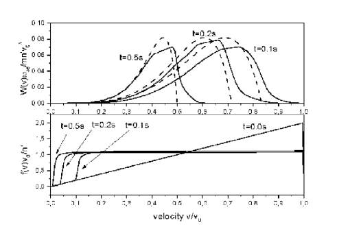
Figure 1: The electron distribution function $f(v,t)$ and the spectral energy density of Langmuir waves $W(v,t)$ at various times, for the case where the plasma density decreases with distance, $L_{0}=-5\times 10^{9}$cm. Numerical solution of kinetic equations (15,16) $n^{\prime}=100$cm^-3, $v_{0}=1.0\times 10^{10}$cm s^-1.

The numerical solution of equations (15,16) with the initial electron distribution function (3) is presented in fig. 1. Comparing the numerical results and the simplified solution (21) we see a good agreement (see fig. 1). The plateau for a wide range of velocities is formed after a short time, $t=0.1$s, and it remains almost unchanged up to the end of the calculation. For the time $t>0.1$s, the drift of the Langmuir wave spectrum toward smaller phase velocities becomes observable. At $t=0.5$s, the maximum phase velocity is half of the initial beam velocity.

3.2 Plasma density increasing with distance

An increasing plasma density leads to a shift toward larger phase velocities. For $v>v_{0}$ we have a negative derivative at the edge of the electron distribution function, and electrons absorb waves with the corresponding phase velocities. Absorption of waves then leads to acceleration of particles. This process continues until all the waves generated during the beam relaxation are absorbed by the electrons.

In the case of increasing density we are unable to find an exact solution, but we can find the solution for $t\rightarrow\infty$. Using conservation of energy (Ryutov (1969))

$$\omega_{pe}\int_{0}^{u(t)}\frac{W(v,t)}{v^{2}}dv+\int_{0}^{u(t)}\frac{mn^{\prime}}{2u(t)}v^{2}dv$$ (24)

$$=\frac{m}{2}\int_{0}^{v_{0}}g_{0}(v)v^{2}dv$$ (25)

and that the fact $W(v,t)=0$ at $t\rightarrow\infty$ we can find the maximum velocity for the initial distribution function (3)

$$u(t\rightarrow\infty)=\sqrt{3/2}v_{0}$$ (26)

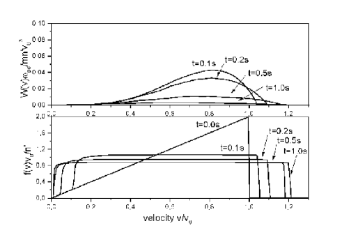
Figure 2: The electron distribution function $f(v,t)$ and the spectral energy density of Langmuir waves $W(v,t)$ at various times for the case where the plasma density increases with distance, $L_{0}=5\times 10^{9}$cm. Numerical solution of kinetic equations (15,16) $n^{\prime}=100$cm^-3, $v_{0}=1.0\times 10^{10}$cm s^-1.

As predicted, the numerical solution tends to the maximum velocity $\approx 1.22v_{0}$ (fig. 2). As in the previous case, at $t=0.1$s we have the result of quasilinear relaxation - a plateau in the electron distribution function and a high level of Langmuir waves. For times $t>0.1$s, the drift of Langmuir waves and consequent acceleration of electrons is observable. At $t=1$s almost all plasma waves are observed near the leading edge of the plateau and the maximum plateau velocity is close to the value given by (26).

4 Propagation of an electron cloud

In this section the numerical results of the evolution of the electron beam in the plasma with density fluctuations are presented. We begin with the case where the ambient density fluctuations in the plasma are periodic and sine-like. The dependency of plasma density on distance is

$$n(x)=n_{0}(1+\alpha\mbox{sin}(x/\Delta x))$$ (27)

where $\Delta x$ defines the period of the density fluctuations and $\alpha n_{0}$ is the amplitude of the density irregularities. The background plasma density is taken as a typical value for the starting frequencies of type III bursts $n_{0}=5\times 10^{8}$ cm^-3, corresponding to a local plasma frequency $f_{p}=\omega_{pe}/2\pi=200.73$MHz. As noted, small-intensity density fluctuation are considered, i.e. the local plasma frequency change due to the inhomogeneity is less than the thermal width of the plasma frequency (8). The value $\alpha$ is taken to be $10^{-3}$, which is considered to be a typical value for solar coronal observations (Cronyn (1972); Smith & Sime (1979)). The spatial period of the plasma fluctuations $\Delta x=d/12$ is taken to be less than the initial size of the electron cloud. Thus, we have regions of size $\pi d/12\approx 0.26d$ with positive and negative density gradients. Recently, it has been shown that an electron beam can propagate in a homogeneous plasma as a BPS (Mel’nik, Lapshin & Kontar (1999); Mel’nik, Kontar & Lapshin (2000); Mel’nik & Kontar (2000)). Therefore, it is important to consider the dynamics of the electron beams at distances greatly exceeding the size of the electron cloud.

4.1 Initial evolution of the electron beam and formation of a BPS

At the initial time $t=0$ we have an electron distribution function which is unstable. Due to fast quasilinear relaxation, electrons form a plateau in the electron distribution function and generate a high level of plasma waves. At time $t=0.1$s, the typical result of quasilinear relaxation is observed. The electron distribution function and the spectral energy density evolve in accordance with the gas-dynamic solution (Mel’nik (1995); Mel’nik & Kontar (2000))

$$\displaystyle f(v,x,t)=\left\{\begin{array}[]{ll}\displaystyle\frac{n^{\prime}}{v_{0}}\mbox{exp}\left(-\frac{(x-v_{0}t/2)^{2}}{d^{2}}\right),&\mbox{$v<v_{0}$}\\ 0,&\mbox{$v>v_{0}$}\end{array}\right.$$ (30)

$$W(v,x,t)=\frac{mn^{\prime}}{v_{0}\omega_{pe}}v^{4}\left[1-\frac{v}{v_{0}}\right]\;\;\;\;\;\;\;\;\;\;\;\;\;\;\;\;\;\;\;\;\;\;\;\;\;\;\;$$ (31)

$$\;\;\;\;\;\;\;\;\;\;\;\;\;\;\;\;\;\;\;\;\;\;\times\mbox{exp}\left(-\frac{(x-v_{0}t/2)^{2}}{d^{2}}\right),\;\;v<v_{0}$$ (32)

At this stage the influence of the plasma inhomogeneity is not observable.

The numerical solution of the kinetic equations and the gas-dynamic solution show that electrons propagate in a plasma accompanied by a high level of plasma waves. Since the plasma waves exist at a given point for some time, while the structure passes this point, the spectrum of the waves should change due to the wave movement. To understand the physics of the process we consider the evolution of the electron distribution function and the spectral energy density of Langmuir waves at a given point.

4.2 The electron distribution function and the spectral energy density of plasma waves

At every spatial point we observe two physical processes. The first process is connected with the spatial movement of a BPS, as would be the case for a homogeneous plasma (Mel’nik, Kontar & Lapshin (2000); Mel’nik & Kontar (2000)). The second process is the influence of plasma inhomogeneity on the Langmuir waves. Depending on the sign of the density gradient, the Langmuir wave spectrum takes on a different form.

Consider the time evolution of the electron distribution function and the spectral energy density of Langmuir waves at two close points $x=15.2d$ and $x=15.47d$ (see fig. 3). The first point is chosen in the region with increasing density and the second in the region where the density decreases with distance. The first particles arrive to these points at approximately $t\sim 1.9$s. The arriving electrons form a plateau in the electron distribution function and generate a high level of plasma waves for the time of quasilinear relaxation $\tau\approx 0.01$ s.

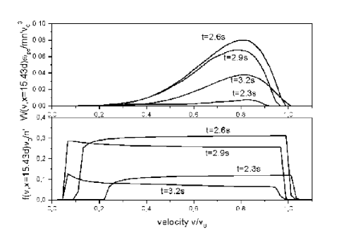
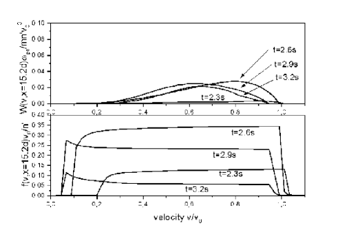
Figure 3: The electron distribution function $f(v,x,t)$ and the spectral energy density of Langmuir waves $W(v,x,t)$ at $x=15.2d$ and at $x=15.47d$. Numerical solution of kinetic equations for a plasma with sine-like density fluctuations (27) $n^{\prime}=100$cm^-3, $v_{0}=1.0\times 10^{10}$cm s^-1.

The movement of the particles leads to the growth of the plateau height at the front of the structure for $1.9\mbox{ s}<t<2.7\mbox{ s}$. Due to the fact that at the front of the structure electrons come with a positive derivative, $\partial f/\partial v>0$, the level of plasma waves also increases. When the peak of the plateau height is reached at $t\approx 2.7$s the reverse process takes place. The plateau height decreases and the arriving electrons have a negative derivative $\partial f/\partial v<0$ that leads to absorption of waves. The growth and decrease of the plateau height and the level of plasma waves is typical for a homogeneous plasma (Mel’nik & Kontar (2000)). However, while the structure passes a given point the spectrum of Langmuir waves experiences the change. This change depends on the sign of the plasma density gradient. In the region with decreasing density ($x=15.47d$) the Langmuir waves have a negative shift in velocity space while the growing plasma density ($x=15.2d$) supplies a positive shift in phase velocity of the plasma waves. At the point with the positive gradient, the Langmuir waves shifted in phase velocity space are effectively absorbed by the electrons while the negative plasma gradient does not lead to the absorption of waves. This behavior results in different levels of plasma waves at two very close points with the opposite density-gradient sign.

Figure 3 demonstrates the existence of accelerated electrons with $v>v_{0}$. These electrons are accelerated by Langmuir waves in the regions with positive plasma-density gradient. Electrons with velocity larger than the initial beam velocity have been observed in laboratory plasma experiments. This effect was also considered from an analytical standpoint by (Ryutov (1969)) in application to laboratory plasmas.

4.3 Dynamics of electrons and accompanying Langmuir waves

The processes of wave generation at the front and absorption at the back take place at every spatial point and therefore the structure can travel over large distances, being the source of plasma waves (Kontar, Lapshin & Mel’nik (1998); Mel’nik, Lapshin & Kontar (1999); Mel’nik & Kontar (2000)).

At time $t=5.0$s, electrons accompanied by Langmuir waves have passed over a large distance but the general physical picture remains the same (fig. 4). Generally, electrons and Langmuir waves propagate as a BPS. At every spatial point electrons form a plateau at the electron distribution function and we have a high level of plasma waves. The electron cloud has a maximum of the electron density at $x=27d$. Plasma waves are also concentrated in this region and the maximum of Langmuir wave density is located at the maximum of electron density $x=27d$. The spectrum of Langmuir waves has a maximum close to $v\approx 0.8v_{0}$. The spatial profile, averaged over the plasma inhomogeneity period, is close to the result obtained for a homogeneous plasma.

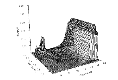
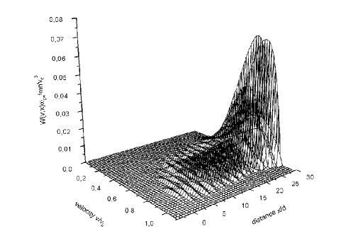
Figure 4: The electron distribution function $f(v,x,t)$ and the spectral energy density of Langmuir waves $W(v,x,t)$ at $t=5.0$s. Numerical solution of the kinetic equations with sine-like density fluctuations (27) $n^{\prime}=100$cm^-3, $v_{0}=1.0\times 10^{10}$cm s^-1.

However, the spatial profile of Langmuir waves has a fine structure that can be seen in fig. 5. The Langmuir waves are grouped into clumps (the regions with high level of plasma waves, following the terminology of (Smith & Sime (1979))). The size of a clump is determined by the spatial size of the density fluctuations and is equal to half of the density fluctuation period $\pi d/12\approx 0.26d$. The maxima of Langmuir wave density are located in regions of negative plasma-density gradient and the regions with low levels of Langmuir turbulence are where the density gradient is positive.

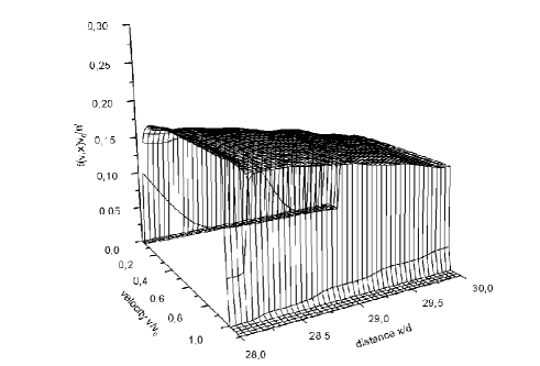
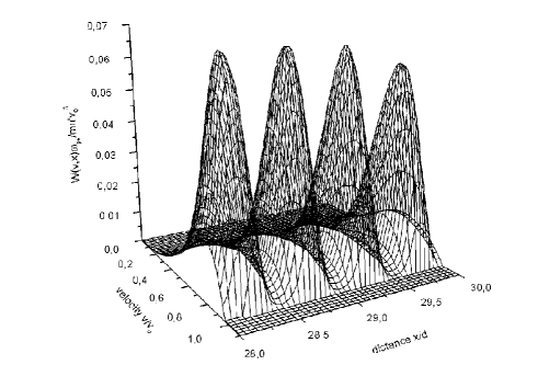
Figure 5: Detailed picture of the electron distribution function $f(v,x,t)$ and the spectral energy density of Langmuir waves $W(v,x,t)$ at $t=5.0$s. Numerical solution of kinetic equations with sine-like density fluctuations (27) $n^{\prime}=100$cm^-3, $v_{0}=1.0\times 10^{10}$cm s^-1.

The other interesting result is that while the Langmuir wave distribution is determined by the irregularities of ambient plasma the electron distribution function is a smooth function of distance (see fig. 5). The electrons in the structure propagate as a continuous stream, being slightly perturbed by the density fluctuations. The influence of plasma inhomogeneity on electron distribution is observed in the appearance of accelerated particles with $v>v_{0}$ and the fact that the maximum plateau velocity is slightly decreasing with time during the course of beam-plasma passing a given point (fig. 3). The accelerated electrons tend to accumulate at the front of the structure and the electrons decelerated concentrate at the back of the structure.

4.4 The energy distribution of waves

The energy distribution of waves

$$E_{w}(x,t)=\int_{0}^{\infty}Wdk=\omega_{pe}\int_{0}^{v_{0}}\frac{W(v,x,t)}{v^{2}}dv$$ (33)

is presented in fig. 6, where $E_{0}=mn^{\prime}v_{0}^{2}/4$ is the initial beam energy. The energy distribution explicitly shows the correlation between the plasma and wave energy-density fluctuations. The regions of decreasing plasma density have higher levels of Langmuir turbulence than the corresponding regions with increasing plasma density. The energy distribution of waves appears to be modulated by the ambient plasma density fluctuations. On the other hand, the wave energy density distribution averaged over the period of density fluctuations has a spatial profile close to that in a homogeneous plasma. The maximum of wave energy together with the maximum of electron density propagate with the constant velocity $\approx 0.5v_{0}$.

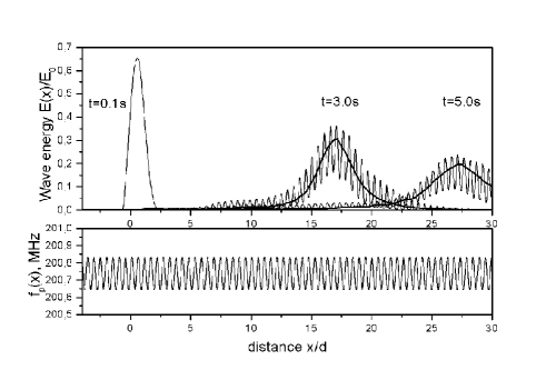
Figure 6: The energy density of plasma waves $E(x)$ at various times and the local plasma frequency $f_{p}(x)$ (27) as a function of distance at various times. The bold line shows the numerical solution for homogeneous plasma. Numerical solution of kinetic equations $n^{\prime}=100$cm^-3, $v_{0}=1.0\times 10^{10}$cm s^-1.

The other physical effect that should be noted is the energy losses by the structure in the form of Langmuir waves. In figs. 4,6 we see that there is a small but non-zero level of plasma waves behind the beam-plasma structure. These waves are also concentrated into clumps in the regions where the plasma gradient is negative. To explain why the structure leaves the plasma waves we note the negative shift in phase velocity of Langmuir waves in the regions with a decreasing density. Due to this shift we have more waves with low phase velocity than the electrons are able to absorb at the back. As a result the low velocity waves form a ”trace” of the structure (Kontar (2001)).

As was discussed previously, the quasilinear time is small but finite value. Therefore, the BPS experiences spatial expansion (Kontar, Lapshin & Mel’nik (1998)). The initial width-at-half-height of the structure is less than $2d$ whereas the spatial width of the structure at $t=5.0$s is about $5d$. Most of the energy and the majority of particles are concentrated within the width of the structure. Since the quasilinear time depends on the beam density, the quasilinear time for the particles far from the center of the structure is much larger than for the structure electrons. In these regions we can observe the situation where the influence of the plasma inhomogeneity is comparable with the quasilinear time. Indeed, in the tail of the structure we have regions with zero level of waves (where the Langmuir waves are absorbed by electrons when the plasma density increases) and regions with Langmuir waves (where plasma density is decreasing).

4.5 Pseudo-random fluctuations of density

There is special interest in the case where the density fluctuations are random, which looks like the case for a solar coronal plasma. A pseudo-random distribution of density fluctuations can be easily built by summing $N$ sine-like perturbations with random amplitude, phase, and period

$$n(x)=n_{0}(1+\sum\limits_{i=1}^{N}\alpha_{i}\mbox{sin}(x/\Delta x_{i}+\varphi_{i}))$$ (34)

where $n_{0}\alpha_{i}$, $\Delta x_{i}$, $\varphi_{i}$ are the amplitude, period and phase of a given sine-like density oscillations respectively. The values are chosen in the range to ensure the applicability of the kinetic equations. Thus, $0<\alpha_{i}\leq 0.001$, $d/2\leq\Delta x_{i}\leq d/12$, $0<\varphi_{i}\leq 2\pi$, $N=10$ are taken for the numerical calculations. The resulting density profile can be seen in fig. 7.

The spatial distribution of waves has now more complex structure (fig. 7). However, all the main results obtained for sine-like density fluctuations are also observed for pseudo-random density fluctuations (34). Firstly, the electron stream propagates in a plasma as a BPS. Secondly, observing the energy density profile of Langmuir waves one can see the clumps of Langmuir waves. The size of the clumps is determined by the size of the regions with negative density gradient. The electron distribution function of beam electrons remains smooth as in the previous case with sine-like density oscillations.

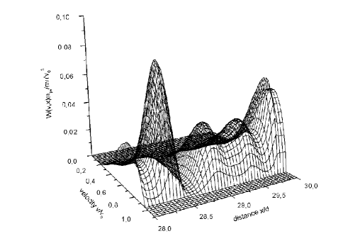
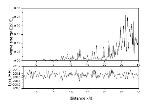
Figure 7: The spectral energy density of Langmuir waves $W(v,x,t)$, the energy density of plasma waves $E(x)$ at $t=5.0$s, and the local plasma frequency $f_{p}(x)$ (34) as functions of distance. Numerical solution of kinetic equations with random density fluctuations (34) $n^{\prime}=100$cm^-3, $v_{0}=1.0\times 10^{10}$cm s^-1.

The dependence of wave energy density on the amplitude of the density fluctuations is of special interest. From equation (10) it follows that a Langmuir wave propagating with the group velocity $v_{gr}=3v_{Te}^{2}/v$ over the distance $\Delta l$ experiences a shift of phase velocity

$$\Delta v\approx\frac{v^{2}}{Lv_{gr}}\Delta l.$$ (35)

Using the density profile (27) and estimating $L\approx\Delta l/\alpha$ one derives that

$$\frac{\Delta v}{v}\approx\frac{1}{3}\left(\frac{v}{v_{Te}}\right)^{2}\alpha$$ (36)

where we obtain, for our parameters, a phase velocity shift $\leq 0.1v$. Expression (36) also demonstrates that the shift of the wave phase velocity linearly depends on the amplitude of the density fluctuations. Therefore, in the case with an arbitrary amplitude of the density fluctuations, the higher the amplitude of the plasma inhomogeneity the larger the variations of the wave energy distribution. This tendency can be observed in fig. 7.

5 Main results and discussion

From a physical point of view it is interesting to consider the physical processes which lead to the reported results. As we see, the main physical effect, which leads to a complex spatial distribution of waves, is the shift of the phase velocity $\Delta v$ due to the wave movement. The growth rate of beam-plasma instability

$$\gamma(x)=\frac{\pi\omega_{pe}}{n}v^{2}\frac{\partial f}{\partial v},$$ (37)

also depends on distance. However, this dependency of the instability increment on local plasma density is negligible. At every spatial point we have a plateau with $\partial f/\partial v\approx 0$ and the value of $\partial f/\partial v$ is determined by the dynamics of a BPS not by the local plasma density. Therefore, the shift in phase velocity dominates the effect of instability increment dependency on distance. Indeed, if we manually exclude the terms connected with the velocity shift of the Langmuir waves, the spatial profile of waves will become smooth and the solution will be close to that obtained in the case of uniform plasma. This result agrees well with the qualitative results of (Coste et al. (1975)).

For application to the theory of type III bursts, special interest is presented by a combination of the two main properties of the solutions.

On one hand, the electron beam can propagate in a plasma over large distances, and is a source of a high level of Langmuir waves. A portion of these Langmuir waves can easily be transformed into observable radio emission via nonlinear plasma processes (Ginzburg & Zheleznyakov (1958)). At a scale much greater than the size of the beam, electrons and Langmuir waves propagate as a BPS that may be the source of type III bursts. The BPS propagates in inhomogeneous plasma with velocity $\approx v_{0}/2$ that can explain the almost-constant speed of the type III source. The finite size of the structure, the spatial expansion of the structure, and conservation of the particle number, are promising results for the theory of type III bursts.

On the other hand, plasma inhomogeneity brings additional results. The spatial distribution of Langmuir wave energy is extremely spikey and the distribution of waves is fully determined by the fluctuations of the ambient plasma density. This fact is in good agreement with satellite observations (Robinson, Cairns & Garnett (1992)). Moreover, following the plasma emission model, one obtains the fine structure of the radio emission.

At distances about $1$AU the quasilinear time might have a large value and the characteristic time of a wave velocity shift could be comparable to the quasilinear time. Therefore, the region of growing plasma density may lead to the suppression of quasilinear relaxation, whereas, in regions with a decreasing density, relaxation is found. Thus the Langmuir waves might be generated in only those spatial regions where the plasma gradient is less than or equal to zero. Indeed, in the tails of a beam-plasma structure the electron beam density is low and Langmuir waves are only observed in certain regions with non-positive density gradient.

6 Summary

In this paper the dynamics of a spatially bounded electron beam has been considered. Generally, the solution of the kinetic equations present a BPS. The structure moves with approximately constant velocity $\approx v_{0}/2$ and tends to conserve the number of particles. As in case of uniform plasma, electrons form a plateau and generate a high level of plasma waves at every spatial point.

However, small-scale inhomogeneity in the ambient plasma leads to significant changes in the spatial distribution of Langmuir waves. It is found that low intensity oscillations perturb the spatial distribution of Langmuir waves whereas the electron distribution function remains a smooth function of distance. The other interesting fact is that the distribution of waves is determined by the distribution of plasma inhomogeneities. The energy density of Langmuir waves has maxima and minima in the regions with positive and negative density gradient respectively.

Nevertheless, more detailed analysis is needed. One needs to include radio emission processes in order to calculate the observational consequences of the model in greater detail. The other challenge is the detailed comparison of such numerical results with satellite observations near the Earth’s orbit.