C-MIL: Continuation Multiple Instance Learning for
Weakly Supervised Object Detection

Abstract

Weakly supervised object detection (WSOD) is a challenging task when provided with image category supervision but required to simultaneously learn object locations and object detectors. Many WSOD approaches adopt multiple instance learning (MIL) and have non-convex loss functions which are prone to get stuck into local minima (falsely localize object parts) while missing full object extent during training. In this paper, we introduce a continuation optimization method into MIL and thereby creating continuation multiple instance learning (C-MIL), with the intention of alleviating the non-convexity problem in a systematic way. We partition instances into spatially related and class related subsets, and approximate the original loss function with a series of smoothed loss functions defined within the subsets. Optimizing smoothed loss functions prevents the training procedure falling prematurely into local minima and facilitates the discovery of Stable Semantic Extremal Regions (SSERs) which indicate full object extent. On the PASCAL VOC 2007 and 2012 datasets, C-MIL improves the state-of-the-art of weakly supervised object detection and weakly supervised object localization with large margins .

1 Introduction

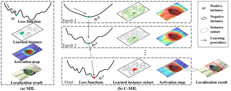
Figure 1: Comparison of MIL-based and C-MIL-based WSOD approaches. Due to the non-convex loss function MIL often falls into local minima and falsely localizes an object part. By introducing the continuation optimization with a series of smoothed loss functions, C-MIL alleviates the non-convexity problem and localizes full object extent. (Best viewed in color)

Weakly supervised object detection (WSOD) is rapidly gaining attention in computer vision area. WSOD approaches only require image category annotations indicating the presence or absence of a category of objects in images, significantly reducing human involvement by omitting labor-intensive bounding-box annotations [6, 27, 40, 12, 28, 29].

Despite extensive research over the past five years, WSOD remains an open problem, as indicated by the large performance gap ($\sim$ 20%) between WSOD [34, 37, 38] and fully supervised detection approaches [30, 17] on the PASCAL VOC detection benchmark [25].

Combined with deep neural networks, MIL has been the main WSOD method [8, 34]. However, it is observed that the model is prone to activate object parts instead of full object extent, particularly during the early learning epochs, Fig. 1(a). This phenomenon arises from non-convexity of the objective/loss functions. Optimizing such functions can get stuck into local minima, $i.e.,$ selecting most discriminative regions (instances) for image classification while ignoring full object extent [7, 37].

Researchers have alleviated this problem by using spatial regularization [8, 14, 37], context information [22, 38], and progressive refinement [15, 14, 40, 34, 37]. Despite their advances, the local minimum problem remains unsolved from an optimization perspective.

In this paper, we introduce the continuation method [2], which addresses a complex optimization problem by smoothing the loss function and turning it into multiple easier sub-problems, into multiple instance learning and thereby creating continuation multiple instance learning (C-MIL), with the purpose of alleviating the non-convexity problem in a systematic manner. C-MIL treats images as bags and image regions generated by an object proposal method [32, 24] as instances. During training, unlike the conventional MIL that pursues the most discriminative instances, C-MIL learns instance subsets, where the instances are spatially related, $i.e.,$ overlapping with each other, and class related, $i.e.,$ having similar object class scores. Instance subsets with proper continuation parameters are capable of collecting object parts to fine-tune the network, and activate Stable Semantic Extremal Regions (SSERs) indicating full object extent, Fig. 1(b).

Instance subsets are partitioned according to continuation parameters. With the smallest parameter, an image is partitioned into a single subset which contains all instances while the loss function of C-MIL is equal to that of image classification which is convex. With the largest parameter, each instance is defined as a subset, and the loss function degenerates to that of MIL. During training, the continuation parameter gradually dwindles the subset from the maximum set (with all instances) to the minimum sets (with a single instance). In this way, we construct a series of functions which are easier to optimize to approximate the original loss function, Fig. 1(b). With end-to-end training, the most discriminative subset in each image is discovered, and subsets/instances which lack discriminative information are suppressed.

The contributions of this paper include:

(1) A novel C-MIL approach which uses a series of smoothed loss functions to approximate the original loss function, alleviating the non-convexity problem in multiple instance learning.

(2) A parametric strategy for instance subset partition, which is combined with a deep neural network to activate full object extent.

(3) New state-of-the-art performance of weakly supervised detection and localization on commonly used object detection benchmarks.

2 Related Work

For many branches of WSOD methods, [12, 11, 40, 28, 7], we mainly review MIL-based approaches. We also review the continuation optimization and smoothing methods for the non-convex optimization.

2.1 Weakly Supervised Methods

MIL. As the major line of WSOD method, MIL treats each training image as a “bag” and iteratively selects high-scored instances from each bag when learning detectors. It works in a similar way to the Expectation-Maximization algorithm estimating instances and detectors simultaneously. Nevertheless, such an algorithm is frequently puzzled by local minima caused by non-convex loss functions, particularly, when the solution space is large [7, 37].

To alleviate the non-convexity problem, clustering was used as a pre-processing step to facilitate instance selection considering that a class of instances often shape a single compact cluster [28, 11, 7]. A bag splitting strategy was proposed to reduce the solution space during the optimization procedure of MILinear [39]. The multi-fold MIL [18, 19] with training set partition and cross validation was proposed to realize multi-start point optimization.

MIL Networks. MIL has been updated to MIL networks [8], where convolutional filters behave as detectors which activate regions of interest on the feature maps. However, loss functions of MIL networks remain non-convex and thus suffer from local minima. To alleviate this problem, researchers introduced spatial regularization [8, 14, 37], context information [22, 38], and progressive optimization [15, 14, 40, 34, 37] into the MIL networks.

In [14], object segmentation was used as the regulariser and optimized with instance selection in two learning stages within cascaded convolutional networks. In [37], a clique-based min-entropy model was proposed as the regularizer to alleviate localization randomness during learning instances. In [16], the per-class object count was leveraged to address failure cases about one detected box containing multiple instances. In [22, 38], context models were designed to learn instances while being both supported by and standing out from surrounding regions.

Existing methods often use high-quality regions (instances) as pseudo ground-truth to progressively refine the classifier [15, 14, 34, 37]. In [34], an online instance classifier refinement algorithm was integrated with the MIL network. In [37], a recurrent learning algorithm was proposed to integrate image classification with object detection, and then to progressively optimize the classifiers and detectors.

Existing strategies using spatial regularization, context information, and progressive refinement are effective at improving WSOD. Nevertheless, there still lacks a principled and systematic way to alleviate the local minimum problem from the perspective of optimization.

2.2 Non-convex optimization

Continuation methods. Continuation methods [31, 3] address a complex optimization problem by smoothing the loss function, turning it into multiple sub-problems which are easier to optimize. By tuning continuation parameters, it incorporates a sequence of sub-problems which converge to the optimization problem of interest. These methods have been successful in tackling optimization problems involving non-convex loss functions with multiple local minima. In machine learning, curriculum learning [5] was inspired by this principle to define a sequence of gradually increasing difficulty training tasks (or training distributions) which converge to the task of interest. Gradient-based optimization over a sequence of mollified loss functions has been shown converging to stronger global minima [10].

Smoothing. Smoothing is an important technique in optimization [4] and has been applied in deep neural networks. In [41] and [13], a method which modified the non-smooth ReLU activation to improve training was proposed. In [20], “mollifiers” were introduced to smooth the loss function by gradually increasing the difficulty of the optimization problem. In [9], entropy was added to the loss function to promote solutions by reducing randomness.

In this study, we implement continuation optimization by specifying a series of smoothed loss functions for a MIL network over spatially related and class related instance subsets, and target at alleviating the local minimum problem and learning full object extent.

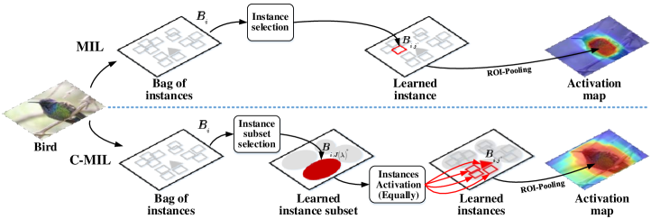
Figure 2: Comparison of the instance selection strategies of MIL and C-MIL. MIL tends to select the most discriminative instance and activate the object part. In contrast, C-MIL selects the most discriminative instance subset. The instances in the subset are activated equally during back-propagation and thus the object extent is activated. (Best viewed in color)

3 Methodology

C-MIL treats images as bags and image regions generated by an object proposal method [32, 24] as instances. The goal is to train instance classifiers (detectors) while solely the bag labels are available. In Fig. 2, $B_{i}\in{\cal B}$ denotes the $i^{th}$ bag (image) and ${\cal B}$ denotes all bags (training images). $y_{i}\in{\cal Y}$ where ${{\cal Y}=\{1,-1\}}$ denotes the label of bag $B_{i}$ indicating the bag contains positive instances ($i.e.$, objects with positive class) or not. $y_{i}=1$ indicates a positive bag (image) that contains at least one positive instance, while $y_{i}=-1$ indicates a negative bag where all instances are negative. Let $B_{i,j}$ and $y_{i,j}$ denote instances and instance labels in bag $B_{i}$, where $j\in\{1,2,...,N\}$ and $N$ the number of instances. $w$ denotes network parameters to be learned.

3.1 MIL Revisit

With above definitions, an MIL method [33, 18, 19] can be separated into two alternative steps: instance selection and detector estimation. In the instance selection step, an instance selector $f(B_{i,j},w_{f})$, which computes the object score of each instance, is used to mine a positive instance (object) from $B_{i}$.

$$B_{i,j^{*}}=\mathop{\arg\max}\nolimits_{{j}}f\left({{B_{i,j}},{w_{f}}}\right),$$ (1)

where $w_{f}$ indicates the parameters of the instance selector and $j^{*}$ the index of the selected instance of the highest score. With selected instances, a detector $g_{z}(B_{ij},w_{g})$ with parameter $w_{g}$ is trained, where $z\in{\cal Y}$. $w_{f}$ and $w_{g}$ respectively denote parameters for the instance selector and detector.

In MIL networks [8, 22, 34], the two alternative steps are integrated and $f(B_{i,j},w_{f})$ and $g_{z}(B_{i,j},w_{g})$ are jointly optimized with loss functions on training images $\cal B$, as

$${\cal F}({\cal B},w)=\sum\nolimits_{i}{{{\cal F}_{f}}\left({{B_{i}},{w_{f}}}\right)+{{\cal F}_{g}}\left({{B_{i}},B_{i,j^{*}},{w_{g}}}\right)},$$ (2)

where the first term, loss of instance selection, is defined as

$${{\cal F}_{f}}\left({{B_{i}},{w_{f}}}\right)=\max({0,1-{y_{i}}\mathop{\max}\nolimits_{j}f\left({{B_{i,j}},{w_{f}}}\right)}),$$ (3)

which is the standard hinge loss. The second term, loss of detector estimation, is defined as

$${{\cal F}_{g}}\left({B_{i},B_{i,j^{*}},{w_{g}}}\right)=-\sum\nolimits_{z}\sum\nolimits_{j}{{\delta_{z,y_{i,j}}}\log g_{z}\left({{B_{i,j}},{w_{g}}}\right)},$$ (4)

where $y_{i,j}$ is defined following the VOC metric [25] as

$${y_{i,j}}=\left\{{\begin{array}[]{*{20}{c}}{+1,if\;IoU\left({{B_{i,j}},B_{i,j^{*}}}\right)\geq 0.5}\\ {-1,if\;IoU\left({{B_{i,j}},B_{i,j^{*}}}\right)<0.5}\end{array}}\right..$$ (5)

$\delta_{a,b}$ is the Kronecker function which is defined as: $\delta_{a,b}=1\;if\;a=b$, and 0 otherwise.

3.2 Convexity Analysis

Recall that the maximum of a set of convex functions is convex. When $y_{i}=-1$, Eq. 3 is convex, but when $y_{i}=1$, it is non-convex. The loss function (Eq. 2) of the MIL network is therefore non-convex as its first term (Eq. 3) is non-convex, and it may have many local minima when provided with bags of numerous instances. Once false positives are mined by the instance selector, the detector will be misled by them, particularly in the early training epochs.

With above analysis, it is concluded that the following two problems remain to be elaborated: 1) How to optimize the non-convex function, and 2) How to perform instance selection in the early training stages when the instance selector is not well trained.

3.3 Continuation MIL

We propose a new optimization method, called Continuation Multiple Instance Learning (C-MIL), and target at solving the above two problems. Instead of introducing regularizers into the loss functions, we directly focus on them from an optimization perspective, by partitioning instances in a bag into subsets and manipulating the non-convexity or smoothness of the loss function defined by Eq. 3.

C-MIL roots in the traditional continuation method  [2], tracing a series of implicitly defined smoothed loss functions from a start point $(w^{0},0)$ to a solution point $(w^{*},1)$, Fig. 1(b), where $w^{0}$ is the solution of ${{\cal F}\left({{\cal B},w,\lambda}\right)}$ when $\lambda=0$, and $w^{*}$ the solution when $\lambda=1$. Accordingly, we define a series of $\lambda$, $0=\lambda_{0}<\lambda_{1}<...<\lambda_{T}=1$, and update Eq. 2 to a continuation loss function, as

$$\small\begin{split}{w^{*}}&=\mathop{\arg\min}\limits_{w}{{\cal F}\left({{\cal B},w,\lambda}\right)}\\ &=\mathop{\arg\min}\limits_{w_{f},w_{g}}\sum\limits_{i}{{{\cal F}_{f}}\left({{B_{i}},{B_{i,J(\lambda)}},{w_{f}}}\right)+{{\cal F}_{g}}\left({{B_{i}},B_{i,J(\lambda)},{w_{g}}}\right)},\end{split}$$ (6)

where ${B_{i,J(\lambda)}}$ denotes the instance subset and $J(\lambda)$ the index of ${B_{i,J(\lambda)}}$, determined by parameter $\lambda$. ${{\cal F}_{f}}\left({{B_{i}},{B_{i,J(\lambda)}},{w_{f}}}\right)$ is the continuation loss function for instance selection, and ${{\cal F}_{g}}\left({{B_{i}},{B_{i,J(\lambda)}},,{w_{g}}}\right)$ continuation loss function for detector estimation.

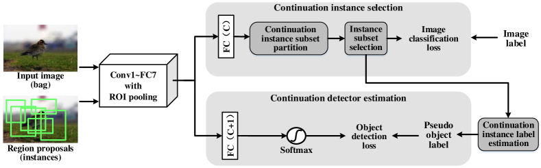
Figure 3: The modules of continuation instance selection and continuation detector estimation are implemented atop a deep network for weakly supervised object detection. $C$ is the number of object categories. In the feed-forward procedure, C-MIL selects positive instances from subsets and uses them as pseudo-objects for detector estimation. In back-propagation, the instance selector and object detectors are jointly optimized with an SGD algorithm.

Continuation instance selection. When learning the instance selector, a bag is partitioned into instance subsets, Fig. 2. In each subset object proposals are spatially related, $i.e.,$ overlapping with each other, and class related, $i.e.,$ having similar object class scores. The subsets are minimum sufficient cover to a bag (image) $B_{i}$, $i.e.,$ $\mathop{\cup}\limits_{J}B_{i,J}={B_{i}}$ and $B_{i,J}\cap B_{i,J^{\prime}}=\emptyset$ for $\forall J\neq J^{\prime}$. All instances in a bag are sorted by their object scores $f\left({{B_{i,j}},{w_{f}}}\right)$ and the following two steps are iteratively performed:

1) Construct an instance subset using the instance of highest object score while not belonging to any other instance subset. 2) Find the instances whose overlap with the highest scored instance $B_{i,j^{*}}$ are larger than or equal to $\lambda$, and then merge them into the subset.

When $\lambda=0$, bag $B_{i}$ is partitioned into a single subset which include all instances. When $\lambda=1$, a bag $B_{i}$ is partitioned into multiple subsets, each of which contains a single instance. The continuation of instance selection is performed from $\lambda=0$ to $\lambda=1$ with the loss function defined as

$$\small{{\cal F}_{f}}\left({{B_{i}},{B_{i,J(\lambda)}},{w_{f}}}\right)=\max({0,1-{y_{i}}\mathop{\max}\limits_{J(\lambda)}f({B_{i,J(\lambda)},{w_{f}}})}),$$ (7)

where $f\left({{B_{i,J(\lambda)}},{w_{f}}}\right)$, the score of instance subset $B_{i,J(\lambda)}$, is defined as

$$f\left({{B_{i,J(\lambda)}},{w_{f}}}\right)=\frac{1}{\left|{B_{i,J(\lambda)}}\right|}\sum\nolimits_{j}{f\left({{B_{i,j}},{w_{f}}}\right)},$$ (8)

where $|{B_{i,J(\lambda)}}|$ denotes the number of instances in subset $B_{i,J(\lambda)}$ and $B_{i,j}\in B_{i,J(\lambda)}$.

During model learning, C-MIL equally utilizes all instances in subset $B_{i,J(\lambda)}$ to fine-tune the network parameters. As the instances are spatially overlapped and class related, C-MIL can collect object/parts for object extent activation, Fig. 2. When $\lambda=0$, each bag $B_{i}$ has a single subset that includes all instances. It is equal to change the term ${\max\nolimits_{j}f\left({{B_{i,j}},{w_{f}}}\right)}$ of Eq. 3 to ${\sum\nolimits_{j}f\left({{B_{i,j}},{w_{f}}}\right)}$ and then Eq. 7 becomes convex. When $\lambda=1$, a bag $B_{i}$ is partitioned into multiple subsets, each of which contains a single instance and thus Eq. 7 deteriorates to the original loss function, Eq. 3. For $0<\lambda<1$, each bag $B_{i}$ has multiple subsets. According to Eq. 8, the score of an instance subset is equal to the average score of instances within that subset. The loss function Eq. 7 is therefore smoother than Eq. 3, and then the loss function of CMIL defined by Eq. 6, is smoother than that of MIL defined by Eq. 2. In other words, a series of smoothed loss functions are defined to alleviate the non-convexity problem of Eq. 3 and discover better solutions [31, 3], Fig. 1(b).

Continuation detector estimation. During model learning, the subset $B_{i,J(\lambda)}$ of highest average score is selected for detector estimation. Considering that there is no bounding box annotation available, the instance selector is inaccurate and the selected subset might contain object parts or backgrounds. We further propose using a continuation strategy to estimate reliable instances and learn detectors.

We propose to partition instances into positives and negatives with the continuation parameter $\lambda$. Denote the learned instance subset as $B_{i,J(\lambda)^{*}}$ and the instance of highest score in $B_{i,J(\lambda)^{*}}$ as $B_{i,j^{*}}$. Instances in the bag are partitioned into positives or negatives according to their spatial relations, as

$${y_{i,j}}=\left\{{\begin{array}[]{*{20}{c}}{+1,if\;IoU\left({{B_{i,j}},B_{i,j^{*}}}\right)\geq 1-\lambda/2}\\ {-1,if\;IoU\left({{B_{i,j}},B_{i,j^{*}}}\right)<\lambda/2}\end{array}},\right.$$ (9)

where $IoU$ calculates the Intersection of Union of two instances (bounding boxes). Eq. 9 defines that instances whose IoU with $B_{i,j^{*}}$ greater than the threshold $1-\lambda/2$ are positives. Instances whose IoU with $B_{i,j^{*}}$ less than $\lambda/2$ are negatives. Instances whose IoU with $B_{i,j^{*}}$ falling into $[\lambda/2,1-\lambda/2]$ are ignored.

During the learning procedure, along with the continuation parameter $\lambda$ changing from 0 to 1, the threshold $1-\lambda/2$ decreases from 1 to 0.5 and the threshold $\lambda/2$ increases from 0 to 0.5. According to Eq. 9, more and more instances are estimated as positives or negatives. Based on these instances, the detector $g_{z}(B_{i,j},w_{g})$ is gradually estimated using the loss function defined as

$${{\cal F}_{g}}\left({B_{i},B_{i,J(\lambda)},{w_{g}}}\right)=-\sum\limits_{z}\sum\limits_{j}{{\delta_{z,y_{ij}}}\log g_{z}\left({{B_{i,j}},{w_{g}}}\right)}.$$ (10)

3.4 Implementation

C-MIL is implemented with an end-to-end deep neural network, with the continuation instance selection and continuation object estimation modules added atop of the FC layers, Fig. 3. In the training phrase, multiple instances, corresponding to region proposals, are first generated for each image using Selective Search method [32]. An ROI-pooling layer atop CONV5 and two fully connected layers are used for instance feature extraction. In the feed-forward procedure, C-MIL selects positive instances from subsets and uses them as pseudo-objects for detector estimation. In back-propagation, the instance selector and object detectors are jointly optimized with an SGD algorithm. With forward- and back-propagation procedures, network parameters are updated and the instance selector and object detectors are learned.

The detection procedure involves instance feature extraction and instance classification Fig. 3. The learned detector computes object scores for all instances and Non-Maximum Suppression (NMS) is used to remove the overlapping instances.

4 Experiments

C-MIL was evaluated on the PASCAL VOC 2007 and PASCAL VOC 2012 datasets using mean average precision (mAP) [25] and correct localization (CorLoc) metrics [36], where Cor-Loc is the percentage of images for which the region of highest score has at least 0.5 interaction-over-union (IoU) with the ground-truth object region. In what follows, we first introduced the experimental settings, then analyzed the effect of the functions defined for the continuation parameter. The Stable Semantic Extremal Regions (SSERs) which appeared during the training procedure of C-MIL were also discussed. Finally, we reported the performance of C-MIL on WSOD and compared it with the state-of-the-art methods.

4.1 Experimental Settings

C-MIL was implemented based on the VGGF and VGG16 CNN model [23] pre-trained on the ILSVRC 2012 dataset [1]. We used Selective Search [32] to extract 2000 object proposals as instances for each image, and removed those whose width or height was less than 20 pixels.

The input images were re-sized into 5 scales {480, 576, 688, 864, 1200} with respect to the larger side (height or width). The scale of a training image was randomly selected and the image was randomly horizontal flipped. In this way, each test image was augmented into a total of 10 images [8, 34, 14]. During learning, we employed the SGD algorithm with momentum 0.9, weight decay 5e-4, and batch size 1. The model iterated 20 epochs where the learning rate was 5e-3 for the first 10 epochs and 5e-4 for the last 10 epochs. During testing, the output scores of each instance from the 10 augmented images were averaged.

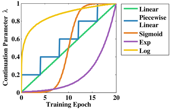
Figure 4: Five functions defined to control the change of continuation parameter.

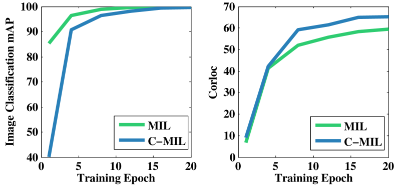
Figure 5: Evolution of image classification and object localization performance during training.

Table 1: Comparison of five functions controlling the change of continuation parameter $\lambda$. Detection and localization performance (%) on the VOC 2007 dataset with VGGF.

Method	Approaches /	mAP	CorLoc
	Continuation Functions
MIL	ContextNet [22]	36.0	55.0
C-MIL (Ours)	Linear	37.9	58.9
	Piecewise Linear	37.6	57.4
	Sigmoid	38.3	58.4
	Exp	37.1	56.4
	Log	40.7	59.5

Table 2: Ablation experimental results of C-MIL. Detection performance (%) on the VOC 2007 dataset with VGGF.

Method	Instance	Object	mAP
	Selector	Detector
MIL [22]	-	-	36.0
C-MIL (Ours)	✓		39.0
		✓	37.4
	✓	✓	40.7

4.2 Continuation Method

In this section, we investigated how to control the continuation parameter $\lambda$ and evaluated the effect on instance selection and detector estimation. All experiments are conducted on VOC 2007 benchmark.

Continuation parameter $\lambda$. To control the change rate of parameter $\lambda$ during training, five functions were evaluated, Fig. 4, and the results are shown in Table 1. With continuation optimization the detection and localization performance respectively improved by 1.1%$\sim$4.7% and 1.4%$\sim$4.5%.

Table 1 shows that the “Log” function reported the best performance. With a “Log” function $\lambda$ increased quickly in the early training epochs while changed slowly in the late epochs, Fig. 4. This is consistent with the learning procedure: in the early training epochs, the instance subsets were large, and it required to dwindle them towards the positive instances; in the later epochs, the instance subsets tended to be stable and it required to focus on detector estimation.

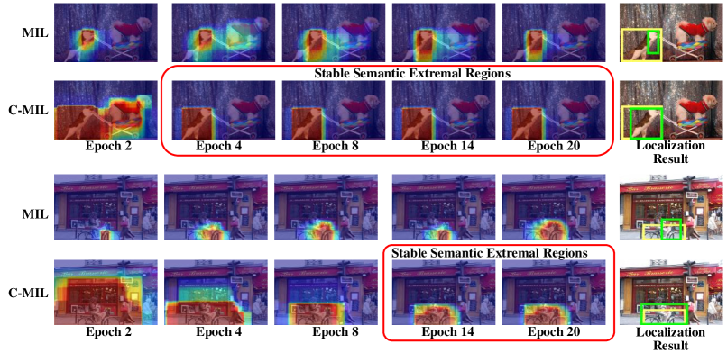
Figure 6: Stable Semantic Extremal Regions (SSERs). MIL activated the discriminative regions for image classification but missed full object extent. C-MIL discovered SSERs indicating full object extent. The continuation parameter $\lambda$ of C-MIL increased from 0 to 1 along with the training procedure from epoch 0 to epoch 20. Yellow boxes and green boxes in the last column denote ground-truths and localization results, respectively. (Best viewed in color)

Continuation optimization. Table 2 shows the ablation experimental results of continuation instance selection and continuation detector estimation. Compared with the baseline approach, introducing the continuation instance selection improved the performance by 3.0% (39.0% vs. 36.0%); introducing the continuation of object estimation further improved the performance by 1.4% (37.4% vs. 36.0%). Combining two modules aggregated the performance 4.7% (40.7% vs. 36.0%), which clearly indicated the effectiveness of continuation optimization designed for C-MIL.

In Fig. 5, we visualized the evolution of the image classification and object localization during training. MIL achieved higher classification performance than C-MIL in the early training epochs. In the later epochs, the classification performance of C-MIL caught up with that of MIL and the localization performance kept higher than that of MIL. The reason lies in that MIL mainly optimized image classification without considering object localization. Therefore, it tended to discover regions which were discriminative for image classification but missed the object location. In contrast, C-MIL optimized both image classification and object localization by learning instance subsets, where object proposals are spatially related and class related.

4.3 Stable Semantic Extremal Regions

To understand the continuation optimization, we visualized the learned subsets/instances in different training epochs in Fig. 6. It can be seen that the instance subsets (activated regions) gradually dwindle with the increase of $\lambda$ from 0 to 1. In the early learning epochs, large subsets were defined to collect object/parts as many as possible. In the later learning epochs, the instance subsets stopped dwindling and tended to form stable activation regions around object boundaries. Such regions, referred to as Stable Semantic Extremal Region (SSERs), often turn out to be full object extent.

The emergence of SSERs indicated that C-MIL continuously suppressed backgrounds while activating object regions during learning. The procedure is somewhat similar to the process of extracting Maximally Stable Extremal Regions (MSERs) [26]. The difference lies in that the MSERs are defined for grey-level stable regions and extracted in an unsupervised manner while SSERs are defined for semantic stable regions and learned in a weakly supervised manner.

Table 3: Detection performance (%) on the VOC 2007 test set. Comparison of C-MIL to the state-of-the-arts.

Network	Method	aero	bike	bird	boat	bottle	bus	car	cat	chair	cow	table	dog	horse	mbike	person	plant	sheep	sofa	train	tv	mAP
VGGF/ AlexNet	PDA [15]	49.7	33.6	30.8	19.9	13.0	40.5	54.3	37.4	14.8	39.8	9.4	28.8	38.1	49.8	14.5	24.0	27.1	12.1	42.3	39.7	31.0
	LCL+Context [11]	48.9	42.3	26.1	11.3	11.9	41.3	40.9	34.7	10.8	34.7	18.8	34.4	35.4	52.7	19.1	17.4	35.9	33.3	34.8	46.5	31.6
	WSDDN [8]	42.9	56.0	32.0	17.6	10.2	61.8	50.2	29.0	3.8	36.2	18.5	31.1	45.8	54.5	10.2	15.4	36.3	45.2	50.1	43.8	34.5
	ContextNet [22]	57.1	52.0	31.5	7.6	11.5	55.0	53.1	34.1	1.7	33.1	49.2	42.0	47.3	56.6	15.3	12.8	24.8	48.9	44.4	47.8	36.3
	WCCN [14]	43.9	57.6	34.9	21.3	14.7	64.7	52.8	34.2	6.5	41.2	20.5	33.8	47.6	56.8	12.7	18.8	39.6	46.9	52.9	45.1	37.3
	OICR [34]	53.1	57.1	32.4	12.3	15.8	58.2	56.7	39.6	0.9	44.8	39.9	31.0	54.0	62.4	4.5	20.6	39.2	38.1	48.9	48.6	37.9
	MELM [37]	56.4	54.7	30.9	21.1	17.3	52.8	60.0	36.1	3.9	47.8	35.5	28.9	30.9	61.0	5.8	22.8	38.8	39.6	42.1	54.8	38.4
	C-MIL (Ours)	54.5	55.5	34.4	20.3	16.7	53.4	59.2	44.6	8.4	46.0	40.2	40.8	47.7	63.2	22.8	23.2	39.4	44.3	53.8	52.3	40.7
VGG16	WSDDN [8]	39.4	50.1	31.5	16.3	12.6	64.5	42.8	42.6	10.1	35.7	24.9	38.2	34.4	55.6	9.4	14.7	30.2	40.7	54.7	46.9	34.8
	PDA [15]	54.5	47.4	41.3	20.8	17.7	51.9	63.5	46.1	21.8	57.1	22.1	34.4	50.5	61.8	16.2	29.9	40.7	15.9	55.3	40.2	39.5
	OICR [34]	58.0	62.4	31.1	19.4	13.0	65.1	62.2	28.4	24.8	44.7	30.6	25.3	37.8	65.5	15.7	24.1	41.7	46.9	64.3	62.6	41.2
	WCCN [14]	49.5	60.6	38.6	29.2	16.2	70.8	56.9	42.5	10.9	44.1	29.9	42.2	47.9	64.1	13.8	23.5	45.9	54.1	60.8	54.5	42.8
	TS2C [38]	59.3	57.5	43.7	27.3	13.5	63.9	61.7	59.9	24.1	46.9	36.7	45.6	39.9	62.6	10.3	23.6	41.7	52.4	58.7	56.6	44.3
	WeakRPN [35]	57.9	70.5	37.8	5.7	21.0	66.1	69.2	59.4	3.4	57.1	57.3	35.2	64.2	68.6	32.8	28.6	50.8	49.5	41.1	30.0	45.3
	MELM [37]	55.6	66.9	34.2	29.1	16.4	68.8	68.1	43.0	25.0	65.6	45.3	53.2	49.6	68.6	2.0	25.4	52.5	56.8	62.1	57.1	47.3
	C-MIL (Ours)	62.5	58.4	49.5	32.1	19.8	70.5	66.1	63.4	20.0	60.5	52.9	53.5	57.4	68.9	8.4	24.6	51.8	58.7	66.7	63.5	50.5
	OICR-Ens. [34]	65.5	67.2	47.2	21.6	22.1	68.0	68.5	35.9	5.7	63.1	49.5	30.3	64.7	66.1	13.0	25.6	50.0	57.1	60.2	59.0	47.0
FRCNN	TS2C [38]	-	-	-	-	-	-	-	-	-	-	-	-	-	-	-	-	-	-	-	-	48.0
Re-train	WeakRPN-Ens. [35]	63.0	69.7	40.8	11.6	27.7	70.5	74.1	58.5	10.0	66.7	60.6	34.7	75.7	70.3	25.7	26.5	55.4	56.4	55.5	54.9	50.4
	C-MIL (Ours)	61.8	60.9	56.2	28.9	18.9	68.2	69.6	71.4	18.5	64.3	57.2	66.9	65.9	65.7	13.8	22.9	54.1	61.9	68.2	66.1	53.1

4.4 Performance

Table 3 shows the performance of C-MIL and a comparison with the state-of-the-art methods on the PASCAL VOC 2007 dataset. It can be seen that C-MIL respectively achieved 40.7% and 50.5% with the VGGF and VGG16 models. With VGGF, C-MIL respectively outperformed the WCCN [14], OICR [34], and MELM [37] by 3.4% (40.7% vs. 37.3%), 2.8% (40.7% vs. 37.9%) and 2.3% (40.7% vs. 38.4%). With VGG16, it respectively outperformed the WeakRPN [35], TS²C [38], and MELM [37] by 6.2% (50.5% vs. 44.3%), 5.2% (50.5% vs. 45.3%), and 3.2% (50.5% vs. 47.3%), which were large margins in terms of the challenging WSOD task.

We further re-trained an Fast-RCNN detector using the learned pseudo objects as ground-truth, and achieved 53.1% mAP, as shown in Table 3, which outperformed the state-of-the-art methods by 2.7%$\sim$6.1%. Specifically, the detection performance for “aeroplane” (+3.2%), “bird” (+5.8%), “cat” (+3.5%), “train” (+4.5%) significantly improved.

Table 4 shows the detection results of the proposed C-MIL and the state-of-the-art methods on the PASCAL VOC 2012 dataset with VGG16. For detection, C-MIL respectively outperformed the WeakRPN [35], TS²C [38], and MELM [37] by 5.9% (46.7% vs. 40.8%), 6.7% (46.7% vs. 40.0%), and 4.3% (46.7% vs. 42.4%).

We evaluated object localization performance of C-MIL and compared it with the state-of-the-art methods in Table 4 and Table 5. The used Correct Localization (CorLoc) metric [36] is the percentage of images for which the region of highest object score has at least 0.5 interaction-over-union (IoU) with the ground-truth. It can be seen that C-MIL respectively outperformed the WeakRPN [35] and TS²C [38] by 1.2% (65.0% vs. 63.8%) and 4.0% (65.0% vs. 61.0%) on VOC 2007, and 3.0% (67.4% vs. 64.4%) and 2.5% (67.4% vs. 64.9%) on VOC 2012.

Table 4: Detection and localization performance (%) on the VOC 2012 dataset using VGG16. Comparison of C-MIL to the state-of-the-arts.

Method	mAP	CorLoc
WCCN [14]	37.9	-
Self-Taught [21]	38.3	58.8
OICR [34]	37.9	62.1
TS2C [38]	40.0	64.4
WeakRPN [35]	40.8	64.9
MELM [37]	42.4	-
C-MIL (Ours)	46.7	67.4

Table 5: Localization performance (%) on the VOC 2007 $trainval$ set. Comparison of C-MIL to the state-of-the-arts.

CNN	Method	mAP
VGG16	WSDDN [8]	53.5
	WCCN [14]	56.7
	OICR [34]	60.6
	TS2C [38]	61.0
	WeakRPN [35]	63.8
	C-MIL (Ours)	65.0

5 Conclusion

We proposed an elegant and effective method, referred to as C-MIL, for weakly supervised object detection. C-MIL targets alleviating the non-convexity problem of multiple instance learning using a series of smoothed loss functions. These functions were defined by introducing a parametric strategy for instance subset partition and evaluating the training loss according to these subsets in a deep learning framework. C-MIL significantly improved performance of weakly supervised object detection and weakly supervised object localization, in striking contrast with state-of-the-art approaches. The underlying reality is that the continuation optimization combined the deep feature learning first collects object/object parts to activate true object extent and then discovers Stable Semantic Extremal Regions (SSERs) for object localization. This provides a fresh insight for the weakly supervised object detection problem.

Acknowledgments. The authors are very grateful to the support by NSFC grant 61836012, 61771447, and 61671427, and Beijing Municipal Science and Technology Commission grant Z181100008918014.

References

- [1] Krizhevsky Alex, Sutskever Ilya, and Hinton Geoffrey E. Imagenet classification with deep convolutional neural networks. In Adv. in Neural Inf. Process. Syst. (NIPS), pages 1097–1105, 2012.
- [2] Eugene L. Allgower and Kurt Georg. Numerical Continuation Methods. 1990.
- [3] Eugene L Allgower, Kurt Georg, and R Hettich. Numerical continuation methods. an introduction. Jahresbericht der Deutschen Mathematiker Vereinigung, 96(1):26–26, 1994.
- [4] Amir Beck and Marc Teboulle. Smoothing and first order methods: A unified framework. SIAM Journal on Optimization, 22(2):557–580, 2012.
- [5] Yoshua Bengio, Jérôme Louradour, Ronan Collobert, and Jason Weston. Curriculum learning. In Proc. 26st Int. Conf. Mach. Learn. (ICML), pages 41–48. ACM, 2009.
- [6] Hakan Bilen, Marco Pedersoli, and Tinne Tuytelaars. Weakly supervised object detection with posterior regularization. In Brit. Mach. Vis. Conf. (BMVC), pages 1997–2005, 2014.
- [7] Hakan Bilen, Marco Pedersoli, and Tinne Tuytelaars. Weakly supervised object detection with convex clustering. In Proc. IEEE Int. Conf. Comput. Vis. Pattern Recognit. (CVPR), pages 1081–1089, 2015.
- [8] Hakan Bilen and Andrea Vedaldi. Weakly supervised deep detection networks. In Proc. IEEE Int. Conf. Comput. Vis. Pattern Recognit. (CVPR), pages 2846–2854, 2016.
- [9] Pratik Chaudhari, Anna Choromanska, Stefano Soatto, Yann LeCun, Carlo Baldassi, Christian Borgs, Jennifer Chayes, Levent Sagun, and Riccardo Zecchina. Entropy-sgd: Biasing gradient descent into wide valleys. In Int. Conf. Learn. Repres., 2017.
- [10] Xiaojun Chen. Smoothing methods for nonsmooth, nonconvex minimization. Mathematical programming, 134(1):71–99, 2012.
- [11] Wang Chong, Huang Kaiqi, Ren Weiqiang, Zhang Junge, and Maybank Steve. Large-scale weakly supervised object localization via latent category learning. IEEE Trans. Image Process., 24(4):1371–1385, 2015.
- [12] Wang Chong, Ren Weiqiang, Huang Kaiqi, and Tan Tieniu. Weakly supervised object localization with latent category learning. In Proc. Europ. Conf. Comput. Vis. (ECCV), pages 431–445, 2014.
- [13] Djork-Arné Clevert, Thomas Unterthiner, and Sepp Hochreiter. Fast and accurate deep network learning by exponential linear units (elus). arXiv preprint arXiv:1511.07289, 2015.
- [14] Ali Diba, Vivek Sharma, Ali Pazandeh, Hamed Pirsiavash, and Luc Van Gool. Weakly supervised cascaded convolutional networks. In Proc. IEEE Int. Conf. Comput. Vis. Pattern Recognit. (CVPR), pages 5131–5139, 2017.
- [15] Li Dong, Huang Jia Bin, Li Yali, Wang Shengjin, and Yang Ming Hsuan. Weakly supervised object localization with progressive domain adaptation. In Proc. IEEE Int. Conf. Comput. Vis. Pattern Recognit. (CVPR), pages 3512–3520, 2016.
- [16] Mingfei Gao, Ang Li, Ruichi Yu, Vlad I Morariu, and Larry S Davis. C-wsl: Count-guided weakly supervised localization. 2018.
- [17] Ross Girshick. Fast r-cnn. In Proc. IEEE Int. Conf. Comput. Vis. Pattern Recognit. (CVPR), pages 1440–1448, 2015.
- [18] Cinbis Ramazan Gokberk, Verbeek Jakob, and Schmid Cordelia. Multi-fold mil training for weakly supervised object lcalization. In Proc. IEEE Int. Conf. Comput. Vis. Pattern Recognit. Workshop, pages 2409–2416, 2014.
- [19] Cinbis Ramazan Gokberk, Verbeek Jakob, and Schmid Cordelia. Weakly supervised object localization with multi-fold multiple instance learning. IEEE Trans. Pattern Anal. Mach. Intell., 39(1):189–203, 2016.
- [20] Caglar Gulcehre, Marcin Moczulski, Francesco Visin, and Yoshua Bengio. Mollifying networks. In Int. Conf. Learn. Repres., 2017.
- [21] Zequn Jie, Yunchao Wei, Xiaojie Jin, Jiashi Feng, and Wei Liu. Deep self-taught learning for weakly supervised object localization. In Proc. IEEE Int. Conf. Comput. Vis. Pattern Recognit. (CVPR), pages 4294–4302, 2017.
- [22] Vadim Kantorov, Maxime Oquab, Minsu Cho, and Ivan Laptev. Contextlocnet: Context-aware deep network models for weakly supervised localization. In Proc. Europ. Conf. Comput. Vis. (ECCV), pages 350–365, 2016.
- [23] Simonyan Karen and Zisserman Andrew. Very deep convolutional networks for large-scale image recognition. In ICLR, 2015.
- [24] Zitnick C. Lawrence and Dollár Piotr. Edge boxes: Locating object proposals from edges. In Proc. Europ. Conf. Comput. Vis. (ECCV), pages 391–405, 2014.
- [25] Everingham Mark, Van Gool Luc, Williams Christopher KI, Winn John, and Zisserman Andrew. The pascal visual object classes (voc) challenge. Int. J. Comput. Vis, 88(2):303–338, 2010.
- [26] Jiri Matas, Ondrej Chum, Martin Urban, and Tomás Pajdla. Robust wide-baseline stereo from maximally stable extremal regions. Image and vision computing, 22(10):761–767, 2004.
- [27] Song Hyun Oh, Lee Yong Jae, Jegelka Stefanie, and Darrell Trevor. Weakly supervised discovery of visual pattern configurations. In Adv. in Neural Inf. Process. Syst. (NIPS), pages 1637–1645, 2014.
- [28] Song Hyun Oh, Girshick Ross, Jegelka Stefanie, Mairal Julien, Harchaoui Zaid, and Darrell Trevor. On learning to localize objects with minimal supervision. In Proc. 31st Int. Conf. Mach. Learn. (ICML), pages 1611–1619, 2014.
- [29] Siva Parthipan and Xiang Tao. Weakly supervised object detector learning with model drift detection. In Proc. IEEE Int. Conf. Comput. Vis. (ICCV), pages 343–350, 2011.
- [30] Shaoqing Ren, Kaiming He, Ross Girshick, and Jian Sun. Faster r-cnn: Towards real-time object detection with region proposal networks. In Adv. in Neural Inf. Process. Syst. (NIPS), pages 91–99, 2015.
- [31] Stephen L Richter and Raymond A Decarlo. Continuation methods: Theory and applications. IEEE Trans. on Sys. Man and Cyber., (4):459–464, 1983.
- [32] Uijlings Jasper RR, Van de Sande Koen EA, Gevers Theo, and Smeulders Arnold WM. Selective search for object recognition. Int. J. Comput. Vis, 104(2):154–171, 2013.
- [33] Andrews Stuart, Tsochantaridis Ioannis, and Hofmann Thomas. Support vector machines for multiple-instance learning. In Adv. in Neural Inf. Process. Syst. (NIPS), pages 561–568, 2002.
- [34] Peng Tang, Xinggang Wang, Xiang Bai, and Wenyu Liu. Multiple instance detection network with online instance classifier refinement. In Proc. IEEE Int. Conf. Comput. Vis. Pattern Recognit. (CVPR), pages 3059–3067, 2017.
- [35] Peng Tang, Xinggang Wang, Angtian Wang, Yongluan Yan, Wenyu Liu, Junzhou Huang, and Alan Yuille. Weakly supervised region proposal network and object detection. In Proc. Europ. Conf. Comput. Vis. (ECCV), pages 352–368, 2018.
- [36] Deselaers Thomas, Alexe Bogdan, and Ferrari Vittorio. Weakly supervised localization and learning with generic knowledge. Int. J. Comput. Vis, 100(3):275–293, 2012.
- [37] Fang Wan, Pengxu Wei, Jianbin Jiao, Zhenjun Han, and Qixiang Ye. Min-entropy latent model for weakly supervised object detection. In Proc. IEEE Int. Conf. Comput. Vis. Pattern Recognit. (CVPR), pages 1297–1306, 2018.
- [38] Yunchao Wei, Zhiqiang Shen, Bowen Cheng, Honghui Shi, Jinjun Xiong, Jiashi Feng, and Thomas Huang. Ts2c:tight box mining with surrounding segmentation context for weakly supervised object detection. In Proc. Europ. Conf. Comput. Vis. (ECCV), pages 434–450, 2018.
- [39] Ren Weiqiang, Huang Kaiqi, Tao Dacheng, and Tan Tieniu. Weakly supervised large scale object localization with multiple instance learning and bag splitting. IEEE Trans. Pattern Anal. Mach. Intell., 38(2):405–416, 2016.
- [40] Qixiang Ye, Tianliang Zhang, Qiang Qiu, Baochang Zhang, Jie Chen, and Guillermo Sapiro. Self-learning scene-specific pedestrian detectors using a progressive latent model. In Proc. IEEE Int. Conf. Comput. Vis. Pattern Recognit. (CVPR), pages 2057–2066, 2017.
- [41] Hao Zheng, Zhanlei Yang, Wenju Liu, Jizhong Liang, and Yanpeng Li. Improving deep neural networks using softplus units. In Proc. IEEE Int. Joint Conf. Neural Networks (IJCNN), pages 1–4, 2015.