The stellar Initial Mass Function of the solar neighbourhood revealed by Gaia

Abstract

I use a sample of more than 120,000 stars in the solar neighbourhood with parallaxes, magnitudes and colours estimated with unprecedented accuracy by the second data release of the Gaia mission to derive the initial mass function of the Galactic disc. A full-forward technique is used to take into account for the population of unresolved binaries, the metallicity distribution, the star formation history and their variation across the Galactic disk as well as all the observational effects. The shape of the initial mass function is well represented by a segmented power-law with two breaks at characteristic masses. It has a maximum at $M\sim 0.15~{}M_{\odot}$ with significant flattening (possibly a depletion) at lower masses and a slope of $\alpha=-1.34\pm 0.07$ in the range $0.25<M/M_{\odot}<1$. Above 1 $M_{\odot}$ the IMF shows an abrupt decline with a slope ranging from $\alpha=-2.68\pm 0.09$ to $\alpha=-2.41\pm 0.11$ depending on the adopted resolution of the star formation history.

1 Introduction

The observational measure of the relative fraction of stars according to their stellar masses $\Psi\equiv dN/dM$ is a long-standing challenge in stellar astrophysics. In particular, the distribution of stellar masses at birth (the so-called "initial mass function"; hereafter IMF) is a key ingredient in all stellar population synthesis and dynamical simulations of galaxies and clusters (Romano, Tosi, & Matteucci, 2006; Lamers, Baumgardt, & Gieles, 2013), it determines the stellar mass-to-light ratio (Courteau et al., 2014) and it has a deep relevance in the understanding of the star formation process (Silk, 1977).

In spite of the extensive effort made by many groups, it is still not clear if the IMF is Universal or whether it depends on some physical parameter (Kroupa, 2001; Bastian, Covey, & Meyer, 2010; Jeřábková et al., 2018, and references therein). Among the various theories of star formation developed so far, two main models provide detailed predictions on the shape and dependence of the IMF on environmental parameters. The first predicts that the IMF is the result of the joint effect of fragmentation and competitive accretion in a clustered environment (Larson, 1978; Bonnell et al., 2001; Hennebelle & Chabrier, 2008). The fragmentation of the molecular cloud has a mass-dependent efficiency which scales with the Jeans mass. The value of this critical mass depends on the mean molecular weight and on the density of the gas in a complex way depending on the relative efficiency of several complex processes such as e.g. cosmic-rays/photoelectric heating, C/O collisional excitation, dust cooling, etc (Larson, 1998; Jappsen et al., 2005; Chabrier, Hennebelle, & Charlot, 2014). This implies a dependence of the IMF on the chemical composition and on the original structure of the cloud. In the second theory, stars self-regulate their masses balancing the accretion rate and feedback (Adams & Fatuzzo, 1996). Because of the existence of complex substructures in molecular clouds, it is not possible to define a single characteristic mass and the shape of the IMF is determined by the superposition of the stochastic distributions of many parameters (sound speed, rotation rate, etc.). Also in this case, both the accretion rate and the stellar feedback have a metallicity dependence because of their effect on the sound speed and on the radiation/matter coupling (Adams & Laughlin, 1996). On the other hand, observational evidence has provided controversial results so far (Zakharova, 1989; Kroupa, 2002; Portinari et al., 2004; Ballero, Kroupa, & Matteucci, 2007; Hoversten & Glazebrook, 2008; van Dokkum & Conroy, 2010; Hennebelle, 2012; Geha et al., 2013; Dib, 2014; El-Badry, Weisz, & Quataert, 2017).

Both stellar and dynamical evolution modify the IMF at its extremes: massive stars evolve faster than low-mass ones, so the present-day mass function (PDMF) contains only those stars born within a time interval shorter than their evolutionary timescales. The PDMF is therefore depleted in high-mass stars with respect to the IMF by an amount that depends on the star formation history (SFH) of the considered stellar system (Schroeder, 1998). On the other hand, in stellar systems where a significant number of long-range interactions occurred, the tendency toward kinetic energy equipartition leads low-mass stars to gain orbital energy more efficiently than massive ones, possibly reaching the critical energy needed to escape (Spitzer, 1940). The characteristic timescale over which a significant exchange of kinetic energy among stars occurs is the half-mass relaxation time ($t_{rh}$). As time passes and $t_{age}>>t_{rh}$, the mass function (MF) is progressively depleted at its low-mass end. So, the MF observed today differs from the IMF.

The most intuitive and straightforward technique to derive the PDMF is based on the conversion of the luminosity (absolute magnitude) distribution of the Main Sequence (MS) stars into masses through the comparison with theoretical isochrones (Limber, 1960). This evolutionary sequence does indeed define a locus where stars of different masses spend the majority of their lives with luminosities mainly depending on their masses (Demarque & Mengel, 1973). From an observational point of view, this task is complicated by many factors introducing significant uncertainties.

First, the derivation of absolute magnitudes implies the knowledge of stellar distances. Distances of stellar systems can be derived with relatively good accuracy using different techniques based on the magnitudes of standard candles such as pulsating variables, binaries and stars at the tip of the Red Giant Branch (Lacy, 1978; Bellazzini, Ferraro, & Pancino, 2001; Sollima, Cacciari, & Valenti, 2006). The situation is however more complex for individual stars in the Galactic field which are displaced across two orders of magnitudes in distance. Until recent years, geometric techniques such as trigonometric parallaxes were effective in measuring distances only until a few tens of pc from the Sun with errors as large as 10% (ESA, 1997). Because the completeness of the observational sample depends on the apparent magnitude, bright/massive stars are over-represented in a magnitude-limited sample and a suitable correction accounting for the spatial distribution of stars with different masses is necessary (Miller & Scalo, 1979).

Furthermore, the color and magnitude of MS stars also depend, beside mass, on chemical composition. Therefore, in stellar systems containing stars with different metallicities (such as the Milky Way and galaxies in general) stars with different masses overlap across the MS. The metallicity distribution and star formation rate (SFR) change with the height above the Galactic disk because of the dependence of the chemical enrichment efficiency on the density, the long term dynamical evolution and the increasing contamination of the thick disc (Wang et al., 2019).

Moreover, unresolved multiple systems are observed with luminosities resulting from the sum of the luminosities of their individual components and therefore have magnitudes brighter than those of single stars. Many low-mass stars are secondary components of binary systems and are therefore hidden (Kroupa, Tout, & Gilmore, 1991).

Finally, the extinction varies across the sky according to the column density of the dust interposed between the observer and the stars, making them appear redder and fainter than they are. Stellar systems at large distances cover a small area in the sky and intersect a constant dust density and are therefore subject to a relatively homogeneous extinction. Instead, stars in the Galactic disc are characterized by a variable extinction depending on their Galactic latitudes and heliocentric distances (Drimmel & Spergel, 2001).

For these reasons, clusters and associations, formed by thousand of stars with similar ages and chemical composition, lying at the same distance and subject to the same extinction, are ideal benchmarks for this purpose. Unfortunately, globular and massive open clusters, the closest clusters for which the MF can be determined down to the hydrogen-burning limit with a good statistics and level of completeness, are always older than their typical half-mass relaxation time. Their PDMFs are therefore not representative of their IMFs (Moraux & Bouvier, 2012; Sollima & Baumgardt, 2017). Young massive clusters (with ages $<100$ Myr and $M>10^{5}~{}M_{\odot}$) are all located in starburst galaxies at distances $>1~{}Mpc$ (Portegies Zwart, McMillan, & Gieles, 2010). Because they are compact and distant, it is possible to resolve only a few bright stars even with the Hubble Space Telescope (HST) (Weisz et al., 2013, and references therein). The measure of the MF in the galaxies of the Local Volume, while requiring a careful treatment of their metallicity distributions, has become feasible in recent years thanks to HST only for the Magellanic Clouds and the closest Ultra faint dwarfs. In these galaxies, it has been possible to sample the MF down to a limiting mass of $\sim 0.4~{}M_{\odot}$ (Gouliermis, Brandner, & Henning, 2006; Kalirai et al., 2013; Gennaro et al., 2018a). Most of the information on the IMF comes from the associations and star forming regions. Studies conducted in the nearby associations suggest an average power-law slope $\alpha\sim-2.3$ (Scalo, 1998; Kroupa, 2001) although notable examples of clusters with flatter (such as the Arches and Quintuplet clusters; $-1.9<\alpha<-1.7$; Shin & Kim, 2016) or steeper (e.g. NGC 6611; $\alpha\sim-3$; Dib, 2014) MFs exist.

The solar neighbourhood is also a privileged site to study the IMF. Indeed, the IMF modification due to collisional effects in the Galactic disc is negligible and thousand of stars are observable in the solar vicinity. On the other hand, the lack of accurate distances limited the analysis to a small sample of nearby stars. In his pioneering work, Salpeter (1955) converted the luminosity function of the sample available at that time into the MF adopting a constant star formation rate and neglecting the density/age/metallicity variation across the disc and the effect of binaries. This work showed that the IMF is well represented by a single power-law $\Psi\propto M^{\alpha}$ with index $\alpha=-2.35$ over the range $0.4<M/M_{\odot}<10$. In a following study, Miller & Scalo (1979) applied the same technique to an updated luminosity function, adopting a correction for the spatial distribution of stars with different spectral types and assuming three simplified SFHs. They found that the IMF is only weakly dependent on the SFH and provided different analytical fitting functions. Their IMF steepens at increasing masses ranging from $\alpha=-1.4$ at $0.1<M/M_{\odot}<1$ to $\alpha=-2.5$ at $1<M/M_{\odot}<10$ and $\alpha=-3.3$ at $M>10~{}M_{\odot}$. In a series of papers (Kroupa, Tout, & Gilmore, 1991, 1993; Kroupa, 1995, 2001, 2002) Kroupa and collaborators refined the analysis simulating the effect of a population of unresolved binaries. By summarizing their IMF determinations in the Galactic disc and in young clusters they defined a broken power-law with index $\alpha=-0.3$ in the substellar regime ($M<0.08~{}M_{\odot}$), $\alpha=-1.3$ at $0.1<M/M_{\odot}<0.5$ and $\alpha=-2.3$ at $M>0.5~{}M_{\odot}$. Chabrier (2001, 2003a) used a volume-limited sample of stars with known parallaxes cleaned from binaries to derive a log-normal IMF which smoothly covers a wide range of slopes from $\alpha\sim-1.1$ at $0.1~{}M_{\odot}$ to $\alpha\sim-2.9$ at $M=10~{}M_{\odot}$. The existence of peaks and breaks in the IMF is relevant in the context of star formation theories since it determines the existence of characteristic masses where the efficiencies of some of the physical processes involved might have threshold effects (Bonnell, Clarke, & Bate, 2006). In spite of the different observational samples and functional representations, all the quoted studies converged in defining an IMF slope close to $\alpha=-2.3$ at $M>1~{}M_{\odot}$ and a flatter slope at low masses. In recent years, several works tried to recover the IMF of the solar neighbourhood using the sample of stars with trigonometric parallaxes provided by the Hipparcos mission (Dawson & Schröder, 2010; Rybizki & Just, 2015) or through a best fit of the colour-magnitude diagram obtained from the Tycho-2 mission with synthetic stellar population models of the Milky Way (Czekaj et al., 2014; Mor et al., 2018). All these studies measured MF slopes which all agree in the sub-solar regime with the previous determinations but are significantly steeper ($\alpha<-2.8$) at larger masses. Unfortunately, all the above mentioned studies suffer from either the relatively small statistics and the large uncertainties of Hipparcos parallaxes or from the uncertainties on the distribution of stars across the disc.

A revolution in the inventory of the solar neighbourhood is provided by the Gaia astrometric mission (Gaia Collaboration et al., 2018). In particular, the 2nd data release of Gaia listed positions, parallaxes and proper motions for $\sim 1.3\times 10^{9}$ stars across the entire sky with accuracies down to $20~{}\mu as$ and magnitudes and colors with mmag accuracies down to relatively faint magnitudes ($G<20.7$).

Recently, Mor et al. (2019) used Gaia DR2 magnitudes and parallaxes to derive the SFH of the solar neighbourhood. As a byproduct, they constrained the IMF using a three-segment power-law with breaks at fixed masses at 0.5 $M_{\odot}$ and 1.53 $M_{\odot}$. Their best fit slopes appear to depend on the functional form of the SFH, with $\alpha$=-1.4 and -2.5 in the mass ranges below/above 0.5 $M_{\odot}$ assuming an exponential SFH, and $\alpha$=-1.3 and -1.9 when leaving the SFH free to vary without a pre-imposed parametric shape. While extremely valuable, this work was not focussed on the MF determination so that the limited flexibility of their MF does not allow to draw conclusions on its detailed shape.

In this paper, I use the Hertzprung-Russel diagram of the solar neihbourhood provided by Gaia to derive the IMF of this portion of the Galactic disc. In Sect. 2 the adopted selection criteria applied to the global Gaia catalog to define the sample of solar neighbourhood stars are presented. The algorithms to determine the IMF in two different mass regimes are described in Sect.s 3 and 4, respectively. The derived IMF is compared with those estimated by previous works and with those measured in other dynamically unrelaxed stellar systems in Sect. 5. Finally, I discuss the obtained results in Sect. 6

2 sample selection

Figure 1: Left panel: fraction of 2MASS (red) and PS1 (black) sources detected in the Gaia catalog as a function of the Gaia $G$ magnitude. The shaded areas indicate the standard deviation of the 180 analysed fields. Right panels: number density of nearby sample (top) and bright sample (bottom) stars in Galactic coordinates. Darker contours indicate regions with increasing density.

The analysis presented here is entirely based on data from the second data release of the Gaia mission (Gaia Collaboration et al., 2018). The Gaia catalog contains magnitudes in the $G$, $G_{BP}$ and $G_{RP}$ bands, parallaxes ($p$) and proper motions ($\mu_{RA}^{*},~{}\mu_{Dec}$) for $\sim 1.3\times 10^{9}$ stars in both hemispheres.

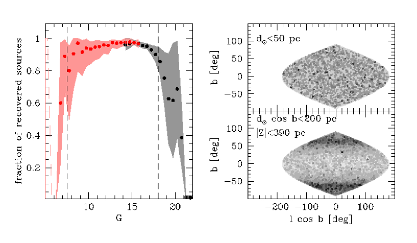
Crucial information for the purpose of this work is the catalog completeness. Stars are included in the Gaia catalog if they are successfully tracked on the focal plane of the Gaia sky mapper in at least five transits and the resulting astrometric solution has an astrometric excess noise and semi-major axis of the position uncertainty ellipse lower than 20 and 100 mas, respectively (Lindegren et al., 2018). According to the Gaia team the catalog is "essentially complete between $12<G<17$" while "a fraction of stars brighter than $G<7$ are missing in the data release" with "an ill-defined faint limiting magnitude" (Arenou et al., 2018). Given the complex Gaia selection function, an estimate of the catalog completeness can be only made through the comparison with other surveys (Marrese et al., 2019). An attempt in this direction was made by Lindegren et al. (2018) who derived the fraction of stars in the OGLE fields (Udalski, Szymanski, Soszynski & Poleski, 2008) sampled by Gaia DR2 to be $\sim$100% at G=18 and $>$95% at G=20 in the Galactic disk. However, as reported in Lindegren et al. (2018), OGLE has a similar limiting magnitude and a poorer spatial resolution than Gaia so that such a comparison provides only an upper limit to the Gaia completeness.

To derive a conservative estimate, I retrieved the positions and magnitudes from the Gaia archive in 180 regions evenly distributed in the sky covering 3 sq. deg. each and cross-correlated them with i) the 2nd data release of the 3$\pi$ Pan-STARRS catalog (PS1; Flewelling, 2018), and ii) the 2Micron All Sky Survey (2MASS; Skrutskie et al., 2006). The PS1 catalog covers 3$\pi$ steradians and is complete down to $g\sim 23.3$ (corresponding to a range in Gaia $G$ magnitude between 21.3 and 23.9 depending on the spectral type) i.e. well below the Gaia limiting magnitude. As most of the catalog samples the Galactic field, crowding is negligible and the limiting magnitude is set by the photon noise. Therefore, this catalog can be considered suitable to estimate the Gaia completeness at faint magnitudes. On the other hand, at magnitudes brighter than $G<14$ the PS1 catalog suffers from photometric saturation, containing many spurious detections surrounding bright stars. In this magnitude range the 2MASS catalog is a valid complement since it is based on shallow infrared photometry and is complete up to very bright magnitudes. To match the three catalogues, stars within $1\arcsec$ were associated and used to construct a colour dependent transformation between the PS1 $g$ and 2MASS K magnitudes into Gaia G magnitudes. Stars with a magnitude difference $\Delta~{}G>0.75~{}mag$ were considered false matches and rejected. The fraction of sources contained in the Gaia catalog as a function of $G$ magnitude is shown in the left panel of Fig. 1. The curves calculated from the comparison with the two reference catalogs nicely match in the interval $14<G<16$. The average fraction of recovered stars is found to be $>90\%$ in the range $7.5<G<18$ with a sudden drop at fainter magnitudes. At bright magnitudes such a fraction shows large variations across the sky with a strong dependence on Galactic latitude. It should be noted that, at low latitudes, most of the incompleteness is caused by the high extinction produced by dust clouds in the Galactic disc, whose density linearly increases with heliocentric distance. This effect is expected to be relatively low in our analysis, which is restricted to the solar neighbourhood. So, the curve shown in Fig. 1 is likely to be a lower limit to the actual completeness of Gaia. On the basis of these considerations, I selected only stars in the range $7.5<G<18$ and do not apply any correction to the derived star counts. Of course, the adoption of magnitude cuts creates a bias in the volume-completeness of stars with different magnitudes, with the faint (bright) stars being under-represented at large (small) distances. This effect must be taken into account in the derivation of the MF (see Sect. 3.1 and 4.1).

I retrieved from the Gaia archive all stars with measured magnitudes and parallaxes and applied a quality cut based on the parameters astrometric_chi2_al ($\chi^{2}$) and astrometric_n_goof_obs_al ($\nu$)

$$\sqrt{\frac{\chi^{2}}{\nu-5}}<1.4~{}u_{0}(G,G_{BP}-G_{RP})$$

Where $u_{0}$ is a function of colour and magnitude (Lindegren et al., 2018). The formal uncertainty on the parallax ($\epsilon_{p}^{\prime}$) was also corrected using the relation

$$\epsilon_{p}=\sqrt{(1.08~{}\epsilon_{p}^{\prime})^{2}+\epsilon_{p,0}^{2}(G)}$$

with

$$\epsilon_{p,0}=\begin{cases}0.021~{}mas&\quad\text{if }G<13\\ 0.043~{}mas&\quad\text{if }G>13\text{~{}~{}\cite[citep]{(\@@bibref{AuthorsPhrase1Year}{2018A&A...616A...2L}{\@@citephrase{, }}{})}}\end{cases}$$

This selection was proven to be effective in removing astrometric artifacts while preserving the completeness of real stars (Arenou et al., 2018).

Gaia is able to resolve binaries with angular separations $>0.4\arcsec$ (Arenou et al., 2018), corresponding to a physical separation $>30~{}AU$ at 50 pc. This means that most of the binaries in our sample are unresolved.

Absolute $M_{G}$ magnitudes were computed according to the relation

$$M_{G}=G-10+5~{}\log{\frac{p}{mas}}-E(B-V)~{}k_{G}$$ (1)

The reddening distribution was assumed to follow the relation

$$E(B-V)=\frac{0.03}{sin~{}b}~{}\left[Erf\left(\frac{p^{-1}sin~{}b_{i}+Z_{\odot}}{\sqrt{2}\sigma_{dust}}\right)-Erf\left(\frac{Z_{\odot}}{\sqrt{2}\sigma_{dust}}\right)\right]$$ (2)

with $\sigma_{dust}=150~{}pc$. Such a relation assumes a gaussian distribution of the dust and has been calibrated using the distance along the reddening vector (from Casagrande & VandenBerg, 2018) in the $(G_{BP}-G)-(G-G_{RP})$ colour-colour diagram of stars in the bright sample as a function of their position in the $p-sin~{}b$ diagram. The above relation, while neglecting small scale variations within the considered volume, well interpolates the reddening map recently obtained by Lallement et al. (2019) ($\Delta E(B-V)=0.003\pm 0.017$).

Different samples were selected to derive the MF in different mass regimes, which require different treatments:

• A sample of nearby ($p>20~{}mas$) MS stars with $M_{G}>4$ to study the MF in the low-mass ($M<1~{}M_{\odot}$) regime (hereafter referred as nearby sample). In this distance range, a star at the hydrogen-burning limit with a solar metallicity (with $M_{G}\sim 15.5$) has an apparent magnitude $G<18$, so this sample contains almost all the low-mass stars contained in this distance range;

• A sample of bright ($M_{G}<4$) stars in a cylinder centred on the Sun with a radius $R\equiv cos(b)/p<200~{}pc$ and height above the Galactic plane $|Z|\equiv|sin(b)/p+Z_{\odot}|<390~{}pc$, to study the MF in the high-mass ($M>1~{}M_{\odot}$) regime (hereafter referred as bright sample).

The R and Z limits of the bright sample were specifically chosen to avoid nearby dust clouds (Lallement et al., 2019). In particular, all the stars within the selected volume nicely lie along the relation defined in eq. 2 reaching a maximum extinction of $E(B-V)<0.035$.

I do not apply any correction for the systematic parallax offset reported by Lindegren et al. (2018). These authors quantify this systematic shift to be $\sim$-0.05 mas at parallaxes $<$2.8 mas and not clearly measurable at large values, with local regional variations depending on colour and magnitude. According to Arenou et al. (2018) "in absence of a large number of calibrators homogeneously spread across the sky in this parallax range, it is not advisable to correct it using a simple shift". Note that, even in the worst case, such an offset would be negligible ($<$2%) in the nearby sample, while it would be partly absorbed by the calibration of the vertical distribution of stars in the bright sample (see Sect. 4).

The value of the solar height above the Galactic plane was set as the mode of the Z distribution of nearby sample stars at $Z_{\odot}=1.4\pm 0.1~{}pc$, which falls between the estimates by Bovy (2017, $-0.9\pm 0.9$ pc) and Karim & Mamajek (2017, $17\pm 5$ pc). Given the vertical extent of our sample, the value of $Z_{\odot}$ is relevant only for the nearby sample. On the other hand, small variations in $Z_{\odot}$ do not produce sizeable effects in the analysis.

To avoid domination by the contribution of individual star clusters located inside the analysed regions, I excluded from the sample the stars belonging to two nearby open clusters (Hyades, Pleiades) and those of two other extended coherent groups not previously identified (at (RA,Dec,p)=(185, -56, 9.2 mas) and (RA,Dec,p)=(-23, 245, 7.3 mas)). These clusters were identified on the basis of their clustering in the 5D space of positions, proper motions and parallax: a star is considered a cluster member if the local density is 3$\sigma$ above the background defined by the stars in the surrounding portion of this space. Consider that, in the generally accepted scenario, the large majority (maybe all) of the field stars form in clusters and associations quickly dissolved after a few Myr. Therefore, regardless of their clustering in phase-space, all the stars of the solar neighbourhood were likely part of a stellar complex at their birth. The selection made here is intended to exclude only the contribution of the largest clusters. Note that these clusters contain only a small fraction of the stars in the considered samples ($\sim$1% of the nearby sample and $<$0.1% of the bright sample), so that the results do not depend on this choice.

After applying the above defined selection criteria, the nearby and the bright samples contain 27048 and 120724 stars, respectively, The number density of the stars belonging to the two samples at various positions in the sky are also shown in the right panels of Fig. 1. Stars nicely follow the expected distribution for the considered sample volumes with no apparent patches, excluding a significant position-dependent sampling efficiency due e.g. to the Gaia scanning law.

In the next two sections I will describe the methods adopted to derive the IMF in the two above defined mass regimes.

3 Low-mass regime

3.1 Method

Figure 2: CMD of the nearby sample. The adopted selection boxes corresponding to the 20 mass-bins (see the text) are shown.

Figure 3: Comparison between the synthetic (bottom-left panel) and observed (bottom-central panel) CMD of the nearby sample. The contributions of single stars (top-left panel) and binaries (top-central panel) to the synthetic CMD are shown separately. The observed (black) and synthetic (red) $G$-band luminosity functions are compared in the bottom-right panel.

The algorithm adopted in this analysis is based on the best fit of the distribution of stars in the $(G_{BP}-G_{RP})-M_{G}$ colour-absolute magnitude diagram (CMD) with a synthetic stellar population.

The masses of $10^{6}$ synthetic particles were extracted from a MF defined in 20 evenly-spaced mass intervals of 0.045 $M_{\odot}$ width, from 0.1 to 1 $M_{\odot}$. The relative fraction of stars in each mass bin ($m_{i}$) is set by 20 coefficients ($k_{i}$)

For a given MF, synthetic absolute magnitudes and colours were derived by interpolating through the set of isochrones of the MESA database (Choi et al., 2016) adopting an age of 10 Gyr. This choice is justified by the fact that the nearby sample is formed by MS stars below the turn-off. In the assumption of a constant star formation rate, 98% of them are older than 200 Myr i.e. the timescale needed by a 0.2 $M_{\odot}$ star to end its pre-MS phase (Tognelli, Prada Moroni, & Degl’Innocenti, 2011). Under these conditions, evolutionary effects are negligible and single-age old isochrones properly reproduce the mass-luminosity relation of these stars.

The metallicity distribution was modelled as an asymmetric gaussian with mode [Fe/H]=0 and a standard deviation of the metal-poor tail $\sigma_{Fe,low}=0.2~{}dex$, while the standard deviation of the metal-rich tail $\sigma_{Fe,hi}$ was left as a free parameter. This model provides the best fit to the colour distribution of the nearby sample and agrees with the metallicity distribution derived by the spectroscopic analysis of 4666 stars in the solar neighbourhood by Mikolaitis et al. (2017).

Synthetic particles were distributed at different heights above the Galactic plane following a gaussian distribution with $\sigma_{Z}=147~{}pc$ and homogeneously along the direction parallel to the Galactic plane over a volume twice larger than that defined for the nearby sample. The value of $\sigma_{Z}$ was chosen as the one maximizing the log-likelihood

$$lnL=-N~{}ln~{}C+\sum_{i=1}^{N}ln~{}P_{i}$$

where

$$P_{i}=\int_{-\infty}^{\infty}exp\left[-\frac{(p-p_{i})^{2}}{2\epsilon_{i}^{2}}-\frac{(p^{-1}sin~{}b_{i}+Z_{\odot})^{2}}{2\sigma_{Z}^{2}}\right]dp$$

$$C=\sqrt{\frac{\pi}{2}}~{}\sigma_{Z}(r_{max}^{2}-Z_{\odot}^{2}-\sigma_{Z}^{2})\times\\ \left[Erf\left(\frac{r_{max}+Z_{\odot}}{\sqrt{2}\sigma_{Z}}\right)+Erf\left(\frac{r_{max-Z_{\odot}}}{\sqrt{2}\sigma_{Z}}\right)\right]+\\ \sigma_{Z}^{2}\left\{(r_{max}-Z_{\odot})~{}exp\left[-\frac{(r_{max}+Z_{\odot})^{2}}{2\sigma_{Z}^{2}}\right]+\right.\\ \left.(r_{max}+Z_{\odot})~{}exp\left[-\frac{(r_{max}-Z_{\odot})^{2}}{2\sigma_{Z}^{2}}\right]\right\}$$

in these equations N is the number of stars in the nearby sample, $b_{i},~{}p_{i}$ and $\epsilon_{i}$ are the Galactic latitude, the parallax and its associated error of the i-th star, $r_{max}=50~{}pc$ and $Z_{\odot}=1.4~{}pc$ (see Sect. 2).

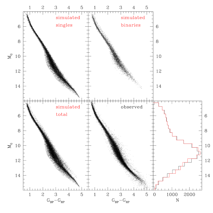
The population of binaries was simulated by random pairing a fraction $f_{b}$ of synthetic stars whose fluxes in the $G$, $G_{BP}$ and $G_{RP}$ passbands were summed.

The dereddened colours and absolute magnitudes of synthetic particles were converted into apparent ones by inverting eq. 1 and a real star with $G$ magnitude within 0.25 mag was associated to each synthetic particle. A gaussian shift in colour, magnitude and parallax with standard deviation equal to the uncertainty of the associated star in the corresponding quantity was then added defining an "observational" set of synthetic apparent magnitudes and parallaxes. Stars with "observational" magnitudes and parallaxes outside the adopted cuts (see Sect. 2) were rejected. The "observational" absolute magnitude of synthetic stars was then re-computed using eq. 1. The above task mimics the effect of photometric and astrometric errors and ensures a proper treatment of the asymmetric distance error (Luri et al., 2018).

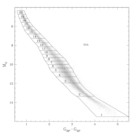
For an assumed binary fraction, an iterative algorithm was used to determine the best fit MF. At the first iteration, guess values of the coefficients $k_{i}\propto m_{i}^{-2.35}$ and of $\sigma_{Fe,hi}=0.2~{}dex$ were adopted. The $(G_{BP}-G_{RP})-M_{G}$ CMD was divided in 20 bins defined to include stars lying in a colour range within 3$\sigma$ about the MS ridge line and at magnitudes corresponding to the mass range of the same 20 bins defining the MF (see above) on a 10 Gyr-old isochrone with solar metallicity. An additional sample of stars with colours redder than 3$\sigma$ with respect to the MS mean ridge line was defined to include unresolved binary systems (see Fig 2). The number of nearby sample stars ($N_{obs,i}$) and synthetic particles ($N_{synth,i}$) contained in each bin were counted and the coefficients $k_{i}$ were updated using the following correction

$$k_{i}^{\prime}=k_{i}\frac{N_{obs,i}\sum_{i}N_{synth;i}}{N_{synth,i}\sum_{i}N_{obs,i}}$$

The value of $\sigma_{Fe,hi}$ was also updated, by increasing (decreasing) its value by 0.005 dex if the fraction of nearby sample stars contained in the binary region was larger (smaller) than that in the synthetic CMD. The above procedure was repeated until convergence, providing for each choice of $f_{b}$ a set of best fit coefficients $k_{i}$. The difference between the distribution of observed and synthetic stars in the CMD was quantified using the penalty function

$$\xi=-\sum_{j}ln~{}\rho_{j}$$ (3)

where $\rho_{j}$ is the density of synthetic particles in the CMD at the position of the j-th nearby sample star

$$\rho_{j}=\left[\left(\frac{(G_{BP}-G_{RP})_{10}-(G_{BP}-G_{RP})_{j}}{\Delta_{BR}}\right)^{2}+\left(\frac{G_{10}-G_{j}}{\Delta_{G}}\right)^{2}\right]^{-1}$$

where $(G_{BP}-G_{RP})_{j},~{}g_{j},~{}(G_{BP}-G_{RP})_{10}$ and $G_{10}$ are the colours and magnitudes of the j-th nearby sample star and of its 10-th nearest neighbour synthetic particle, respectively, and $\Delta_{BR}$ and $\Delta_{G}$ define the metric in the CMD. The best metric is the one maximizing the entropy in the CMD so that $\Delta_{G}/\Delta_{BR}=\sigma_{G}/\sigma_{BR}\sim 2$ where $\sigma_{G}$ and $\sigma_{BR}$ are the standard deviations of magnitude and colour in the nearby sample. The comparison between the CMD and $G$-band luminosity function of the nearby sample and those of the best fit synthetic model is shown in Fig. 3.

Uncertainties were estimated through a Monte Carlo technique: at each step a synthetic CMD containing the same number of stars of the nearby sample was simulated assuming the best fit MF, metallicity distribution and binary fraction and its MF was estimated in the same fashion as for real data. The r.m.s of the MFs of $10^{4}$ different simulations were adopted as the corresponding uncertainties. This procedure takes into account the effect of Poisson noise but does not include the effect of all the systematics (e.g. uncertainties in isochrones, mass-ratio distribution of binaries, spatial distribution, limiting magnitude, etc.).

3.2 Results

Table 1: PDMF of the solar neighbourhood in the sub-solar mass regime. The determinations using two different stellar evolution models are listed. In both cases, the adopted magnitude interval is $7.5<G<$18.

	MESA		PARSEC
$f_{b}$	25%		30%
$\sigma_{Fe,hi}$	0.13		0.14
log $M/M_{\odot}$	log $\psi$	$\epsilon_{log\psi}$	$log\psi$	$\epsilon_{log\psi}$
-0.953	1.03	0.03	1.10	0.01
-0.811	1.22	0.01	1.08	0.02
-0.704	1.08	0.03	1.00	0.02
-0.619	0.86	0.05	0.91	0.03
-0.547	0.79	0.04	0.82	0.05
-0.486	0.62	0.04	0.71	0.03
-0.432	0.50	0.04	0.64	0.06
-0.385	0.42	0.05	0.57	0.06
-0.342	0.36	0.03	0.51	0.06
-0.302	0.26	0.06	0.43	0.06
-0.266	0.32	0.03	0.39	0.07
-0.233	0.26	0.04	0.33	0.06
-0.202	0.23	0.05	0.29	0.07
-0.174	0.25	0.04	0.31	0.05
-0.147	0.15	0.05	0.22	0.05
-0.121	0.08	0.05	0.15	0.06
-0.097	0.13	0.05	0.12	0.07
-0.074	0.08	0.08	0.02	0.05
-0.053	0.18	0.05	0.16	0.10
-0.032	0.08	0.18	0.08	0.11

Figure 4: Left panel: PDMF of the solar neighbourhood in the low-mass regime ($M<1~{}M_{\odot}$) for different assumptions of the binary fraction $f_{b}$. The inset shows the behaviour of the penalty function $\xi$ as a function of $f_{b}$. Right panel: Comparison between the MF derived using different sets of isochrones, quality cuts and limiting $G$ magnitudes. The shaded area indicate the 1$\sigma$ uncertainties. All the MFs are normalized to their values at $1~{}M_{\odot}$.

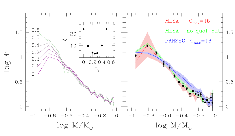
The best fit MFs for different adopted binary fractions and their corresponding values of $\xi$ are shown in the left panel of Fig. 4. It is apparent that the slope of the MF in the mass range $0.25<M/M_{\odot}<1$ is almost independent on the adopted binary fraction, being nicely fit by a single power-law with an index ranging from $\alpha=-1.38$ to -1.16 for $10\%<f_{b}<60\%$, and a best fit value of $\alpha=-1.34\pm 0.07$ at $f_{b}=25\%$. At lower masses the MF significantly flattens and has a peak at $M\sim 0.15~{}M_{\odot}$ although its shape strongly depends on the adopted binary fraction.

The best fit binary fraction ($f_{b}=25\%$) is lower than that measured by the long-baseline spectroscopic campaigns performed in the past ($\sim 50\%$; Duquennoy & Mayor, 1991; Moe & Di Stefano, 2017). Note however that the fraction of binaries estimated here is quite uncertain ($\epsilon_{f_{b}}\sim 10\%$) and refers to unresolved binaries, while some of the wide binaries at small heliocentric distances are resolved by Gaia and therefore included in the nearby sample as single stars. Moreover, the selection on astrometric quality described in Sect. 2 can potentially exclude those binaries for which the relative motion of their components alters the position measured by Gaia, thus worsening the quality of the fit (see below). The corresponding metallicity dispersion on the metal-rich side turns out to be $\sigma_{Fe,hi}=0.13~{}dex$, in agreement with the result by Mikolaitis et al. (2017).

To test the dependence of the measured MF from other assumptions made in the analysis, I repeated the above procedure i) using the isochrones from the PARSEC database (Bressan et al., 2012), ii) assuming a limiting magnitude of $G<15$, and iii) removing the quality cut in the Gaia astrometric solution (see the right panel of Fig.4). The mean slope of the MF does not depend on the adopted isochrones ($\alpha_{PARSEC}=-1.51\pm 0.07$), while some small-scale differences are apparent due to differences in the mass-luminosity relation of these two models. For example, the steepening at $M<0.5~{}M_{\odot}$ apparent when using MESA isochrones is absent in the MF calculated using PARSEC models which are likely spurious. Moreover, with this latter set of models, the MF at $M<0.15~{}M_{\odot}$ is almost flat and does not show any clear peak. It is also possible to fit the MF calculated using the PARSEC isochrones in this mass range with a log-normal function with central value $log~{}(M_{0}/M_{\odot})=1.06$ and $\sigma_{logM}=0.44$, while this analytical representation provides a poor fit at masses $M<0.2~{}M_{\odot}$ when MESA isochrones are used. The MFs in this regime derived using the two sets of models mentioned above are listed in Table 1. No significant differences are noticeable by either changing the adopted limiting magnitude or removing the selection on astrometric quality, indicating that the completeness at $15<G<18$ is still high and that the fraction of artifacts is small and homogeneously distributed in magnitude. It is however worth noting that, when no selection cut on astrometric quality is applied, the best fit is obtained with a fraction of binaries $f_{b}=40\%$, significantly higher than that obtained in the selected sample, indicating that a sizeable fraction of binaries is rejected by the quality cut. This explains the discrepancy between the fraction of binaries estimated here and that of previous literature works.

Since all the stars of the solar neighbourhood in the sub-solar mass regime did not have enough time to evolve off the MS, and because of the non-collisional nature of the Galactic disk, the above derived PDMF is representative of the IMF.

4 High-mass regime

4.1 Method

Figure 5: Left panel: CMD of the bright sample without the upper magnitude cut at $G=7.5$. The selection boxes of the four age bins are marked by black lines. Selected stars are plotted with red ($log~{}t/yr<9$), magenta ($9<log~{}t/yr<9.5$), cyan ($9.5<log~{}t/yr<9.9$) and blue ($9.9<log~{}t/yr<10$) dots. Right panels: histograms of the height above the Galactic plane of the stars belonging to the four age bins. The best fit exponential function is marked by the red line in each panel.

Figure 6: Observed (left panels) and synthetic (middle panels) densities of stars in the CMD of the solar neighbourhood in the absolute magnitude range $4.5<M_{G}<6.5$ in slices at different heights above the Galactic plane. Darker contours delimit regions with higher densities increasing in logarithmic steps of 0.5 dex. The MESA 10 Gyr-old isochrones with metallicities [Fe/H]=-0.5, 0 and +0.5 (from left to right) are overplotted as red lines. The distributions of colour differences about the isochrone at solar metallicity are shown in the right panels for the observed and synthetic CMDs with empty and grey histograms, respectively.

At odds with the portion of CMD fainter than the turn-off point (i.e. less massive than the oldest star which exhausted hydrogen at its centre), the bright part of the CMD is mainly populated by those stars with ages smaller than their evolutionary timescales (see Sect. 1). In this situation the PDMF differs from the IMF which can be estimated only assuming a SFH. This last function can be determined on the basis of the overall distribution of stars in the CMD (Robin, Creze, & Mohan, 1989).

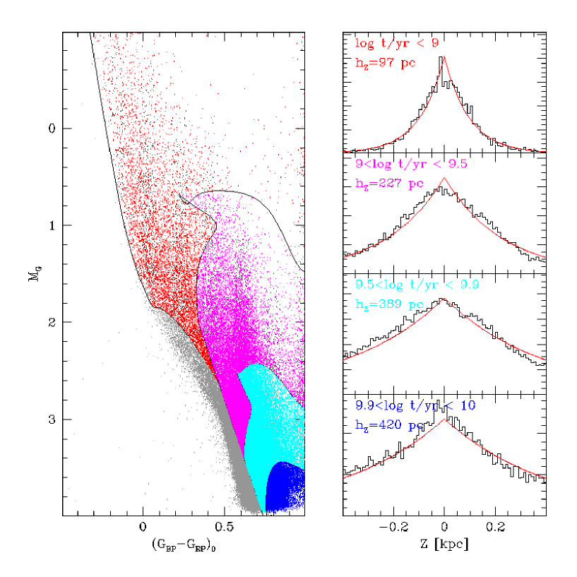
For this purpose I simulated the CMD of the bright sample as the superposition of stellar populations with different ages. The number and width of the age bins determining the resolution of the derived SFH should be chosen as a compromise to ensure flexibility while limiting the degeneracy caused by the increasing number of free parameters. Two cases were considered: i) a low-resolution SFH defined by 4 stellar populations (with ages $log~{}t/yr<9,~{}9<log~{}t/yr<9.5,~{}9.5<log~{}t/yr<9.9$ and $9.9<log~{}t/yr<10$) and ii) a high-resolution SFH defined by 10 stellar populations with ages evenly spaced from 0 to 10 Gyr with a width of 1 Gyr. Within each age bin, star ages were randomly extracted so that they evenly populate the bin. The age upper limit was chosen from the comparison between the lower envelope of the Subgiant Branch observed in the CMD of the bright sample with the MESA isochrone with suitable metallicity (see below).

It is well known that stars at different heights above the Galactic plane have different ages and metallicity distributions. This is a consequence of the dependence of the star formation efficiency on the density, on the secular evolution of the vertical distribution of stars and of the increasing contamination of the thick disc (see Sect. 1). To account for these effects the vertical variations of the age and metallicity distributions were modelled. In particular, the density of stars in each age bin was fitted with an exponential function with scale-height $h_{Z}(t)$. To determine the appropriate scale-height, a synthetic CMD assuming a constant SFR and a Kroupa (2001) IMF was simulated and a selection box in the CMD where the fraction of synthetic particles in the considered age interval is $>90\%$ was defined. The bright sample stars comprised within the appropriate selection box of the dereddened colour-absolute magnitude diagram were used to search the value of $h_{Z}$ which maximizes the log-likelihood

$$lnL=-N~{}ln~{}h_{Z}-N~{}ln\left[1-exp\left(-\frac{Z_{max}}{h_{Z}}\right)\right]+\\ \sum_{i=1}^{N}ln~{}\int_{-\infty}^{\infty}exp\left[-\frac{(p-p_{i})^{2}}{2\epsilon_{i}^{2}}-\frac{|p^{-1}sin~{}b_{i}+Z_{\odot}|}{h_{Z}}\right]dp$$

where $Z_{max}=390~{}pc$ and $Z_{\odot}=1.4~{}pc$ (see Sect. 2). Since the bright magnitude cut at $G=7.5$ removes most of the bright stars at small heliocentric distances altering the overall shape of the distribution, I relaxed this criterion only for this task, thus including all stars brighter than $G<18$. Note that the (possible) incompleteness at bright magnitudes affects only the brightest stars in the youngest age bin at small distances, while the fit is driven by the tails of the distribution. Therefore, this exception is not expected to affect the final result. As expected, the best fit scale-heights for the corresponding age bins increase with age (see Fig. 5). For each age bin, synthetic particles were distributed at different heights above the Galactic plane according to the corresponding distribution and homogeneously along the direction parallel to the Galactic plane over a volume twice larger than that defined for the bright sample.

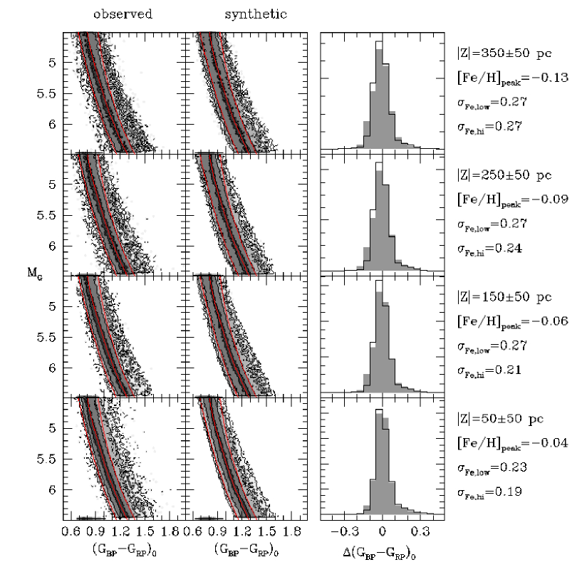
The metallicity distribution at different heights above the Galactic plane was estimated by best-fitting the colour distribution of MS stars ($4.5<M_{G}<6.5$) selected from the Gaia catalog in 4 slices at different heights $\langle|Z|\rangle$ from 50 to 350 pc with a 100 pc width. The absolute magnitudes and dereddened $G_{BP}-G_{RP}$ colours of these stars were calculated using eq.s 1 and 2. A synthetic CMD of that portion of the CMD was simulated using the technique described in Sect. 3.1 and the best fit binary fraction $f_{b}=25\%$ derived in the nearby sample (appropriated for these low-mass stars). In each slice, the metallicity distribution was modelled as an asymmetric gaussian characterized by a mode ($[Fe/H]_{peak}$) and two different standard deviations at the two sides of the distribution ($\sigma_{Fe,low}$ and $\sigma_{Fe,hi}$). The values of these parameters minimizing the penalty function of eq. 3 were chosen as representative of the considered slice. At increasing heights above the Galactic plane, the metallicity distribution appears to shift toward the metal-poor range becoming more symmetric and with increasing dispersions at both sides (see Fig. 6). It is worth noting that the derived metallicity variations are relatively small. This is not surprising since the expected contamination from thick disc stars is small: a comparison with the Robin et al. (2003) model suggests that only 3.3% of the bright sample stars should belong to the thick disc. The metallicity of each star was then extracted by linearly interpolating through the defined distributions according to its height above the Galactic plane. The assumptions made above naturally introduce a height-dependent age-metallicity relation with the particles at larger heights being on average older and more metal-poor than those close to the Galactic plane.

The magnitudes and colours of synthetic stars were derived by interpolating through the set of MESA isochrones of appropriate age and metallicity and assuming a broken power-law IMF with index $\alpha=-1.34$ at $M<1~{}M_{\odot}$ (see Sect. 3.2) and leaving the slope in the high-mass slope as a free parameter. Particles with ages higher than the evolutionary timescales associated to their masses and metallicities were automatically removed from the sample.

A population of binaries was also simulated by adding to the $G,~{}G_{BP}$ and $G_{RP}$ fluxes of a fraction $f_{b}$ of stars those of companion stars with mass extracted from the distribution of mass-ratios described by Moe & Di Stefano (2017) for A-type stars. To limit the number of free parameters, a fixed value of $f_{b}=50\%$ was adopted (Duquennoy & Mayor, 1991). This choice was made to account for the fast changing fraction of multiple systems found by Moe & Di Stefano (2017) in this mass range (50%-90%) and considering that a small fraction of binaries could be actually resolved in the bright sample. The effect of different fractions of binaries is tested in Sect. 4.2.

The effect of reddening, photometric and parallax errors was simulated using the same technique described in Sect. 3.1 and particles satisfying the magnitude and positional cuts adopted for the bright sample (see Sect. 2) are retained.

The relative fractions of stars in the age bins were estimated by matching the $G$-band luminosity function of MS stars at $G_{BP}-G_{RP}<1$ using a least-squares fitting algorithm providing the SFH. Because of the degeneracy between MF slope and SFH, it is always possible to reproduce the luminosity function of MS stars for any choice of the high-mass MF slope. On the other hand, the proportion of old stellar populations is constrained by the relative fraction of evolved stars populating the red portion of the CMD along the Red Giant Branch. The penalty function defined in eq. 3 was calculated using all the stars in the CMD of the bright sample and the value of the high-mass IMF slope providing the lowest value of $\xi$ was derived.

The uncertainty attached to the MF slope was calculated using a Monte Carlo technique (see Sect. 3.1). Although the estimated uncertainty is relatively small, the error budget is dominated by systematics. Indeed, many priors were assumed in the above analysis each of them significantly affecting the final estimate.

Because of the relatively bright cut adopted for our sample ($G>7.5$) massive stars are poorly represented: while the maximum mass in the best fit synthetic catalog is $\sim 10~{}M_{\odot}$, the strongest constraint to the IMF slope is given by stars with $1<M/M_{\odot}<2.5$ which represent more than 96% of the sample. This last interval was considered as the range of validity of the present analysis.

4.2 Results

Table 2: IMF of the solar neighbourhood in the super-solar mass regime. The determinations using two different SFH resolutions are listed. All the determinations are made using MESA isochrones, except the last line where PARSEC isochrones are used.

			low-res SFH		hi-res SFH
		qual.	4 bins		10 bins
$f_{b}$ (%)	$\alpha_{<1~{}M_{\odot}}$	flag	$\alpha$	$\epsilon_{\alpha}$	$\alpha$	$\epsilon_{\alpha}$
30	-2	yes	-2.55	0.08	-2.32	0.10
50	-2	yes	-2.70	0.09	-2.41	0.13
70	-2	yes	-2.74	0.08	-2.46	0.10
50	-2	no	-2.58	0.09	-2.23	0.12
30	-1.34	yes	-2.57	0.06	-2.33	0.10
50	-1.34	yes	-2.68	0.09	-2.41	0.11
70	-1.34	yes	-2.74	0.07	-2.46	0.09
50	-1.34	no	-2.57	0.07	-2.24	0.12
30	-0.5	yes	-2.59	0.07	-2.32	0.11
50	-0.5	yes	-2.67	0.11	-2.42	0.11
70	-0.5	yes	-2.74	0.08	-2.45	0.11
50	-0.5	no	-2.57	0.07	-2.25	0.13
50 (PARSEC)	-1.34	yes	-4.05	0.15	-3.41	0.14

Figure 7: Top panels: comparison between the density in the CMD of the bright sample (top-left) and the prediction of the best fit composite stellar population using 4 (top middle-left) and 10 age components (top middle-right), respectively. Darker contours in the left and central panels delimit regions with higher particle densities increasing by logarithmic steps of 0.5 dex. In the top-right panel the observed and synthetic $G$-band luminosity function of stars bluer than $G_{BR}-G_{RP}<1$ are shown with black, red and blue lines, respectively. Bottom panel: output SFR of the best fit models. The shaded areas indicate the 1$\sigma$ uncertainty.

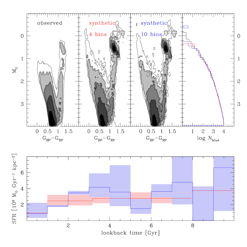
As a result of the procedure described in the previous section, adopting a low-resolution SFH the best fit IMF slope in the super-solar mass regime turns out to be $\alpha=-2.68\pm 0.09$. The best fit model to the bright sample CMD and the $G$-band luminosity function are shown in Fig. 7 together with the derived SFH. The SFH is almost constant over the past 10 Gyr with a slight decrease at recent epochs, in agreement with the results by Bernard (2018) and Mor et al. (2018) within the uncertainties.

A significantly different result is obtained when the high-resolution SFH is adopted. The resulting best fit CMD, $G$-band luminosity function and SFH are also shown in Fig. 7. The corresponding MF turns out to be $\alpha=-2.41\pm 0.11$, significantly flatter than that derived using fewer age components. It can be noticed that, while the general trend of the SFH is compatible with that obtained in the low-resolution case with an increasing star formation rate at old ages, the SFH appears more bursty, being characterized by three intense episodes of star formation which occurred 3, 7 and 10 Gyr ago. However, given the large number of free parameters, it is not clear if such a behaviour is real or rather it is due to the noise or to the degeneracy between the various components.

As reported in Sect. 4.1, beside the effect of the SFH, the results for this mass range strongly depend on the various assumptions. The strongest effect is produced by the adopted isochrones: by repeating the analysis using PARSEC isochrones, the derived IMF slope steepens to $\alpha<-4$. This is a consequence of the different assumptions made by these models on the overshooting in low-mass stars affecting the time spent along the Red Giant Branch and therefore star counts in this evolutive sequence.

The dependence of the derived MF slope as a function of the binary fraction was checked by repeating the analysis assuming different values of $f_{b}$. The high-mass MF slope is found to mildly depends on this assumption varying by $\Delta\alpha=\pm 0.08$ for binary fractions from 30% to 70%. This variation is of the order of the random error so that uncertainties in the prescriptions for the population of binaries are not expected to significantly affect the MF slope in this mass range.

The high-mass MF slope is also found to be independent on the adopted slope at low-masses: by assuming a value in the range $-2<\alpha~{}(M<1~{}M_{\odot})<-0.5$ the derived slope in the high-mass range changes by $\Delta\alpha<0.01$. This is not surprising since the bright sample has been specifically designed to contain only stars at $M_{G}<4$ where only a few low-mass stars in the metal-poor tail of the metallicity distribution are present.

The MF slope was also calculated without applying any selection on the astrometric quality parameter (see Sect. 2). In this case the slope of the MF flattens slightly, remaining however compatible within the errors with that derived for the selected sample.

The entire set of high-mass IMF slopes derived under various assumptions and their associated uncertainties are summarized in Table 2.

5 comparison with previous IMF determinations

5.1 Solar neighbourhood

Figure 8: Comparison between the solar neighbourhood IMF estimated in this work in the sub-solar mass regime (black dots) and the MFs estimated in associations (top-left panel: blue and red dots correspond to the Orion Nebula Cluster and LH95), galaxies (bottom-left panel: blue, red, green, magenta and cyan symbols correspond to the Large and Small Magellanic Cloud, Com Ber, various Ultra faint dwarfs and $\omega$ Cen, respectively) and the most popular parametric fit to the solar neighbourhood (top-right panel: red, blue, green and magenta lines correspond to the works by Salpeter 1955, Kroupa 2001, Chabrier 2003 and Miller & Scalo 1979, respectively; bottom-right panels: red, blue, green, magenta, cyan and yellow lines correspond to the works by Dawson & Schröder 2010, Just & Jahreiß 2010, Czekaj et al. 2014, Rybizki & Just 2015, Mor et al. 2018, 2019, respectively). All the MFs are normalized to their values at $1~{}M_{\odot}$.

Figure 9: Same of Fig. 8 but for the super-solar mass regime. The slope derived in this work using the low-resolution SFH and its 1$\sigma$ uncertainty are represented by the solid line and the grey shaded area, respectively.

In the top-right panels of Fig. 8 and 9 the IMF derived in this work is compared with those provided by Salpeter (1955), Miller & Scalo (1979), Kroupa (2001), and Chabrier (2003b) in the two considered mass regimes, respectively. The IMF estimated here is similar in the sub-solar regime to those of the considered works. Moreover, for the first time, a peak in the IMF at masses above the hydrogen-burning limit is detected. In the super-solar regime a good agreement is found when the high-resolution SFH is adopted, while in the low-resolution case the IMF estimated here is significantly steeper than that found by these authors.

A better agreement with the IMF derived adopting the low-resolution SFH is instead found with the post-Hipparcos IMF determinations (bottom-right panels in Figs. 8 and 9). Dawson & Schröder (2010) estimated a MF slope $\alpha=-2.85\pm 0.15$ from a sample of Hipparcos stars with $M>0.9~{}M_{\odot}$ at heliocentric distances $<$100 pc and within $\pm$25 pc to the Galactic plane. Just & Jahreiß (2010) analysed the data from Hipparcos and the Catalog of Nearby Stars (at distances $<$200 pc) over a mass range $0.5<M/M_{\odot}<10$. They found a broken power-law IMF with indexes $\alpha=-1.46\pm 0.1$ at $M<1.72~{}M_{\odot}$ and $\alpha=-4.16\pm 0.12$ at larger masses. Using the same dataset and a different prescription for the extinction law, Rybizki & Just (2015) updated these values to $\alpha=-1.49\pm 0.08$ at $M<1.39~{}M_{\odot}$ and $\alpha=-3.02\pm 0.06$ beyond this mass. Similar results were obtained by Czekaj et al. (2014) who used the Galactic model by Robin et al. (2003) to derive $\alpha\sim-3$ over a wide range of masses, although their sample is limited at relatively bright magnitudes so that the constraint for stars with masses $M<1.5~{}M_{\odot}$ is less stringent. Mor et al. (2018) performed a similar comparison on the same dataset and found $\alpha=-2.1_{-0.3}^{+0.1}$ in the mass range $0.5<M/M_{\odot}<1.53$ and $\alpha=-2.9\pm 0.2$ at larger masses ($\alpha=-3.7\pm 0.2$ using a different extinction map). Finally, Mor et al. (2019) fitted the Gaia DR2 data with the Besancon model and derived a slope $\alpha=-1.3\pm 0.3$ in the mass range $0.5<M/M_{\odot}<1.53$ and $\alpha=-1.9_{-0.2}^{+0.1}$ at larger masses. However, as in the present analysis, their MF slopes appear to strongly depend on the assumptions about the shape of the SFH: when they impose an exponential SFH, the high-mass slope becomes $\alpha=-2.5\pm 0.1$. At the low-mass extreme ($M<0.5~{}M_{\odot}$) they found positive slopes $\alpha=+0.4_{-0.2}^{+0.6}$ and $\alpha=+0.5_{-0.8}^{+0.5}$ in the case of an exponential or of a non-parametric SFH, respectively. Given the very large uncertainties in this very-low mass range, the difference with respect to our work is not significant.

Considering that all the works quoted above adopt different assumptions for the reddening, the Galactic structure and the adopted stellar models, there is a surprisingly good agreement with the IMF estimated in this work.

5.2 Pleiades

Figure 10: Distribution of stars with parallaxes $p>5~{}mas$ and distance from the Pleiades center $d<7.7^{\circ}$ in the proper motion (top-left panel), parallax (top-right panel), projected position (bottom-left) and colour-magnitude (bottom-right panel) diagrams. Bona-fide members are plotted with red dots. The direction of the bulk proper motion on the X-Y map is shown by an arrow.

Figure 11: Comparison between the Pleiades MF (black dots) and that of the solar neighbourhood (red and blue lines correspond to the low- and high-resolution SFH case, respectively). The shaded area represents the 1$\sigma$ uncertainty. All MFs are normalized to their values at $1~{}M_{\odot}$.

Figure 12: Reconstructed orbit of the Pleiades in the last 130 Myr. The variation of the projected distance on the Galactic plane and of the height above the Galactic plane as a function of the lookback time are shown in the left and right panels, respectively.

As shown in Sect. 4.1, the procedure to derive the IMF in the solar neighbourhood involves many free parameters and suffers from significant systematic errors, in particular in the super-solar mass regime. While this is an unavoidable situation in the Galactic field, a more robust estimate could be made in a nearby stellar system where stars are all located at the same distance and have similar ages and chemical compositions (see Sect. 1). Among the open clusters contained in the volume defined for the bright sample, the Pleiades are young and massive enough to sample a relatively wide range of masses with a good statistics.

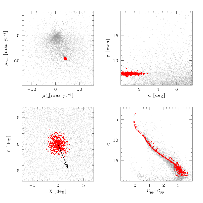
In this cluster, Gaia proper motions and parallaxes allow to select member stars with an unprecedented efficiency on the basis of the distribution of stars in the 5D space formed by projected positions, proper motions and parallaxes. In this space the Pleiades are clustered around a mean proper motion $\langle\mu_{RA}^{*}\rangle=19.96\pm 0.04~{}mas/yr$, $\langle\mu_{Dec}\rangle=-45.51\pm 0.04~{}mas/yr$ and a mean parallax of $\langle p\rangle=7.335\pm 0.003~{}mas$ (corresponding to a distance of $136.34\pm 0.05$ pc in agreement with the interferometric distance estimated by Pan, Shao, & Kulkarni, 2004). The density of stars in this space was calculated using a k-neighbour algorithm with k=10 and normalizing projected distances and velocities to their r.m.s. Cluster members are then defined as those objects lying in a region characterized by a density at 5$\sigma$ above the average background density calculated in a portion of this space surrounding the region occupied by the bulk of cluster members. By using the above selection criterion I selected 674 bona-fide cluster members (see Fig. 10). To quantify the possible residual contamination from Galactic interlopers the same selection criterion was applied to a control field selected at the same Galactic latitude of the Pleiades and displaced by $\sim 13.5^{\circ}$ in longitude: only 1 star passed the above defined criterion indicating a contamination $<0.2\%$. The maximum projected density in the cluster center is $<4\times 10^{-5}~{}arcsec^{-2}$, so crowding effects are negligible. At the distance of the Pleiades, the completeness cuts of Gaia correspond to masses of 0.13 $M_{\odot}$ and 2 $M_{\odot}$ i.e. comparable with those of the Galactic field.

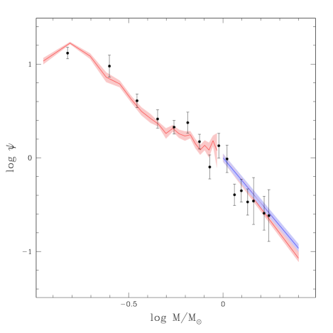
The Pleiades MF was derived in this mass range using the same technique described in Sect. 3.1 assuming a single age ($log~{}t/yr=8.1$) and metallicity ([Fe/H=0]) derived from the comparison with MESA isochrones, in agreement with previous literature determinations (Soderblom et al., 2009; Gossage et al., 2018). Absolute magnitudes were computed from eq. 1 and assuming a reddening of E(B-V)=0.03 (Breger, 1986). Different values of the binary fraction were tested by randomly pairing a fraction of stars extracted from the MF. The best fit MF was chosen as the one providing the lowest value of the penalty function $\xi$ (eq. 3) and it is shown in Fig. 11. It was obtained assuming a binary fraction of $f_{b}=37\%$, smaller than the 76% estimated by Converse & Stahler (2008). The MF derived here is compatible with that estimated by the most comprehensive studies conducted on this stellar system to date (Moraux et al., 2003; Olivares et al., 2018) in the high mass range, although Olivares et al. (2018) derive a significantly flatter MF with $\alpha=-1.12$ in the mass range $0.2<M/M_{\odot}<0.56$.

Qualitatively, the Pleiades MF is remarkably similar to that estimated in the solar neighbourhood over its entire mass extent. In particular, the MF steepens toward high masses with a possible break mass at $M\sim 1~{}M_{\odot}$. A fit with a broken power law gives $\alpha=-1.6\pm 0.2$ and $\alpha=-3.4\pm 0.3$ at masses below/above $1~{}M_{\odot}$. These slopes are slightly steeper but still compatible with those estimated in the Galactic field. In particular, the Pleiades MF slope at masses $M>1~{}M_{\odot}$ is much more similar to that estimated in the solar neighbourhood when a low-resolution SFH is assumed. Part of the difference could be due to the larger binary fraction estimated in this cluster since, as shown in Fig. 4, the binary fraction and the MF slope in the low-mass range are correlated with large binary fractions corresponding to steeper MF slopes. Given the large uncertainty associated to the binary fraction estimate ($\epsilon_{f_{b}}\sim 10\%$), it is possible to obtain a good fit to both the Pleiades and the solar neighbourhood assuming the same binary fraction and MF slope.

The MF of single and binary stars was integrated over the mass range between the hydrogen-burning limit ($0.09~{}M_{\odot}$) and the mass at the tip of the Red Giant Branch ($4.61~{}M_{\odot}$) predicted by the best fit MESA isochrone to estimate the total cluster mass. The contribution to the total mass of white dwarfs was estimated by integrating from the tip of the Red Giant Branch to 8 $M_{\odot}$ and adopting the initial-final mass relation of Kalirai et al. (2008), and is found to be $\sim$1.2%. The estimated total mass of the Pleiades is $365\pm 15~{}M_{\odot}$. The radial cumulative mass distribution of member stars was also calculated and fitted with a King (1966) model with central adimensional parameter $W_{0}=3$ and a half-mass radius of $r_{h}=1.59^{\circ}$ corresponding to 3.8 pc at the distance of the Pleiades. The mass, half-mass radius and number of objects estimated above were used to compute the half-mass relaxation time (Spitzer, 1987) of the Pleiades $t_{rh}=127~{}Myr$. This timescale is comparable to the age of this stellar system so that, while the effect of two-body relaxation could be measurable in massive stars, it could not have significantly altered the global shape of the IMF (Baumgardt & Makino, 2003).

By converting the mean proper motions to projected velocities and adopting a radial velocity of 3.503 km/s (Conrad et al., 2014), I reconstructed the orbit of the Pleiades in the last 130 Myr in a Johnston, Spergel, & Hernquist (1995) potential using a fourth-order Runge-Kutta integrator. The orbit of the Pleiades is confined to a small region of the R-Z plane oscillating between $6.8<R/kpc<8.1$ and reaching a maximum height above the Galactic plane of 70 pc (see Fig. 12).

Summarizing, being dynamically young and having been likely formed in the solar neighbourhood, the Pleiades are a representative episode of recent star formation in the solar vicinity whose IMF has still not been affected by dynamical evolution. The similarity between their MF and that estimated in the field supports the robustness of the IMF derived in Sect. 4.2.

5.3 Comparison with IMF of dynamically unrelaxed stellar systems

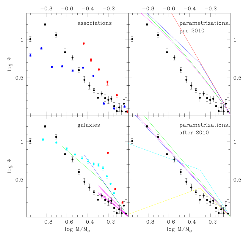
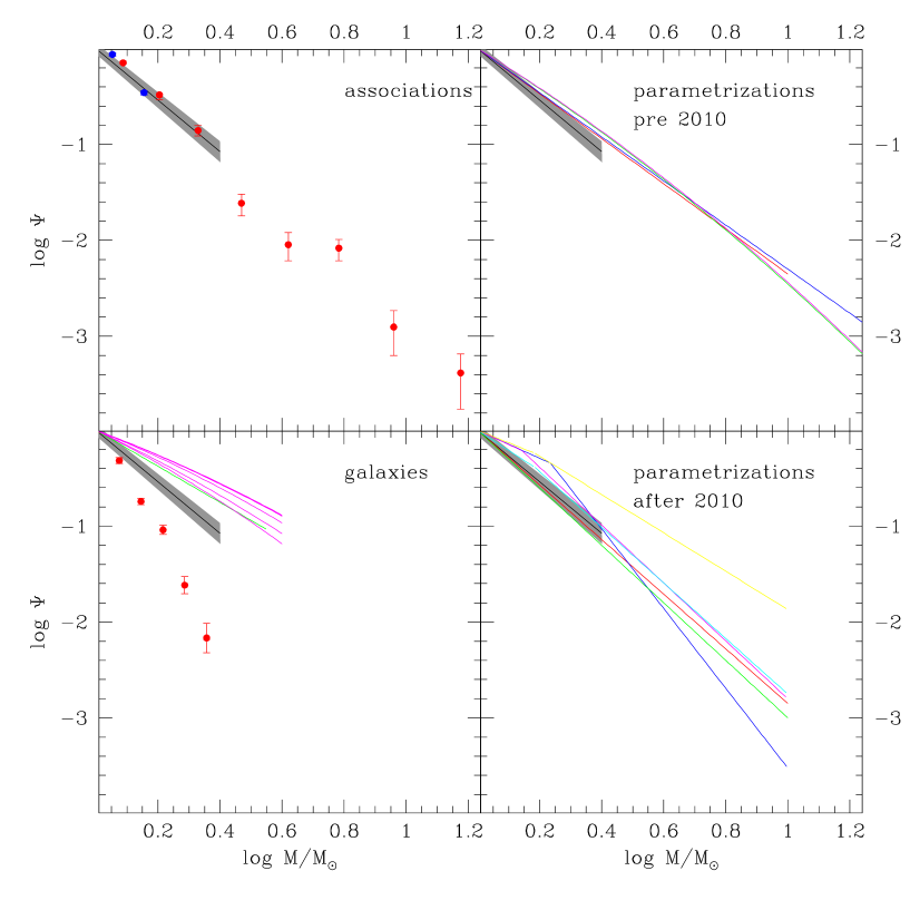
In the left panels of Fig.s 8 and 9, the IMF is compared with those available for a sample of dynamically unrelaxed stellar systems i.e. associations and galaxies. Among nearby associations I considered the deep MF estimates for the Orion Nebula Cluster (with [Fe/H] $\sim$0 and an average age of 2.3 Myr; Da Rio et al., 2012) and the LH95 in the Large Magellanic Cloud ([Fe/H] $\sim$ -0.3, t$\sim$ 4 Myr; Da Rio, Gouliermis, & Henning, 2009). In the sub-solar mass regime the IMF estimated in this work lies between those estimated for these two objects, while at large masses a good agreement is found with the LH95 MF. Note that, according to the quoted errors, at $M<0.4~{}M_{\odot}$ the MFs of these two associations differ significantly. To quantify this difference, a $\chi^{2}$ test was performed selecting the portion of the MFs of these two associations ($log~{}N_{a}$ and $log~{}N_{b}$, respectively) in the n bins in the common mass range. A normalization factor $c$, needed to account for the different mass of the two associations, was calculated as that providing the best match between the two MFs (i.e. the inverse-variance weighted mean of the MF differences in the mass range considered) and applied. The quantity

$$\chi^{2}=\sum_{i=1}^{n}(logN_{a,i}+c-logN_{b,i})/\sqrt{\epsilon_{a,i}^{2}+\epsilon_{b,i}^{2}}$$

was then calculated. If the two estimated MFs are extracted from the same parent distribution, the function above should be distributed as a $\chi^{2}$ with n-1 degrees of freedom. The associated probability ($P_{\chi^{2}}$) is therefore an indicator of the similarity of the two MFs. The above test gives a probability $<10^{-3}$ that the MFs of the two associations are extracted from the same parent distribution. These systems were analysed by the same group with the same technique, so it is unlikely that the difference above can be attributed to systematic errors. Moreover, given their young ages, this difference cannot be interpreted as a result of any dynamical process occurring on such a short timescale and could therefore be primordial.

I also considered the MF measured in a sample of nearby galaxies: the Large and Small Magellanic Clouds (Gouliermis, Brandner, & Henning, 2006; Kalirai et al., 2013), the sample of Ultra faint dwarfs by Gennaro et al. (2018a, b) and $\omega$ Centauri (Sollima, Ferraro, & Bellazzini, 2007), the massive globular cluster with a half-mass relaxation time longer than its age and supposed to be the remnant of an accreted galaxy because of its large metallicity spread (Freeman & Bland-Hawthorn, 2002). The galaxies considered span a wide range in metallicity: from $[Fe/H]\sim-2.7$ for the Ultra-faint dwarfs (Simon et al., 2015) to [Fe/H]=-0.3 for the Large Magellanic Clouds (Luck et al., 1998). Also in this case, at low-masses there is a large spread in the MF measured in these objects. The solar neighbourhood IMF estimated here stands at the lower boundary of the distribution of the considered MFs, being significantly flatter than the steepest ones such as e.g. that of the Small Magellanic Cloud. At masses above the solar mass, for both of the two assumptions on the SFH, the IMF estimated here is comprised between those of the Ultra faint dwarfs and that of the Small Magellanic Clouds. Again, in spite of the large uncertainties involved, there is a wide spread among the various galaxies.

To test the hypothesis that the differences between the MF of these stellar systems and that estimated for the solar neighbourhood are due to random uncertainties, a $\chi^{2}$ test was performed (see above). Significant ($P_{\chi^{2}}<0.3\%$) differences were found with respect to the Orion Nebula Cluster, the Small Magellanic Clouds and $\omega$ Cen, while for the other systems the differences are significant at values $0.3\%<P_{\chi^{2}}<5\%$. The same result is obtained when adopting the solar neighbourhood MF estimated in the low-mass range using the PARSEC isochrones and the MF derived adopting either the low- or the high-resolution SFH in the super-solar regime.

6 summary

I used the most complete and accurate data set available to date provided by the 2nd data release of the Gaia mission to derive the IMF of the solar neighbourhood. The resulting IMF is well represented by a segmented power-law with two breaks at characteristic masses.

The first break occurs in the very low-mass regime where the IMF clearly flattens (and possibly decreases) at $M<0.15~{}M_{\odot}$. This feature does not depend on the adopted stellar models, fraction of binaries or sample completeness. Unfortunately, because of the uncertainties on the mass-luminosity relation at very-low masses, it is not clear whether the deficiency of stars observed at masses below such a break is significant. A similar claim was made by De Marchi & Paresce (1997) on the basis of the analysis of the MF of a sample of Galactic globular clusters. That evidence was however questioned because of the uncertain completeness of their data at faint magnitudes and the possible occurrence of dynamical effects in these old stellar systems (Piotto & Zoccali, 1999).

The existence of a peak in the IMF is predicted by star formation theories although it is not clear if its position should lie in the stellar or sub-stellar regime. It is interesting to analyse the observational evidence presented here in the light of the two main star formation theories. Theories based on the fragmentation on Jeans mass scale + accretion (Larson, 1992; Hennebelle & Chabrier, 2008) predict a peak mass corresponding to the smallest self-gravitating mass in a cloud able to collapse. This characteristic mass depends on the ratio between the thermal Jeans mass and the square of the cloud Mach number (Chabrier, Hennebelle, & Charlot, 2014). These quantities are functions of the thermodynamical properties of the original cloud (temperature, mean molecular weight, density) and on the relative efficiency of those processes affecting turbulent and magnetic pressure. Clouds below this critical mass should not begin star formation unless a local temperature/density/pressure fluctuation causes a decrease of the ratio mentioned above. In this picture, the evidence shown here suggests that in the solar neighbourhood star formation occurred in conditions (low Mach number, low molecular weight, high temperature, small cloud size) favouring the emergence of a peak mass at a relatively high mass. On the other hand, in theories based on the accretion/feedback balance (Adams & Fatuzzo, 1996) the peak in the MF is given by the minimum sound speed (i.e. its thermal value at the cloud temperature) while stars below this mass can still form as a result of fluctuations in the other involved parameters. From their calculation, the IMF peak should lie at $M\sim 0.07M_{\odot}$ slightly lower than the value determined here. Also in this scenario, the existence of a peak in the IMF at $M\sim 0.15M_{\odot}$ suggests conditions leading to a larger minimum sound speed (i.e. larger temperature, lower molecular weight).

In the mass range $0.15<M/M_{\odot}<1$ the MF is well represented by a single power-law with mean slope $\alpha=-1.34\pm 0.07$. This mean value is in agreement within the uncertainties with the average slopes in the same mass range found in all previous works (Miller & Scalo, 1979; Kroupa, 2001; Chabrier, 2003a; Just & Jahreiß, 2010; Rybizki & Just, 2015) although some of these last works adopted different functional forms for the MF. Unfortunately, it is not an easy task to distinguish among the various analytical representations (broken power-law, log-normal, tampered log-normal, etc.) because they almost overlap in this mass range. Moreover, systematic uncertainties in the mass-luminosity relation can create artifacts altering the shape of the MF at small scales (see Sect.3.2). I do not notice any change of slope at $0.5~{}M_{\odot}$ as reported by Kroupa (2001), in agreement with the works by Miller & Scalo (1979), Chabrier (2003a) and Rybizki & Just (2015). While the uncertainties in the mass-luminosity relation described above can hide the evidence of such a break, a significant slope change in this intermediate mass range $0.15<M/M_{\odot}<1$ is not supported by the data analysed here.

At masses larger than 1 $M_{\odot}$, if a smoothly varying SFH is assumed, the average IMF slope is found to be $\alpha=-2.68\pm 0.09$, significantly steeper than those found in works (Salpeter, 1955; Miller & Scalo, 1979; Kroupa, 2001) dated before the most extensive astrometric missions (Hipparcos and Gaia; although a similar value was reported by Kroupa, Tout, & Gilmore, 1993) and compatible with those found in subsequent analyses (Dawson & Schröder, 2010; Just & Jahreiß, 2010; Rybizki & Just, 2015; Mor et al., 2019). Given the improvement in sample size and accuracy of these surveys, these last results seem to be more robust. Unfortunately, this portion of the MF is subject to many systematic uncertainties linked to the modelling of the age/metallicity/distance/reddening variations and on the uncertainties in the SFH (see Sect. 4.2). Indeed, a flatter IMF slope would be compatible with the data if a bursty SFH characterized by rapid variations of the star formation rate were adopted.

A steep IMF is also suggested by the IMF measured in the Pleiades which formed in a single burst of star formation and where no significant spread in metallicity/reddening/distance is expected. The analysis performed in Sect. 5.2 shows that this cluster formed in the solar vicinity and should not have experienced significant dynamical evolution. In the commonly accepted scenario, where the Galactic field population originates in clusters and associations which dissolve in a quick timescale (Kroupa & Weidner, 2003; Kruijssen, 2012; Jeřábková et al., 2018), the IMF measured in the solar neighbourhood is therefore not representative of a single star formation event but is the superposition of contributions of many small episodes. The Pleiades are thus an example in which such building blocks retain the information on the IMF in their PDMF. However, it must be considered that low-mass stars move away from their original site of birth more efficiently than massive ones because of the velocity drift induced by primordial mass segregation and competitive accretion (Bonnell et al., 1997; McMillan, Vesperini, & Portegies Zwart, 2007) and because of their long lifetime, have more time to distribute over the Galactic plane. Therefore, samples of stars covering a wide portion of the field contain preferentially low-mass stars while high-mass ones are confined in more compact portions of the phase-space close to the position of their original birth sites. This effect is responsible for a large cosmic variance in the Galactic disk IMF, with a bias toward measuring steeper IMF slope in the field (Parravano, Hollenbach, & McKee, 2018).

The slopes of the IMF at intermediate and high-masses have been interpreted in different ways by different star formation theories. According to theories of accretion onto Jeans mass scale fragments, accretion occurs in a competitive way at different characteristic stellar radii in different cluster regions according to the relative contribution to the overall cluster potential of gas and stars. In this model, high-mass stars preferentially form in a clustered environment in the central region of the proto-clusters and accrete the majority of their mass at the Bondi-Hoyle radius. The strong mass dependence of the accretion rate results in a steeper IMF with respect to that predicted by simple tidal accretion onto individual fragments typical of low-mass stars. The transition between the accretion- and fragmentation-dominated regimes depends on the prescriptions adopted for primordial mass segregation and on the relative distribution of gas and stars at early stages. In the two regimes considered above the IMF should be characterized by an asymptotic slope $\alpha\sim-1.5$ at low-masses and $\alpha\sim-2.5$ at high-masses (Bonnell et al., 2001). These values are in agreement with those found in the present analysis. In this picture, the results presented here support a transition mass close to 1 $M_{\odot}$ dividing the mass spectrum in two ranges characterized by different slopes. Alternatively, in the Adams & Fatuzzo (1996) theory, the change of IMF slope is due to the different mass-luminosity relation of young stellar objects as a function of their mass (Adams & Fatuzzo, 1996). Indeed, while the luminosity of low mass objects is determined by the infall rate, massive ones generate a significant fraction of luminosity through gravitational contraction, deuterium- and eventually hydrogen-burning. In this case, the transition is extremely smooth and should occur at $\sim 3.1M_{\odot}$. Note that in this simplified model, even assuming a dependence of the IMF slope on the sound speed distribution alone (i.e. the parameter with the largest contribution to the final stellar mass), the IMF slope should have a small variation $-2.1<\alpha<-1.7$ across the entire mass range, much smaller than that observed in this analysis. The stochastic variation of the other parameters involved smoothes the overall IMF further, reducing the slope variation and enhancing the tension with observations. However, the models above contain many simplified recipes to model the complex set of physical processes at work in star forming regions so that it is hard to rule out this scenario on the basis of relatively small differences in the shape of the IMF.

The comparison of the IMF measured in the solar neighbourhood with those estimated in other non-collisional environments (galaxies and associations) reveals a significant degree of variability incompatible with the quoted uncertainties. This would imply that the IMF is not Universal. However, there is no clear trend of the IMF slope with either metallicity or environment. Consider that, as shown in Sect. 4.2, systematic effects can alter the MF slope by a large amount. Since the MFs considered have been estimated by different groups adopting different prescriptions, it is possible that any existing trend could have been erased by such systematic errors.

The analysis presented here will further benefit from the next Gaia data releases. Indeed, besides the incremental improvement of the photometric and astrometric performances, the completeness at bright magnitudes should be established allowing the use of the brightest portion of the luminosity function to constrain the IMF at its high-mass end ($M>2.5~{}M_{\odot}$) and to constrain the SFH at recent epochs with better resolution. Moreover, starting from DR3 metallicities, reddening and a classification of binaries will be provided, thus allowing to calibrate the model parameters better, accounting for their variation across the disc and to replace the statistical population synthesis approach with a star-by-star modelling.

References

- Adams & Fatuzzo (1996) Adams F. C., Fatuzzo M., 1996, ApJ, 464, 256
- Adams & Laughlin (1996) Adams F. C., Laughlin G., 1996, ApJ, 468, 586
- Arenou et al. (2018) Arenou F., et al., 2018, A&A, 616, A17
- Ballero, Kroupa, & Matteucci (2007) Ballero S. K., Kroupa P., Matteucci F., 2007, A&A, 467, 117
- Bastian, Covey, & Meyer (2010) Bastian N., Covey K. R., Meyer M. R., 2010, ARA&A, 48, 339
- Baumgardt & Makino (2003) Baumgardt H., Makino J., 2003, MNRAS, 340, 227
- Bernard (2018) Bernard E. J., 2018, IAUS, 330, 148
- Bellazzini, Ferraro, & Pancino (2001) Bellazzini M., Ferraro F. R., Pancino E., 2001, ApJ, 556, 635
- Bonnell et al. (1997) Bonnell I. A., Bate M. R., Clarke C. J., Pringle J. E., 1997, MNRAS, 285, 201
- Bonnell et al. (2001) Bonnell I. A., Clarke C. J., Bate M. R., Pringle J. E., 2001, MNRAS, 324, 573
- Bonnell, Clarke, & Bate (2006) Bonnell I. A., Clarke C. J., Bate M. R., 2006, MNRAS, 368, 1296
- Bovy (2017) Bovy J., 2017, MNRAS, 470, 1360
- Breger (1986) Breger M., 1986, ApJ, 309, 311
- Bressan et al. (2012) Bressan A., Marigo P., Girardi L., Salasnich B., Dal Cero C., Rubele S., Nanni A., 2012, MNRAS, 427, 127
- Casagrande & VandenBerg (2018) Casagrande L., VandenBerg D. A., 2018, MNRAS, 479, L102
- Chabrier (2001) Chabrier G., 2001, ApJ, 554, 1274
- Chabrier (2003a) Chabrier G., 2003a, ApJ, 586, L133
- Chabrier (2003b) Chabrier G., 2003b, PASP, 115, 763
- Chabrier, Hennebelle, & Charlot (2014) Chabrier G., Hennebelle P., Charlot S., 2014, ApJ, 796, 75
- Choi et al. (2016) Choi J., Dotter A., Conroy C., Cantiello M., Paxton B., Johnson B. D., 2016, ApJ, 823, 102
- Conrad et al. (2014) Conrad C., et al., 2014, A&A, 562, A54
- Converse & Stahler (2008) Converse J. M., Stahler S. W., 2008, ApJ, 678, 431
- Courteau et al. (2014) Courteau S., et al., 2014, RvMP, 86, 47
- Czekaj et al. (2014) Czekaj M. A., Robin A. C., Figueras F., Luri X., Haywood M., 2014, A&A, 564, A102
- Da Rio, Gouliermis, & Henning (2009) Da Rio N., Gouliermis D. A., Henning T., 2009, ApJ, 696, 528
- Da Rio et al. (2012) Da Rio N., Robberto M., Hillenbrand L. A., Henning T., Stassun K. G., 2012, ApJ, 748, 14
- Dawson & Schröder (2010) Dawson S. A., Schröder K.-P., 2010, MNRAS, 404, 917
- De Marchi & Paresce (1997) De Marchi G., Paresce F., 1997, ApJ, 476, L19
- Demarque & Mengel (1973) Demarque P., Mengel J. G., 1973, A&A, 22, 121
- Dib (2014) Dib S., 2014, MNRAS, 444, 1957
- Drimmel & Spergel (2001) Drimmel R., Spergel D. N., 2001, ApJ, 556, 181
- Duquennoy & Mayor (1991) Duquennoy A., Mayor M., 1991, A&A, 248, 485
- El-Badry, Weisz, & Quataert (2017) El-Badry K., Weisz D. R., Quataert E., 2017, MNRAS, 468, 319
- ESA (1997) ESA, 1997, ESASP, 1200,
- Flewelling (2018) Flewelling H., 2018, AAS, 231, 436.01
- Freeman & Bland-Hawthorn (2002) Freeman K., Bland-Hawthorn J., 2002, ARA&A, 40, 487
- Gaia Collaboration et al. (2018) Gaia Collaboration, et al., 2018, A&A, 616, A1
- Geha et al. (2013) Geha M., et al., 2013, ApJ, 771, 29
- Gennaro et al. (2018a) Gennaro M., et al., 2018a, ApJ, 855, 20
- Gennaro et al. (2018b) Gennaro M., et al., 2018b, ApJ, 863, 38
- Gossage et al. (2018) Gossage S., Conroy C., Dotter A., Choi J., Rosenfield P., Cargile P., Dolphin A., 2018, ApJ, 863, 67
- Gouliermis, Brandner, & Henning (2006) Gouliermis D., Brandner W., Henning T., 2006, ApJ, 641, 838
- Hennebelle (2012) Hennebelle P., 2012, A&A, 545, A147
- Hennebelle & Chabrier (2008) Hennebelle P., Chabrier G., 2008, ApJ, 684, 395
- Hoversten & Glazebrook (2008) Hoversten E. A., Glazebrook K., 2008, ApJ, 675, 163
- Jappsen et al. (2005) Jappsen A.-K., Klessen R. S., Larson R. B., Li Y., Mac Low M.-M., 2005, A&A, 435, 611
- Jeřábková et al. (2018) Jeřábková T., Hasani Zonoozi A., Kroupa P., Beccari G., Yan Z., Vazdekis A., Zhang Z.-Y., 2018, A&A, 620, A39
- Johnston, Spergel, & Hernquist (1995) Johnston K. V., Spergel D. N., Hernquist L., 1995, ApJ, 451, 598
- Just & Jahreiß (2010) Just A., Jahreiß H., 2010, MNRAS, 402, 461
- Kalirai et al. (2008) Kalirai J. S., Hansen B. M. S., Kelson D. D., Reitzel D. B., Rich R. M., Richer H. B., 2008, ApJ, 676, 594
- Kalirai et al. (2013) Kalirai J. S., et al., 2013, ApJ, 763, 110
- Karim & Mamajek (2017) Karim M. T., Mamajek E. E., 2017, MNRAS, 465, 472
- King (1966) King I. R., 1966, AJ, 71, 64
- Kroupa (1995) Kroupa P., 1995, ApJ, 453,
- Kroupa (2001) Kroupa P., 2001, MNRAS, 322, 231
- Kroupa (2002) Kroupa P., 2002, Sci, 295, 82
- Kroupa & Weidner (2003) Kroupa P., Weidner C., 2003, ApJ, 598, 1076
- Kroupa, Tout, & Gilmore (1991) Kroupa P., Tout C. A., Gilmore G., 1991, MNRAS, 251, 293
- Kroupa, Tout, & Gilmore (1993) Kroupa P., Tout C. A., Gilmore G., 1993, MNRAS, 262, 545
- Kruijssen (2012) Kruijssen J. M. D., 2012, MNRAS, 426, 3008
- Lacy (1978) Lacy C. H., 1978, ApJ, 226, 138
- Lallement et al. (2019) Lallement R., et al., 2019, A&A, 625, A135
- Lamers, Baumgardt, & Gieles (2013) Lamers H. J. G. L. M., Baumgardt H., Gieles M., 2013, MNRAS, 433, 1378
- Larson (1978) Larson R. B., 1978, MNRAS, 184, 69
- Larson (1992) Larson R. B., 1992, MNRAS, 256, 641
- Larson (1998) Larson R. B., 1998, MNRAS, 301, 569
- Limber (1960) Limber D. N., 1960, ApJ, 131, 168
- Lindegren et al. (2018) Lindegren L., et al., 2018, A&A, 616, A2
- Luck et al. (1998) Luck R. E., Moffett T. J., Barnes T. G., III, Gieren W. P., 1998, AJ, 115, 605
- Luri et al. (2018) Luri X., et al., 2018, A&A, 616, A9
- Marrese et al. (2019) Marrese P. M., Marinoni S., Fabrizio M., Altavilla G., 2019, A&A, 621, A144
- McMillan, Vesperini, & Portegies Zwart (2007) McMillan S. L. W., Vesperini E., Portegies Zwart S. F., 2007, ApJ, 655, L45
- Mikolaitis et al. (2017) Mikolaitis Š., de Laverny P., Recio-Blanco A., Hill V., Worley C. C., de Pascale M., 2017, A&A, 600, A22
- Miller & Scalo (1979) Miller G. E., Scalo J. M., 1979, ApJS, 41, 513
- Moe & Di Stefano (2017) Moe M., Di Stefano R., 2017, ApJS, 230, 15
- Mor et al. (2018) Mor R., Robin A. C., Figueras F., Antoja T., 2018, A&A, 620, A79
- Mor et al. (2019) Mor R., Robin A. C., Figueras F., Roca-Fàbrega S., Luri X., 2019, A&A, 624, L1
- Moraux et al. (2003) Moraux E., Bouvier J., Stauffer J. R., Cuillandre J.-C., 2003, A&A, 400, 891
- Moraux & Bouvier (2012) Moraux E., Bouvier J., 2012, ASSP, 29, 115
- Olivares et al. (2018) Olivares J., et al., 2018, A&A, 617, A15
- Pan, Shao, & Kulkarni (2004) Pan X., Shao M., Kulkarni S. R., 2004, Natur, 427, 326
- Parravano, Hollenbach, & McKee (2018) Parravano A., Hollenbach D., McKee C. F., 2018, MNRAS, 480, 2449
- Piotto & Zoccali (1999) Piotto G., Zoccali M., 1999, A&A, 345, 485
- Portegies Zwart, McMillan, & Gieles (2010) Portegies Zwart S. F., McMillan S. L. W., Gieles M., 2010, ARA&A, 48, 431
- Portinari et al. (2004) Portinari L., Moretti A., Chiosi C., Sommer-Larsen J., 2004, ApJ, 604, 579
- Robin, Creze, & Mohan (1989) Robin A. C., Creze M., Mohan V., 1989, Ap&SS, 156, 9
- Robin et al. (2003) Robin A. C., Reylé C., Derrière S., Picaud S., 2003, A&A, 409, 523
- Romano, Tosi, & Matteucci (2006) Romano D., Tosi M., Matteucci F., 2006, MNRAS, 365, 759
- Rybizki & Just (2015) Rybizki J., Just A., 2015, MNRAS, 447, 3880
- Salpeter (1955) Salpeter E. E., 1955, ApJ, 121, 161
- Scalo (1998) Scalo J., 1998, ASPC, 142, 201
- Schroeder (1998) Schroeder K.-P., 1998, A&A, 334, 901
- Shin & Kim (2016) Shin J., Kim S. S., 2016, MNRAS, 460, 1854
- Silk (1977) Silk J., 1977, ApJ, 214, 718
- Simon et al. (2015) Simon J. D., et al., 2015, ApJ, 808, 95
- Skrutskie et al. (2006) Skrutskie M. F., et al., 2006, AJ, 131, 1163
- Soderblom et al. (2009) Soderblom D. R., Laskar T., Valenti J. A., Stauffer J. R., Rebull L. M., 2009, AJ, 138, 1292
- Sollima & Baumgardt (2017) Sollima A., Baumgardt H., 2017, MNRAS, 471, 3668
- Sollima, Cacciari, & Valenti (2006) Sollima A., Cacciari C., Valenti E., 2006, MNRAS, 372, 1675
- Sollima, Ferraro, & Bellazzini (2007) Sollima A., Ferraro F. R., Bellazzini M., 2007, MNRAS, 381, 1575
- Spitzer (1940) Spitzer L., Jr., 1940, MNRAS, 100, 396
- Spitzer (1987) Spitzer L., 1987, in "Dynamical evolution of globular clusters", Princeton, NJ, Princeton University Press
- Tognelli, Prada Moroni, & Degl’Innocenti (2011) Tognelli E., Prada Moroni P. G., Degl’Innocenti S., 2011, A&A, 533, A109
- Udalski, Szymanski, Soszynski & Poleski (2008) Udalski A., Szymanski M. K., Soszynski I., Poleski R., 2008, AcA, 58, 69
- van Dokkum & Conroy (2010) van Dokkum P. G., Conroy C., 2010, Natur, 468, 940
- Wang et al. (2019) Wang C., et al., 2019, MNRAS, 482, 2189
- Weisz et al. (2013) Weisz D. R., et al., 2013, ApJ, 762, 123
- Zakharova (1989) Zakharova P. E., 1989, AN, 310, 127