Final results for the neutron $\beta$-asymmetry parameter $A_{0}$ from the
UCNA experiment

Abstract

The UCNA experiment was designed to measure the neutron $\beta$-asymmetry parameter $A_{0}$ using polarized ultracold neutrons (UCN). UCN produced via downscattering in solid deuterium were polarized via transport through a 7 T magnetic field, and then directed to a 1 T solenoidal electron spectrometer, where the decay electrons were detected in electron detector packages located on the two ends of the spectrometer. A value for $A_{0}$ was then extracted from the asymmetry in the numbers of counts in the two detector packages. We summarize all of the results from the UCNA experiment, obtained during run periods in 2007, 2008–2009, 2010, and 2011–2013, which ultimately culminated in a 0.67% precision result for $A_{0}$.

1 Introduction

Precision measurements of neutron $\beta$-decay observables, together with precise Standard Model calculations, constitute a sensitive test for new physics gonzalez-alonso-ppns . The UCNA experiment pattie09 ; liu10 ; plaster12 ; mendenhall13 ; brown18 determined the neutron $\beta$-asymmetry parameter $A$, the angular correlation between the neutron’s spin and the decay electron’s momentum, which appears in the angular distribution of the emitted electrons as jackson57

$$d\Gamma(E_{e},\theta)\propto 1+PA\beta\cos\theta.$$ (1)

Here, $E_{e}$ denotes the electron’s energy, $\beta=v/c$ where $v$ is the electron’s velocity, $P$ is the neutron polarization, and $\theta$ is the angle between the neutron’s spin and the electron’s momentum. At lowest order, measurements of $A$ determine the ratio of the weak axial-vector and vector coupling constants, $\lambda\equiv g_{A}/g_{V}$, according to jackson57

$$A_{0}=-2\frac{\lambda^{2}-|\lambda|}{1+3\lambda^{2}}.$$ (2)

The UCNA experiment was carried out at the Ultracold Neutron Facility at the Los Alamos Neutron Science Center saunders13 ; ito18 , and was the first-ever measurement of any neutron $\beta$-decay angular correlation parameter using Ultracold Neutrons (UCN). UCNA has provided for the determination of $A$ via a complementary technique to cold neutron beam-based measurements of $A$, such as from the PERKEO III experiment saul-ppns ; markisch18 , via the use of different techniques for the neutron polarization, different sensitivity to environmental and neutron-generated backgrounds, and different methods for electron detection, among others.

2 Overview of the UCNA Experiment

An overview of the basic operating principles of the UCNA experiment plaster12 is as follows, of which a schematic diagram is shown in Fig. 1. A pulsed 800 MeV proton beam, with a time-averaged current of 10 $\mu$A, was incident on a tungsten spallation target. The emerging neutrons were moderated in cold polyethylene, then downscattered to the ultracold regime in a crystal of solid deuterium. A so-called “flapper valve”, located above the solid deuterium crystal, opened after each proton beam pulse, allowing the UCN to escape, and then closed soon afterwards, to minimize UCN losses in the deuterium.

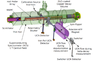
Figure 1: Schematic diagram showing the primary components of the UCNA experiment, including the 7 T polarizing magnet, the spin flipper, the electron spectrometer, and the UCN detector at the switcher (used for polarization measurements).

After emerging from the source, the UCN were transported along a series of guides through a polarizing solenoidal magnet holley12 where a 7 T peak field provided for spin state selection (by rejecting the low-field seeking spin state). Immediately downstream of the 7 T peak field, the polarizing magnet was designed to have a low-field-gradient 1 T region, along which a birdcage-style adiabatic fast passage (AFP) spin-flipper resonator holley12 was located. The spin-flipper provided the ability to flip the spin of the neutrons presented to the electron spectrometer, important for minimization of various systematic effects in the measurement of the asymmetry.

The polarized UCN that emerged from the polarizer and the AFP spin-flipper region were then transported to a 1 T solenoidal spectrometer plaster08 , where a 3-m long cylindrical decay trap was situated along the spectrometer’s axis. There, the UCN spins were aligned parallel or anti-parallel to the magnetic field direction, and the emitted decay electrons then spiraled along the field lines towards one of two electron detector packages located on the two ends of the spectrometer, providing for the measurement of the asymmetry from the rates of detected electrons in the two detector packages.

When the spectrometer magnet was commissioned in the mid-2000’s, the central 1 T field region was uniform to the level of $\pm 3\times 10^{-4}$ over the length of the UCN decay trap plaster08 . However, over time, due to damage to the magnet’s shim coils (as a result of numerous magnet quenches), the field uniformity was somewhat degraded, resulting in a $\sim 30$ Gauss “field dip” near the center of the decay trap region plaster12 . One important feature of the spectrometer’s field profile is that the field was expanded, such that the UCN decays occurred in the 1 T region, but the electron detectors were located in a 0.6 T field region, which minimized Coulomb backscattering and other effects related to the measurement of the asymmetry.

A little more detail on the asymmetry measurement in the electron spectrometer is as follows. The two electron detector packages consisted of multiwire proportional chambers (MWPCs) ito07 , backed by a plastic scintillator disk plaster08 . The MWPCs, with their orthogonally-oriented cathode planes, provided for a measurement of the center position of the spiraling electron trajectory in both transverse directions, which permitted reconstruction of the transverse coordinates of where the electron originated within the UCN decay volume, important for the definition of a fiducial volume. Light from the plastic scintillator was transported along a series of light guides to four photomultiplier tubes (PMTs). The light from the scintillator provided for a measurement of the decay electron’s energy, and the timing from the scintillators provided for a relative determination of the electron’s initial direction of incidence (in the event the electron backscattered in such a way that it was detected in both scintillator detectors).

It is important to point out that the decay electrons necessarily traversed a number of thin foils between the decay trap and the electron detector packages. In particular, the ends of the decay trap were sealed off with thin foils, the purpose of which was to increase the UCN density in the decay trap, thus increasing the detected rate of neutron decays. Then, the MWPC fill gas (100 Torr of neopentane) was sealed off from the spectrometer vacuum by thin entrance and exit foils.

The thickness of these foils over the course of the running of the experiment, from 2007–2013, is summarized in Table 1. I will emphasize that the experiment evolved from operation in 2007 with decay trap foils consisting of 2.5 $\mu$m thick Mylar coated with 0.3 $\mu$m of Be and 25 $\mu$m thick Mylar MWPC foils, to its final configuration in 2013, in which the decay trap foils were reduced to 0.15 $\mu$m thick 6F6F coils hoedl03 coated with 0.15 $\mu$m of Be and 6 $\mu$m thick Mylar MWPC foils.

Table 1: Summary of the decay trap and MWPC foil thicknesses over the course of the running of the UCNA experiment. Prior to the 2012–2013 data taking run, the decay trap foils consisted of Mylar coated with Be (such that, e.g., “2.5 + 0.3” indicates 2.5 $\mu$m of Mylar coated with 0.3 $\mu$m of Be). For the 2012–2013 data taking run, the decay trap foils consisted of 0.15 $\mu$m thick 6F6F foils hoedl03 coated with 0.15 $\mu$m of Be. For all years, the MWPC foils were composed of Mylar.

	Decay Trap	MWPC
Data Set	Foils [$\mu$m]	Foils [$\mu$m]
2007 pattie09	2.5 + 0.3	25
2008–2009 liu10 ; plaster12	0.7 + 0.2 | 13.0 + 0.2	6 | 25
2010 mendenhall13	0.7 + 0.2	6
2011–2012 brown18	0.50 + 0.15	6
2012–2013 brown18	0.15 + 0.15	6

3 Polarization

During the 2011–2012 and 2012–2013 data taking runs, a significant improvement to the systematic error in the determination of the neutron polarization resulted from the installation of a physical shutter in the region between the UCN decay trap and the upstream guide region feeding the spectrometer brown18 . An in-situ measurement of the polarization was carried out on a run-by-run basis following each $\beta$-decay run. The important components to these in-situ measurements of the polarization (see Fig. 1) were the UCN decay volume, the shutter, the guide region feeding the spectrometer, the spin flipper and 7 T polarizer, and then a UCN detector which could be directly connected to the guide region via a switcher.

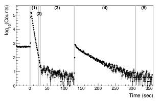
Figure 2: Counts in the UCN detector during the depolarization measurement. See text for details.

A five step procedure for the measurement of the polarization was as follows. In Step (1), following each beta decay run, during which an equilibrium spin state population had developed in the spectrometer (i.e., with the spin flipper operated in some nominal state), the shutter was closed, and the UCN detector was connected to the guide via the switcher. At this point, UCN were trapped by the shutter within the decay volume, while UCN of the nominal spin state upstream of the shutter were drained into the UCN detector. The shutter significantly improved the signal-to-noise ratio for the next steps. In Step (2), the spin flipper state was then toggled from its nominal state during $\beta$-decay running, so that depolarized UCN in the guide region feeding the spectrometer, which were previously trapped by the 7 T polarizing field, had their spins flipped so that they could then transit the 7 T field and then drain into the detector. In Step (3), the shutter was then opened, and with the spin flipper still in its toggled state, depolarized UCN in the decay trap could exit the decay trap region, have their spins flipped permitting them to transit the 7 T field, and then drain into the UCN detector. In Step (4), the spin flipper was reset back to its nominal state, which then permitted a measurement of the polarized UCN within the decay trap. Finally, in Step (5), background data in the detector were taken. Fig. 2 shows an example of counts in the detector during the five step procedure described above.

A series of Monte Carlo simulations were then performed to correct for two effects: a so-called “depolarization evolution” effect, namely that the depolarized population within the decay trap continued to be fed while the shutter was closed, and also a correction for the finite spin flipper efficiency. To study this, simulations were carried out at the NERSC (National Energy Research Scientific Computing Center) facility, in which $\chi^{2}$ searches were performed by varying the guide specularity, Fermi potential, etc. It is important to point out that the systematic error we quote on the polarization (see below) was dominated by the statistical uncertainties in the fitting procedures for the depolarization evolution and finite spin flipper efficiency corrections (i.e., by the counting statistics in the detector). Complete details on the depolarization measurement may be found in Ref. dees-tobepublished .

4 Spectrometer Calibration

The electron detectors were calibrated using a “load lock” system which permitted sealed sources to be translated into the decay trap, and then scanned across the detector face, without breaking vacuum in the spectrometer. The location of this load lock insertion system can be seen in Fig. 1 (denoted “Calibration Source Insertion”). Fig. 3 then illustrates the translation of the sealed sources across the detector, together with an example reconstruction by the MWPC of the transverse $(x,y)$ positions of three different calibration sources (left to right: ²⁰⁷Bi, ¹³⁹Ce, and ¹¹³Sn) within the spectrometer volume.

The thicknesses of the foils encapsulating these three sources were measured in an offline setup using $\alpha$ particles from a collimated ²⁴¹Am source and a silicon detector. A comparison of the measured energy losses in these foils with Geant4 simulations indicated the source foil thicknesses were 9.4 $\mu$m, in contrast with the manufacturer’s nominal specification of 7.6 $\mu$m mendenhall-thesis . These 9.4 $\mu$m thicknesses were then included in the simulations of the energy spectra from the calibration sources.

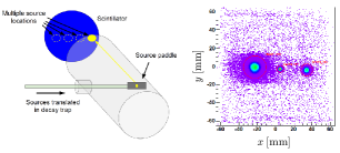
Figure 3: Left: illustration of the “load lock” source insertion system, which permitted sealed sources to be translated across the detector face with the spectrometer under vacuum. Right: example of a reconstruction by the MWPC of the transverse $(x,y)$ positions of three different calibration sources (left to right: ²⁰⁷Bi, ¹³⁹Ce, and ¹¹³Sn).

Calibrations of the so-called “visible energy”, $E_{\mathrm{vis}}$, for each PMT $i$ were carried out according to a model mendenhall-thesis ; brown-thesis in which

$$E_{\mathrm{vis},i}=\eta_{i}^{-1}(x,y)\cdot f_{i}\left(\left(\mathrm{ADC}_{i}-p_{i}(t)\right)\cdot g_{i}(t)\right),$$ (3)

where $\eta_{i}^{-1}(x,y)$ denotes an unfolding of the $(x,y)$-position dependent response of the system (i.e., due to the position-dependent light response of the system), and the function $f_{i}\left(\left(\mathrm{ADC}_{i}-p_{i}(t)\right)\cdot g_{i}(t)\right)$ represents the linearity of the system between light output in the scintillator and the ADC channel ultimately read-out by the data acquisition system for each PMT signal, with $p_{i}(t)$ and $g_{i}(t)$ representing the time-dependent pedestal and gain correction factor, respectively. Values for $\eta_{i}(x,y)$ in multiple $(x,y)$ bins were obtained from special calibration runs carried out with activated xenon gas which uniformly filled the decay trap volume; the calibration especially utilized the endpoint of ¹³⁵Xe decays, whereby the fitted endpoints in each $(x,y)$ bin were compared with a fixed value, thus providing for a relative $\eta_{i}(x,y)$ “position map”. The linearity was obtained from a comparison of the system response to the sources at multiple $(x,y)$ positions, via a comparison of the simulated visible energy multiplied by the $\eta_{i}(x,y)$ position map obtained from the xenon calibration data, with the observed ADC channel number.

A verification of the efficacy of the calibration can be seen in Fig. 4, which compares simulated and reconstructed (i.e., calibrated) spectra for runs with ¹³⁹Ce, ¹¹³Sn, and ²⁰⁷Bi calibration sources. The agreement between simulation and data is seen to be quite good.

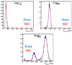
Figure 4: Comparison of simulated (red) and data (blue) spectra from calibration runs with ¹³⁹Ce, ¹¹³Sn, and ²⁰⁷Bi calibration sources.

5 Event Types, Backscattering, and $\langle\cos\theta\rangle$ Corrections

The measurement of the asymmetry requires corrections for a number of different types of backscattering events. Fig. 5 illustrates a classification of the different types of events in the experiment, indicating whether a signal was recorded in each scintillator and/or MWPC. We define “Type 0” events (i.e., those in which there was no reconstructable backscattering) to be the sum of “No Backscattering” events plus “Missed Backscattering” events.

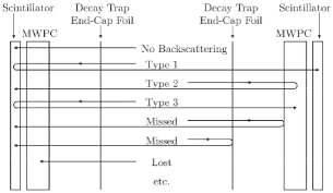
Figure 5: Classification of the different types of events in the experiment.

Corrections for each event type were calculated using independent Geant4 and PENELOPE simulations; the agreement between the simulations was shown to be quite good. We define two types of corrections, each defined such that the corrected asymmetry is $|A_{\mathrm{corr}}|\equiv|A_{\mathrm{uncorr}}|(1+\Delta)$ (i.e., a positive correction $\Delta>0$ indicates that the magnitude of the asymmetry would be increased). The first is a correction we term $\Delta_{2}$, where $\Delta_{2}$ corrects for missed and incorrectly identified backscattering. These types of events would otherwise dilute the asymmetry; therefore, these corrections are expected to be positive. The second is a correction we term $\Delta_{3}$, which we term a $\langle\cos\theta\rangle$ correction. This is so named to account for the deviation of $\langle\cos\theta\rangle$ from a value of 1/2 over each hemisphere, due to the angular-dependent acceptance of the spectrometer and detectors. Because low pitch angle (i.e., large $\cos\theta$) and high-energy events are more likely to be detected, this results in a positive bias to the magnitude of the measured asymmetry; therefore, the values of $\Delta_{3}$ are expected to be negative in order to remove this bias.

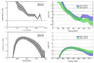
Figure 6: Calculated values of the $\Delta_{2}$ (backscattering, top panels) and $\Delta_{3}$ ($\langle\cos\theta\rangle$, bottom panels) corrections as a function of the electron energy for the 2010 (left panels) and 2011–2012 and 2012–2013 data sets (right panels).

Calculated values for the $\Delta_{2}$ and $\Delta_{3}$ corrections are shown as a function of the electron energy in Fig. 6 for the 2010, 2011–2012, and 2012–2013 data sets. As expected, the magnitude of the corrections decreased as the decay trap and MWPC foil thicknesses progressively decreased with each data set.

Table 2: Summary of the systematic and statistical errors for the 2010, 2011–2012, and 2012–2013 data taking runs. Note that a $+$ ($-$) sign correction indicates the corrections increases (decreases) the magnitude of the asymmetry.

	% Corr.	% Unc.	% Corr.		% Unc.
Effect	2010	2010	2011–2012	2012–2013	2011–2013
Polarization	$+0.67$	$\pm 0.56$	$+0.45$	$+0.34$	$\pm 0.17$
Backscattering	$+1.36$	$\pm 0.34$	$+1.08$	$+0.88$	$\pm 0.30$
$\langle\cos\theta\rangle$	$-1.21$	$\pm 0.30$	$-1.53$	$-1.51$	$\pm 0.33$
Energy Reconstruction	—	$\pm 0.31$	—	—	$\pm 0.20$
Gain Fluctuation	—	$\pm 0.18$	—	—	$\pm 0.16$
Field Nonuniformity	$+0.06$	$\pm 0.10$	—	—	$\pm 0.12$
Muon Veto Efficiency	—	$\pm 0.03$	—	—	$\pm 0.03$
UCN-Induced Background	$+0.01$	$\pm 0.02$	$+0.01$	$+0.01$	$\pm 0.02$
MWPC Efficiency	$+0.12$	$\pm 0.08$	$+0.13$	$+0.11$	$\pm 0.01$
Total Systematics		$\pm 0.82$			$\pm 0.52$
Statistics		$\pm 0.46$			$\pm 0.36$
Recoil Order Effects bilenkii60 ; holstein74 ; wilkinson82 ; gardner01	$-1.71$	$\pm 0.03$	$-1.68$	$-1.67$	$\pm 0.03$
Radiative Effects shann71 ; gluck92	$-0.10$	$\pm 0.05$	$-0.12$	$-0.12$	$\pm 0.05$

6 Error Budgets

A summary of the error budgets for the 2010 mendenhall13 , 2011–2012 brown18 , and 2012–2013 brown18 data sets is shown in Table 2. As already noted above, the significant decrease in the systematic error associated with the polarization resulted from the installation of the shutter in between the 2010 and 2011–2012 data taking runs. Ultimately, as can be seen in the table, the reach of the experiment was limited by the systematic uncertainties in the corrections for backscattering and the $\langle\cos\theta\rangle$ acceptance, both of which were on the scale of the statistical error bar. A future UCNA+ experiment will need to be designed such that these effects are significantly reduced in order for a $<0.2$% precision to be obtained on the asymmetry.

7 Summary of UCNA Results for $A$

A summary of all of the UCNA results for $A$ is given in Table 3. The final result from the combination of the data sets obtained during 2010 mendenhall13 and 2011–2013 brown18 is $A_{0}=-0.12015(34)_{\mathrm{stat}}(63)_{\mathrm{syst}}$.

Table 3: Summary of all results from the UCNA experiment.

Data			Year
Set	$\delta A/A_{\mathrm{stat}}$ [%]	$\delta A/A_{\mathrm{syst}}$ [%]	Published
2007	4.0	1.8	2009 pattie09
2008–2009	0.74	1.1	2010 liu10 ; plaster12
2010	0.46	0.82	2013 mendenhall13
2011–2013	0.37	0.56	2018 brown18

8 Impact of the UCNA Experiment

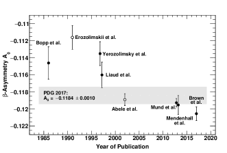
Figure 7: Results for $A$ bopp86 ; yerozolimsky97 ; liaud97 ; abele02 ; mund13 ; mendenhall13 ; brown18 plotted vs. year of publication.

With the UCNA experiment now concluded, the long-term impact of our final result can be seen in Fig. 7. There, one can see the striking landscape of the time evolution of values for $A$ bopp86 ; yerozolimsky97 ; liaud97 ; abele02 ; mund13 ; mendenhall13 ; brown18 , shown plotted vs. publication year. It should be noted that the $\sqrt{\chi^{2}/\nu}$ scale factor the Particle Data Group PDG applies to the error is rather large, $\sim 2.4$, due to the rather striking dichotomy between many of the older and more recent values. A common theme that emerges between many of the older and more recent results concerns the size of the systematic corrections. Generally speaking, in many of the older results, the systematic corrections were of the order of $>2$%, whereas in the more recent results, the corrections were all of the order of $<2$%.

In preparing our most recent publication brown18 , we discovered that the PDG only includes in the calculation of the scale factor those measurements that satisfy $\delta x_{i}<3\sqrt{N}\delta\bar{x}$, where $x_{i}$ refers to one measurement of quantity $x$ out of $N$ measurements and $\delta\bar{x}$ is the non-scaled error on the weighted average $\bar{x}$ PDG . Inclusion of a 0.1% result for $A_{0}$ would remove many of the older results for $A$ from those that enter the calculation of the scale factor. With the expected forthcoming results from the PERKEO III experiment, this could be a real turning point in progress for the field, whereby the PDG may potentially no longer need to apply a $\sqrt{\chi^{2}/\nu}$ scale factor to the average value of $A$.

9 Acknowledgments

This work was supported in part by the U.S. Department of Energy, Office of Nuclear Physics (DE-FG02-08ER41557, DE-SC0014622, DE-FG02-97ER41042) and the National Science Foundation (NSF-0700491, NSF-1002814, NSF-1005233, NSF-1102511, NSF-1205977, NSF-1306997, NSF-1307426, NSF-1506459, and NSF-1615153). We gratefully acknowledge the support of the LDRD program (20110043DR), and the LANSCE and AOT divisions of the Los Alamos National Laboratory.

We thank the organizers of the PPNS-2018 workshop for selecting this abstract for an oral presentation, and for their excellent hospitality during this outstanding decennial workshop.

References

- (1) M. González-Alonso, these proceedings.
- (2) R. W. Pattie et al. (UCNA Collaboration), Phys. Rev. Lett. 102, 012301 (2009).
- (3) J. Liu et al. (UCNA Collaboration), Phys. Rev. Lett. 105, 181803 (2010).
- (4) B. Plaster et al. (UCNA Collaboration), Phys. Rev. A 86, 055501 (2012).
- (5) M. P. Mendenhall et al. (UCNA Collaboration), Phys. Rev. C 87, 032501 (2013).
- (6) M. A.-P. Brown et al. (UCNA Collaboration), Phys. Rev. C 97, 035505 (2018).
- (7) J. D. Jackson, S. B. Treiman, and H. W. Wyld Jr. Physical Review 106, 517 (1957).
- (8) A. Saunders et al. (UCNA Collaboration), Rev. Sci. Instr. 84, 013304 (2013).
- (9) T. M. Ito et al., Phys. Rev. C 97, 012501 (2018).
- (10) H. Saul, these proceedings.
- (11) B. Märkisch et al., arXiv:1812.04666.
- (12) A. T. Holley et al., Rev. Sci. Instrum. 83, 073505 (2012).
- (13) B. Plaster et al., Nucl. Instrum. Methods Phys. Res. A 595, 587 (2008).
- (14) T. Ito et al., Nucl. Instrum. Methods Phys. Res. A 571, 676 (2007).
- (15) S. Hoedl, “Novel Proton Detectors, Ultra-Cold Neutron Decay and Electron Backscatter”, Ph.D. Thesis, Princeton University (2003).
- (16) E. B. Dees et al., in preparation.
- (17) M. P. Mendenhall, “Measurement of the Neutron Beta Decay Asymmetry Using Ultracold Neutrons”, Ph.D. Thesis, California Institute of Technology (2014).
- (18) M. A.-P. Brown, “Determination of the Neutron Beta-Decay Asymmetry Parameter Using Polarized Ultracold Neutrons”, Ph.D. Thesis, University of Kentucky (2018).
- (19) S. M. Bilen’kiĭ et al., Sov. Phys. JETP USSR 10, 1241 (1960) [Zh. Eksp. Teor. Fiz. 37, 1758 (1960)].
- (20) B. R. Holstein, Rev. Mod. Phys. 46, 789 (1974).
- (21) D. H. Wilkinson, Nucl. Phys. A 377, 474 (1982)
- (22) S. Gardner and C. Zhang, Phys. Rev. Lett. 86, 5666 (2001)
- (23) R. T. Shann, Il Nuovo Cimento 5 A, 591 (1971).
- (24) F. Glück and K. Tóth, Phys. Rev. D 46, 2090 (1992)
- (25) M. Tanabashi et al. (Particle Data Group), Phys. Rev. D 98, 030001 (2018).
- (26) P. Bopp et al., Phys. Rev. Lett. 56, 919 (1986).
- (27) B. Yerozolimsky et al., Phys. Lett. B 412, 240 (1997).
- (28) P. Liaud et al., Nucl. Phys. A 612, 53 (1997).
- (29) H. Abele et al., Phys. Rev. Lett. 88, 211801 (2002).
- (30) D. Mund et al., Phys. Rev. Lett. 110, 172502 (2013).