Thick shell regime in the chameleon two-body problem

Abstract

In a previous paper Kraiselburd et al. (2018) we pointed out some shortcomings of the standard approach to chameleon theories consisting in treating the small bodies used to test the Weak Equivalence Principle (WEP) as test particles, whose presence do not modify the chameleon field configuration. In that paper we developed an alternative method to determine the relevant field configuration which takes into account the influence of both test and source bodies, and computed the chamaleon mediated force. Relying on that analysis we showed that the effective acceleration of test bodies is composition dependent even when the model is based on universal couplings. In this paper, we improve our method by using a more suitable approximation for the effective chameleon potential in situations where the bodies are in the so called “thick shell regime”. We then find new and more restrictive bounds on the model’s parametres by confronting the new theoretical predictions with the empirical bounds on Eötvös parameter comming from the Lunar Laser Ranging experiments.

I INTRODUCTION

The realization that a dark sector of physics that is essentially undetected except for is gravitational signatures has led physicists to contemplate the existence of various new kinds of fields beyond what it is found in the Standard Model of Particle Physics. Among these are scalar fields considered as alternatives to a simple cosmological constant, which is usually invoked to account for the late time accelerated expansion of the universe. One obstacle that such proposals need to face is that if these fields are cosmologically relevant they would naturally tend to generate long range forces among material bodies that would generically led to effective violations of the “universality of free fall”, making them empirically unviable. The scalar field model proposed by Khoury & Weltman Khoury and Weltman (2004a, b) (dubbed chameleon) is an alternative which seems to evade such problem. In this model a scalar field $\varphi$ is responsible for the late time accelerated expansion of the Universe. This scalar field couples nonminimally and nonuniversally to the fundamental matter fields, and minimally to the curvature (in the Einstein frame), and thus the model leads, in principle, to effective violations of the universality of free fall (we will refer to this feature as an effective violation of the Einstein’s Weak Equivalence Principle (WEP) despite the fact that strictly speaking, the theory is in complete accord with general covariance). The key ingredient of this model, which nonetheless, makes it in principle viable, is its seeming ability to evade the stringent experimental bounds on the violation of the WEP. This is tied to the fact that the effective mass of the chameleon depends on the density of the medium where the field propagates and therefore the model develops screening or thin shell effects that can in principle suppress the experimental violations of the WEP.

The model has been previously scrutinized by several authorsBrax et al. (2004); Mota and Shaw (2007); Hui et al. (2009); Brax et al. (2010); Brax and Burrage (2011); Khoury (2013). Those works indicate that the model deals successfully with the stringent bounds on the experimental violation of the WEP that are imposed by several observations within the Solar System, including the laboratory experiments performed on Earth, like the Eot-Wash torsion balance Schlamminger et al. (2008), and the Lunar Laser Ranging experimentW Murphy (2013). The point is that the chameleon model predicts that in regions of high-density contrast a screening effect accounts for suppressing the propagation of the field due to the presence of thin-shell effects, while in environments with a low-density contrast the chameleon field is enhanced due to the presence of thick-shell (or “unscreened”) effects. Thus, the thin-shell suppression allows the chameleon model to evade the bounds on the WEP for certain values of its parameters.

In most of the previous works found in the literature the chameleon field is studied as a single-body problem, with an environment using suitable “linear” approximations for the chameleon effective potential. We call this method, the standard approach. These approximations are in good agreement with the numerical solutions to the full nonlinear one-body problem, but they explicitly neglect the effects on the field by the test bodies themselves. Such effects might be quite important given the inherent nonlinearity of the chameleon equation. Once the field profile is obtained, the next step is to estimate the force acting on a test body, which, under the standard approach, is computed by considering the gradient of the scalar field previously obtained, and making use of a heuristic argument (rather than a direct methodical calculation) that relies on approximations associated with the size and composition of the particular test body under consideration to determine its effective charge, and thus proceed to estimate the force as a product of such charge with the previously computed field’s gradient. Again, the nonlinearity of the chameleon equation indicates that such an approach might not produce completely accurate predictions.

The standard approach relies heavily on the consideration of two regimes: a) the thin shell regime where the field settles near the two minima of the effective potential (inside and outside the body) except within a thin region (or shell) inside the body near its surface, where the field interpolates between the two minima; b) the thick shell regime where the field inside the body is close to the minima of the effective potential associated with the environment. In this regime the effective potential is dominated by the linear contribution that is proportional to the density of the body to which the chameleon couples. As we emphasized above, in the thin shell regime violations of the WEP are supposed to be strongly suppressed, but not in the thick shell regime. However, we must keep in mind that those approximations would be 100$\%$ accurate only in some unphysical limits (infinite or zero size bodies), and thus, depending on the accuracy one is interested in, deviations from the estimates resulting from standard approach might occur.

The analytic treatments in the two regimes require different approximations for the effective chameleon potential. According to the standard approach, in the thick shell regime the chameleon force on a test body is not suppressed and is composition dependent when the chameleon coupling to matter $\beta$ is not universal. Given that in the standard approach the test bodies are treated as point-like particles the differential acceleration between the test bodies is proportional to the difference between their corresponding chameleon couplings $|\beta_{1}-\beta_{2}|$. The constant of proportionality is related to the bulk properties of the large body, such as its mass $M_{c}$, size $R_{c}$, coupling $\beta$ and most importantly, it is related to its thin-(thick) shell parameter $\Delta R_{c}/R_{c}$. Thus, provided $\Delta R_{c}/R_{c}\ll 1$, the difference $|\beta_{1}-\beta_{2}|$, which (barring fine tunings) is expected to be of order one, is suppressed by the small factor $\Delta R_{c}/R_{c}$ in such a way that the Eötvos parameter $\eta=2|a_{1}-a_{2}|/(a_{1}+a_{2})$ satisfies the bound $\eta\leq 10^{-13}$ arising from the Eöt-Wash experiments Schlamminger et al. (2008) . Conversely, if $\Delta R_{c}/R_{c}\sim 1$ the chameleon force becomes macroscopically significant and would have been detected by existing experiments. Since this is not the case, the model requires a fortiori the thin shell effects to avoid the observational constraints. Only then the model can be considered as a serious candidate for explaining the current accelerated expansion of the Universe.

In the standard approach, test bodies are treated as point-like particles and therefore the chameleon field (from which the force is derived) is computed considering just the source body. If one did not account in any way for the fact that actual test bodies are not truly point-like, it is clear that (assuming a universal coupling scenario) the resulting estimates for the chameleon mediated force would turn out to be composition independent leading to identically vanishing estimates for the Eötvös parameters. In order to deal with the test bodies’ finite size, the standard approach prescribes the introduction of a “form factor” correcting the computed force of a point-particle Khoury and Weltman (2004b). This cannot be considered as a truly reliable and satisfactory treatment of the issue, and should be regarded instead as just a well motivated method for extracting an estimate of the force. It is clear that what is required is a method that permits the explicit computation of the force that takes into account from the start the fact that actual experiments are preformed with finite size test bodies.

Thus, in order to obtain a more realistic estimate for the chameleon force between a source or “large” body and a small “test” body, an analysis based on two-body characterization of problem is required. That is, we need a treatment in which both the effects of the large and small bodies are taken into account when solving for the chameleon field. Under the two-body treatment the resulting chameleon force should generate directly and automatically the thin-(thick) shell pre-factors associated with each of the two bodies (the large and the small ones) and also exhibit any dependence of the force on the corresponding values of $\beta$’s and other possible characteristics of the bodies. Moreover, within the two-body treatment one should be able to clarify whether under the assumption of a universal-coupling (the one that is considered in most of the previous papers) the parameter $\eta$ really vanishes or not and, if not, what is the remaining composition dependence that arises due to the actual extended nature of all objects involved. This is precisely what we have set to achieve in a previous analysis Kraiselburd et al. (2018) by solving the chameleon field equation in the presence of two bodies. This involves solving in principle a highly nonlinear elliptic equation with complicated boundary conditions. We limited our analysis in several aspects in order to make the problem manageable: 1) The effective chameleon potential was approximated quadratically around their minima, one for each medium (the bodies and the environment that surrounds them), 2) The bodies were assumed to be of constant density; 3) The effects of gravitation on the chameleon field equations were ignored; 4) The large and the test bodies were assumed to be perfectly spherical; 5) The self-gravitation of the test body was neglected; 6) In setups that includes metal encasings around the test bodies the encasing was modeled crudely by a concentric shell of high density. Among these limitations, the first one was clearly unsuitable in situations where the chameleon does not “penetrate” deep into the effective potential associated with interior of the bodies. This situation corresponds to a body with a thick shell and, in that case, the field inside the body is far from its corresponding minimum, but very close to the effective minimum associated with the environment. Then, the field interpolates between the environment’s minimum $\varphi^{\rm out}_{\rm min}$ (at spatial infinity) and the value at the center of the body which is very close to $\varphi^{\rm out}_{\rm min}$. Clearly the quadratic approximation we used previously breaks down in the situations where the thick shell condition applies. The goal of this paper is to overcome this limitation and to better approximate the potential inside the bodies in the appropriate situations. Since the potential in this regime is dominated by the term $\beta\rho\varphi/M_{pl}$, taking $\rho=$constant, we are led to a linear approximation. In the standard approach and for the single body problem this approximation has been proven to be a very good one when compared with the numerical solution to the nonlinear problem Khoury and Weltman (2004a, b). In our methodology we do not attempt to compare with a numerical solution to the full nonlinear problem simply because a numerical treatment of the two-body represents a rather complicated task. Instead we use a simple criterion based on an energy minimization argument to determine among various treatments which one offers the best accuracy for possible approximate solutions of the chameleon equation. In Kraiselburd et al. (2018) we computed and compared this energy for the two-body and for the standard (one body) approaches and looked for the minimum of the two energies. We concluded that our two-body approach provides better results than the standard approach whenever the thin-shell regimes are present in the two bodies. However, when the large body had a thick-shell, the standard approach turned out to be a better suited one. As remarked above, in this paper we improve our two-body calculation and implement the linear approximation for the effective potential in the thick-shell regime. By comparing the energy of the improved solution with that of the single-body problem we find that this time the two-body treatment is better. Moreover, we show that the resulting force remains composition dependent even when universal couplings are assumed, a feature that was already present in our previous analysis Kraiselburd et al. (2018).

The article is organized as follows; in Section II we present the details of the chameleon model and summarize the standard (single body) approach. We also present the solution for the two body problem (obtained in our previous paperKraiselburd et al. (2018)) and an improved solution for the same problem with the approximation for the chameleon field’s effective potential which is appropriate for the thick shell situation. In Sec. III we briefly review the energy criterion proposed in Ref.Kraiselburd et al. (2018) an apply it to the situation at hand. In Sect. IV and V, we analyze the chameleon force between two bodies, compute the theoretical predictions for the Eötvös parameter and, as an example confront them with one specific experimental setup, the Lunar Laser Ranging (LLR). Finally, in Section VI we present our conclusions.

II CHAMELEON MODEL

The chameleon model involves a scalar-field $\varphi$ that couples minimally to gravity via a fiducial metric $g_{\mu\nu}$ (in the Einstein frame), but nonminimally and nonuniversally to the matter sector. The total action is

$$S_{T} = \int d^{4}x\sqrt{-g}\left[\frac{M_{pl}^{2}}{2}R-\frac{1}{2}g^{\mu\nu}(\nabla_{\mu}\varphi)(\nabla_{\nu}\varphi)-V(\varphi)\right]$$ (1)

$$- \int d^{4}xL_{m}\left(\Psi_{m}^{(i)},g_{\mu\nu}^{(i)}\right),$$

where $M_{pl}=1/{\sqrt{8\pi G}}$ and $R$ are the reduced Planck mass and the Ricci scalar associated with $g_{\mu\nu}$ respectively. Each specie $i$ of the matter fields $\Psi_{m}^{(i)}$ couples minimally to a metric $g_{\mu\nu}^{(i)}$ which is related to the Einstein-frame metric $g_{\mu\nu}$ by a conformal factor $g_{\mu\nu}^{(i)}=\exp{\left[\frac{2\beta_{i}\varphi}{M_{pl}}\right]}g_{\mu\nu}$, being $\beta_{i}$ the corresponding dimensionless coupling constant between each specie of matter field $\Psi_{m}^{(i)}$ and the chameleon field. In order to simplify the calculations we will focus only on the case of a universal coupling $\beta_{i}=\beta$ in the analysis for the chameleon force between a source body and a test body, unless otherwise explicitly stated. As we will see, even in this scenario, the resulting force is composition dependent which can be understood by noting that variation of the density imply that bodies of the same mass have different size which lead to different shapes for the chamaleon field, and thus different exerted forces.

Like in previous analyses Khoury and Weltman (2004a, b); Mota and Shaw (2007); Khoury (2013), the model is characterized by a fundamental potential of runaway type, specifically $V(\varphi)=\lambda M^{4+n}\varphi^{-n}$ where $M$ is a constant that has units of mass, $n$ is an positive or negative integer number, and for convenience, and following standard practice, $\lambda=1$ for all values of $n$ except when $n=-4$ when $\lambda=\frac{1}{4!}$.

The energy-momentum tensor (EMT) for each matter component, $T^{m\vspace{5mm}(i)}_{\mu\nu}$, is related with the EMT associated with the Einstein via $T^{m\vspace{5mm}(i)}_{\mu\nu}=\Big{(}2/\sqrt{-g^{(i)}}\Big{)}\delta L_{m}/\delta g^{\mu\nu}_{(i)}=\exp\left[\frac{-2\beta\varphi}{M_{pl}}\right]T^{m}_{\mu\nu}$. Then, the relationship between the traces of both EMT’s is given by $T^{m\vspace{5mm}(i)}=g^{\mu\nu}_{(i)}T^{m\vspace{5mm}(i)}_{\mu\nu}=\exp\left[\frac{-4\beta\varphi}{M_{pl}}\right]g^{\mu\nu}T^{m}_{\mu\nu}=\exp\left[\frac{-4\beta_{\varphi}}{M_{pl}}\right]T^{m}$; and a perfect-fluid and a nonrelativistic matter description is assumed for $T^{m}_{\mu\nu}$ ($T^{m}\approx-\rho$). From Eq. (1),

$$\Box\varphi=\frac{\partial V_{\rm eff}}{\partial\varphi},$$ (2)

where

$$V_{\rm eff}=V(\varphi)+\rho\beta\varphi/M_{pl}$$ (3)

represents the effective potential for each medium of density $\rho$ (the bodies and the environment) which has a minimum if $\beta>0$. Both, the value of the field at the minimum of the effective potential $V_{\rm eff}$ ($\varphi_{\rm min}$) and the mass of the field (the second derivative at that minimum) $\mu_{\rm min}^{2}=\partial^{2}_{\varphi\varphi}V_{\rm eff}(\varphi_{\rm min})$ depend on the density $\rho$. More specifically $\varphi_{\rm min}$ decreases and $\mu_{\rm min}$ increases with the density.

II.1 Standard approach

Let us now consider the standard approach used to calculate the chameleon field of a single body, which was developed by several authors in the past Khoury and Weltman (2004a, b); Waterhouse (2006); Tamaki and Tsujikawa (2008); Khoury (2013). This analysis is restricted to the case where the body is considered to be static with respect to its environment and is taken to be spherically symmetric with radius $R_{c}$, and with homogeneous density $\rho_{\rm in}$. Thus its mass is simply $M_{c}=4\pi\rho_{\rm in}R^{3}_{c}/3$. Furthermore, the body is immersed in a environment of homogeneous density $\rho_{\rm out}$. Ignoring the backreaction of the metric Eq. (2) reads

$$\frac{d^{2}\varphi}{dr^{2}}+\frac{2}{r}\frac{d\varphi}{dr}=V_{,\varphi}+\frac{\beta}{M_{pl}}\rho(r).$$ (4)

Inside the body with density $\rho_{\rm in}$, the value of $\varphi$ at its minimum is denoted by $\varphi^{\rm in}_{\rm min}$, and $\mu_{\rm in}$ will denote its effective mass, while $\varphi_{\infty}$ and $\mu_{\rm out}$ will denote the corresponding values associated with the environment of density $\rho_{\rm out}$ (i.e. outside the body). The boundary (regularity) conditions required to solve the chameleon equation are: i) $\varphi$ and its derivatives are bounded at the origin (for instance, $d\varphi/dr=0$ at $r=0$), ii) the force produced by $\varphi$ on a test particle vanishes at infinity ($\varphi\to\varphi_{\infty}$ as $r\to\infty$), and iii) $\varphi$ and $d\varphi/dr$ should be continuous, in particular at the boundary between the body and its environment.

It turns out that well inside “large” objects with $\rho_{\rm in}\gg\rho_{\rm out}$, in a region $0\leq r\leq R_{c}-\Delta R_{c}$ the field is $\varphi\approx\varphi^{\rm in}_{\rm min}$, and it is only within a thin shell of thickness $\Delta R_{c}$ near the surface of the body, i.e. in the radial domain $R_{c}-\Delta R_{c}\leq r\leq R_{c}$, that the behavior of the field becomes nontrivial.

Within that a thin shell, and to a very good approximation, $\varphi$ grows exponentially until it reaches its boundary at $r=R_{c}$ where it matches continuously the exterior solution. On the other hand, outside the object the field behaves in a typical Yukawa form,

$$\varphi(r)\approx-\Big{(}\frac{\beta}{4\pi M_{pl}}\Big{)}\Big{(}\frac{3\Delta R_{c}}{R_{c}}\Big{)}\frac{M_{c}e^{-\mu_{\rm out}(r-R_{C})}}{r}+\varphi_{\infty},$$ (5)

where

$$\frac{\Delta R_{c}}{R_{c}}\approx\frac{\varphi_{\infty}-\varphi_{\rm in}}{6\beta M_{pl}\Phi_{N}},$$ (6)

and $\Phi_{N}=M_{c}/8\pi M^{2}_{pl}R_{c}$ is the Newtonian potential of the body. The thin-shell condition corresponds to $\Delta R_{c}/R_{c}\ll 1$ (details leading to Eq. (6) can be found in Khoury and Weltman (2004a); Waterhouse (2006); Tamaki and Tsujikawa (2008)). On the other hand, when the body has a thick shell, i.e., $\Delta R_{c}/R_{c}\gtrsim 1$, the value of the chameleon field does not change significantly inside and outside the body, with value $\varphi\approx\varphi_{\infty}$. This situation is typical for a small source body and the chameleon field becomes a small perturbation of the exterior solution. For instance, the exterior solution for a body with thick shell is,

$$\varphi(r)\approx-\Big{(}\frac{\beta}{4\pi M_{pl}}\Big{)}\frac{M_{c}e^{-\mu_{\rm out}(r-R_{C})}}{r}+\varphi_{\infty}.$$ (7)

and the interior solution interpolates between a value $\varphi(r=0)$ and $\varphi(r=R_{c})$ which is very close to $\varphi_{\infty}$ in all the interior. As illustrated by Eq.(5), the thin shell condition is associated with a field $\varphi$ whose difference with $\varphi_{\infty}$ is largely suppressed (i.e. screened) outside the object, and its gradients vanish almost everywhere (except within the thin shell) leading then to a chameleon force that is very small and that barely depends on the composition of the body . This is basically the summary of the understanding of the situation as provided by the standard approach.

II.2 Two-body chameleon approach

In contrast with the standard approach where a test body is treated as a point-like particle, and therefore, its backreaction on the chameleon field is neglected, our method considers the chameleon field generated by two spherical bodies of different and finite size (see Fig.1) Kraiselburd et al. (2018). One of the bodies corresponds to a large body, which we take as the main source for the gravitational field, and a small test body whose backreaction on the chameleon field is taken into account, so that the chamaleon mediated force might be more realistically computed. In the analysis carried out in  Kraiselburd et al. (2018) the effective potential was approximated quadratically around each minima (inside and outside the two bodies): $V_{\rm eff}(\varphi)\simeq V_{\rm eff}(\varphi_{\rm min})+\partial_{\varphi\varphi}V_{\rm eff}(\varphi_{\rm min})[\varphi-\varphi_{\rm min}]^{2}/2$, and the problem was studied making use of the axially symmetric of the situation so the solution for Eq. (2) was described as follows:

$$\quad\varphi=\begin{cases}\varphi_{\rm in1}=\sum\limits_{lm}C_{lm}^{\rm in1}i_{l}(\mu_{1}r)Y_{lm}(\theta,\phi)+\varphi_{1\rm min}^{\rm in}\hskip 149.37697pt(0\leq r\leq R_{1})\\ \varphi_{\rm out}=\sum\limits_{lm}C_{lm}^{\rm out1}k_{l}(\mu_{\rm out}r)Y_{lm}(\theta,\phi)+C_{lm}^{\rm out2}k_{l}(\mu_{\rm out}r^{\prime})Y_{lm}(\theta^{\prime},\phi^{\prime})+\varphi_{\infty}\hskip 19.91684pt(\rm exterior\,\,solution)\\ \varphi_{\rm in2}=\sum\limits_{lm}C_{lm}^{\rm in2}i_{l}(\mu_{2}r^{\prime})Y_{lm}(\theta^{\prime},\phi^{\prime})+\varphi_{2\rm min}^{\rm in}\hskip 139.41832pt(0\leq r^{\prime}\leq R_{2})\end{cases}$$ (8)

where $R_{1}$ and $R_{2}$ are the radii of the large and test bodies, respectively, and $i_{l}$ and $k_{l}$ are the Modified Spherical Bessel Functions (MSBF). The chameleon field is described in two coordinate systems: $(r,\theta,\phi)$ centered in body 1 (large), and $(r^{\prime},\theta^{\prime},\phi^{\prime})$ centered in body 2 (test). Making use of the axial symmetry of the problem, the $z-$axis is established in such a way that it contains the centers of the two bodies, being $D$ the distance between them (see Fig. 1). Therefore, the coordinate transformation is a translation along this axis ($\vec{r}={\vec{r}}^{\,\prime}+D\hat{z}$) so $\theta_{D}=0$, and also $\phi_{D}$ becomes irrelevant due to the axial symmetry ($m=0$). The parameters $C_{lm}^{\rm in1}$, $C_{lm}^{\rm in2}$, $C_{lm}^{\rm out1}$ and $C_{lm}^{\rm out2}$ are determined from the boundary conditions $\varphi_{\rm in1}(R_{1})=\varphi_{\rm out}(R_{1})$, $\partial_{r}\varphi_{\rm in1}(R_{1})=\partial_{r}\varphi^{\prime}_{\rm out}(R_{1})$, $\varphi_{\rm in2}(R_{2})=\varphi_{\rm out}(R_{2})$ and $\partial_{r^{\prime}}\varphi^{\prime}_{\rm in2}(R_{2})=\partial_{r^{\prime}}\varphi^{\prime}_{\rm out}(R_{2})$ by using translation coefficients $\alpha^{lm}_{vw}$ and $\alpha^{*lm}_{vw}$ (see Kraiselburd et al. (2018) for a full description of the method). Furthermore, we found the energy functional associated with the chameleon solution $U_{\rm eff}[\varphi,\rho,D,\beta]$, which upon extremization leads to the correct equation for the static configuration. That minimal value, which naturally depends on the distance between the centers of the two bodies $D$, can be used to compute the chameleon force between the two bodies as $F_{\varphi}=-\partial U_{\rm eff}/\partial D$. In the limit where the size of the test body $R_{2}\rightarrow 0$, i.e., in the point-particle limit, that force reduces to the usual chameleon force $F_{\varphi}\sim\beta_{\rm eff}\nabla\varphi$, where $\beta_{\rm eff}$ is the chameleon coupling to the test body, and the gradient is evaluated at its position. In this case the solution $\varphi$ depends on the coupling $\beta$ between the chameleon and the source body, and thus, the force is proportional to $\beta\beta_{\rm eff}$. This method allows us to find the differential acceleration produced by the chameleon force on two test bodies of different compositionKraiselburd et al. (2018).

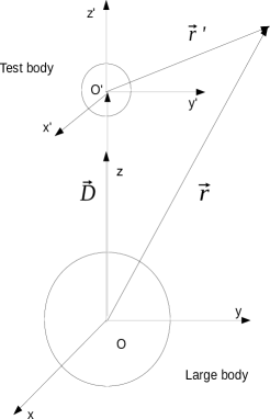
Figure 1: Two body problem.

Our results indicate that for some choices of the free parameters of the chameleon model, the prediction for the Eötvös parameter is larger than previous estimates obtained from the standard approach Kraiselburd et al. (2018).

II.3 Thick shell regime in the two-body chameleon model

In our previous analysis Kraiselburd et al. (2018), we did not implement the linear approximation $V_{\rm eff}^{\rm in}\sim\rho_{\rm in}\frac{\beta\varphi}{M_{pl}}$ which turns to be better suited than the quadratic approximation when bodies develop a thick shell . In order to determine which of these approximations is the best one, we developed a criterion using a minimization of a suitable energy functional. In  Kraiselburd et al. (2018) we found that the energy criterion favors the two body approach over the standard (one body) approach in scenarios where the large object is not in the thick shell regime, the reverse is true for those situations in which the bodies develop a thick shell. In this paper we address this limitation of our previous work and improve our method by implementing the linear approximation $V_{\rm eff}^{\rm in}\sim\rho_{\rm in}\frac{\beta\varphi}{M_{pl}}$ in scenarios where one or both objects are no longer in the thin shell but in the thick shell regime.

We assume that in the thick shell regime the chameleon equation inside the body becomes,

$$\nabla^{2}\varphi_{\rm in}=\rho_{\rm in}\frac{\beta}{M_{pl}},$$ (9)

while outside $\nabla^{2}\varphi_{\rm out}=\mu_{\rm out}^{2}(\varphi_{\rm out}-\varphi_{\infty})$. According to  Waterhouse (2006), a thick shell is developed inside a body when the following condition is satisfied

$$\mu_{\rm in}^{2}\Big{(}\varphi_{\rm in}(0)-\varphi^{\rm in}_{\rm min}\Big{)}>\rho_{\rm in}\frac{\beta}{M_{pl}},$$ (10)

being $\varphi_{\rm in}$ the solution to Eq. (9). Under those conditions, and as shown in Khoury and Weltman (2004a); Kraiselburd et al. (2018), the second term of the effective potential Eq. (3) dominates over the first one and thus we take $V_{\rm eff}^{\rm in}\sim\rho_{\rm in}\frac{\beta\varphi}{M_{pl}}$. Conversely, when the above condition is not satisfied the body develops a thin shell.

For instance, if the test body is the one that satisfies Eq. (10) we expand the most general solution in complete sets of solutions in the interior and exterior regions of the two bodies as follows:

$$\quad\varphi=\begin{cases}\varphi_{\rm in1}=\sum\limits_{l}C_{l}^{\rm in1}i_{l}(\mu_{1}r)Y_{l0}(\theta,\phi)+\phi_{1\rm min}^{\rm in}\hskip 145.10922pt(0\leq r\leq R_{1})\\ \varphi_{\rm out}=\sum\limits_{l}C_{l}^{\rm out1}k_{l}(\mu_{\rm out}r)Y_{l0}(\theta,\phi)+C_{l}^{\rm out2}k_{l}(\mu_{\rm out}r^{\prime})Y_{l0}(\theta^{\prime},\phi^{\prime})+\varphi_{\infty}\hskip 19.91684pt(\rm exterior\,\,solution)\\ \varphi_{\rm in2}=\sum\limits_{l}C_{l}^{\rm in2}r^{\prime l}Y_{l0}(\theta^{\prime},\phi^{\prime})+r^{\prime 2}\rho_{\rm in2}\frac{\beta}{6\sqrt{\pi}M_{pl}}\hskip 122.34692pt(0\leq r^{\prime}\leq R_{2}).\end{cases}$$ (11)

On the other hand, when both bodies, the large one and the test body, have a thick shell the solution can be expressed as follows:

$$\quad\varphi=\begin{cases}\varphi_{\rm in1}=\sum\limits_{l}C_{l}^{\rm in1}r^{l}Y_{l0}(\theta,\phi)+r^{2}\rho_{\rm in1}\frac{\beta}{6\sqrt{\pi}M_{pl}}\hskip 133.72786pt(0\leq r\leq R_{1})\\ \varphi_{\rm out}=\sum\limits_{l}C_{l}^{\rm out1}k_{l}(\mu_{\rm out}r)Y_{l0}(\theta,\phi)+C_{l}^{\rm out2}k_{l}(\mu_{\rm out}r^{\prime})Y_{l0}(\theta^{\prime},\phi^{\prime})+\varphi_{\infty}\hskip 19.91684pt(\rm exterior\,\,solution)\\ \varphi_{\rm in2}=\sum\limits_{l}C_{l}^{\rm in2}r^{\prime l}Y_{l0}(\theta^{\prime},\phi^{\prime})+r^{\prime 2}\rho_{\rm in2}\frac{\beta}{6\sqrt{\pi}M_{pl}}\hskip 122.34692pt(0\leq r^{\prime}\leq R_{2})\end{cases}$$ (12)

The parameters $C_{l}^{\rm in1}$, $C_{l}^{\rm in2}$, $C_{l}^{\rm out1}$ and $C_{l}^{\rm out2}$ are determined from the boundary conditions at the borders of the two bodies $R_{1}$ and $R_{2}$ using translation coefficients $\alpha^{lm}_{vw}$ and $\alpha^{*lm}_{vw}$ to go from one coordinate system to the other (for details see Ref. Kraiselburd et al. (2018)). In both cases (when the large body has thin shell and the test body does not, and when both of them are in the thick shell regime) these coefficients depend on the composition of both bodies and on the surrounding environment. This means that the “chameleon” acceleration of the test body depends on its composition. Figures 2 and 3 illustrate the behavior of the field $\varphi$ with respect to the test body properties in its vicinity. It can be seen that for different densities (Fig. 2) and radii (Fig. 3) of the test body the field acquires different values. In Figures 2a and 3a the large body (in this case the Sun) has a thin shell while the test body (Earth) has a thick shell with $n=\beta=1$ and $M=10$ eV. Meanwhile, in Figures 2b and 3b both bodies are in the thick shell regime and $n=1$, $\beta=10^{-3}$ and $M=10$ eV. Even though these differences are small, they generate a small, but nonvanishing dependency, of the acceleration, on the test body’s composition.

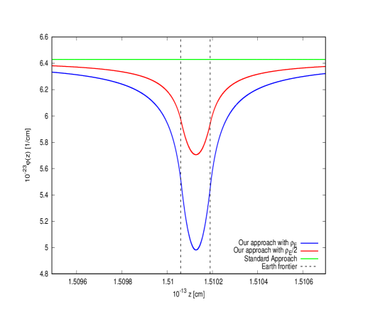
(a) The test body has $thick$ $shell$.

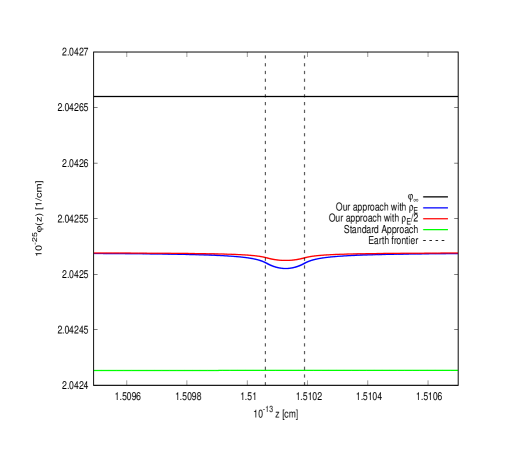
(b) Both bodies (large and test) have $thick$ $shell$.

Figure 2: The chameleon field $\varphi$ as a function of coordinate $z$ inside the test body (Earth) and in its outskirts ($z$ is the distance to the center of the large body (Sun)). The blue lines represet our approach for the Earth while the red ones depict our approach for a test body with the same radius of the Earth but with half of its density. The green lines stand for the standard approach, and the black one, the minimum value of $\varphi$ outside the bodies. Left: The Earth is in the thick shell regime but the Sun is not. Right: Both, Earth and Sun, are in the thick shell regime.

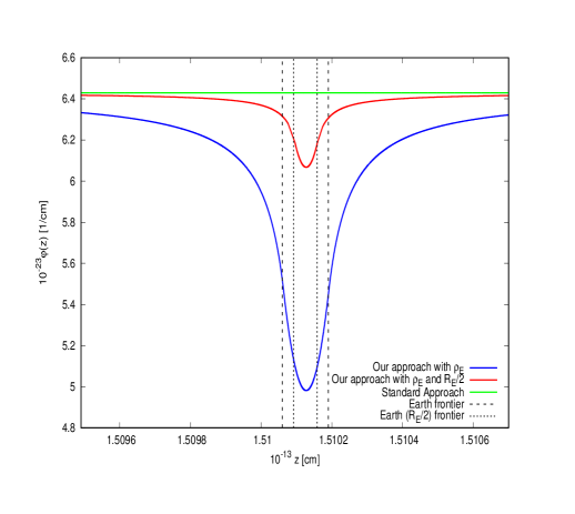
(a) The test body has $thick$ $shell$.

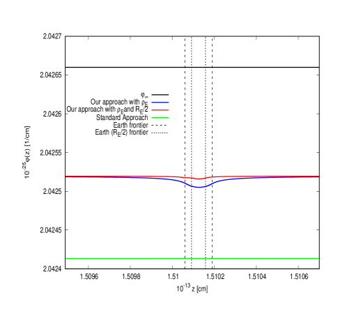
(b) Both bodies (large and test) have $thick$ $shell$.

Figure 3: The chameleon field $\varphi$ as a function of coordinate $z$ inside the test body (Earth) and in its outskirts ($z$ is the distance to the center of the large body (Sun)). The blue lines represent our approach for the Earth while the red ones, our approach for a test body with the same density of the Earth but with half of its radius. The green lines stand for the standard approach, and the black one, the minimum value of $\varphi$ outside the bodies. Left: The Earth is in the thick shell regime but the Sun is not. Right: Both, Earth and Sun, are in the thick shell regime.

III MINIMUM ENERGY CRITERION

We use the energy criterion proposed in Kraiselburd et al. (2018) to evaluate which of the three approximations, the standard approach Khoury and Weltman (2004a); Waterhouse (2006); Tamaki and Tsujikawa (2008), two-body approach with a quadratic effective potential Kraiselburd et al. (2018) or the two-body approach with the thick shell approximation, best characterizes the situations when one or both bodies develop a thick shell, and which correspond to bodies satisfying the condition (10). The criterion relies on the fact that static situations, the field configuration that minimizes the energy functional of a system is also the one that extremizes the action functional associated with that system, and thus, corresponds to the configuration that satisfies the static (classical) equation of motion. Thus, when considering various types of approximations to the solution corresponding to a static field configuration, given the configuration of the objects with which the field interacts, the one with the lowest value of energy functional $U[\varphi,\rho,\beta,D]$ (which is associated with the class of test field configurations) offers the best description of the problem.

The energy associated with the total energy-momentum tensor under the assumptions of staticity and flat space-time is $U=\int_{V}\left(T^{\varphi}_{00}+T^{m}_{00}\right)dV$. However, for the problem at hand, the energy functional that is extremized by the actual field configuration and which leads to Eq. (2) is

$$U_{\rm eff} = \int_{V}\left[\frac{1}{2}(\nabla^{i}\varphi)(\nabla_{i}\varphi)+V_{\rm eff}(\varphi)\right]dV\,\,\,.$$ (13)

We can integrate the above equation by parts and discard the surface terms that vanish at infinity. Moreover, we renormalize the resulting energy functional by subtracting the divergent term associated with the minimum of the effective potential of the environment, obtaining

$$U_{\rm eff}^{*}=\int_{V}\left[-\frac{1}{2}\varphi\nabla^{2}\varphi+V_{\rm eff}(\varphi)-V_{\rm eff}(\varphi_{\rm min}^{\rm out})\right]dV\,\,\,.$$ (14)

As a specific application to our improved approach we analyze a simple experimental scenario: the Lunar Laser Ranging (LLR) where the large body is represented by the Sun and the test bodies by the Earth and the Moon surrounded by the interstellar medium. We remind the reader that for simplicity we assume the bodies and the medium to be perfectly homogeneous. Thus, we compute the functional Eq.(14) for the three approximate methods mentioned above. As emphasized before, under the standard approach Khoury and Weltman (2004a, b), the test body is not taken into account in the determination of the solution for $\varphi$, and therefore a correction factor is introduced by hand in the computation of the chameleon force in order to take into account certain relevant aspects of the test body. For instance, when the test body is considered to have a thin shell, the correction appears in the form of a thin shell parameter $\Delta R/R$ of the test body, or in terms of a factor denoted $Q_{B}$ (see Eqs.(15a) and (15b) below). Other studies Hui et al. (2009); Brax et al. (2010); Burrage et al. (2015) introduce a correction to the solution for $\varphi$ by superposing the exterior solutions for the large and the test bodies but without offering a solution for the field inside the test body (see Kraiselburd et al. (2018) for a thorough discussion on this issue).

Figures 4 and 5 show the energy functional computed for the different approximations (standard approach, two-body approach, two-body approach with thick shell), taking $M=10$ eV, $n=1,2$ and $\rho_{\rm Sun}=1.43\hskip 2.84544pt{\rm g\hskip 2.84544ptcm}^{-3}$, $R_{\rm Sun}=7\times 10^{8}$ m, $\rho_{\rm Earth}=5.5\hskip 2.84544pt{\rm g\hskip 2.84544ptcm}^{-3}$, $R_{\rm Earth}=6.371\times 10^{6}$ m, $\rho_{\rm Moon}=3.34\hskip 2.84544pt{\rm g\hskip 2.84544ptcm}^{-3}$, $R_{\rm Moon}=1.737\times 10^{6}$ m and the interstellar medium density $\rho_{out}=10^{-24}{\rm g\,\ cm^{-3}}$. We appreciate that when the bodies are in the thick shell regime the energy functional is minimized when the improved two-body approach is implemented.

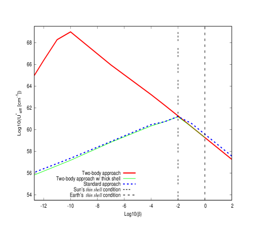
(a) $n=1$

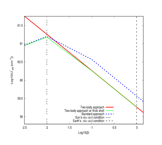
(b) $n=1$ zoom.

Figure 4: Energy functional computed for a setup that mimics the LLR experiment using the two-body approach (red), the two-body approach including the thick shell approximation (green) and the standard one (blue) taking $M=10$ eV and $n=1$. The Sun and the Earth correspond to the large and test bodies, respectively, while the environment represents the interstellar medium. The vertical dotted lines indicate the boundary of the thin shell regime for the Earth and the Sun (values of $\beta$ lower than those indicated by the vertical dotted lines point out that the bodies have a thick shell). The right panel zooms a portion of the left panel. Notice that the energy functional is minimized for the improved two body problem (green line).

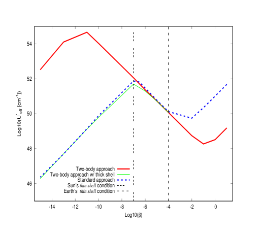
(a) $n=2$

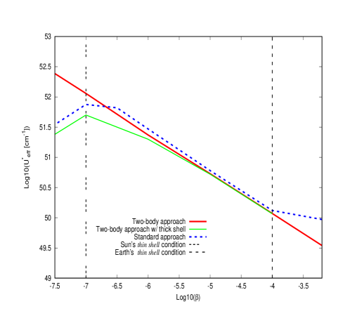
(b) $n=2$ zoom.

Figure 5: Similar to Figure 4 taking $n=2$ .

IV CHAMELEON MEDIATED FORCE BETWEEN TWO SPHERICAL OBJECTS

Under the standard approach Khoury and Weltman (2004a); Hui et al. (2009); Burrage et al. (2015) the chameleon force between a source body $A$ and a test body $B$ is computed from

$$F^{AB}_{\varphi}=2Q_{A}Q_{B}F_{N},$$ (15a)

$$Q_{i}=min\left(\beta,\frac{|\varphi_{\infty}-\varphi^{\rm in}_{i\rm min}|}{2M_{pl}\Phi_{N_{i}}}\right),$$ (15b)

where $i=A,B$, $F_{N}$ refers to the gravitational force between the bodies, and $\Phi_{N_{i}}=\frac{G{\cal{M}}_{i}}{R_{i}}$ refers to the Newtonian potential of the body $i$. When one of the two bodies has a thin shell, the chameleon force is largely suppressed since $Q_{A,B}=\frac{|\varphi_{\infty}-\varphi^{\rm in}_{A,B\rm min}|}{2M_{pl}\Phi_{N_{A,B}}}\ll 1$. However, when the bodies have a thick shell $Q_{A,B}\sim\beta$ (assuming that all the couplings are of the same order), the acceleration on the test body due to the chameleon force turns to be independent of its composition .

IV.1 Chameleon force in the two-body approach

In our previous analysis Kraiselburd et al. (2018) we computed the effective chameleon force between the large and the test body from the first principles using the effective energy functional Eq.(13) for a given configuration as follows: $F_{\rm z\varphi}=-\frac{\partial U_{\rm eff}}{\partial D}$, where $D$ is the distance between the center of the two bodies. After some simplifications, the force reads

$$F_{\rm z\varphi} = F_{\rm z\varphi_{\rm in2}}+F_{\rm z\varphi_{\rm in1}}+F_{\rm z\varphi_{\rm out}}$$ (16)

$$= \frac{\partial}{\partial D}\int_{V_{2}}\Big{\{}\hat{\varphi}_{\rm in2}(\vec{r}^{\,\prime})\Big{[}\frac{(n+1)}{2}\frac{\rho_{2}\beta}{M_{pl}}\Big{]}-\frac{(2+n)\mu_{2}^{2}\hat{\varphi}^{2}_{\rm in2}(\vec{r}^{\,\prime})}{4}\Big{\}}d^{3}{\vec{r}}^{\,\prime}$$

$$+ \frac{\partial}{\partial D}\int_{V_{1}}\Big{\{}\hat{\varphi}_{\rm in1}(\vec{r})\Big{[}\frac{(n+1)}{2}\frac{\rho_{1}\beta}{M_{pl}}\Big{]}-\frac{(2+n)\mu_{1}^{2}\hat{\varphi}^{2}_{\rm in1}(\vec{r})}{4}\Big{\}}d^{3}{\vec{r}}$$

$$+ \frac{\partial}{\partial D}\int_{V_{3}}\Big{\{}\hat{\varphi}_{\rm out}(\vec{r})\Big{[}\frac{(n+1)}{2}\frac{\rho_{\rm out}\beta}{M_{pl}}\Big{]}-\frac{(2+n)\mu_{\rm out}^{2}\hat{\varphi}^{2}_{\rm out}(\vec{r})}{4}\Big{\}}d^{3}{\vec{r}}$$

$$- \frac{\partial}{\partial D}\int_{V_{2}}\Big{\{}\hat{\varphi}_{\rm out}(\vec{r}^{\,\prime})\Big{[}\frac{(n+1)}{2}\frac{\rho_{\rm out}\beta}{M_{pl}}\Big{]}-\frac{(2+n)\mu_{\rm out}^{2}\hat{\varphi}^{2}_{\rm out}(\vec{r}^{\,\prime})}{4}\Big{\}}d^{3}{\vec{r}}^{\,\prime}\;,$$

where ${\hat{\varphi}}=\varphi-\varphi_{\rm min}$. $V_{1}$ represents the region occupied by the large body; $V_{2}$, the region occupied by the test body; while $V_{3}$, the region outside the large body in the coordinate system centered in the large body, the last term compensates for the fact that $V_{3}$, includes the test body:

$$\quad V_{3}=\begin{cases}R_{1}\leq r\leq\infty\\ 0\leq\theta\leq\pi\\ 0\leq\varphi\leq 2\pi\end{cases}$$ (17)

IV.2 Chameleon force in the two-body approach in the thick shell regime

We use a similar expression for the force but by implementing the improved approximation and its solution for the chameleon field as described in Sec. II.3. Thus, when only one of the bodies is in the thick shell regime, for instance, the test body (body 2) the expressions $F_{\rm z\varphi_{\rm in1}}$ and $F_{\rm z\varphi_{\rm out}}$ remain the same as in Eq. (16) except that the solution for $\varphi$ is provided by Eq. (11), and the term that describes the chameleon force inside body 2 is replaced by

$$F_{\rm z\varphi_{\rm in2}}=-\frac{\partial}{\partial D}\int_{V_{2}}\varphi_{\rm in2}(\vec{r}^{\,\prime})\frac{\rho_{2}\beta}{2M_{pl}}d^{3}{\vec{r}}^{\,\prime}\;,$$ (18)

where $\varphi_{\rm in2}$ is the solution given by Eq.(11) for $0\leq r^{\prime}\leq R_{2}$.

However, when both bodies are in the thick shell regime, only the expression $F_{\rm z\varphi_{\rm out}}$ remains the same as in Eq.(16) and the solution for $\varphi$ is provided by Eq.(12) and $F_{\rm z\varphi_{\rm in2}}$ is given by Eq. (18) using Eq. (12) for $\varphi_{\rm in2}$, and $F_{\rm z\varphi_{\rm in1}}$ is replaced by

$$F_{\rm z\varphi_{\rm in1}}=-\frac{\partial}{\partial D}\int_{V_{1}}\varphi_{\rm in1}(\vec{r})\frac{\rho_{1}\beta}{2M_{pl}}d^{3}\vec{r}\;,$$ (19)

where the value of $\varphi_{\rm in1}$ is given by Eq. (12).

V WEP PREDICTIONS

In contrast with the conclusions obtained in the standard approach, and according to our analysis, for universal couplings $\beta$, and in the thick shell regime, the chameleon mediated force does depend in a relevant manner on the composition of test bodies. This dependence is masked in Eqs.(16), (18), (19) but can be seen explicitly in the analytic expressions for the coefficients $C_{l}$ appearing in the expansions (11) and (12) (cf. Kraiselburd et al. (2018)).

In this section, we compute the theoretical prediction for the Eötvös parameter $\eta$ in the LLR scenario and then compare our predictions under the three different kind of approximate methods discussed above. The parameter $\eta=2\frac{|\vec{a_{1}}-\vec{a_{2}}|}{|\vec{a_{1}}+\vec{a_{2}}|}$ is associated with the differential acceleration of two bodies of different composition, where $\vec{a_{i}}=\vec{a}_{i\varphi}+\vec{g}$ ($i=1,2$) is the acceleration of the $i-$test body due to the combined chameleon force $\vec{F}_{i,\varphi}$ and the force of gravity $\vec{F}_{i,g}$, which is basically due to the large body. The acceleration $\vec{a}_{i\varphi}$ is found from the different expressions for the force presented in Sec. IV. It should be noted that in this paper we do not consider the case $M=2.4\times 10^{-3}$ eV, which is associated with the cosmological chameleon , because for this case, and under the relevant conditions, one is almost always in the thin shell regime, and thus, our previous calculations remain valid. As shown in our previous estimations Kraiselburd et al. (2018), the predictions for the LLR experiment (when the bodies are in the thin shell regime) are very similar for both the standard and the two body approach and that their values are below the experimental bound. As the largest value of $\eta$ corresponds to the case $n=1$ and $\beta=10^{-5}$ (in which the Moon looses its thin shell but the Earth and the Sun do not), we can be sure that the predictions for $\eta$ corresponding to all the thick shell regime are much smaller than the experimental bound.

Figure 6 depicts the predictions for $\eta$ based on the LLR experiment using three different approaches: standard, two-body with quadratic effective potential and the improved two-body thick shell approximation. As can be seen in the figure the largest value of the Eötvös parameter is found when one of the test bodies is on the thick shell regime but the other test body is not Hui et al. (2009). This is in agreement with the conclusions of the standard approach. However, in contrast with the latter, and as indicated in Fig.6 the acceleration generated by the chameleon force in test bodies which are in the thick shell regime does depend on their composition (the same happens when the large body develops a thick shell). This result is one of the most important outcomes of this paper. Moreover, the predictions for $\eta$ decrease for lower values of $\beta$ but it does not become null when the thin shell condition does not ensue in the Earth, in contrast with what is predicted by the standard approach. It should be noted that, even though, the predictions for $\eta$ ($n=1$) obtained in this paper are different from Ref.Kraiselburd et al. (2018), the conclusions are the same in that the chameleon model is ruled out for $\beta>10^{-4}$. On the other hand, for $n=2$ the improved two body approach that implements the thick shell approximation is consistent with experimental bounds if $\beta<10^{-3.8}$, contrary to what we found previously using the two body approach with the quadratic approximation for the effective potential.

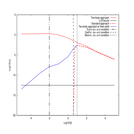
(a) $n=1$

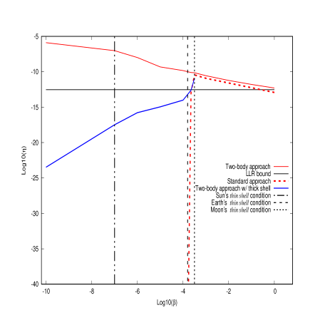
(b) $n=2$

Figure 6: The Eötvös parameter $\eta$ (in ${\rm log_{10}}$ scale) for the LLR experiment as a function of the parameter $\beta$ (in ${\rm log_{10}}$ scale) for different positive values of $n$. All bodies are surrounded by the interstellar medium. ${M=10\hskip 2.84544pt{\rm eV}}$. The vertical lines show the values of $\beta$ below which the thin shell condition is no longer satisfied for the Earth, Moon and Sun. The horizontal line represents the experimental bound W Murphy (2013). For all values computed in this plot, the energy criterion developed in Section III indicates that the two body approach together with an improved approximation to the effective potential provides better results than the standard approach and than the two-body approach with the quadratic approximation for the potential.

VI CONCLUSIONS

In this article we study the chameleon model using a two-body-problem approach devised by us in Kraiselburd et al. (2018), by improving our previous analysis to situations where the thick shell regime becomes relevant. In that regime we thus replace the previously used quadratic approximation for the effective potential (which is not adequate when the field departs largely from its minimum inside the bodies) by a linear one. This analysis amends our previous work Kraiselburd et al. (2018) method in several respects.

First, we find expressions for the chameleon field $\varphi$ when one or both bodies (the test and the large bodies) are in the thick shell regime. Then, we calculate an energy functional and conclude that the energy minimization criterion favors our improved approach over the other ones for the regimes in question.

We also obtain expressions for the chameleon mediated force from first principles and find predictions for the Eötv̈os parameter $\eta$ in a setup that mimics the LLR experiment. We conclude that our improved approach and the standard approach agrees on the predictions for $\eta$ when the chameleon coupling lies in the following ranges $5\gtrsim\beta\gtrsim 10^{2.5}$ for $n=1$ and $1\gtrsim\beta\gtrsim 10^{-3.5}$ for $n=2$ with $M\sim 10$ eV and the prediction is that the Eötvös parameter is in conflict with the observational bounds imposed by the LLR experiments. The largest prediction of $\eta$ (for each $n$) corresponds to scenarios where one of the test bodies is in the thick shell regime but the other is not. For lower values of $\beta$ the test bodies (the Moon and the Earth) and/or the large body (the Sun) are not in the thin shell regime anymore and thus our improved and the standard approaches do not agree. For instance, for $\beta\lesssim 10$ ($n=1$) the standard approach predicts no violation of the experimental bounds for $\eta$, while our improved treatment shows that for $10^{-4}\lesssim\beta\lesssim 10^{4}$ the predicted $\eta$ violates the experimental bounds. Our results allow us then to put further constraints on the parameters $n,\beta,M$ of the original chameleon model. Finally, we stress that in contrast with the conclusions obtained from the standard approach, our treatment shows that test bodies having a thick shell fall with accelerations that are composition dependent. The current and previous analyses Kraiselburd et al. (2018) illustrate the difficulty in considering a sharp distinction between the thin and thick shell regimes. In fact, whenever an approximation is used relying on one or the other regimes or the consideration of the one body problem (standard approach) versus the two body problem (our approach), there is no a priori manner to be sure which one is more appropriate at an arbitrary level of precision. In this regard the energy criteria seems to offer a reliable guidance as to which approximation is more trustworthy.

References

- Kraiselburd et al. (2018) L. Kraiselburd, S. J. Landau, M. Salgado, D. Sudarsky, and H. Vucetich, Phys. Rev. D 97, 104044 (2018).
- Khoury and Weltman (2004a) J. Khoury and A. Weltman, Phys. Rev. D 69, 044026 (2004a).
- Khoury and Weltman (2004b) J. Khoury and A. Weltman, Phys. Rev. Lett. 93, 171104 (2004b).
- Brax et al. (2004) P. Brax, C. van de Bruck, A.-C. Davis, J. Khoury, and A. Weltman, Phys. Rev. D 70, 123518 (2004).
- Mota and Shaw (2007) D. F. Mota and D. J. Shaw, Phys. Rev. D 75, 063501 (2007).
- Hui et al. (2009) L. Hui, A. Nicolis, and C. W. Stubbs, Phys. Rev. D 80, 104002 (2009).
- Brax et al. (2010) P. Brax, C. van de Bruck, D. F. Mota, N. J. Nunes, and H. A. Winther, Phys. Rev. D 82, 083503 (2010).
- Brax and Burrage (2011) P. Brax and C. Burrage, Phys. Rev. D 83, 035020 (2011).
- Khoury (2013) J. Khoury, Class. Quantum Grav. 30, 214004 (2013).
- Schlamminger et al. (2008) S. Schlamminger, K.-Y. Choi, T. A. Wagner, J. H. Gundlach, and E. G. Adelberger, Phys. Rev. Lett. 100, 041101 (2008).
- W Murphy (2013) T. W Murphy, Reports on progress in physics. 76, 076901 (2013).
- Waterhouse (2006) T. P. Waterhouse, ArXiv Astrophysics e-prints (2006), eprint astro-ph/0611816.
- Tamaki and Tsujikawa (2008) T. Tamaki and S. Tsujikawa, Phys. Rev. D 78, 084028 (2008).
- Burrage et al. (2015) C. Burrage, E. J. Copeland, and E. A. Hinds, J. Cosmol. Astropart. Phys. 3, 042 (2015), eprint 1408.1409.