The search for statistical anisotropy in the gravitational-wave background with pulsar timing arrays

Abstract

Pulsar-timing arrays (PTAs) are seeking gravitational waves from supermassive-black-hole binaries, and there are prospects to complement these searches with stellar-astrometry measurements. Theorists still disagree, however, as to whether the local gravitational-wave background will be statistically isotropic, as arises if it is the summed contributions from many SMBH binaries, or whether it exhibits the type of statistical anisotropy that arises if the local background is dominated by a handful (or even one) bright source. Here we derive, using bipolar spherical harmonics, the optimal PTA estimators for statistical anisotropy in the GW background and simple estimates of the detectability of this anisotropy. We provide results on the smallest detectable amplitude of a dipole anisotropy (and several other low-order multipole moments) and also the smallest detectable amplitude of a “beam” of gravitational waves. Results are presented as a function of the signal-to-noise with which the GW signal is detected and as a function of the number of pulsars (assuming uniform distribution on the sky and equal sensitivity per pulsar). We provide results first for measurements with a single time-domain window function and then show how the results are augmented with the inclusion of time-domain information. The approach here is intended to be conceptually straightforward and to complement the results of more detailed (but correspondingly less intuitive) modeling of the actual measurements.

I Introduction

A longstanding effort Foster:1990 ; Maggiore:1999vm ; Burke-Spolaor:2015xpf ; Lommen:2015gbz ; Hobbs:2017oam ; Yunes:2013dva to detect a stochastic gravitational-wave background with pulsar-timing arrays consists now of three major efforts—the Parkes Pulsar Timing Array (PPTA) Hobbs:2013aka ; Manchester:2012za , North American Nanohertz Observatory for Gravitational Waves (NANOGrav) Arzoumanian:2018saf , and the European Pulsar Timing Array (EPTA) Lentati:2015qwp –that collaborate through an International Pulsar Timing Array (IPTA) Verbiest:2016vem . The effects of gravitational waves on the arrival times of pulses from pulsars Detweiler:1979wn ; Sazhin:1978 produce a characteristic angular correlation Hellings:1983fr in the pulsar-timing residuals. Signals at the frequencies $\sim 1$nHz are expected from the mergers of supermassive-black-hole binaries Rajagopal:1994zj ; Jaffe:2002rt . There are also prospects to use complementary information from stellar astrometry Book:2010pf ; Moore:2017ity ; Mihaylov:2018uqm ; OBeirne:2018slh ; Qin:2018yhy as the apparent position of distant stars will oscillate with a characteristic pattern on the sky due to GWs.

It is still not understood, though, whether the local GW signal due to SMBH mergers will be the type of stochastic background that arises as the sum of a large number of cosmological sources, or whether it will be dominated by just a handful—or even just one—source Allen:1996gp ; Sesana:2008xk ; Ravi:2012bz ; Cornish:2013aba ; Kelley:2017vox . Roughly speaking, if there are $\sim N$ Poisson sources contributing to the signal, then the amplitude of anisotropy in the GW background should be $\sim N^{-1/2}$. A first obvious step, after the initial detection of a gravitational-wave signal, will therefore be to seek the anisotropy in the background that may arise from a finite number of sources. Exotic sources might also lead to anisotropy Kuroyanagi:2016ugi .

Prior work Anholm:2008wy ; Mingarelli:2013dsa ; Gair:2014rwa has developed tools to characterize and seek with PTAs anisotropy in the GW background that were then implemented in a null search Taylor:2015udp . This anisotropy was characterized (as it is here also) in terms of an uncorrelated and unpolarized background of gravitational waves with a direction-dependent intensity parametrized in terms of spherical-harmonic expansion of the intensity. Here we re-derive anisotropy-detection tools using mathematical objects (bipolar spherical harmonics; BiPoSHs Hajian:2003qq ; Hajian:2005jh ; Joshi:2009mj ) developed for analogous problems in the study of the cosmic microwave background. The analysis here provides some simplifications and insights and also intuitive estimates for the smallest detectable signals. We provide numerical results for the smallest detectable dipole-anisotropy amplitude as a function of the signal-to-noise with which the isotropic signal is detected and as a function of the number of pulsars in the array. We restrict our attention to PTAs but describe how the detectability will be augmented with the inclusion of astrometry.

This paper is organized as follows: In Section II we describe the idealized observables that we model. In Section III we review the standard Hellings-Downs correlation function (and its harmonic-space equivalent, the timing-residual power spectrum) used to detect the GW background. Section IV introduces the bipolar-spherical-harmonic formalism and describes how to infer the BiPoSH amplitudes from the observables. Section V describes the model of an uncorrelated anisotropic background we consider here (and considered in Refs. Mingarelli:2013dsa ; Gair:2014rwa ) and calculates the BiPoSH coefficients for the model in terms of the model’s anisotropy parameters $g_{LM}$. Section VI derives minimum-variance estimators for the spherical-harmonic coefficients $g_{LM}$ that parametrize the anisotropy and the variances $(\Delta g_{LM})^{2}$ with which they can be measured. Section VII evaluates the smallest detectable anisotropy beginning with a dipole and then generalizing to anisotropies of higher-order multipole moment and then the anisotropy due to a beam of uncorrelated unpolarized gravitational waves from a specific direction. Section VIII describes how the previous results, obtained for a single timing-residual map, are generalized to incorporate the multiple maps that may be obtained from time-domain information. We discuss the extension to astrometry and make closing remarks in Section IX.

II Harmonic and real-space angular observables

PTA measurements are characterized by the temporal evolution of the timing residuals and the dependence of the observables as a function of position on the sky. Here we focus primarily on the angular structure. To simplify, we speak here of the “timing residuals” $z(\hat{n})$ measured in a PTA as a function of position $\hat{n}$ on the sky. These “timing residuals,” in a more complete analysis, will be obtained from some convolution of the timing residuals (TRs) with a time-sequence window function (and there may well be a number of such timing residuals that are obtained from convolutions of the full timing-residual data with different time-sequence window functions—more on this in Section VIII). Strictly speaking, therefore, each appearance of a GW power spectrum $P_{h}(k)$ in the expressions below should be replaced by $P_{h}(k)\left[W(k)\right]^{2}$ where $W(k)$ is an appropriate time-domain window function.

Any such timing residual $z(\hat{n})$ can be expanded

$$z(\hat{n})=\sum_{\ell=2}^{\infty}\sum_{m=-\ell}^{\ell}z_{\ell m}Y_{\ell m}(\hat{n}),$$ (1)

in terms of spherical harmonics $Y_{\ell m}(\hat{n})$, which constitute a complete orthonormal basis for scalar functions on the two-sphere. The expansion coefficients are obtained from the inverse transform,

$$z_{\ell m}=\int\,d^{2}\hat{n}\,z(\hat{n})\,Y_{\ell m}^{*}(\hat{n}).$$ (2)

The sum in Eq. (1) is only over $\ell\geq 2$, as the transverse-traceless gravitational waves that propagate in general relativity give rise only to timing-residual patterns with $\ell\geq 2$. We assume that the timing residuals (convolved with a time-sequence window function) are real, and so $z_{\ell m}^{*}=(-1)^{m}z_{\ell,-m}$. Note that specification of $z(\hat{n})$ is equivalent to specification of $z_{\ell m}$ and vice versa—they are two different ways to describe the same observables.

III Power spectrum and correlation function

The timing residuals $z({\hat{n}},{\hat{k}})$ arising from a gravitational wave with polarization tensor $h_{ab}$ moving in direction ${\hat{k}}$ are given by

$$z(\hat{n};\hat{k})=\frac{n^{a}n^{b}h_{ab}}{2(1+\hat{k}\cdot\hat{n})}\;.$$ (3)

Strictly speaking, the timing residuals are observed as a function of time, but the angular pattern here is that after those time-domain data have been convolved with a time-domain window function so that the resulting map $z(\hat{n})$ is then real.

As discussed in Refs. Roebber:2016jzl ; Qin:2018yhy (and below), the rotationally-invariant observed power spectrum $C_{\ell}\propto\sum_{m}|z_{\ell m}|^{2}/(2\ell+1)$ for this plane wave is

$$C_{\ell}\propto\frac{(\ell-2)!}{(\ell+2)!}.$$ (4)

Since Eq. (3) is a scalar and linear in $h_{ab}$, the timing residuals from any collection of plane waves—i.e., any gravitational-wave signal—will have the power spectrum of Eq. (4). If the timing residuals $z(\hat{n})$ arise from a realization of a statistically isotropic gravitational-wave background, then the spherical-harmonic coefficients $z_{\ell m}$ of the observed $z(\hat{n})$ map will satisfy

$${\left\langle z_{\ell m}z^{*}_{\ell^{\prime}m^{\prime}}\right\rangle}=C_{\ell}\,\delta_{\ell\ell^{\prime}}\delta_{mm^{\prime}},$$ (5)

where the angle brackets denote the average over all realizations of the gravitational-wave background, and $\delta_{\ell\ell^{\prime}}$ and $\delta_{mm^{\prime}}$ are Kronecker deltas. Eq. (5) states that if the GW background is statistically isotropic then all of the $z_{\ell m}$ are uncorrelated and that each $z_{\ell m}$ is some number selected from a distribution of variance $C_{\ell}$. The resulting map, $z(\hat{n})$, is then real after convolution with the appropriate time-domain window function.

The timing-residual power spectrum is related to the rotationally-invariant two-point autocorrelation function (Gair:2014rwa, ),

$$C(\Theta)={\left\langle z(\hat{n})z(\hat{m})\right\rangle}_{\hat{n}\cdot\hat{m}=\cos\Theta}=\sum_{\ell}\frac{2\ell+1}{4\pi}C_{\ell}P_{\ell}(\cos\Theta);$$ (6)

i.e., the product of the timing residuals in two different directions separated by an angle $\Theta$, averaged over all such pairs of directions. The two-point autocorrelation function from a stochastic GW background is the classic Hellings-Downs curve,

$$C(\Theta)\propto(1/2)(1-x)\log\left[\frac{1}{2}(1-x)\right]-\frac{1}{6}\left[\frac{1}{2}(1-x)\right]+\frac{1}{3},$$ (7)

where $x=\cos\Theta$. Again, the two-point autocorrelation function has this form regardless of whether the GW background is statistically isotropic or otherwise.

Since the power spectrum $C_{\ell}$ and two-point autocorrelation function $C(\Theta)$ do not depend on whether the background is isotropic or otherwise, the natural first step in any effort to detect a GW background is to establish from the data that these are nonzero. Formulas to derive $C_{\ell}$ from (idealized) data are provided below.

IV Bipolar spherical harmonics

There is, however, far more information in a map $z(\hat{n})$ (or equivalently, its set of $z_{\ell m}$) than that provided by the timing-residual power spectrum and Hellings-Downs correlation. The most general correlation between any two $z_{\ell m}$s can be written (see, e.g., Ref. Book:2011na ; Pullen:2007tu ),

$${\left\langle z_{\ell m}z^{*}_{\ell^{\prime}m^{\prime}}\right\rangle} = C_{\ell}\delta_{\ell\ell^{\prime}}\delta_{mm^{\prime}}$$

$$+\sum_{L=1}^{\infty}\sum_{M=-L}^{L}(-1)^{m^{\prime}}\langle\ell\,m\,\ell^{\prime},\,-m^{\prime}|LM\rangle A^{LM}_{\ell\ell^{\prime}},$$

where $C_{\ell}$ is the (isotropic) power spectrum introduced above, $\langle\ell\,m\,\ell^{\prime}\,m^{\prime}|LM\rangle$ are Clebsch-Gordan coefficients, and the $A^{LM}_{\ell\ell^{\prime}}$ are BiPoSH coefficients. Note that the power spectrum $C_{\ell}$ can be identified as $(-1)^{\ell}A^{00}_{\ell\ell}/\sqrt{2\ell+1}$.

As Eq. (6) indicates, the Hellings-Downs curve $C(\Theta)$ considers information obtained only from the angular separation $\Theta$ between two directions $\hat{n}$ and $\hat{m}$, but disregards any information about the specific directions $\hat{n}$ and $\hat{m}$. This additional information is parametrized with BiPoSHs in terms of BiPoSH coefficients $A^{LM}_{\ell\ell^{\prime}}$ that characterize departures from statistical isotropy. If there is a dipolar power anisotropy (higher flux of GWs from one direction than from the opposite direction), it is characterized by the $L=1$ (dipolar) BiPoSHs, and the different $M=0,\pm 1$ components provide the spherical-tensor representation of the dipole. A quadrupolar power asymmetry (e.g., as might arise if there were GWs coming from the $\pm\hat{z}$ direction) are characterized by the $L=2$ BiPoSH coefficients, and so forth.

IV.1 Measurement of BiPoSH coefficients

We suppose that the “data” come in the form of a collection of measured values $z_{\ell m}^{\rm data}=z_{\ell m}+z_{\ell m}^{\rm noise}$ each of which has a contribution $z_{\ell m}$ from the signal and another $z_{\ell m}^{\rm noise}$ from measurement noise. We assume that the noise in each $z_{\ell m}^{\rm noise}$ are uncorrelated and that each $z_{\ell m}$ has a variance $N^{zz}$ (which we further assume to be $\ell$-independent – the white-noise power spectrum – a good approximation if the timing-residual noises in all pulsars are comparable).

Estimators for the BiPoSH coefficients are then obtained from

$$\savestack{\tmpbox}{\stretchto{\scaleto{\scalerel*[\widthof{A^{LM}_{\ell\ell^{\prime}}}]{\kern-0.6pt\bigwedge\kern-0.6pt}{\rule[-505.89pt]{4.30554pt}{505.89pt}}}{}}{0.5ex}}\stackon[1pt]{A^{LM}_{\ell\ell^{\prime}}}{\tmpbox}=\sum_{mm^{\prime}}z^{\rm data}_{lm}z^{*\,{\rm data}}_{l^{\prime}m^{\prime}}(-1)^{m^{\prime}}\langle l\,m\,l^{\prime},\,-m^{\prime}|LM\rangle.$$ (9)

This estimator has a variance, under the null hypothesis (for even $L+\ell+\ell^{\prime}$) Book:2011na ,

$${\left\langle\left|\savestack{\tmpbox}{\stretchto{\scaleto{\scalerel*[\widthof{A^{LM}_{\ell\ell^{\prime}}}]{\kern-0.6pt\bigwedge\kern-0.6pt}{\rule[-505.89pt]{4.30554pt}{505.89pt}}}{}}{0.5ex}}\stackon[1pt]{A^{LM}_{\ell\ell^{\prime}}}{\tmpbox}\right|^{2}\right\rangle}=(1+\delta_{\ell\ell^{\prime}})C_{\ell}^{\mathrm{data}}C_{\ell^{\prime}}^{\mathrm{data}},$$ (10)

where $C_{\ell}^{\mathrm{data}}=C_{\ell}+N^{zz}$ is the power spectrum of the map, which includes the signal and the noise. The $\delta_{ll^{\prime}}$ arises since the root-variance to a variance of a Gaussian distribution is $\sqrt{2}$ times the variance. We will see below that we need consider only combinations with even $\ell+\ell^{\prime}+L$. If the map $z(\hat{n})$ is real, then ${A^{LM}_{\ell\ell^{\prime}}=A^{LM}_{\ell^{\prime}\ell}}$ (for even $\ell+\ell^{\prime}+L$), and the estimators $\savestack{\tmpbox}{\stretchto{\scaleto{\scalerel*[\widthof{A^{LM}_{\ell\ell^{\prime}}}]{\kern-0.6pt\bigwedge\kern-0.6pt}{\rule[-505.89pt]{4.30554pt}{505.89pt}}}{}}{0.5ex}}\stackon[1pt]{A^{LM}_{\ell\ell^{\prime}}}{\tmpbox}$ and $\savestack{\tmpbox}{\stretchto{\scaleto{\scalerel*[\widthof{A^{LM}_{\ell^{\prime}\ell}}]{\kern-0.6pt\bigwedge\kern-0.6pt}{\rule[-505.89pt]{4.30554pt}{505.89pt}}}{}}{0.5ex}}\stackon[1pt]{A^{LM}_{\ell^{\prime}\ell}}{\tmpbox}$ are the same. The covariance between any two other different $\savestack{\tmpbox}{\stretchto{\scaleto{\scalerel*[\widthof{A^{LM}_{\ell\ell^{\prime}}}]{\kern-0.6pt\bigwedge\kern-0.6pt}{\rule[-505.89pt]{4.30554pt}{505.89pt}}}{}}{0.5ex}}\stackon[1pt]{A^{LM}_{\ell\ell^{\prime}}}{\tmpbox}$ vanishes.

By setting $L=0$ and identifying $C_{\ell}=(-1)^{\ell}A^{00}_{\ell\ell}/\sqrt{2\ell+1}$, we recover the power-spectrum estimator,

$$\savestack{\tmpbox}{\stretchto{\scaleto{\scalerel*[\widthof{C_{\ell}}]{\kern-0.6pt\bigwedge\kern-0.6pt}{\rule[-505.89pt]{4.30554pt}{505.89pt}}}{}}{0.5ex}}\stackon[1pt]{C_{\ell}}{\tmpbox}=\sum_{m=-\ell}^{\ell}\frac{|z_{\ell m}^{\rm data}|^{2}}{2\ell+1}-N^{zz},$$ (11)

which has a variance

$${\left\langle\left(\Delta C_{\ell}\right)^{2}\right\rangle}=\frac{2}{2\ell+1}\left(C_{\ell}^{\rm data}\right)^{2}.$$ (12)

Under the null hypothesis of no gravitational-wave background (to be distinguished from the null hypothesis of a gravitational-wave background that is isotropic), $C_{\ell}^{\rm data}=N^{zz}$. This result will be used in Eq. (24) below.

V Model and BiPoSH Coefficients

We now focus on understanding the $\ell,\ell^{\prime}$ dependence of the BiPoSH coefficients $A^{LM}_{\ell\ell^{\prime}}$. To do so, we must understand the dependence of the observable $z(\hat{n})$ on the gravitational-wave background.

V.1 Model of anisotropic background

In order to link measurements of the timing residuals to an underlying gravitational wave background, we need a model for the statistics of that background. Although there are an infinitude of ways the background can depart from statistical isotropy, we consider (as did Refs. Mingarelli:2013dsa ; Gair:2014rwa ) here those that can be parametrized as

$${\left\langle h_{s}(\vec{k})h_{s^{\prime}}^{*}(\vec{k}^{\prime})\right\rangle} = \frac{1}{4}\delta_{ss^{\prime}}(2\pi)^{3}\delta_{D}(\vec{k}-\vec{k}^{\prime})P_{h}(k)$$

$$\times\left[1+\sum_{L>0}\sum_{M=-L}^{L}g_{LM}Y_{LM}(\hat{k})\right],$$

where $h_{s}(\vec{k})$ is the amplitude of the gravitational-wave mode with wavevector $\vec{k}$ and polarization $s=+,\times$. With the Dirac delta function in this parametrization, we are still preserving the assumption that different Fourier modes are uncorrelated. We are also assuming that the frequency dependence of the GW background is the same in all directions and that the $+$ and $\times$ modes are still equally populated (i.e., that the background is unpolarized). The sum over spherical harmonics allows, however, for the most general angular dependence of the gravitational-wave flux, parametrized by spherical-harmonic coefficients $g_{LM}$. Here, the gravitational-wave power spectrum is $P_{h}(k)$, and an isotropic background is recovered for $g_{LM}\to 0$ for all $L>0$. In this model, the $g_{LM}$ are the spherical harmonic coefficients of the map of total gravitational-wave power.

Since the term in the brackets in Eq. (LABEL:eqn:generalized) must be positive, the spherical-harmonic coefficients are restricted to be $g_{L0}\leq\sqrt{4\pi/(2L+1)}$, and a roughly similar bound applies to $\sqrt{2}\,\mathrm{Re}g_{LM}$ and $\sqrt{2}\,\mathrm{Im}g_{LM}$ for $M\neq 0$.

V.2 Resulting timing-residual BiPoSH coefficients (and angular power spectrum)

We now calculate the BiPoSH amplitude that arises from a GW background of the form in Eq. (LABEL:eqn:generalized), based on its imprint, Eq. (3). If the GW direction is taken to be $\hat{k}=\hat{z}$, then this becomes

$$z(\hat{n};\hat{k}=\hat{z})=h_{+}(1-\cos\theta)\cos 2\phi+h_{\times}(1-\cos\theta)\sin 2\phi,$$ (14)

where $h_{+}$ and $h_{\times}$ (both most generally complex) are the amplitudes of the $+$ and $\times$ polarizations.

This plane wave is described by spherical-harmonic coefficients,

$$z_{\ell m}(\hat{z}) = z_{\ell}\left[h_{+}(\delta_{m2}+\delta_{m,-2})+ih_{\times}(\delta_{m2}-\delta_{m,-2})\right]$$

$$= z_{\ell}\left[(h_{+}+ih_{\times})\delta_{m2}+(h_{+}-ih_{\times})\delta_{m,-2}\right],$$

where we defined

$$z_{\ell}\equiv(-1)^{\ell}\sqrt{\frac{{4\pi}(2\ell+1)(\ell-2)!}{(\ell+2)!}}\,.$$ (16)

From this result, we can construct the spherical-harmonic coefficients for a plane wave in any other direction. To do so, we write

$$z(\hat{n};\hat{k}) = \sum_{\ell mm^{\prime}}Y_{\ell m}(\hat{n})D^{(l)}_{mm^{\prime}}(\phi_{k},\theta_{k},0)z_{\ell m^{\prime}}(\hat{z})\,,$$ (17)

where $D^{(\ell)}_{mm^{\prime}}(\phi_{k},\theta_{k},0)$ are the Wigner rotation functions. We thus infer, given Eq. (LABEL:eqn:zellm), which restricts the $m^{\prime}$ sum to $\pm 2$, that a gravitational wave moving in the $\hat{k}$ direction imprints a pulsar-timing-residual pattern described by spherical-harmonic coefficients,

$$z_{\ell m}(\hat{k}) = \sum_{m^{\prime}}D^{(\ell)}_{mm^{\prime}}(\phi_{k},\theta_{k},0)z_{\ell m^{\prime}}(\hat{z})$$

$$= z_{\ell}\left[(h_{+}+ih_{\times})D^{(\ell)}_{m2}+(h_{+}-ih_{\times})D^{(\ell)}_{m,-2}\right],$$

where $h_{+}$ and $h_{\times}$ are the GW amplitudes for this wave, and the arguments of the rotation matrices are $(\phi_{k},\theta_{k},0)$.

Given this result, we can now calculate the BiPoSH coefficients for a direction-dependent power spectrum of the form given in Eq. (LABEL:eqn:generalized). We start by noting that a given gravitational-wave pattern is described by a set of amplitudes $h_{+}(\vec{k})$ and $h_{\times}(\vec{k})$ for each possible wavevector $\vec{k}$. The spherical-harmonic coefficients induced by this gravitational-wave pattern are

$$z_{\ell m}=\sqrt{2}z_{\ell}\int\frac{d^{3}k}{(2\pi)^{3}}\left[h_{R}(\vec{k})D^{(\ell)}_{m2}+h_{L}(\vec{k})D^{(\ell)}_{m,-2}\right],$$ (19)

where $h_{R}(\vec{k})=2^{-1/2}(h_{+}+ih_{\times})(\vec{k})$ and $h_{L}(\vec{k})=2^{-1/2}(h_{+}-ih_{\times})(\vec{k})$. The correlation between any two spherical-harmonic coefficients is therefore

$${\left\langle z_{\ell m}z_{\ell^{\prime}m^{\prime}}^{*}\right\rangle} = z_{\ell}z_{\ell^{\prime}}\int\frac{d^{3}k}{(2\pi)^{3}}P_{h}(k)\left[1+\sum_{LM}g_{LM}Y_{LM}(\hat{k})\right]$$ (20)

$$\times\left[D^{(\ell)}_{m2}(\hat{k})\left(D^{(\ell^{\prime})}_{m^{\prime}2}(\hat{k})\right)^{*}\right.$$

$$\left.\qquad+D^{(\ell)}_{m,-2}(\hat{k})\left(D^{(\ell^{\prime})}_{m^{\prime},-2}(\hat{k})\right)^{*}\right].$$

After performing the integral over directions $\hat{k}$ we find an expression for ${\left\langle z_{\ell m}z_{\ell^{\prime}m^{\prime}}^{*}\right\rangle}$ of the form Eq. (LABEL:eqn:bipoSHexp) with

$$C_{\ell}=\frac{z_{\ell}^{2}}{2\ell+1}I,$$ (21)

and

$$A^{LM}_{\ell\ell^{\prime}}=(-1)^{\ell-\ell^{\prime}}(4\pi)^{-1/2}g_{LM}z_{\ell}z_{\ell^{\prime}}H^{L}_{\ell\ell^{\prime}}I,$$ (22)

where

$$H^{L}_{\ell\ell^{\prime}}\equiv\left(\begin{array}[]{ccc}\ell&\ell^{\prime}&L\\ 2&-2&0\end{array}\right),$$ (23)

in terms of Wigner-3j symbols, and we defined ${I\equiv[4\pi/(2\pi)^{3}]\int k^{2}\,dk\,P_{h}(k)}$. The two terms in Eq. (20) cancel if $\ell+\ell^{\prime}+L$ is odd, and so $A^{LM}_{\ell\ell^{\prime}}$ is nonzero only for even $\ell+\ell^{\prime}+L$. There are two interesting features of Eq. (22). First, the $\ell$ dependence appears only in the factors $z_{\ell}z_{\ell^{\prime}}H^{L}_{\ell\ell^{\prime}}$; as we will see below, this will allow us to write an optimal estimator for the anisotropy coefficients $g_{LM}$. Second, the power spectrum and BiPoSH coefficients both depend in the same way on the power spectrum $P_{h}(k)$.

VI Minimum-variance estimators of anisotropy

VI.1 Isotropic signal-to-noise

Before evaluating the smallest detectable anisotropy, we write the power spectrum in terms of the signal-to-noise ratio (SNR) with which the isotropic signal is detected; this will be useful below. To do so, we recall that the variance with which any given $C_{\ell}$ can be measured is $[2/(2\ell+1)](N^{zz})^{2}$. The signal-to-noise ratio SNR from a measurement that accesses multipole moments up to $\ell_{\rm max}$ is then given by (see Ref. Roebber:2016jzl for a derivation)

$$({\mathrm{SNR}})^{2}=\sum_{\ell=2}^{\ell_{\rm max}}\frac{(2\ell+1)}{2}\left(\frac{C_{\ell}}{N^{zz}}\right)^{2}$$ (24)

and by using Eq. (21), we find $I^{2}\simeq\,[1.17(\mathrm{SNR})N^{zz}]^{2}$ in the limit $\ell_{\rm max}\to\infty$, which turns out to be remarkably accurate for any finite $\ell_{\rm max}\geq 3$ given the very rapid decay of the summand with $\ell$. We can thus fix the gravitational-wave amplitude $I$ in terms of the signal-to-noise ratio with which the isotropic signal has been established, and the noise term, which will cancel in the estimator variance calculation below.

VI.2 BiPoSH estimators and variance

The observables that we seek to obtain from the data are the anisotropy amplitudes $g_{LM}$. Each estimator $\savestack{\tmpbox}{\stretchto{\scaleto{\scalerel*[\widthof{A^{LM}_{\ell\ell^{\prime}}}]{\kern-0.6pt\bigwedge\kern-0.6pt}{\rule[-505.89pt]{4.30554pt}{505.89pt}}}{}}{0.5ex}}\stackon[1pt]{A^{LM}_{\ell\ell^{\prime}}}{\tmpbox}$ provides an estimator,

$$(\savestack{\tmpbox}{\stretchto{\scaleto{\scalerel*[\widthof{g_{LM}}]{\kern-0.6pt\bigwedge\kern-0.6pt}{\rule[-505.89pt]{4.30554pt}{505.89pt}}}{}}{0.5ex}}\stackon[1pt]{g_{LM}}{\tmpbox})_{\ell\ell^{\prime}}=(-1)^{\ell-\ell^{\prime}}\sqrt{4\pi}\frac{\savestack{\tmpbox}{\stretchto{\scaleto{\scalerel*[\widthof{A^{LM}_{\ell\ell^{\prime}}}]{\kern-0.6pt\bigwedge\kern-0.6pt}{\rule[-505.89pt]{4.30554pt}{505.89pt}}}{}}{0.5ex}}\stackon[1pt]{A^{LM}_{\ell\ell^{\prime}}}{\tmpbox}}{z_{\ell}z_{\ell^{\prime}}H^{L}_{\ell\ell^{\prime}}I},$$ (25)

for $g_{LM}$. The variance of each of these estimators is (for $L+\ell+\ell^{\prime}$ even),

$$(\Delta g_{LM})_{\ell\ell^{\prime}}^{2} = \frac{4\pi(1+\delta_{\ell\ell^{\prime}})C_{\ell}^{\rm data}C_{\ell^{\prime}}^{\rm data}}{z_{\ell}^{2}z_{\ell^{\prime}}^{2}(H^{L}_{\ell\ell^{\prime}})^{2}I^{2}}$$ (26)

$$= \frac{8\pi^{3}}{27}\frac{(1+\delta_{\ell\ell^{\prime}})C_{\ell}^{\rm data}C_{\ell^{\prime}}^{\rm data}}{\left(z_{\ell}z_{\ell^{\prime}}H^{L}_{\ell\ell^{\prime}}\right)^{2}({\mathrm{SNR}})^{2}(N^{zz})^{2}}.$$

We then combine all the estimators $(\savestack{\tmpbox}{\stretchto{\scaleto{\scalerel*[\widthof{g_{LM}}]{\kern-0.6pt\bigwedge\kern-0.6pt}{\rule[-505.89pt]{4.30554pt}{505.89pt}}}{}}{0.5ex}}\stackon[1pt]{g_{LM}}{\tmpbox})_{\ell\ell^{\prime}}$ with inverse-variance weighting to obtain the minimum-variance estimator,

$$\savestack{\tmpbox}{\stretchto{\scaleto{\scalerel*[\widthof{g_{LM}}]{\kern-0.6pt\bigwedge\kern-0.6pt}{\rule[-505.89pt]{4.30554pt}{505.89pt}}}{}}{0.5ex}}\stackon[1pt]{g_{LM}}{\tmpbox}=\frac{\sum_{\ell\ell^{\prime}}(\savestack{\tmpbox}{\stretchto{\scaleto{\scalerel*[\widthof{g_{LM}}]{\kern-0.6pt\bigwedge\kern-0.6pt}{\rule[-505.89pt]{4.30554pt}{505.89pt}}}{}}{0.5ex}}\stackon[1pt]{g_{LM}}{\tmpbox})_{\ell\ell^{\prime}}(\Delta g_{LM})_{\ell\ell^{\prime}}^{-2}}{\sum_{\ell\ell^{\prime}}(\Delta g_{LM})_{\ell\ell^{\prime}}^{-2}}.$$ (27)

Note that the sums here are only over $\ell\ell^{\prime}$ pairs that have even $\ell+\ell^{\prime}+L$, $|\ell-\ell^{\prime}|\leq L\leq\ell+\ell^{\prime}$, and $\ell,\ell^{\prime}\leq\ell_{\rm max}$. Given the reality of $z(\hat{n})$, we sum only over $\ell^{\prime}\geq\ell$ to avoid double counting the contributions from $A^{LM}_{\ell\ell^{\prime}}$ and $A^{LM}_{\ell^{\prime}\ell}$. The variance $(\Delta g_{LM})^{2}$ with which $g_{LM}$ can be measured is the inverse of the denominator; i.e.,

$$(\Delta g_{LM})^{-2}=\frac{27}{16\pi^{3}}\sum_{\ell\ell^{\prime}}\frac{\left[H^{L}_{\ell\ell^{\prime}}z_{\ell}z_{\ell^{\prime}}({\mathrm{SNR}})N^{zz}\right]^{2}}{(C_{\ell}+N^{zz})(C_{\ell^{\prime}}+N^{zz})}.$$ (28)

In this equation, the sum is now over all $\ell$-$\ell^{\prime}$ pairs with $|\ell-\ell^{\prime}|\leq L\leq\ell+\ell^{\prime}$, $\ell+\ell^{\prime}+L$ even, and $\ell,\ell^{\prime}\leq\ell_{\rm max}$, which we obtain by using $1+\delta_{\ell\ell^{\prime}}=2$ for $\ell=\ell^{\prime}$ and then including both $\ell>\ell^{\prime}$ and $\ell<\ell^{\prime}$ and dividing by 2 Pullen:2007tu . We can then use

$$C_{\ell}=\frac{3}{\pi}\sqrt{\frac{3}{2}}\frac{z_{\ell}^{2}}{2\ell+1}N^{zz}({\mathrm{SNR}}),$$ (29)

to obtain for the ${\mathrm{SNR}}\to\infty$ limit,

$$(\Delta g_{LM})^{-2}=\!\frac{1}{8\pi}\sum_{\ell\ell^{\prime}}(2\ell+1)(2\ell^{\prime}+1)(H^{L}_{\ell\ell^{\prime}})^{2},\quad{\rm as}\,\,{\mathrm{SNR}}\to\infty.$$ (30)

The smallest $g_{LM}$ that can be distinguished at the $\sim 3\sigma$ level from the null hypothesis $g_{LM}=0$ is then $g_{LM,{\rm min}}\simeq 3(\Delta g_{LM})$.

VII Smallest detectable anisotropies

VII.1 Results for dipole anisotropy

We now illustrate with the dipole $L=1$. To do so, we note that the only nonvanishing $\ell$-$\ell^{\prime}$ pairs are those with $\ell^{\prime}=\ell\pm 1$. We then choose to take $\ell^{\prime}=\ell+1$ and multiply by two and use $(H^{L=1}_{\ell,\ell+1})^{2}=(\ell+3)(\ell-1)/[(\ell+1)(2\ell+1)(2\ell+3)]$ to obtain

$$g_{1M,{\rm min}} = 3\left[\sum_{\ell=2}^{\ell_{\rm max}-1}\frac{54}{\pi}\frac{({\mathrm{SNR}})^{2}}{\ell^{2}(\ell+1)^{3}(\ell+2)^{2}}\right.$$ (31)

$$\left.\times\frac{1}{\left(1+{C_{\ell}}/{N^{zz}}\right)\left(1+{C_{\ell+1}}/{N^{zz}}\right)}\right]^{-1/2}.$$

We take the sum on $\ell$ up to $\ell_{\rm max}-1$ so that the maximum $\ell^{\prime}=\ell+1$ corresponds to the largest multipole $\ell_{\rm max}$ that is measured.

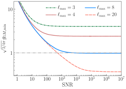
Figure 1: The smallest detectable (at the $3\sigma$ level) dipole-anisotropy coefficient $g_{1M}$ (multiplied by $\sqrt{3/4\pi}$). Results are shown as a function of the signal-to-noise ratio for the isotropic GW signal and for several values of the maximum timing-residual multipole moment $\ell_{\rm max}$ (which is $\ell_{\rm max}\simeq\sqrt{N_{p}}$ in terms of the number $N_{p}$ of pulsars).

We then set $\ell_{\rm max}\simeq N_{p}^{1/2}$, where $N_{p}$ is the number of pulsars, if these pulsars are distributed roughly uniformly on the sky; the sensitivity to higher-$\ell$ modes will be exponentially reduced. We then plot in Fig. 1 the smallest detectable (at the $\gtrsim 3\sigma$ confidence level) dipole-anisotropy amplitude $g_{1M}$ as a function of the signal-to-noise ratio SNR with which the isotropic signal is detected and for different numbers of pulsars. The results can be understood by noting that Eq. (31) becomes, in the ${\mathrm{SNR}}\to\infty$ limit and in the limit $\ell_{\rm max}\gg 1$,

$$g_{1M,{\rm min}}\sim\frac{6\sqrt{2\pi}}{\ell_{\rm max}},\qquad{\rm as}\,~{}{\mathrm{SNR}}\to\infty.$$ (32)

However, this asymptotic limit is reached only for very large SNR, given the very rapid decrease of $C_{\ell}/N^{zz}$ with $\ell$. In more physical terms, the anisotropy is inferred through correlations between spherical-harmonic modes of different $\ell$, and so individual modes of higher $\ell$ must be measured with high signal-to-noise. The steep dropoff of $C_{\ell}$ with $\ell$ (each of the seven $\ell=3$ moments has a signal-to-noise that is smaller by a factor of 5 than that for each quadrupole moment) requires that the isotropic signal (which is very heavily dominated by the quadrupole) be detected with very high significance. In the low-SNR limit, Eq. (31) is approximated,

$$g_{1M,{\rm min}}\sim\frac{28}{{\mathrm{SNR}}},\qquad{\rm as}\,~{}{\mathrm{SNR}}\to 0;$$ (33)

given the rapid decrease of the summand with $\ell$ in this low-SNR limit, this result is obtained for any $\ell_{\rm max}\geq 3$. In practice, this ${\mathrm{SNR}}\to 0$ limit is somewhat academic (and optimistic), as the factor $C_{\ell=2}/N^{zz}$ in the denominator of the summand in Eq. (31) is already 1.8 for ${\mathrm{SNR}}=3$. Thus, the numerical result is a bit larger, even for ${\mathrm{SNR}}=3$, than indicated by Eq. (33). The numerical results in Fig. 1 then indicate that the scaling with higher SNR is more like $({\mathrm{SNR}})^{-1/2}$ rather than $({\mathrm{SNR}})^{-1}$ at higher SNR, and that the ${\mathrm{SNR}}\to\infty$ limit (the “pulsar-number–limited regime”) is achieved for ${{\mathrm{SNR}}}\gtrsim 1000$. This can be understood by noting that, for example, the $C_{\ell}/N^{zz}$ in the denominator of the summand in Eq. (31) does not reach unity until the signal-to-noise ratio grows, for $\ell=4$, to ${\mathrm{SNR}}\gtrsim 60$, and for $\ell=8$, to ${\mathrm{SNR}}\gtrsim 1500$. This then shows that the benefit of $\gtrsim 16$ ($\gtrsim 64$) pulsars for this particular measurement is limited until the GW signal is detected at ${{\mathrm{SNR}}}\gtrsim 60$ ($\gtrsim 1500$).

If we wanted first to simply establish the existence of a dipole, without specifying its direction, then our observable would be the overall dipole amplitude,

$$d=\sqrt{\frac{3}{4\pi}}\left[\sum_{M}|g_{1M}|^{2}\right]^{1/2},$$ (34)

where we have included the factor of $\sqrt{4\pi}$ so that $d\leq 1$. The SNR with which this can be established is then $\sqrt{3}$ times that with which any individual $g_{1M}$ can be measured, and so the smallest detectable (at $3\sigma$) dipole has an amplitude

$$d_{\rm min} \simeq \frac{8}{{\mathrm{SNR}}},\qquad\mathrm{as}\ \ \ {\mathrm{SNR}}\to 0,$$

$$d_{\rm min} \simeq \frac{4}{\ell_{\rm max}},\qquad\mathrm{as}\ \ \ {\mathrm{SNR}}\to\infty,$$ (35)

again noting that the ${\mathrm{SNR}}\to 0$ limit is likely overly optimistic for ${\mathrm{SNR}}\gtrsim 3$ and the ${\mathrm{SNR}}\to\infty$ limit is valid for $\ell_{\rm max}\gg 1$.

VII.2 Higher $L$ modes

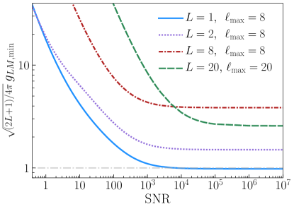
Figure 2: The smallest detectable anisotropy coefficient $g_{LM}$, for $L=\{1,2,8,20\}$, as a function of the total SNR with which the isotropic GW signal is detected. Results are provided for $\ell_{\rm max}=\{8,8,8,20\}$ respectively for the different $L$.

The results for higher $L$ of the smallest detectable $g_{LM}$ are easily obtained by numerical evaluation of Eq. (30) and shown for different $\ell_{\rm max}$ and (SNR) in Fig. 2. The qualitative dependence of the results are similar to those for $g_{1M,{\rm min}}$, although the sensitivity to higher-$L$ anisotropies is reduced a bit (e.g., by about 50% for $L=5$) relative to the dipole sensitivity.

VII.3 A gravitational-wave beam

Suppose that a gravitational-wave signal has been detected and that we wish to determine the fraction of the local gravitational-wave energy density coming from a specific direction. To be more precise suppose that we model the gravitational-wave signal as an isotropic uncorrelated background plus a flux of gravitational waves all coming from some specific direction (e.g., the direction of some specific SMBH binary candidate), which we take to be in the $\hat{z}$ direction, that makes up a fraction $f$ of the local GW energy density. This situation is described by anisotropy coefficients $g_{LM}=\sqrt{4\pi}f\sqrt{2L+1}\delta_{M0}$. The minimum-variance estimator for the amplitude $f$ is then obtained by summing the minimum-variance estimators for $g_{L0}$ (scaled by $\sqrt{4\pi}$), with inverse-variance weighting. In Fig. 3, we plot the smallest $f$ using the results above for $g_{LM,{\rm min}}$ for $L\leq 8$, detectable with measurements of $g_{LM}$ up to $L=8$, as a function of SNR from a single map and find it approaches $f_{\rm min}\simeq 0.1$ in the ${\mathrm{SNR}}\gtrsim 1000$ regime. It may be possible, however, to improve the sensitivity to a specific gravitational-wave point source if the signal is characterized by more than the incoherent flux assumed here.

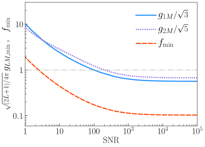
Figure 3: For $\ell_{\mathrm{max}}=8$, the smallest detectable dipole-anisotropy amplitude $d$ (which is $3^{-1/2}$ times the $g_{1M,\mathrm{min}}$ plotted in Fig. 1), and the smallest detectable quadrupole-anisotropy amplitude, shown together with the smallest detectable (again, at $3\sigma$) beam amplitude $f$ obtained with measurements of $g_{L0}$ up to L=8 is $f_{\mathrm{min}}\simeq 0.1$ in the high SNR limit.

VIII Multiple maps

So far, we have assumed that there is a single timing-residual map $z(\hat{n})$ obtained by convolving the time-domain data with a single window function. Suppose, however, that the time-domain data are convolved with $n_{w}$ different time-domain window functions that have negligible overlap in frequency space (or in phase). For example, if we were to have measurements performed, every two weeks for $\sim 10$ years, yielding $\sim 250$ measurements for each pulsar, the time-domain window functions could be taken to be the $\sim 250$ different time-domain Fourier modes. In this case, we will have $n_{w}\sim 250$ statistically independent timing-residual maps $z^{i}(\hat{n})$, with $i=1,2,\ldots,n_{w}$. If the Hellings-Downs power spectrum is detected with signal-to-noise ratio $({\mathrm{SNR}})_{i}$ in each individual map $i$, then the signal-to-noise ratio (squared) for the entire experiment, after co-adding all the information, will be $({\mathrm{SNR}})^{2}=\sum_{i}({\mathrm{SNR}})_{i}^{2}$.

The optimal estimator for any given $g_{LM}$ is then obtained by adding (with inverse-variance weighting) the estimators $\savestack{\tmpbox}{\stretchto{\scaleto{\scalerel*[\widthof{g_{LM}^{i}}]{\kern-0.6pt\bigwedge\kern-0.6pt}{\rule[-505.89pt]{4.30554pt}{505.89pt}}}{}}{0.5ex}}\stackon[1pt]{g_{LM}^{i}}{\tmpbox}$ from each map $i$; i.e., we augment Eq. (28) with an additional sum over $i$ and replace the SNR, the power spectrum $C_{\ell}$, and noise power spectrum $N^{zz}$ by those—$({\mathrm{SNR}})_{i}$, $C_{\ell}^{i}$, and $N_{i}^{zz}$—associated with the $i$th map:

$$(\Delta g_{LM})^{-2}=\frac{27}{16\pi^{3}}\sum_{i}\sum_{\ell\ell^{\prime}}\frac{(H^{L}_{\ell\ell^{\prime}}z_{\ell}z_{\ell^{\prime}}({\mathrm{SNR}})_{i}N_{i}^{zz})^{2}}{(C_{\ell}^{i}+N_{i}^{zz})(C_{\ell^{\prime}}^{i}+N_{i}^{zz})}.$$ (36)

The SNR, power spectrum, and noise power spectrum for each map are related by

$$C^{i}_{\ell}=\frac{3}{\pi}\sqrt{\frac{3}{2}}\frac{z_{\ell}^{2}}{2\ell+1}N^{zz}_{i}({\mathrm{SNR}})_{i},$$ (37)

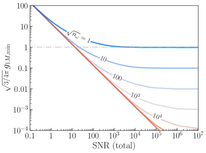
Figure 4: The smallest detectable dipole coefficient $g_{1M,{\rm min}}$ as a function of the total signal-to-noise for $\ell_{\rm max}=8$. The different curves show results obtained for different numbers of statistically independent maps $n_{\omega}$, assuming that the total SNR is distributed equally among all these maps.

In the ${\mathrm{SNR}}\to 0$ limit, these replacements result (given $\sum_{i}({\mathrm{SNR}})_{i}^{2}=({\mathrm{SNR}})^{2}$) in the same anisotropy sensitivity as inferred for a single map in this limit in Eq. (33). If, however, the signal-to-noise ratio ${\mathrm{SNR}}_{i}$ in some number $n_{\rm high}$ of maps is high enough (e.g., $({\mathrm{SNR}})_{i}\gtrsim 60$ for $N_{p}=16$ or $({\mathrm{SNR}})_{i}\gtrsim 1500$ for $N_{p}=64$) that pulsar-number–limited regime is reached in each individual map, then the sensitivity to anisotropy can be improved by a factor $\sqrt{n_{\rm high}}$ relative to that, Eq. (32), as shown in Fig. 4. It must be kept in mind that the improvement shown in Fig. 4 possible with additional maps is achieved only if the total SNR is split evenly among all of these many maps.

The remaining question, then, is how the total signal-to-noise is distributed among the maps. In the best-case scenario, it will be distributed equally among the $n_{w}$ maps. If so, then sensitivity to anisotropy could be improved, in principle, by the factor $\sqrt{n_{w}}$ over that in Eq. (32), as shown in Fig. 4. This improvement would require, however, that the total signal-to-noise be $\sim\sqrt{n_{w}}$ larger than that (${\mathrm{SNR}}\gtrsim 60$ for $N_{p}=16$ and ${\mathrm{SNR}}\gtrsim 1500$ for $N_{p}\gtrsim 64$) for a single map.

Given the likely (given the most promising astrophysical scenarios) decrease of the signal with GW frequency, however, the signal-to-noise will probably be dominated by a small subset of the maps (those at the lowest frequencies). If so, then $n_{\rm high}$ may be far smaller than $n_{w}$, and the sensitivity, from multiple maps, to anisotropy will be only marginally improved over the single-map estimate in Eq. (32).

IX Discussion

We have discussed the search for anisotropy in a PTA-detected gravitational-wave signal in terms of bipolar spherical harmonics for idealized measurements parametrized in terms of the number of pulsars (assumed to be uniformly distributed on the sky) and the signal-to-noise ratio (SNR) with which the isotropic signal is established. We focussed our attention first on the case of a single timing-residual map $z(\hat{n})$ (obtained from the convolution of the data with a single time-domain window function) and then discussed the generalization to multiple maps (which take into account more of the time-domain information).

We considered a search for anisotropy in an uncorrelated and unpolarized GW background in which the anisotropy is independent of GW frequency. In this case, the anisotropy is parametrized entirely in terms of spherical-harmonic coefficients $g_{LM}$. We derived the optimal estimators for these $g_{LM}$ for idealized measurements in which $N_{p}$ pulsars are distributed roughly uniformly on the sky and the same timing-residual noise in each pulsar. We then obtain the variance with which each $g_{LM}$ can be determined; this variance is expressed in terms of the signal-to-noise with which the isotropic signal is detected and in terms of the number of pulsars.

The main qualitative upshot of the analysis is that the isotropic signal will have to be established very well before there is any possibility to detect anisotropy. The reason stems from the the fact that the anisotropy is obtained (for odd $L$) through cross-correlation of spherical-harmonic modes $z_{\ell m}$ of the timing-residual map of different $\ell$ and from the fact (inferred from Eq. (24)) that $94\%$ of the $({\mathrm{SNR}})^{2}$ for the isotropic signal comes from $\ell=2$, with only $6\%$ coming from higher modes. Our numerical results in Fig. 1 show that with a single map it will require the isotropic signal to be established with ${\mathrm{SNR}}\gtrsim 1000$ before even the maximal dipole anisotropy can be distinguished, at the $3\sigma$ level, from a statistically isotropic background. This would, moreover, require $\gtrsim 60$ pulsars spread uniformly over the sky. The sensitivity to a dipole signal can be improved with more pulsars and/or (as Fig. 4 shows) with multiple maps, constructed with different statistically-independent time-domain window functions. This latter improvement can be achieved, however, only if the signal-to-noise is spread evenly among these different maps. Fig. 2 indicate the additional challenge facing a search for higher-order anisotropy.

When discussing the prospects to detect anisotropy, we must be careful to state clearly the question we are trying to answer. Here we have focused on the sensitivity to departures from statistical isotropy parametrized in terms of spherical-harmonic coefficients $g_{LM}$, under the null hypothesis of a statistically-isotropic background. This sensitivity is limited not only by measurement noise, but also by cosmic variance. In our null hypothesis of a statistically isotropic signal, the spherical-harmonic coefficients $z_{\ell m}$ for the map are selected, in the limit of no-noise measurements, from a distribution with variance $C_{\ell}$. Departures from statistical isotropy show up, roughly speaking, in terms of disparities between the amplitudes of the different $m$ modes for a given $\ell$. The conclusion of our analysis is that this is difficult to establish given the variance $C_{\ell}$ under the null hypothesis.

A measurement that is consistent with statistical isotropy may still well exhibit some evidence that the local GW background is a realization that exhibits anisotropy. Suppose, for example, that we had precise measurement of the five timing-residual quadrupole moments $z_{2m}$ and found that the $z_{22}$ and $z_{2,-2}$ components were significantly larger than the other three quadrupole moments. Our calculation [obtained by evaluating Eq. (30) with only the $\ell=\ell^{\prime}=2$ term] indicates that it would be impossible to infer from this measurement any departure from statistical isotropy. Still, if such a result were observed, it would indicate that the local GW signal is coming primarily from the $\pm\hat{z}$ direction. If there was indeed a strong candidate GW source (e.g., a SMBH-binary candidate) in the $\hat{z}$ direction, then this observation would provide some evidence that the GW signal was coming predominantly from that source.

Our initial calculations explored the detectability of anisotropy from a single timing-residual map obtained by convolving the data with a single time-domain window function. If, however, multiple maps that explore different GW frequency ranges can be obtained, then there are prospects to co-add the anisotropy estimators from those maps to improve upon the pulsar-number limit that arises from a single map. Significant improvement in this way requires, however, that the $z_{\ell m}$ are measured with high SNR in multiple maps.

We also considered the prospects to measure the fraction $f$ of the local GW intensity that comes from a given direction. We conclude also that measurement of $f$ will be similarly challenging: For example, we found a value $f_{\rm min}\simeq 0.1$ for the smallest detectable fraction for a survey with $64$ pulsars with ${\mathrm{SNR}}\gtrsim 1000$ for the isotropic signal. This calculation leaves out ingredients (e.g., timing, polarization, and source evolution) that, if included in the analysis, might improve the ability to localize a point source. Still, the rough conclusions and scalings of the sensitivities with SNR and pulsar number should translate to those for a more complete point-source search.

We also note, for possible comparison with previous work in configuration space Anholm:2008wy ; Mingarelli:2013dsa ; Gair:2014rwa , that a sky described by BiPoSHs $A^{LM}_{\ell\ell^{\prime}}$ has a two-point correlation function,

$$C(\hat{n},\hat{m})=C(\Theta)+\sum_{\ell\ell^{\prime}LM}\,A^{LM}_{\ell\ell^{\prime}}\,\,\{Y_{\ell}(\hat{n})\otimes Y_{\ell^{\prime}}(\hat{m})\}_{LM},$$ (38)

where

$$\{Y_{\ell}(\hat{n})\otimes Y_{\ell^{\prime}}(\hat{m})\}_{LM}=\sum_{mm^{\prime}}\langle\ell\,m\,\ell^{\prime}\,m^{\prime}|LM\rangle\,Y_{\ell m}(\hat{n})Y_{\ell^{\prime}m^{\prime}}(\hat{m}),$$ (39)

are the bipolar spherical harmonics (BipoSHs). These BiPoSHs constitute a complete orthonormal basis for functions of $\hat{n}$ and $\hat{m}$ in terms of total-angular-momentum states labeled by quantum numbers $L$ and $M$ composed of angular momentum states with $l$ and $l^{\prime}$; they are an alternative to the outer product of the $\{l,m\}$ and $\{l^{\prime},m^{\prime}\}$ bases. It should be possible to identify these bipolar spherical harmonics to the anisotropic correlation functions worked out in Refs. (Mingarelli:2013dsa, ; Gair:2014rwa, ; Taylor:2015udp, ), but we leave this exercise to future work.

The analysis presented here should be straightforwardly generalized to astrometric GW searches. As shown in Ref. Qin:2018yhy , the E-mode map from an astrometry survey provides the same information as a timing-residual map. Therefore, everything said here about a timing-residual map can be applied equally to the E-mode map. The higher density of stellar astrometric sources on the sky may ultimately allow higher $\ell_{\rm max}$ but the advantage of this higher $\ell_{\rm max}$ for anisotropy searches can be capitalized upon only with a sufficiently high SNR. The B modes in the astrometry map can provide additional statistically independent information and, when combined with the E modes and/or timing residuals, can conceivably improve the sensitivity to anisotropy by a factor of $\sqrt{2}$.

The numerical results we find for the sensitivity to anisotropy may be optimistic, given the idealizations assumed here. Uneven distribution of pulsars on the sky and/or pulsar-to-pulsar variations in the timing-residual noises will degrade the sensitivity. There is another, more subtle, caveat: The estimator in Eq. (27), and the expression, Eq. (28), for its variance, are derived under the assumption that the different $\savestack{\tmpbox}{\stretchto{\scaleto{\scalerel*[\widthof{A^{LM}_{\ell\ell^{\prime}}}]{\kern-0.6pt\bigwedge\kern-0.6pt}{\rule[-505.89pt]{4.30554pt}{505.89pt}}}{}}{0.5ex}}\stackon[1pt]{A^{LM}_{\ell\ell^{\prime}}}{\tmpbox}$ are statistically independent. Although the covariance between any two different $\savestack{\tmpbox}{\stretchto{\scaleto{\scalerel*[\widthof{A^{LM}_{\ell\ell^{\prime}}}]{\kern-0.6pt\bigwedge\kern-0.6pt}{\rule[-505.89pt]{4.30554pt}{505.89pt}}}{}}{0.5ex}}\stackon[1pt]{A^{LM}_{\ell\ell^{\prime}}}{\tmpbox}$ vanishes (except for those with $\ell\leftrightarrow\ell^{\prime}$), they are not statistically independent. The variance will thus most generally be a bit larger, and the sensitivity to anisotropy a bit degraded. We anticipate, though, that for the low-$L$ values considered here that this will be a relatively small (perhaps $\sim 10\%$) effect, although this should be evaluated further with Monte Carlo simulations of isotropic GW signals.

We hope that the approach developed here provides a conceptually straightforward way to understand the search for anisotropy in the GW background and aids in the development of observational/analysis strategies for the PTA search for gravitational waves. It will be interesting in future work to compare the results here to those obtained from detailed simulations of the PTA analysis pipeline, as well as with those inferred from a fully Bayesian approach (see similar applications for the cosmic microwave background Das:2015gca ; Shaikh:2019dvb , for example). It will also be interesing to extend the analysis here to seek anisotropies in the polarization of the GW background, as parametrized, for example, by GW Stokes parameters Conneely:2018wis , or anisotropies in the frequency dependence of the GW background. In the former work, authors compare the statistics of the GW Stokes parameters (spin 4) and concentrate on the isotropic spectra and cross-spectra, similar to this work, which builds a bridge between the two formalisms in terms of the statistical anisotropy of the amplitude fields that, as mentioned above, is a generalization of the power anisotropy.

In this paper we have considered ideal measurements in which GW-induced redshifts are measured as a function of position on the sky (with uniform sensitivity over the entire sky) and as a function of time (with uniform sampling/sensitivity). In this case, the harmonic-space basis is a cross product of spherical harmonics (for the sky) and Fourier modes for the time domain. In this idealized case, each (spherical-harmonic)–(time-domain Fourier mode) is statistically independent, for the GW background we are considering (i.e., that specified in Eq. (LABEL:eqn:generalized)). In practice, incomplete/irregular sky coverage, nonuniform timing-residual noise, and irregularities in the observation times destroy this elegant diagonalization. Techniques have been developed to deal with the cross-correlations induced by these imperfections on the idealized eigenmodes. For example, one can deal with real-space correlations, as done in prior work (e.g., Refs. (Mingarelli:2013dsa, ; Gair:2014rwa, ; Taylor:2015udp, )). Another option is to work with experiment-specific signal-to-noise eigenmodes (e.g., as being developed in Ref. (TCY:2019, )). Most generally, these imperfections will reduce the sensitivity to isotropic signals and/or anisotropy in the signal relative to those obtained here, assuming ideal measurements, although more detailed specification of the experiment is required to evaluate precisely the reduction in sensitivity.

During the preparation of this work, we learned of related work TCY:2019 in preparation that addresses prospects to detect anisotropy with a focus on developing a formalism to produce maps of the gravitational wave background from pulsar timing array measurements. We plan to follow up with detailed comparison of that work and the formalism described here.

X Erratum

In the original version of this paper, the equality $g_{LM}=\sqrt{4\pi}f\sqrt{2L+1}\delta_{M0}$ was missing the factor $2L+1$ on the right hand side. We thank Yacine Ali-Haïmoud, Tristan Smith and Chiara Mingarelli for spotting this error. As a result, the orange dashed curve in Fig. 3 was reduced by a factor of $\sim 2$ and our estimates for the $f_{\rm min}$ changed from $0.28$ to $0.1$ in the high SNR limit.

References

- (1) R. S. Foster and D. C. Backer, “Constructing a pulsar timing array,” Astrophys. J. 361, 300 (1990).
- (2) M. Maggiore, “Gravitational wave experiments and early universe cosmology,” Phys. Rept. 331, 283 (2000) [gr-qc/9909001].
- (3) S. Burke-Spolaor, “Gravitational-Wave Detection and Astrophysics with Pulsar Timing Arrays,” arXiv:1511.07869 [astro-ph.IM].
- (4) A. N. Lommen, “Pulsar timing arrays: the promise of gravitational wave detection,” Rept. Prog. Phys. 78, no. 12, 124901 (2015).
- (5) G. Hobbs and S. Dai, “A review of pulsar timing array gravitational wave research,” arXiv:1707.01615 [astro-ph.IM].
- (6) N. Yunes and X. Siemens, “Gravitational-Wave Tests of General Relativity with Ground-Based Detectors and Pulsar Timing-Arrays,” Living Rev. Rel. 16, 9 (2013) [arXiv:1304.3473 [gr-qc]].
- (7) G. Hobbs, “The Parkes Pulsar Timing Array,” Class. Quant. Grav. 30, 224007 (2013) [arXiv:1307.2629 [astro-ph.IM]].
- (8) R. N. Manchester et al., “The Parkes Pulsar Timing Array Project,” Publ. Astron. Soc. Austral. 30, 17 (2013) [arXiv:1210.6130 [astro-ph.IM]].
- (9) Z. Arzoumanian et al. [NANOGRAV Collaboration], “The NANOGrav 11-year Data Set: Pulsar-timing Constraints On The Stochastic Gravitational-wave Background,” Astrophys. J. 859, no. 1, 47 (2018) [arXiv:1801.02617 [astro-ph.HE]].
- (10) L. Lentati et al., “European Pulsar Timing Array Limits On An Isotropic Stochastic Gravitational-Wave Background,” Mon. Not. Roy. Astron. Soc. 453, no. 3, 2576 (2015) [arXiv:1504.03692 [astro-ph.CO]].
- (11) J. P. W. Verbiest et al., “The International Pulsar Timing Array: First Data Release,” Mon. Not. Roy. Astron. Soc. 458, no. 2, 1267 (2016) [arXiv:1602.03640 [astro-ph.IM]].
- (12) S. L. Detweiler, “Pulsar timing measurements and the search for gravitational waves,” Astrophys. J. 234, 1100 (1979).
- (13) M. V. Sazhin, “Opportunities for detecting ultralong gravitational waves,” Sov. Astron. 22, 36 (1978).
- (14) R. W. Hellings and G. S. Downs, “Upper Limits On The Isotropic Gravitational Radiation Background From Pulsar Timing Analysis,” Astrophys. J. 265, L39 (1983).
- (15) M. Rajagopal and R. W. Romani, “Ultralow frequency gravitational radiation from massive black hole binaries,” Astrophys. J. 446, 543 (1995) [astro-ph/9412038].
- (16) A. H. Jaffe and D. C. Backer, “Gravitational waves probe the coalescence rate of massive black hole binaries,” Astrophys. J. 583, 616 (2003) [astro-ph/0210148].
- (17) L. G. Book and E. E. Flanagan, “Astrometric Effects of a Stochastic Gravitational Wave Background,” Phys. Rev. D 83, 024024 (2011) [arXiv:1009.4192 [astro-ph.CO]].
- (18) C. J. Moore, D. Mihaylov, A. Lasenby and G. Gilmore, “Astrometric Search Method for Individually Resolvable Gravitational Wave Sources with Gaia,” Phys. Rev. Lett. 119, no. 26, 261102 (2017) [arXiv:1707.06239 [astro-ph.IM]].
- (19) D. P. Mihaylov, C. J. Moore, J. R. Gair, A. Lasenby and G. Gilmore, “Astrometric Effects of Gravitational Wave Backgrounds with non-Einsteinian Polarizations,” Phys. Rev. D 97, no. 12, 124058 (2018) [arXiv:1804.00660 [gr-qc]].
- (20) L. O’Beirne and N. J. Cornish, “Constraining the Polarization Content of Gravitational Waves with Astrometry,” Phys. Rev. D 98, no. 2, 024020 (2018) [arXiv:1804.03146 [gr-qc]].
- (21) W. Qin, K. K. Boddy, M. Kamionkowski and L. Dai, “Pulsar-timing arrays, astrometry, and gravitational waves,” Phys. Rev. D 99, no. 6, 063002 (2019) [arXiv:1810.02369 [astro-ph.CO]].
- (22) B. Allen and A. C. Ottewill, “Detection of anisotropies in the gravitational wave stochastic background,” Phys. Rev. D 56, 545 (1997) [gr-qc/9607068].
- (23) A. Sesana, A. Vecchio and M. Volonteri, Mon. Not. Roy. Astron. Soc. 394, 2255 (2009) doi:10.1111/j.1365-2966.2009.14499.x [arXiv:0809.3412 [astro-ph]].
- (24) V. Ravi, J. S. B. Wyithe, G. Hobbs, R. M. Shannon, R. N. Manchester, D. R. B. Yardley and M. J. Keith, “Does a ’stochastic’ background of gravitational waves exist in the pulsar timing band?,” Astrophys. J. 761, 84 (2012) [arXiv:1210.3854 [astro-ph.CO]].
- (25) N. J. Cornish and A. Sesana, “Pulsar Timing Array Analysis for Black Hole Backgrounds,” Class. Quant. Grav. 30, 224005 (2013) [arXiv:1305.0326 [gr-qc]].
- (26) L. Z. Kelley, L. Blecha, L. Hernquist, A. Sesana and S. R. Taylor, “Single Sources in the Low-Frequency Gravitational Wave Sky: properties and time to detection by pulsar timing arrays,” Mon. Not. Roy. Astron. Soc. 477, no. 1, 964 (2018) [arXiv:1711.00075 [astro-ph.HE]].
- (27) S. Kuroyanagi, K. Takahashi, N. Yonemaru and H. Kumamoto, “Anisotropies in the gravitational wave background as a probe of the cosmic string network,” Phys. Rev. D 95, no. 4, 043531 (2017) [arXiv:1604.00332 [astro-ph.CO]].
- (28) M. Anholm, S. Ballmer, J. D. E. Creighton, L. R. Price and X. Siemens, “Optimal strategies for gravitational wave stochastic background searches in pulsar timing data,” Phys. Rev. D 79, 084030 (2009) [arXiv:0809.0701 [gr-qc]].
- (29) C. M. F. Mingarelli, T. Sidery, I. Mandel and A. Vecchio, “Characterizing gravitational wave stochastic background anisotropy with pulsar timing arrays,” Phys. Rev. D 88, no. 6, 062005 (2013) [arXiv:1306.5394 [astro-ph.HE]].
- (30) J. Gair, J. D. Romano, S. Taylor and C. M. F. Mingarelli, “Mapping gravitational-wave backgrounds using methods from CMB analysis: Application to pulsar timing arrays,” Phys. Rev. D 90, no. 8, 082001 (2014) [arXiv:1406.4664 [gr-qc]].
- (31) S. R. Taylor et al., “Limits on anisotropy in the nanohertz stochastic gravitational-wave background,” Phys. Rev. Lett. 115, no. 4, 041101 (2015) [arXiv:1506.08817 [astro-ph.HE]].
- (32) A. Hajian and T. Souradeep, “Measuring statistical isotropy of the CMB anisotropy,” Astrophys. J. 597, L5 (2003) [astro-ph/0308001].
- (33) A. Hajian and T. Souradeep, “The Cosmic microwave background bipolar power spectrum: Basic formalism and applications,” astro-ph/0501001.
- (34) N. Joshi, S. Jhingan, T. Souradeep and A. Hajian, “Bipolar Harmonic encoding of CMB correlation patterns,” Phys. Rev. D 81, 083012 (2010) [arXiv:0912.3217 [astro-ph.CO]].
- (35) E. Roebber and G. Holder, “Harmonic space analysis of pulsar timing array redshift maps,” Astrophys. J. 835, no. 1, 21 (2017) [arXiv:1609.06758 [astro-ph.CO]].
- (36) L. G. Book, M. Kamionkowski and T. Souradeep, “Odd-Parity Bipolar Spherical Harmonics,” Phys. Rev. D 85, 023010 (2012) [arXiv:1109.2910 [astro-ph.CO]].
- (37) A. R. Pullen and M. Kamionkowski, “Cosmic Microwave Background Statistics for a Direction-Dependent Primordial Power Spectrum,” Phys. Rev. D 76, 103529 (2007) [arXiv:0709.1144 [astro-ph]].
- (38) S. Das, B. D. Wandelt and T. Souradeep, JCAP 1510, no. 10, 050 (2015) doi:10.1088/1475-7516/2015/10/050 [arXiv:1509.07137 [astro-ph.CO]].
- (39) S. Shaikh, S. Mukherjee, S. Das, B. D. Wandelt and T. Souradeep, arXiv:1902.10155 [astro-ph.CO].
- (40) C. Conneely, A. H. Jaffe and C. M. F. Mingarelli, “On the Amplitude and Stokes Parameters of a Stochastic Gravitational-Wave Background,” arXiv:1808.05920 [astro-ph.CO].
- (41) T. L. Smith, Y. Ali-Haïmoud, and C. M. F. Mingarelli, in preparation.