Cross-Platform Performance Portability Using Highly Parametrized SYCL Kernels

Abstract.

Over recent years heterogeneous systems have become more prevalent across HPC systems, with over 100 supercomputers in the TOP500 incorporating GPUs or other accelerators. These hardware platforms have different performance characteristics and optimization requirements. In order to make the most of multiple accelerators a developer has to provide implementations of their algorithms tuned for each device. Hardware vendors provide libraries targeting their devices specifically, which provide good performance but frequently have different API designs, hampering portability.

The SYCL programming model allows users to write heterogeneous programs using completely standard C++, and so developers have access to the power of C++ templates when developing compute kernels. In this paper we show that by writing highly parameterized kernels for matrix multiplies and convolutions we achieve performance competitive with vendor implementations across different architectures. Furthermore, tuning for new devices amounts to choosing the combinations of kernel parameters that perform best on the hardware.

1. Introduction

The power and speed of modern GPUs coupled with their increased programmability through programming models such as SYCL (syc, [n. d.]b), OpenCL (Stone et al., 2010) and CUDA (cud, [n. d.]) have enabled many applications to achieve previously insurmountable performance. This has been one of the main driving factors behind the rise in machine learning since 2012. In the TOP500 (top, [n. d.]), 3 of the top 5 supercomputers in the world in terms of pure performance utilize GPUs, as do the top 4 supercomputers in the Green500 (gre, [n. d.]), where flops per watt are considered.

Many hardware vendors provide highly specialized libraries for their platforms to extract optimal performance from their hardware. As more companies and computing centers move to support larger heterogeneous systems with more varied hardware this means users have to write applications which handle multiple different libraries for each available accelerator. This adds complexity both for developers and system maintainers.

2. Related Works

Highly specialized libraries—such as ARM Compute Library (acl, [n. d.]), cuBLAS (nvi, [n. d.]a), cuDNN (Chetlur et al., 2014), CUTLASS (Kerr et al., [n. d.]), MIOpen (mio, [n. d.]), Intel MKL (Wang et al., 2014) and MKL-DNN (mkl, [n. d.])—provide optimal performance on the targeted hardware, however typically each of these libraries are restricted to the vendor’s hardware.

A common way of achieving performance across various platforms is to specialize certain routines in a library or framework targeting a particular architecture. There are various high performance vendor-specified libraries tuned for particular architectures.

For ARM devices, ARM Compute Library (acl, [n. d.]) provides a set of low-level, optimized primitives for machine-learning and linear algebra. While for NVIDIA devices, cuBLAS (nvi, [n. d.]a) and cuDNN (Chetlur et al., 2014) provide highly optimized implementations of standard linear algebra subroutines and deep neural network routines, respectively. NVIDIA also provides a higher level CUTLASS (Kerr et al., [n. d.]) which takes advantage of CUDA C++ templates meta programming to deliver a high-performance GEMM computations allowing developers to specialize their matrix multiplies inside their application.

Similarly AMD provides MIOpen (mio, [n. d.]), a deep learning acceleration framework developed to deliver highly optimized DNN and GEMM routines for AMD GPUs. For their multi-core and many-core systems, Intel provides MKL (Wang et al., 2014) for linear algebra routines, and MKL-DNN (mkl, [n. d.]) as an open source, high performance library for accelerating deep learning frameworks.

Each of these libraries are optimized specifically for their target devices, however do not provide performance portability. The limitations of these libraries highlight two main key factors in providing this: the parallel programming framework used to develop the library and the performance metrics of devices.

2.1. Parallel programming frameworks

There are many different frameworks available to provide access to hardware parallelism, with different approaches and programming styles. Most are based on C or C++, with variations on the language to allow a developer to specify how tasks can be parallelized.

The Intel Thread Building Blocks (TBB) library (Pheatt, 2008) is a C++ template library for parallel programming on multi-core processors. TBB only provides parallelism on CPUs so applications developed on top of TBB are not portable to GPU or accelerated platforms.

On the other hand, CUDA (cud, [n. d.]) is used by NVIDIA as a low level framework to deliver performance on NVIDA GPUs and accelerators, but not CPUs. Although CUDA C++ supports template metaprogramming features which is necessary for performance portability, the lack of CUDA support on non-NVIDIA architecture prevents more widespread adoption.

A cross-platform framework like OpenCL (Stone et al., 2010) can be supported by various vendors and platforms, however the low level interface of OpenCL hampers development of easily tunable kernels that enable performance portability. Although OpenCL 2.1 supports template metaprogramming within kernels, the kernel interface itself cannot be templated, which limits the use of this feature.

SYCL (syc, [n. d.]b; Reyes and Lomüller, 2015) is an open standard maintained by the Khronos Group, a collaboration of companies, universities and individuals dedicated to developing open standards, known for maintaining OpenCL, Vulkan, OpenGL and many others alongside SYCL. The standard is a royalty-free, cross-platform abstraction layer that enables developers to utilize heterogeneous systems with varied hardware while writing completely standard C++.

SYCL provides a highly parallel programming model designed to abstract away much of the complexity of traditional parallel programming models like OpenCL. Using SYCL instead of a lower level interface like OpenCL allows the developer to write code using modern C++ language features, even within their accelerated kernels. This includes the use of templates and specializations, as well as the metaprogramming that these enable, instead of the heavy use of the preprocessor typical in OpenCL applications to provide specializations within kernels for data types, tile sizes and other constants. By allowing SYCL kernels to fully utilize C++, a developer can instead use templates to provide these compile time constants, as well as easily create many specialized kernels with very little additional code.

Combining the portability of OpenCL with modern C++ template metaprogramming makes SYCL a strong parallel programming framework for performance portability across different platforms.

ComputeCpp (com, [n. d.]), developed by Codeplay Software, is currently the only fully conformant implementation of the SYCL standard, supporting devices from AMD, Intel, NVIDIA and others. Several open-source libraries are compatible with ComputeCpp, including SYCL-DNN (syc, [n. d.]c), VisionCpp (Goli, 2016; vis, [n. d.]), SYCL-PRNG (syc, [n. d.]d), as well as contributed parts of Eigen (Guennebaud et al., 2010; Goli, 2017) and TensorFlow (Abadi et al., 2015; Goli et al., 2017; Goli et al., 2018).

2.2. Performance Metrics

Tuning the performance of accelerated compute kernels is not a trivial task requiring expertise in both parallel algorithms and hardware architectures. Having said that, many hardware accelerators share common factors affecting performance, allowing common algorithmic techniques for improving performance across devices.

We have studied common hardware-related optimization improvements on the following devices: Intel CPUs and GPUs, ARM Mali GPUs, AMD GPUs and the Renesas V3H and V3M accelerators. These metrics are used to develop parametric convolution and matrix multiply algorithms, two of the most computationally intense operations used in neural networks.

2.2.1. Thread reusability

The number of individual compute units available in hardware varies significantly, from 2 in embedded systems to 84 in desktop GPUs e.g NVIDIA Tesla series. Depending on the number of compute units available the size of workload per thread can be parametrized in order to achieve maximal device occupancy. However, there is a trade off between increasing the number of work-groups and ensuring a sufficient workload per thread. For a given problem, creating more work groups or more threads will naturally decrease the amount of computation that any one thread will have to do.

2.2.2. Memory transactions

In most accelerators, when a set of threads within a work-group loads data, an entire block of data called a cache-line is fetched from memory. This is based on the assumption that threads within a work-group access contiguous elements of data specified in the fetched block. Assuming the threads within a work-group access the same address, the permutation, masking or prediction has no effect on the loaded block of data, which can lead to more optimizations in the compiler. Moreover loading a block of data will reduce the number of memory transactions, improving performance (nvi, [n. d.]b).

2.2.3. Data reusability

Memory accesses tend to be the bottleneck in GPU programming, despite graphics memory typically being much faster than standard DDR memory. As a result of this, many optimizations to GPU kernels involve maximizing data reuse to minimize the amount of data that needs to be fetched from memory. Hardware devices provide a memory hierarchy in order to reduce the memory access bottleneck which is categorized into global, local, and private memory regions in OpenCL terms, each of which can be controlled by programmers.

Common techniques to maximize data reusability include utilizing local memory as a programmable cache to allow a work group to reuse data loaded from global memory, and through using blocks of private memory to allow single threads to reuse memory. Private memory usually maps to hardware registers and so can be accessed incredibly quickly. Provided there are sufficient registers, the more we can re-use data located in registers, the better the performance.

Local memory access speeds are usually equivalent to caches. Nowadays many hardware vendors (e.g. Intel and ARM) provide large caches in front of their global memory and so can achieve similar performance to using programmer-controlled local memory when accessing data in a coalesced manner. Therefore, some embedded devices like ARM’s Mali G-71 GPU do not dedicate any memory for local memory, instead relying on the cache and global memory. For such devices using local memory can be costly and negatively affect performance.

Table 1. Performance metrics of various compute devices, as discussed in Section 2.2.

Device name	Cache line	Local memory	Compute units
Intel Core i7-6700K CPU	64 bytes	None	8
Intel Core i7-6700K GPU	64 bytes	64 KiB	24
ARM Mali G71 GPU	64 bytes	None	8
Renesas V3M	128 bytes	447 KiB	2
Renesas V3H	128 bytes	409 KiB	5
AMD R9 Nano	128 bytes	32 KiB	64

2.2.4. Vectorization

Many GPU architectures have memory controllers which are designed to load and store multiple elements at once, as typical graphics workloads involve 4-element vectors. To get the best performance from these load-store units, computations should make use of vector loads and stores. Another benefit of using vectors in a GPU kernel even if the hardware does not support vector computations is that each vector element can be computed separately, and so there is increased instruction level parallelism.

Table 1 summarizes the hardware features required for abstracting performance metrics for convolution and matrix multiply algorithms.

2.3. Research Niche

In this paper, we have designed and developed parametric algorithms for matrix multiplication and convolution—two of the most computationally intense operations in neural networks—which can be tuned according to the performance metrics of various devices. Written on top of SYCL, these implementations abstract common performance metrics, enabling performance portability across different platforms.

3. SYCL-BLAS

SYCL-BLAS (syc, [n. d.]a) is an open source implementation of netlib BLAS (bla, [n. d.]) which enables performance portability across a range of accelerators. SYCL-BLAS uses an expression tree design to deliver BLAS co-routines; most of the BLAS Level 1 and BLAS Level 2 co-routines are memory-bound operations so using such an expression tree based approach allows multiple operations to be fused into a single compute kernel with a higher computational complexity. Increasing the computational intensity of memory-bound applications can significantly increase the performance by reducing the number of accesses to the device’s global memory (Aliaga et al., 2017).

The general matrix multiply operation (GEMM) is the heart of BLAS routines, used in a wide range of scientific domains from physics to machine learning. It is one of the computationally expensive operation in neural networks, and so optimizing GEMM can improve a DNN’s performance.

3.1. GEMM

The General Matrix-Matrix product is a BLAS operation defined as:

$$C=\alpha\times\operatorname{OP}_{a}(A)\times\operatorname{OP}_{b}(B)+\beta\times C,$$

where $A$, $B$ and $C$ are column-major matrices, and $\operatorname{OP}_{a}$ and $\operatorname{OP}_{b}$ are either identity or transpose operators (or conjugate transpose for complex data types).

We refer to $M$ and $N$ as the number of rows and columns of $C$, respectively, and $K$ as the contracting dimension of $A$ and $B$. A naive parallelization approach on massively parallel architectures is to assign one value of the output $C$ per thread to accumulate the dot product of the $i$-th row of $\operatorname{OP}_{a}(A)$ with the $j$-th column of $\operatorname{OP}_{b}(B)$ in a local register $r$, and update the result: $C(i,j)=\alpha r+\beta C(i,j)$. However, this approach is highly memory-bounded as each thread is required to load $2\times k$ data elements while performing roughly $2\times k$ floating point operations.

A standard approach used to improve performance of dense linear algebra operations on modern hardware is to reduce the memory latency by increasing data reusability through a tiling technique (Gustavson et al., 1998; Nath et al., 2010).

3.1.1. Blocked GEMM

Given two matrices $A_{M\times K}$ and $B_{K\times N}$ and partitions

(1) $$\begin{split}0&=M_{0}<\dotsb<M_{m}=M\in[0,M]\\ 0&=K_{0}<\dotsb<K_{k}=K\in[0,K]\\ 0&=N_{0}<\dotsb<N_{n}=N\in[0,N]\end{split}$$

then the following holds:

$$(A\times B)(M_{i-1}:M_{i},N_{j-1}:N_{j})=\\ A\left(M_{i-1}:M_{i},K_{0}:K_{1}\right)\times B\left(K_{0}:K_{1},N_{j-1}:N_{j}\right)+\dotsb+\\ A\left(M_{i-1}:M_{i},K_{k-1}:K_{k}\right)\times B\left(K_{0}:K_{1},N_{j-1}:N_{j}\right)$$

Thus, block matrices can be multiplied in the same way as regular matrices, by replacing each scalar multiply with a matrix multiply, and each scalar addition with a matrix addition.

A special case of the above property allows us to partition matrices $A^{\prime}$ and $B^{\prime}$ into panels, and matrix $C$ into blocks where the partitioning of C dictates the partitioning of $A^{\prime}$ and $B^{\prime}$:

(2) $$A^{\prime} =\left[\begin{array}[]{c}A_{1}\\ \vdots\\ A_{M}\end{array}\right]$$

$$B^{\prime} =\left[\begin{array}[]{ccc}B_{1}&\dotsb&B_{N}\end{array}\right]$$

$$C =\left[\begin{array}[]{ccc}C_{11}&\dotsb&C_{1N}\\ \vdots&\ddots&\vdots\\ C_{M1}&\dotsb&C_{MN}\\ \end{array}\right]$$

Then each thread can compute a panel in the matrix multiply:

$$C_{ij}=\alpha\times A_{i}\times B_{j}+\beta\times C{ij}.$$

Each panel can then itself be broken down further into tiles and we recursively build tiles of smaller matrices in different memory hierarchies. To illustrate this tile based approach, suppose we are performing an $8\times 8$ floating point matrix multiply, for a device with 128 bytes of local memory and a maximum of 12 float registers available without spilling. Further suppose that 4 work-groups with 4 threads in each work-group are created. Figure 1(a) represents the $A^{\prime}$ and $B^{\prime}$ panels and $C$ blocks in global memory. The tile sizes are different in the memory hierarchies due to memory size limitations. The faster the memory is, the smaller the size of the memory, and therefore the smaller the tile size. Thus multiple iterations are required to load all the required data for the computation.

Since the total number of threads is 16, each thread computes 4 output elements. At first all threads of a work-group load the first tile of the $A^{\prime}$ and $B^{\prime}$ panel (the yellow square in Figure 1(a)) into local memory in a coalesced way. Given the size of the local memory, each input matrix must be broken into two tiles (represented by yellow and orange color in Figure 1(a)) where one tile per matrix can be loaded into local memory at once (Figure 1(b)). Similarly, each tile of the $A^{\prime}$ and $B^{\prime}$ panels in local memory is broken into 7 tiles of $A^{\prime\prime}$ and $B^{\prime\prime}$ to compute the matrix multiply without register spill (Figure 1(c) and Figure 1(d)).

Moreover, there are different ways of loading tiles from local memory to registers. Figure 1(c) loads the local memory tiles into 7 separate register tiles, which enables coalesced writes to global memory. In Figure 1(d), although the number of tiles is reduced due to using more registers, each thread writes a block of 2 consecutive elements, thus the memory writes are not coalesced.

Choosing between the two above tile configurations at the private memory level is platform specific. While in a SIMD platform coalesced read/write have a significant effect on performance, on non-SIMD devices (e.g CPUs) block data accesses and a reduced tile count provide better performance.

Providing a parametric GEMM enables a programmer to tune the operation for different platforms by choosing different configurations without re-implementing the kernel.

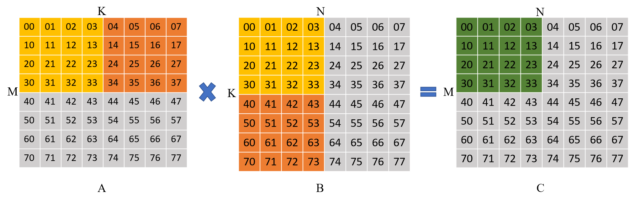
A matrix multiplication between two 8 by 8 matrices with the first 4 by 4 submatrix of the result highlighted, along with the corresponding panel of the first 4 rows of the left hand matrix and the first 4 columns of the right hand matrix which contribute to that output submatrix.

(a) global memory

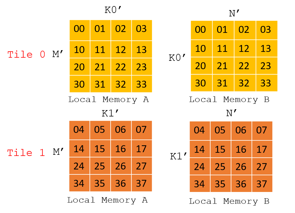
The highlighted panels from Figure 1(a) of the two input matrices split into 4 by 4 blocks, containing the data required to compute a 4 by 4 block of the output matrix.

(b) local memory

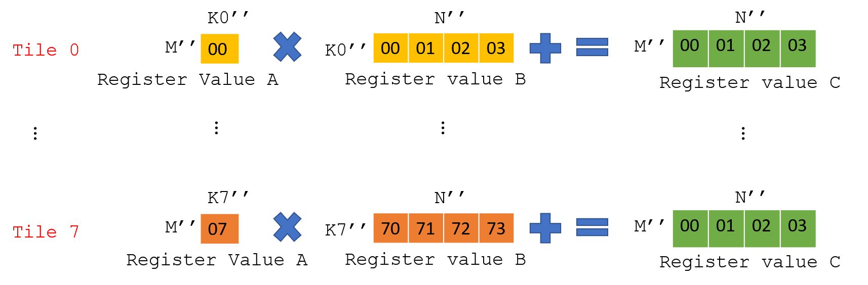
The blocks from Figure 1(b) split into individual registers, showing the computation of 4 elements of the output. The first 4 output elements depend on the first row of the left hand matrix and on the first 4 columns of the right hand matrix. When individual values of the left hand matrix are loaded one by one there are 8 vector multiply-adds.

(c) private memory

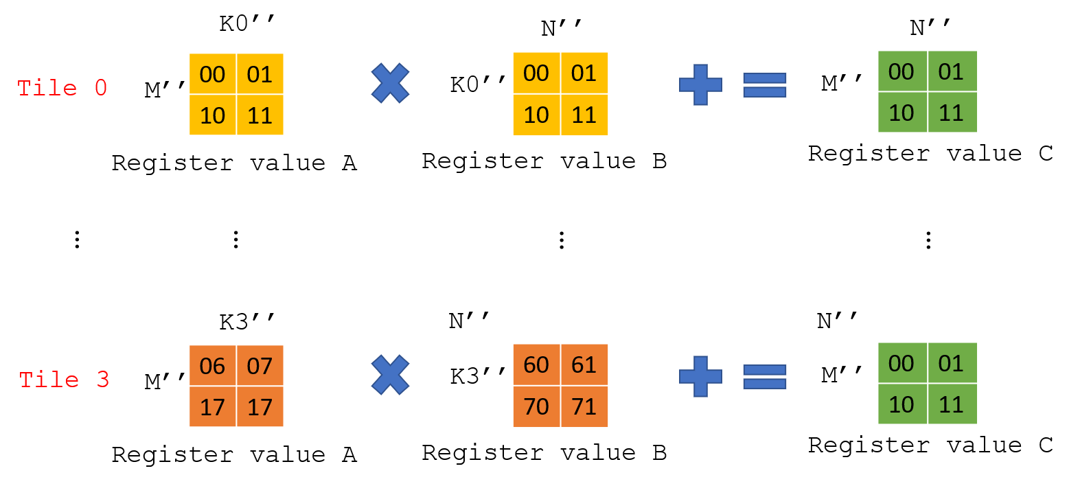
Similar to Figure 1(c), the block matrices are split into registers however here the left hand matrix is split into small 2 by 2 tiles in registers. This allows a 2 by 2 output tile to be computed over 4 tiles.

(d) private memory

Figure 1. Tiled-based Matrix multiply

3.1.2. Data reuse in a GEMM operation

Assuming a $m^{\prime}\times n^{\prime}$ submatrix $C_{ij}$ is already in registers, the computation of a single block across $k^{\prime}$ elements requires reading $m^{\prime}k^{\prime}+k^{\prime}n^{\prime}$ data entries from global memory, and requires $2m^{\prime}n^{\prime}k^{\prime}$ floating point operations.

Overall, $2Km^{\prime}n^{\prime}$ floating point operations are needed to compute $C_{ij}$, and $m^{\prime}n^{\prime}+m^{\prime}K+n^{\prime}K$ data elements are required to be loaded from global memory.

The panels $A_{i}$ and $B_{j}$ are read in blocks of size $k^{\prime}$, due to memory and register limitations. Then each block of $A_{i}$ will be multiplied with the appropriate block of $B_{j}$ and accumulated into $C_{ij}$. In this way $C_{ij}$ is stored in registers during the entire operation and only written to global memory at the end.

The amount of data reuse obtained through this tiled approach to multiplying blocks is therefore given by:

(3) $$\frac{2m^{\prime}n^{\prime}k^{\prime}}{m^{\prime}k^{\prime}+k^{\prime}n^{\prime}}=\frac{2m^{\prime}n^{\prime}}{m^{\prime}+n^{\prime}}.$$

Since the goal of the blocking is to improve the amount of data reuse, the block sizes should be chosen to maximize this property.

Equation 3 shows that increasing $k^{\prime}$ does not increase the amount of data reuse, but does increase the amount of register/local memory/cache space required to store the matrices. For the tiles in private memory $k^{\prime}=1$ seems to be the best choice. Increasing $m^{\prime}$ and $n^{\prime}$ increases data reusability, but it also increases the amount of local memory/register/cache space that is required. It can easily be shown that, with an upper limit on the available amount of memory, the best reuse is obtained if $m^{\prime}=n^{\prime}$, i.e. if blocks $C_{ij}$ are chosen to be square.

When supported, using local memory will significantly improve the performance when $A$ is transposed or $B$ is not transposed. The other two possibilities may not require explicit copies from global to local memory, as assigning items to elements of the block in the correct order yields a perfectly coalesced read of these matrices from memory. Such temporal locality ensures that the data is already cached when a different item of the same work group requests the same data entity. However, moving the data explicitly to local memory can improve performance when the hardware cache unit is a slower than the local memory unit.

Software pre-fetching or double buffering is a well-known technique to overcome the latency of off-chip memory accesses. By doubling the size of local memory, it is possible to load the next tile while computing the current tile. This can hide the latency of the loads by computations.

4. SYCL-DNN

SYCL-DNN (syc, [n. d.]c) is an open-source library which provides optimized routines to accelerate neural network operations. It is built using the SYCL programming model to enable cross platform support, and so works on any accelerator supported by the user’s chosen SYCL implementation.

Modern image recognition networks mainly involve many convolutions and matrix multiplies, which make up the majority of the runtime of these networks. The matrix multiplies can be supplied by a BLAS implementation like SYCL-BLAS. The purpose of SYCL-DNN is to provide convolutions and other similar routines which are required for these networks.

4.1. Convolutions

Convolutions are typically the most compute intensive operation in these networks, and so they are the most optimized in the library. To optimize this operation, SYCL-DNN provide implementations of a number of algorithms which compute a 2D convolution. These different algorithms have different performance characteristics and memory requirements, and so behave differently for different tensor sizes and on different devices.

In neural networks, a 2D convolution is an operation taking a batch of 3D input tensors and a 4D filter tensor. Each output element is the sum of products of an input value and a weight given by sliding a small window over the input tensor.

More formally, let $H$ be the number of rows in the input, $W$ the number of columns, $C$ the number of input channels, $K$ the number of output channels and $R\times S$ the filter size. Then the input tensor $I\in\mathbb{R}^{H\times W\times C}$ and the filter tensor $F\in\mathbb{R}^{R\times S\times C\times K}$ would give rise to an output tensor $O\in\mathbb{R}^{H\times W\times K}$.

Data: input[$H$][$W$][$C$]

Data: filter[$R$][$S$][$C$][$K$]

Data: output[$H$][$W$][$K$]

for h = 1 to $H$ do

      for w = 1 to $W$ do

            for k = 1 to $K$ do

                  out = 0

                   for x = 1 to $R$ do

                        for y = 1 to $S$ do

                              for c = 1 to $C$ do

                                    out += input[h + x][h + y][c] * filter[x][y][c][k]

                                    

                               end for

                              

                         end for

                        

                   end for

                  output[h][w][k] = out

                  

             end for

            

       end for

      

end for

Algorithm 1 Naive algorithm to compute 2D convolution.

Using these layouts, the convolution can be computed naively as described in Algorithm 1. For example with a filter size of 3 $\times$ 3, an output element at row $h$, column $w$ and channel $k$ would be computed as:

$$o_{h,w,k}=\sum_{c=1}^{C}\sum_{x=1}^{3}\sum_{y=1}^{3}i^{h,w}_{x,y,c}\times f_{x,y,c,k}$$

where $i^{h,w}$ is a $3\times 3\times C$ slice of the input tensor centered at row $h$ and column $w$.

4.1.1. Tiling 2D convolutions

For convolutions with window sizes greater than $1$, there are overlaps in the regions of the input tensor which affects two spatially adjacent output elements. The naive method of computing a convolution using Algorithm 1 on a GPU would use a single thread per output element, which means every thread has to load all of the input slice that it requires from memory.

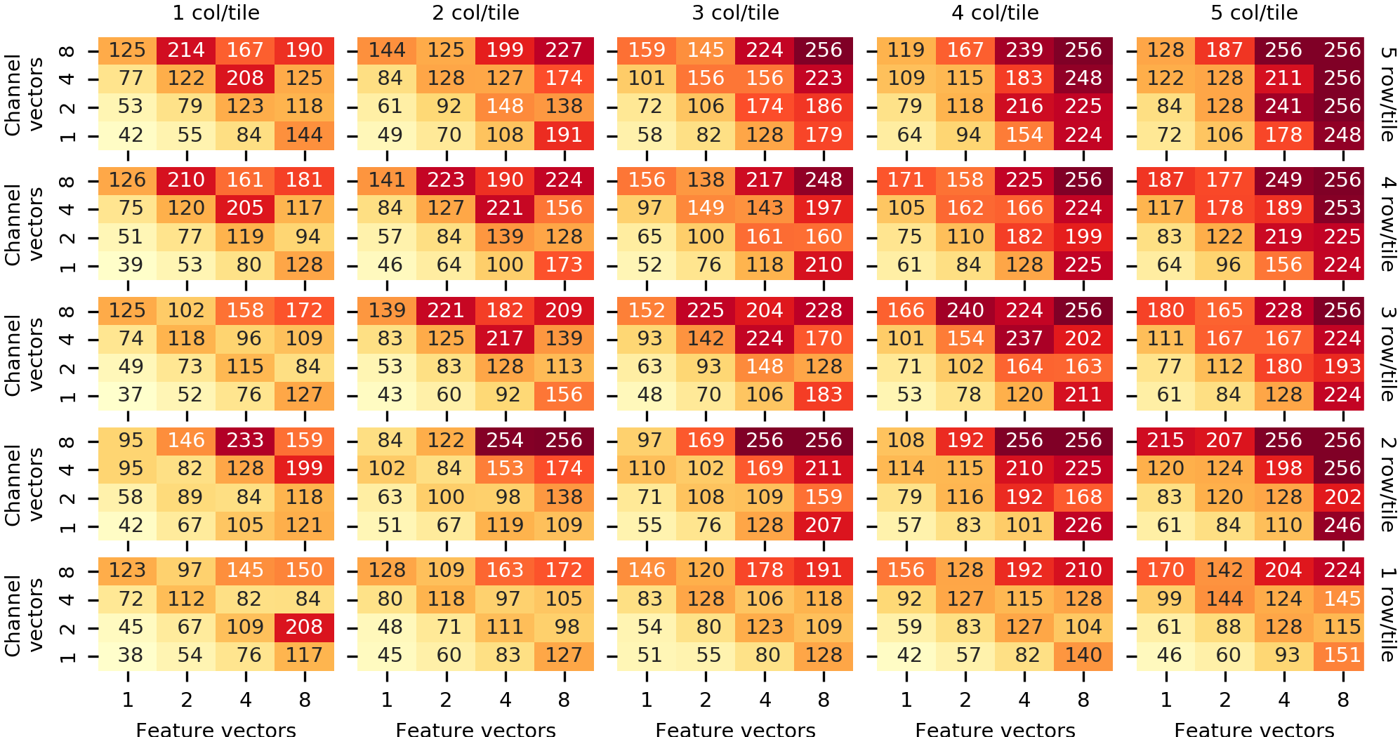
A grid of heatmaps where each heatmap corresponds to a given tile size, from 1 by 1 up to 5 by 5. Inside a given heatmap the entries are given by power of 2 vector sizes from 1 to 8. The number of registers increases as the tile increases and as the vector sizes increases from 38 registers in the naive case through to 256 in the largest tile sizes.

Figure 2. Number of registers used for different tile sizes and vector sizes for SYCL-DNN’s tiled 3$\times$3 convolution kernel. Each subplot gives the number of registers used for a given tile size as the vector sizes vary. Register usage data generated by AMD CodeXL (cod, [n. d.]).

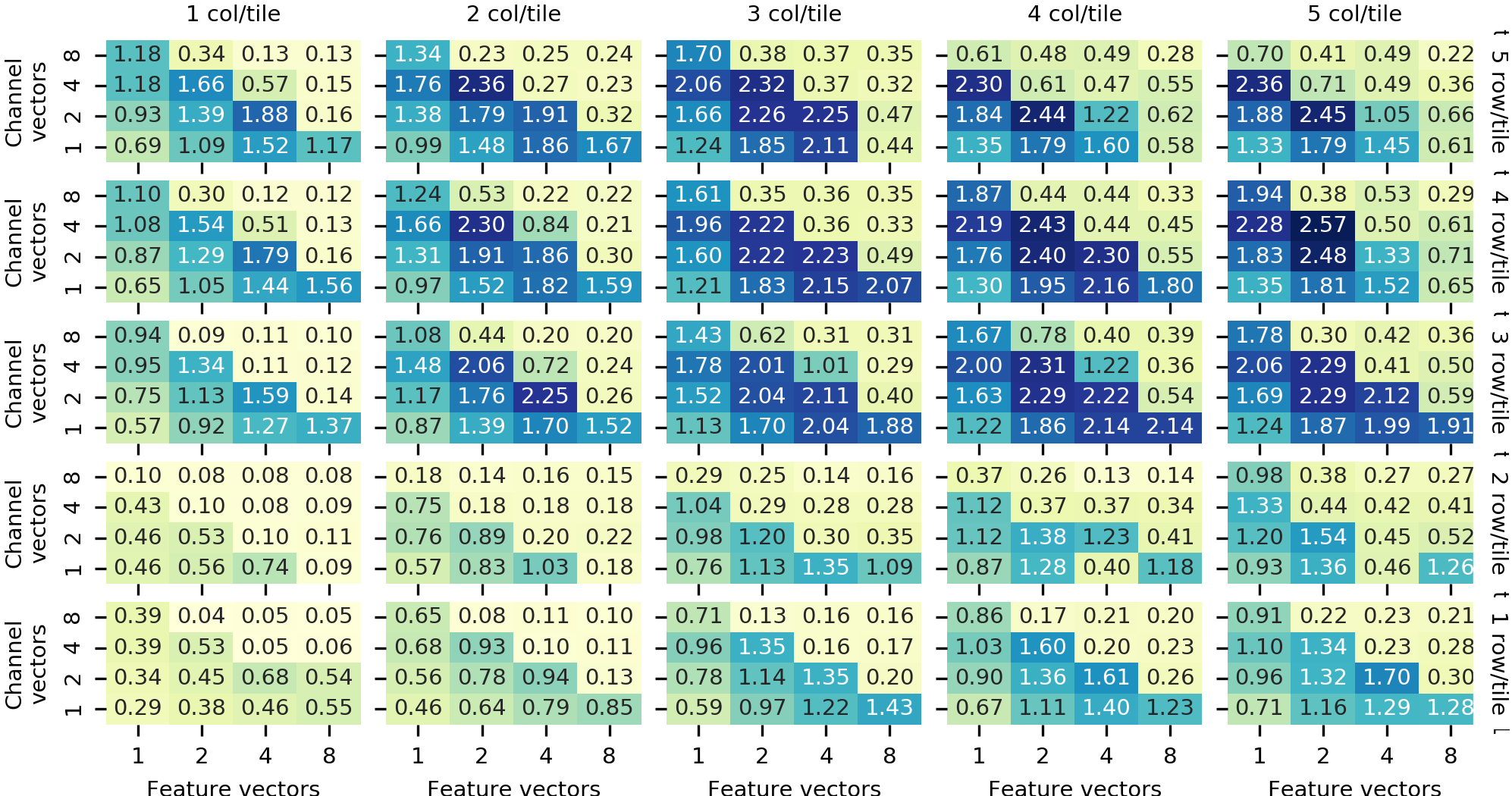
A comparison to Figure 2 where instead of register usage, the achieved performance is shown. The number of flops increases as tile sizes increase and as vector sizes increase, however in each heatmap there is a point where increasing vector sizes causes the performance to drop significantly. This often happens when using 8 element vectors.

Figure 3. Number of teraflops achieved for different tile sizes and vector sizes for a given 3$\times$3 convolution. Each subplot gives the performance for a given tile size as the vector sizes vary. Performance data obtained using an AMD R9 Nano GPU, with amdgpu-pro divers.

Adjacent elements in the convolution output require overlapping slices of the input tensor, so using a single thread to compute a number of these elements will reduce the number of times a single input element is loaded from memory. We refer to this as a tiled algorithm, as each thread will compute a tile of the output. As the tile size increases the number of times each input element is reused also increases and so the total number of bytes read from memory in the whole operation decreases. Memory bandwidth is typically the largest bottleneck in these GPU computations, as discussed in Section 2.2, and so reducing the number of loads typically improves performance accordingly. Similarly the use of vector loads and stores, as well as vector math operations, can improve performance on some devices.

The downside of using large tiles and vectors in GPU kernels is that each significantly increases the number of registers required to hold the data required for a single thread. As an example, Figure 2 shows the number of registers required for varying tile and vector sizes as provided by AMD’s CodeXL tools (cod, [n. d.]).

As GPUs have a limited number of registers available in their register files, the number of registers required by a single thread determines how many threads can be concurrently executed. Overhead and memory fetches are largely hidden in a GPU by quickly switching threads when one becomes stalled. If each thread requires more registers then the number of concurrent threads decreases and so the chance that one is ready to execute as soon as another is stalled is also decreased.

The best performance then does not necessarily come when using the largest tile sizes to get the most data reuse and large vector sizes to get more efficient loads and instruction level parallelism, but also the best performance is not achieved when using the fewest registers and so allowing the GPU to run the most threads concurrently.

Optimal performance is typically achieved by balancing these three factors, as shown in Figure 3 where the peak performance on the AMD R9 Nano is achieved using a $4\times 5$ tile, $4$ element vectors for input channels and $2$ element vectors for output channels (at $2.57$ teraflops), which gives a $10\times$ speed up over the naive implementation (at $0.29$ teraflops). When a tile size which uses more registers than are available on the device—and so any values in the registers are instead stored in memory—the performance is worse still, going down to as little as $50$ gigaflops.

On different devices, the optimal tile sizes and vector widths to get best performance will differ depending on the device’s load-store units, the number of available registers and whether vector math units are available.

Table 2. SYCL-BLAS configuration for local and register tile sizes. ‘Registers’ shows the number of registers in the tile, ‘Work group’ shows the work-group size used and ‘Local mem’ refers to the size of local memory used.

Configuration	Registers	Work group	Local mem
4$\times$4_8$\times$8_loc	16	64	8 KiB
4$\times$4_16$\times$16_loc	16	256	16 KiB
8$\times$4_8$\times$16_loc	32	128	16 kiB
8$\times$2_4$\times$16_loc	16	64	8 KiB
8$\times$4_8$\times$16_noloc	32	128	N/A
8$\times$4_4$\times$8_noloc	32	32	N/A
4$\times$4_8$\times$8_noloc	16	64	N/A

4.1.2. Winograd technique for fast convolutions

Lavin and Gray suggested a technique to accelerate convolutions in (Lavin and Gray, 2016) by using a transform studied by Winograd (Winograd, 1980) as well as Cook and Toom. In many DNN libraries this is referred to as the Winograd technique.

The technique involves transforming the input and filter tensors into a number of small matrices, then the convolution is computed using a batched matrix multiply between these matrices, followed by another transform to yield the output values. In this way the total number of floating point operations required to compute the convolution can be decreased to as little as $30\%$ of that required by a naive computation.

For a convolution with a $R\times S$ filter size, the input transform converts an $M\times N$ tile of the input tensor to a $(M+R-1)\times(N+S-1)$ tile, which is then scattered across $(M+R-1)(N+S-1)$ matrices with one tile element equal to an corresponding element in one of the matrices.

Increasing the tile sizes used in the transforms increases the amount of data reuse, so overall fewer memory fetches are required as discussed in Section 4.1.1. However larger tile sizes also require more registers as above, which can lead to fewer concurrent threads and possibly worse performance.

Another effect of using larger tiles sizes is that the number of intermediate matrices increases, but the size of each individual matrix decreases. The majority of the computation is the batched matrix multiply, and for smaller matrices it can be harder to fully utilize a GPU even with specialized batched kernels.

Given these considerations, there is again the problem of balancing the tile size with register usage, optimal matrix multiply sizes and vector widths in order to get the best performance. As with the tiled convolution computations, this will differ depending on the device as well as the optimizations available in the matrix multiplies. The performance portability provided by the SYCL-BLAS matrix multiplies discussed in Section 3 significantly affects the achievable performance when using this technique to compute convolutions.

5. Performance

The performance of our SYCL kernels is measured against hand-tuned, vendor provided libraries. The primary target devices of our libraries have been embedded devices, so the main comparison has been made to ARM’s ComputeLibrary (acl, [n. d.], v18.11). This provides accelerated routines through both NEON instructions for the CPU and OpenCL kernels for GPUs.

We also provide comparisons for Intel hardware, utilizing both the CPU and GPU, with comparisons to Intel MKL-DNN (mkl, [n. d.], v0.18.1) and to clBLAST (Nugteren, 2018).

5.1. Benchmark device setup

The performance benchmarks are provided on a range of hardware, to show the portability of our SYCL libraries.

5.1.1. HiSilicon Kirin 960

The HiSilicon HiKey 960 is a development board featuring the HiSilicon Kirin 960 system on a chip (SoC) designed for use in mobile phones. This comprises an ARM big.LITTLE CPU with 4 ARM A73 cores and 4 ARM A53 cores, along with an ARM Mali G-71 GPU.

When benchmarking using the GPU, the big (A73) CPUs are disabled to help keep device temperatures low. For benchmarking on the CPU, the big A73 cores are enabled.

5.1.2. Intel i7-6700K

The i7-6700K is a Skylake desktop processor which contains 4 CPU cores with a base frequency of 4GHz, boosting to 4.2GHz, and an Intel HD Graphics 530 integrated GPU with a base frequency of 350 MHz, boosting to 1.15GHz.

For the neural network benchmarks in Section 5.3, we benchmarked SYCL-DNN using both the CPU and GPU in the i7-6700K processor, as Intel provide an OpenCL implementation for Xeon and Core CPUs and an open source Graphics Compute Runtime for their integrated graphics processors. When benchmarking using the CPU the scaling governor was set to ‘performance’.

5.1.3. Intel i7-9700K

The i7-9700K is a Skylake desktop processor which contains 8 CPU cores with a base frequency of 3.6GHz, boosting to 4.9GHz, and an Intel UHD Graphics 630 integrated GPU with a base frequency of 350 MHz, boosting to 1.2GHz.

For the BLAS benchmarks in Section 5.2, we benchmarked only the GPU in the i7-9700K processor.

5.2. SYCL-BLAS GEMM benchmarks

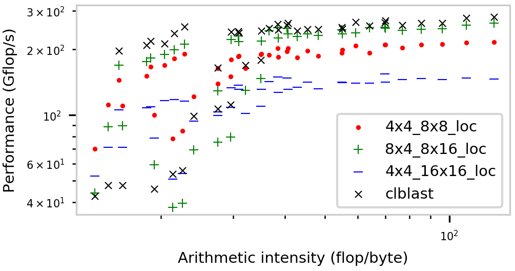
A scatter plot showing a roofline comparison of the arithmetic intensity in operations per byte with the total performance in operations per second. Each matrix multiply is computed with different configurations and compared to clBLAST. The clBLAST figures perform best, though only around 20 gigaflops ahead of one of the SYCL-BLAS configurations. The other configurations perform worse.

(a) Overall performance comparison of SYCL-BLAS for a number of tile configurations against hand-tuned clBLAST.

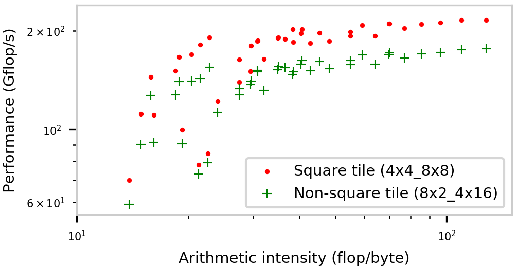
A roofline comparison between two SYCL-BLAS configurations one with a square 4 by 4 register tile and the other with an 8 by 2 tile. The square tile performs best in all cases.

(b) Performance comparison of using a square register tile vs a non-square register tile, when the total number of registers is constant.

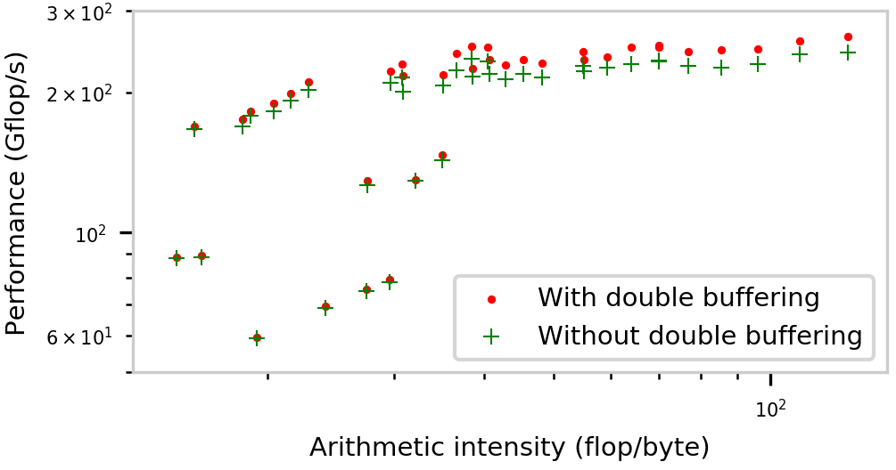
A roofline comparison between the same SYCL-BLAS configuration with and without double buffering. Using double buffering gives better performance in all cases shown.

(c) Performance comparison of using double buffering. Figures shown with configuration 8$\times$4_8$\times$16_loc.

Figure 4. Comparison of different performance metrics of SYCL-BLAS on an Intel UHD Graphics 630 GPU.

A comparison similar to the roofline model (Williams et al., 2009) is carried out to plot performance of a kernel (Gflop/s) as a function of its operational intensity, i.e the number of floating point operations per byte of data read or written (flop/byte).

The SYCL-BLAS GEMM implementation has been compared to clBLAST’s hand-tuned GEMM OpenCL kernels (Nugteren, 2018) on an Intel UHD Graphics 630 GPU and to ARM Compute Library’s GEMM kernels on an ARM Mali G-71 GPU. For each platform, different configurations of SYCL-BLAS have been used, with various register tile sizes, work-group sizes, and local memory sizes, as shown in Table 2. Each configuration contains h$\times$w_r$\times$c where h$\times$w represents a tile of $h$ by $w$ registers per thread to compute the block matrix $C_{ij}$, and r$\times$c represents a work-group consisting of $r\times c$ threads.

The number of data elements stored in local memory for the computation of a matrix multiply between matrices of size $M\times K$ and $K\times N$, for a configuration hxw_rxc is given by:

$$h\times r\times X+X\times w\times c$$

where $X$ is the number of data elements that fit within a cache line. The local memory size is doubled when double buffering is used. In Figures 4 and 5 each point represents the performance of a single matrix multiply between matrices of size $M\times K$ and $K\times N$, where $M\in[64,1204]$, $N\in[64,1024]$, $K\in[64,1024]$ and $M$, $N$, and $K$ are all powers of 2.

5.2.1. Performance on Intel i7-9700K

Figure 4(a) shows a roofline model comparing different configurations of SYCL-BLAS GEMM implementation against the GEMM implementation from clBLAST (Nugteren, 2018). Comparing these results shows that the 8$\times$4_8$\times$16_loc configuration for SYCL-BLAS achieves close to the performance of the hand-tuned clBLAST OpenCL kernels on the Intel GPU. In addition, the results show that increasing the number of registers from $4\times 4$ to $8\times 4$ per thread significantly improves performance, as data reuse is increased.

Figure 4(b) shows a roofline model comparing two different SYCL-BLAS GEMM configurations which use 16 registers, but in different tile layouts. The result shows that the square register tile 4$\times$4_8$\times$8 yields better performance than the non-square register tile 8$\times$2_4$\times$16, as discussed in Section 3.1.2. Similarly, Figure 4(c) shows the performance improvement from using double buffering to hide memory latency.

5.2.2. Performance on ARM HiKey 960

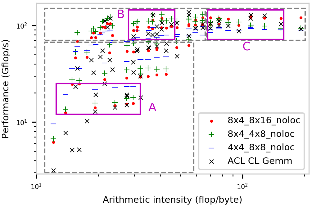
A large scatter plot showing a roofline comparison of 3 SYCL-BLAS configurations with ARM Compute Library. There are three highlighted zones, the one marked A is in the lower left corner, one marked B is in the upper center and one marked C is in the upper right corner.

(a) Overall comparison of SYCL-BLAS against the hand-tuned OpenCL kernels in ARM’s Compute Library across a variety of matrix sizes. The highlighted areas are shown in more detail below.

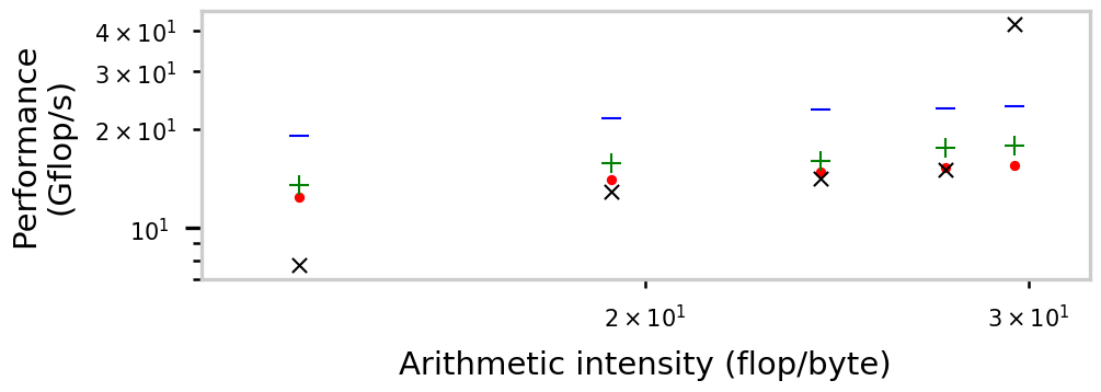
A more detailed view of zone A from Figure 5(a) showing that the SYCL-BLAS configuration with 4 by 4 register tiles performs the best, achieving around 20 gigaflops whereas ARM Compute Library achieves between 8 and 16.

(b) Block A, where 4$\times$4_8$\times$8 achieves the best performance.

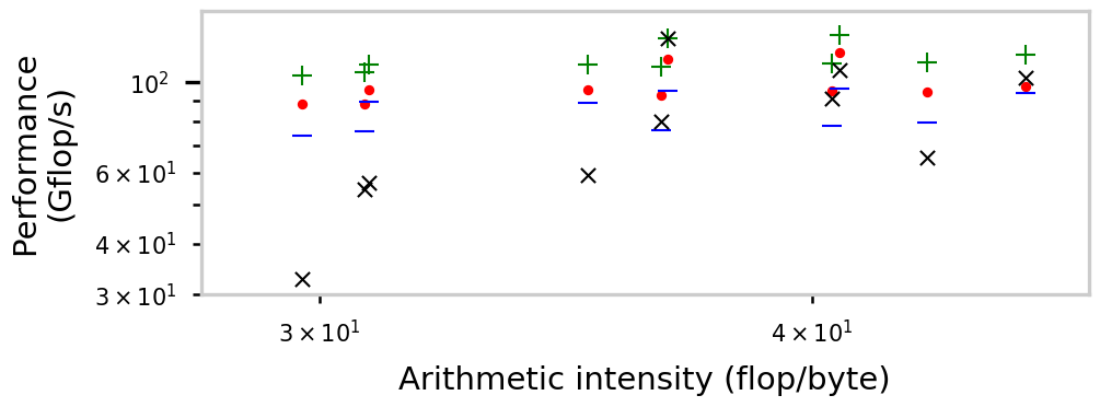
A more detailed view of zone B from Figure 5(a) showing that the SYCL-BLAS configuration with 8 by 4 register tiles performs the best, achieving between 100 and 140 gigaflops.

(c) Block B where 8$\times$4_4$\times$8 achieves the best performance.

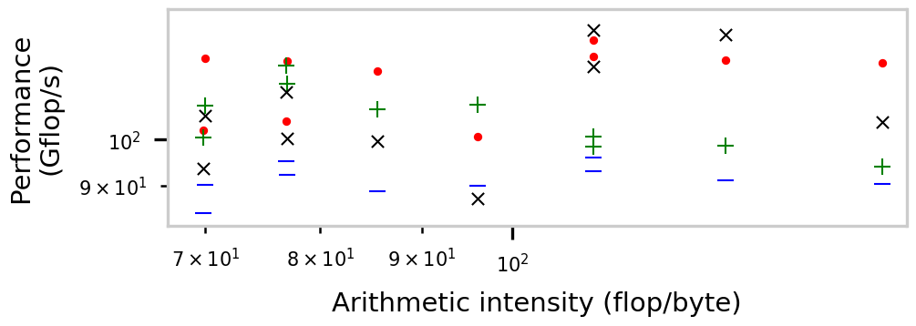
A more detailed view of zone C from Figure 5(a) showing that the SYCL-BLAS configuration with 8 by 4 register tiles but a larger work-group size performs the best in most cases, achieving between 100 and 140 gigaflops. In these cases with larger matrices, ARM Compute Library is more competitive and in some of the cases outperforms SYCL-BLAS.

(d) Block C where 8$\times$4_8$\times$16 achieves the best performance.

Figure 5. Roofline performance comparison of SYCL-BLAS on an ARM Mali G-71 GPU, compared to ARM’s Compute Library.

Figure 5(a) shows a roofline model comparing the number of gigaflops achieved by different configurations of SYCL-BLAS GEMM with that achieved by hand-tuned OpenCL kernels in ARM Compute Library. The figure is divided in 3 dotted regions where different GEMM configurations give better performance. These regions are shown in more detail in Figures 5(b) to 5(d).

In the region marked A, shown in Figure 5(b), the matrices have a small size and are typically square, so the matrix multiply has a low computational intensity and so comparatively few floating point operations. The 4$\times$4_8$\times$8 configuration shows the best performance for SYCl-BLAS, and is competitive with ARM Compute Library. However, in the region marked B, Figure 5(c), the 8$\times$4_4$\times$8 configuration is better. Here the matrices are small to medium sized and typically rectangular, so the operation has a higher computational intensity but still comparatively few operations, so launching fewer threads with a higher workload works well.

Figure 5(d) shows the region marked as C in more detail, where the matrices are large and so the operation has high computational intensity and many floating point operations. In this region the 8$\times$4_16$\times$8 configuration is best, as the larger matrices can be split up much better across a larger number of threads.

5.3. Neural network benchmarks

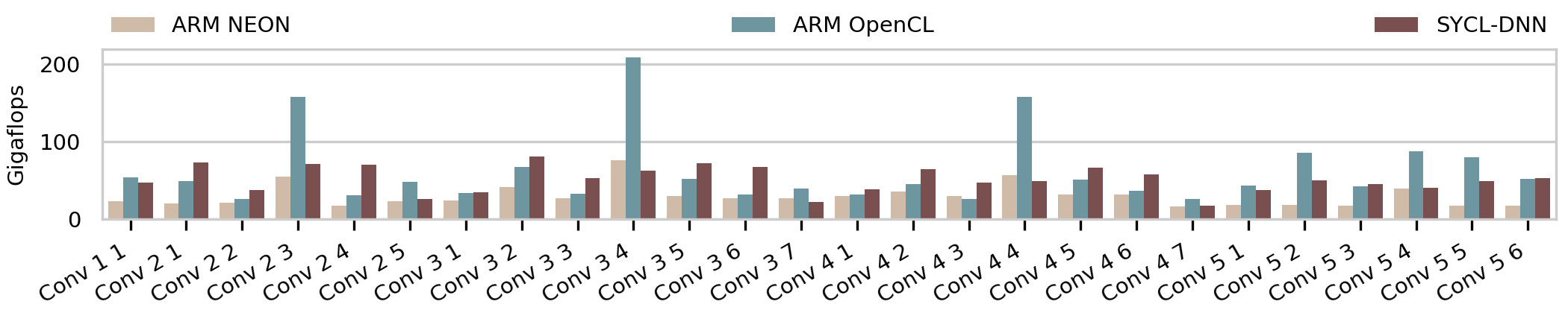
A bar chart with 26 groups of convolutions. In most cases SYCL-DNN performs better than ARM Compute Library by around 20 gigaflops, achieving between 40 and 80 gigaflops. The NEON implementation performs worst in almost all cases. There are three convolutions, corresponding to those with window size 3, where ARM Compute Library performs significantly better with between 150 and 200 gigaflops.

Figure 6. Gigaflop comparison for ResNet layers on ARM Hikey 960 with SYCL-DNN and ARM Compute Library on both CPU using NEON and GPU using OpenCL. Benchmark run with a batch size of 1.

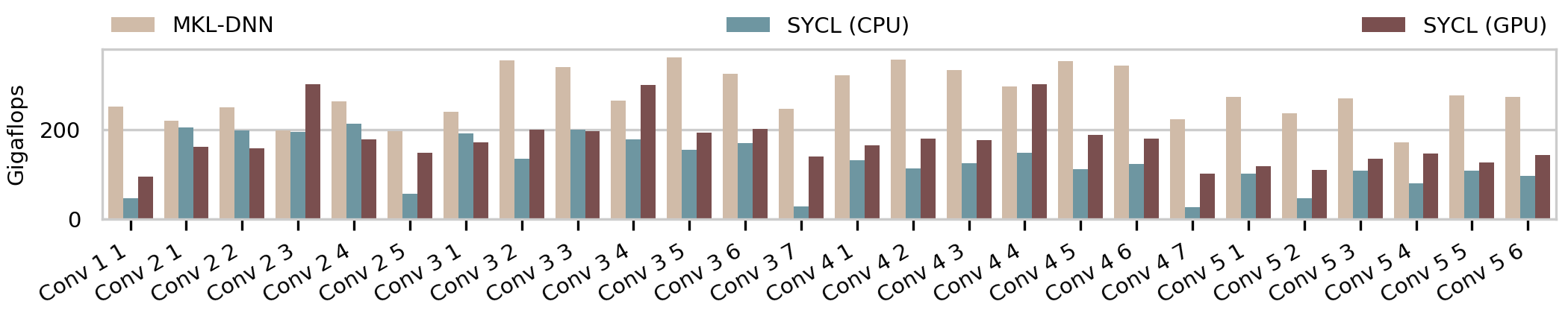
A bar chart with 26 groups of convolutions. In most cases MKL-DNN performs better than SYCL-DNN, achieving between 200 to 400 gigaflops, while SYCL-DNN can only achieve 150 to 300 gigaflops.

Figure 7. Gigaflop comparison for ResNet layers on Intel i7-6700K with SYCL-DNN on both CPU and GPU compared to MKL-DNN on the CPU. Benchmark run with a batch size of 4.

Table 3. Convolution sizes and parameters for each of the distinct layers in the VGG neural network model. The W column refers to the window size, S to the stride.

Layer	W	S	Input	Output
Conv 1 1	$3$	$1$	224 $\times$ 224 $\times$ 3	224 $\times$ 224 $\times$ 64
Conv 1 2	$3$	$1$	224 $\times$ 224 $\times$ 64	224 $\times$ 224 $\times$ 64
Conv 2 1	$3$	$1$	112 $\times$ 112 $\times$ 64	112 $\times$ 112 $\times$ 128
Conv 2 2	$3$	$1$	112 $\times$ 112 $\times$ 128	112 $\times$ 112 $\times$ 128
Conv 3 1	$3$	$1$	56 $\times$ 56 $\times$ 128	56 $\times$ 56 $\times$ 256
Conv 3 2	$3$	$1$	56 $\times$ 56 $\times$ 256	56 $\times$ 56 $\times$ 256
Conv 4 1	$3$	$1$	28 $\times$ 28 $\times$ 256	28 $\times$ 28 $\times$ 512
Conv 4 2	$3$	$1$	28 $\times$ 28 $\times$ 512	28 $\times$ 28 $\times$ 512
Conv 5 1	$3$	$1$	14 $\times$ 14 $\times$ 512	14 $\times$ 14 $\times$ 512

Table 4. Convolution sizes and parameters for each of the distinct layers in the ResNet neural network model. The W column refers to the window size, S to the stride.

Layer	W	S	Input	Output
Conv 1 1	$7$	$2$	230 $\times$ 230 $\times$ 3	112 $\times$ 112 $\times$ 64
Conv 2 1	$1$	$1$	56 $\times$ 56 $\times$ 64	56 $\times$ 56 $\times$ 256
Conv 2 2	$1$	$1$	56 $\times$ 56 $\times$ 64	56 $\times$ 56 $\times$ 64
Conv 2 3	$3$	$1$	56 $\times$ 56 $\times$ 64	56 $\times$ 56 $\times$ 64
Conv 2 4	$1$	$1$	56 $\times$ 56 $\times$ 256	56 $\times$ 56 $\times$ 64
Conv 2 5	$3$	$2$	56 $\times$ 56 $\times$ 64	28 $\times$ 28 $\times$ 64
Conv 3 1	$1$	$1$	28 $\times$ 28 $\times$ 64	28 $\times$ 28 $\times$ 256
Conv 3 2	$1$	$1$	28 $\times$ 28 $\times$ 256	28 $\times$ 28 $\times$ 512
Conv 3 3	$1$	$1$	28 $\times$ 28 $\times$ 256	28 $\times$ 28 $\times$ 128
Conv 3 4	$3$	$1$	28 $\times$ 28 $\times$ 128	28 $\times$ 28 $\times$ 128
Conv 3 5	$1$	$1$	28 $\times$ 28 $\times$ 128	28 $\times$ 28 $\times$ 512
Conv 3 6	$1$	$1$	28 $\times$ 28 $\times$ 512	28 $\times$ 28 $\times$ 128
Conv 3 7	$3$	$2$	28 $\times$ 28 $\times$ 128	14 $\times$ 14 $\times$ 128
Conv 4 1	$1$	$1$	14 $\times$ 14 $\times$ 128	14 $\times$ 14 $\times$ 512
Conv 4 2	$1$	$1$	14 $\times$ 14 $\times$ 512	14 $\times$ 14 $\times$ 1024
Conv 4 3	$1$	$1$	14 $\times$ 14 $\times$ 512	14 $\times$ 14 $\times$ 256
Conv 4 4	$3$	$1$	14 $\times$ 14 $\times$ 256	14 $\times$ 14 $\times$ 256
Conv 4 5	$1$	$1$	14 $\times$ 14 $\times$ 256	14 $\times$ 14 $\times$ 1024
Conv 4 6	$1$	$1$	14 $\times$ 14 $\times$ 1024	14 $\times$ 14 $\times$ 256
Conv 4 7	$3$	$2$	14 $\times$ 14 $\times$ 256	7 $\times$ 7 $\times$ 256
Conv 5 1	$1$	$1$	7 $\times$ 7 $\times$ 256	7 $\times$ 7 $\times$ 1024
Conv 5 2	$1$	$1$	7 $\times$ 7 $\times$ 1024	7 $\times$ 7 $\times$ 2048
Conv 5 3	$1$	$1$	7 $\times$ 7 $\times$ 1024	7 $\times$ 7 $\times$ 512
Conv 5 4	$3$	$1$	7 $\times$ 7 $\times$ 512	7 $\times$ 7 $\times$ 512
Conv 5 5	$1$	$1$	7 $\times$ 7 $\times$ 512	7 $\times$ 7 $\times$ 2048
Conv 5 6	$1$	$1$	7 $\times$ 7 $\times$ 2048	7 $\times$ 7 $\times$ 512

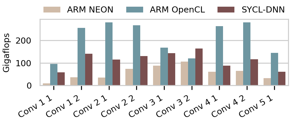
A bar chart showing the 9 convolutions in VGG. In all but one case ARM Compute Library performs best. SYCL-DNN achieves between 90 and 150 gigaflops, which ARM Compute Library varies more achieving between 100 and 280. The NEON implementation performs the worst reaching a maximum of around 100 gigaflops.

Figure 8. Gigaflop comparison for VGG layers on ARM Hikey 960 with SYCL-DNN and ARM Compute Library on both CPU using NEON and GPU using OpenCL. Benchmark run with a batch size of 1.

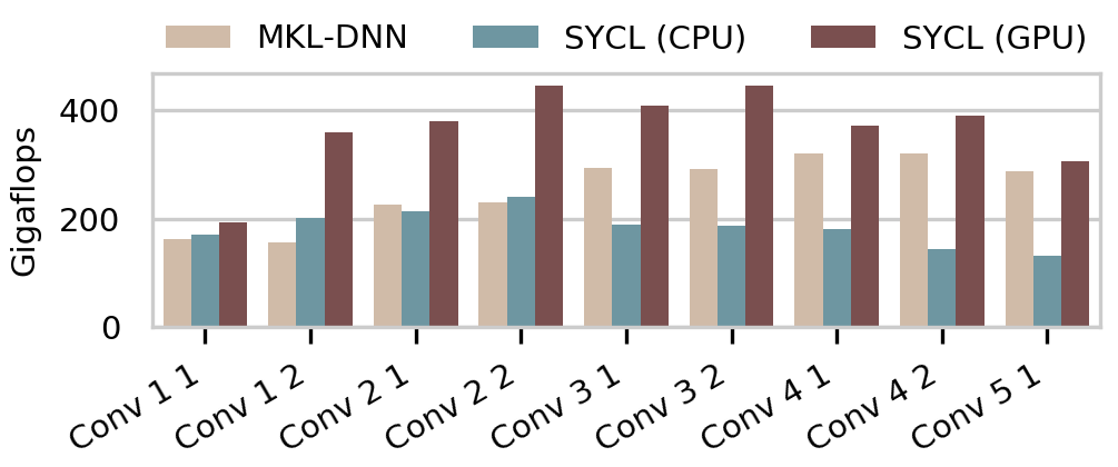
A bar chart showing the 9 convolutions in VGG. SYCL-DNN performs the best using the GPU, achieving 200 gigaflops in the first convolution and between 300 and 420 in the others. MKL-DNN achieves between 180 and 300 gigaflops.

Figure 9. Gigaflop comparison for VGG layers on Intel i7-6700K with SYCL-DNN on CPU and GPU compared to MKL-DNN on the CPU. Benchmark run with a batch size of 4.

To determine the performance of SYCL-DNN compared to other neural network acceleration libraries we extracted the convolution layers from well known standard image recognition networks. The networks chosen are VGG-16 (Simonyan and Zisserman, 2014) and ResNet-50 (He et al., 2016), introduced in 2014 and 2015 respectively, which are fairly large convolutional networks which were state-of-the-art when introduced, and are still frequently used as they provide good results and are widely available.

The VGG model uses 16 layers of 3$\times$3 convolutions interspersed with max pooling layers, while the ResNet model is made up of a number of blocks each consisting of a 1$\times$1 convolution, a 3$\times$3 convolution then a 1$\times$1 convolution. Exact sizes for these layers as used in the benchmarks are shown in Table 3 and 4.

The performance results for the HiKey 960 SoC are shown in Figures 8 and 6 for the VGG and ResNet benchmarks respectively. SYCL-DNN is competitive with ARM’s compute library and typically out performs both the OpenCL and Neon implementations in the ResNet benchmarks. The VGG model makes use of more 3$\times$3 convolutions, which have very optimized OpenCL implementations in the ARM library and in most cases outperform SYCL-DNN. These 3$\times$3 convolutions are also the three cases that stand out in the ResNet benchmark where the ARM OpenCL performance is significantly higher.

Figures 9 and 7 show the performance of the VGG and ResNet benchmarks on the Intel i7-6700K platform, comparing the performance of SYCL-DNN on both the CPU and the GPU against MKL-DNN. For the convolutions in the ResNet model MKL-DNN is consistently faster than SYCL-DNN, achieving up to 366 gigaflops while SYCL-DNN achieves a maximum of 244. However in the VGG benchmark SYCL-DNN running on the GPU consistently outperforms MKL-DNN.

6. Conclusion

The SYCL programming model allows us to write highly parametrized compute kernels, which can be instantiated to best suit the targeted hardware and so obtain good performance across different hardware.

Overall, we have shown that our general purpose, parameterized SYCL kernels give competitive performance against hand tuned, optimized libraries such as clBLAST, ARM Compute Library and MKL-DNN. Moreover these kernels can be easily tuned to perform well on other devices, even if they have significantly different performance characteristics.

There are many improvements still to make to these libraries, including adding vector operations to SYCL-BLAS and implementations of convolution kernels in SYCL-DNN which support data prefetching and local memory, as well as providing currently unsupported operations required for neural networks. There are also plans to develop a machine learning system to tune these libraries for new devices.

References

- (1)
- cod ([n. d.]) [n. d.]. AMD CodeXL GPU profiler and tool suite. https://gpuopen.com/compute-product/codexl/. Accessed: 2019-04-01.
- acl ([n. d.]) [n. d.]. The ARM Computer Vision and Machine Learning library. https://github.com/ARM-software/ComputeLibrary/. Accessed: 2019-03-19.
- com ([n. d.]) [n. d.]. ComputeCpp. https://www.codeplay.com/products/computesuite/computecpp. Accessed: 2019-03-19.
- gre ([n. d.]) [n. d.]. Green500 list of most energy efficient supercomputers in the world. https://www.top500.org/green500/lists/2018/11/. Accessed: 2019-03-19.
- mio ([n. d.]) [n. d.]. MIOpen: AMD’s Machine Intelligence Library. https://github.com/ROCmSoftwarePlatform/MIOpen. Accessed: 2019-04-01.
- mkl ([n. d.]) [n. d.]. MKL-DNN: Intel Math Kernel Library for Deep Neural Networks. https://github.com/intel/mkl-dnn. Accessed: 2019-04-09.
- bla ([n. d.]) [n. d.]. Netlib BLAS: Basic Linear Algebra Subprograms. http://www.netlib.org/blas/. Accessed: 2019-03-19.
- nvi ([n. d.]a) [n. d.]a. NVIDIA cuBLAS: Dense Linear Algebra on GPUs. https://developer.nvidia.com/cublas. Accessed: 2019-04-09.
- nvi ([n. d.]b) [n. d.]b. NVIDIA CUDA C Programming Guide v10.1.105. https://docs.nvidia.com/cuda/cuda-c-programming-guide/index.html. Accessed: 2019-04-01.
- cud ([n. d.]) [n. d.]. NVIDIA CUDA programming model. http://www.nvidia.com/CUDA. Accessed: 2019-03-19.
- syc ([n. d.]a) [n. d.]a. SYCL-BLAS: An implementation of BLAS using the SYCL open standard. https://github.com/CodeplaySoftware/SYCL-BLAS. Accessed: 2019-04-09.
- syc ([n. d.]b) [n. d.]b. SYCL: C++ Single-source Heterogeneous Programming for OpenCL. https://www.khronos.org/sycl/. Accessed: 2019-03-11.
- syc ([n. d.]c) [n. d.]c. The SYCL-DNN neural network acceleration library. https://github.com/CodeplaySoftware/SYCL-DNN. Accessed: 2019-04-09.
- syc ([n. d.]d) [n. d.]d. SYCL-PRNG: A pseudo random number generator library written against the SYCL API. https://github.com/Wigner-GPU-Lab/SYCL-PRNG. Accessed: 2019-04-01.
- top ([n. d.]) [n. d.]. TOP500 list of fastest supercomputers in the world. https://www.top500.org/lists/2018/11/. Accessed: 2019-03-19.
- vis ([n. d.]) [n. d.]. VisionCpp: A machine vision library written in SYCL and C++. https://github.com/codeplaysoftware/VisionCpp. Accessed: 2019-04-01.
- Abadi et al. (2015) Martín Abadi, Ashish Agarwal, Paul Barham, Eugene Brevdo, Zhifeng Chen, Craig Citro, Greg S. Corrado, Andy Davis, Jeffrey Dean, Matthieu Devin, Sanjay Ghemawat, Ian Goodfellow, Andrew Harp, Geoffrey Irving, Michael Isard, Yangqing Jia, Rafal Jozefowicz, Lukasz Kaiser, Manjunath Kudlur, Josh Levenberg, Dandelion Mané, Rajat Monga, Sherry Moore, Derek Murray, Chris Olah, Mike Schuster, Jonathon Shlens, Benoit Steiner, Ilya Sutskever, Kunal Talwar, Paul Tucker, Vincent Vanhoucke, Vijay Vasudevan, Fernanda Viégas, Oriol Vinyals, Pete Warden, Martin Wattenberg, Martin Wicke, Yuan Yu, and Xiaoqiang Zheng. 2015. TensorFlow: Large-Scale Machine Learning on Heterogeneous Systems. https://www.tensorflow.org/ Software available from tensorflow.org.
- Aliaga et al. (2017) José I. Aliaga, Ruymán Reyes, and Mehdi Goli. 2017. SYCL-BLAS: Leveraging Expression Trees for Linear Algebra. In Proceedings of the 5th International Workshop on OpenCL (IWOCL 2017). ACM, New York, NY, USA, Article 32, 5 pages. https://doi.org/10.1145/3078155.3078189
- Chetlur et al. (2014) Sharan Chetlur, Cliff Woolley, Philippe Vandermersch, Jonathan Cohen, John Tran, Bryan Catanzaro, and Evan Shelhamer. 2014. cuDNN: Efficient Primitives for Deep Learning. CoRR abs/1410.0759 (2014). arXiv:1410.0759
- Goli (2016) Mehdi Goli. 2016. VisionCPP: A SYCL-based Computer Vision Framework. In Proceedings of the 4th International Workshop on OpenCL (IWOCL ’16). ACM, New York, NY, USA, Article 6, 4 pages. https://doi.org/10.1145/2909437.2909444
- Goli (2017) Mehdi Goli. 2017. SYCL backend for Eigen. In Technical peresentation in 1st workshop on Distributed and Heterogeneous Programming in C and C++ (DHPCC++ 17)—to appear in May.
- Goli et al. (2018) Mehdi Goli, Luke Iwanski, John Lawson, Uwe Dolinsky, and Andrew Richards. 2018. TensorFlow Acceleration on ARM Hikey Board. In Proceedings of the International Workshop on OpenCL (IWOCL ’18). ACM, New York, NY, USA, Article 7, 4 pages. https://doi.org/10.1145/3204919.3204926
- Goli et al. (2017) Mehdi Goli, Luke Iwanski, and Andrew Richards. 2017. Accelerated Machine Learning Using TensorFlow and SYCL on OpenCL Devices. In Proceedings of the 5th International Workshop on OpenCL (IWOCL 2017). ACM, New York, NY, USA, Article 8, 4 pages. https://doi.org/10.1145/3078155.3078160
- Guennebaud et al. (2010) Gaël Guennebaud, Benoît Jacob, et al. 2010. Eigen v3. http://eigen.tuxfamily.org.
- Gustavson et al. (1998) Fred G. Gustavson, André Henriksson, Isak Jonsson, Bo Kågström, and Per Ling. 1998. Recursive Blocked Data Formats and BLAS’s for Dense Linear Algebra Algorithms. In Proceedings of the 4th International Workshop on Applied Parallel Computing, Large Scale Scientific and Industrial Problems (PARA ’98). Springer-Verlag, London, UK, UK, 195–206. http://dl.acm.org/citation.cfm?id=645781.666659
- He et al. (2016) K. He, X. Zhang, S. Ren, and J. Sun. 2016. Deep Residual Learning for Image Recognition. In 2016 IEEE Conference on Computer Vision and Pattern Recognition (CVPR). 770–778. https://doi.org/10.1109/CVPR.2016.90
- Kerr et al. ([n. d.]) Andrew Kerr, Duane Merrill, Julien Demouth, and John Tran. [n. d.]. CUTLASS: Fast linear algebra in CUDA C++. Nvidia Developer Blog, Dec 2017. https://devblogs.nvidia.com/cutlass-linear-algebra-cuda/.
- Lavin and Gray (2016) A. Lavin and S. Gray. 2016. Fast Algorithms for Convolutional Neural Networks. In 2016 IEEE Conference on Computer Vision and Pattern Recognition (CVPR). 4013–4021. https://doi.org/10.1109/CVPR.2016.435
- Nath et al. (2010) Rajib Nath, Stanimire Tomov, and Jack Dongarra. 2010. An Improved Magma Gemm For Fermi Graphics Processing Units. The International Journal of High Performance Computing Applications 24, 4 (2010), 511–515. https://doi.org/10.1177/1094342010385729
- Nugteren (2018) Cedric Nugteren. 2018. CLBlast: A Tuned OpenCL BLAS Library. In Proceedings of the International Workshop on OpenCL (IWOCL ’18). ACM, New York, NY, USA, Article 5, 10 pages. https://doi.org/10.1145/3204919.3204924
- Pheatt (2008) Chuck Pheatt. 2008. Intel® threading building blocks. Journal of Computing Sciences in Colleges 23, 4 (2008), 298–298.
- Reyes and Lomüller (2015) Ruyman Reyes and Victor Lomüller. 2015. SYCL: Single-source C++ accelerator programming. In PARCO. 673–682. https://doi.org/10.3233/978-1-61499-621-7-673
- Simonyan and Zisserman (2014) K. Simonyan and A. Zisserman. 2014. Very Deep Convolutional Networks for Large-Scale Image Recognition. CoRR abs/1409.1556 (2014). arXiv:1409.1556
- Stone et al. (2010) J. E. Stone, D. Gohara, and G. Shi. 2010. OpenCL: A Parallel Programming Standard for Heterogeneous Computing Systems. Computing in Science Engineering 12, 3 (May 2010), 66–73. https://doi.org/10.1109/MCSE.2010.69
- Wang et al. (2014) Endong Wang, Qing Zhang, Bo Shen, Guangyong Zhang, Xiaowei Lu, Qing Wu, and Yajuan Wang. 2014. Intel math kernel library. In High-Performance Computing on the Intel® Xeon Phi. Springer, 167–188.
- Williams et al. (2009) Samuel Williams, Andrew Waterman, and David Patterson. 2009. Roofline: An insightful visual performance model for floating-point programs and multicore architectures. Technical Report. Lawrence Berkeley National Lab.(LBNL), Berkeley, CA (United States).
- Winograd (1980) Shmuel Winograd. 1980. Arithmetic complexity of computations. Society for Industrial and Applied Mathematics. 93 pages. https://doi.org/10.1137/1.9781611970364.fm