Theory and implementation of event-triggered stabilization
over digital channels

Abstract

In the context of event-triggered control, the timing of the triggering events carries information about the state of the system that can be used for stabilization. At each triggering event, not only can information be transmitted by the message content (data payload) but also by its timing. We demonstrate this in the context of stabilization of a laboratory-scale inverted pendulum around its equilibrium point over a digital communication channel with bounded unknown delay. Our event-triggering control strategy encodes timing information by transmitting in a state-dependent fashion and can achieve stabilization using a data payload transmission rate smaller than what the data-rate theorem prescribes for classical periodic control policies that do not exploit timing information. Through experimental results, we show that as the delay in the communication channel increases, a higher data payload transmission rate is required to fulfill the proposed event-triggering policy requirements. This confirms the theoretical intuition that a larger delay brings a larger uncertainty about the value of the state at the controller, as less timing information is carried in the communication. Our results also provide a novel encoding-decoding scheme to achieve input-to-state practically stability (ISpS) for nonlinear continuous-time systems under appropriate assumptions.

I Introduction

Event-triggered control has gained significant attention due to its advantages over conventional control schemes in cyber-physical systems (CPS). Although periodic control is the most common and perhaps simplest solution for digital systems, it can be inefficient in sharing communication and computation resources [1, 2, 3, 4, 5, 6, 7, 8, 9, 10]. The central concept of event-triggered control is to transmit sensory data only when needed to satisfy the control objective. In addition to utilizing the distributed resources efficiently, it has been proven that carefully crafted event-triggered policies outperform the linear-quadratic (LQ) performance of the periodic control policies [11]. Another advantage of event-triggered control is that the timing of the triggering events, effectively revealing the state of the system, carries information that can be used for stabilization. This allows achieving stabilization with a transmission rate lower than that required by periodic control strategies [12, 13, 14].

In networked control systems a finite-rate digital communication channel closes the loop between the sensor and the controller. In this setting, data-rate theorems [15, 16, 17, 18, 19, 20, 21] provide the communication channel requirements for stabilization.

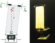
Figure 1: An inverted pendulum controlled by thrust force of two propellers. The pendulum is a plywood sheet of length $l$. The angle $\phi$ of the pendulum from the vertical line and its rate of change, measured by the sensor and transmitted to the controller over a digital channel with bounded unknown delay, are used to determine the left and right thrust forces $f_{L}$ and $f_{R}$ of the propellers.

They state that to ensure stabilization of an unstable linear system, the minimum information rate communicated over the channel, including both data payload and timing information, must be at least equal to the entropy rate of the plant, defined as the sum of the unstable modes in nats [12, 13]. When information is encoded in the timing of the transmission events using event-triggered control, our previous work [22, 23] has shown the existence of an event-triggering strategy that achieves input-to-state practically stability (ISpS) [24, 25] for any linear, time-invariant system subject to bounded disturbance over a digital communication channel with bounded delay using a data payload transmission rate lower than the entropy rate. This is possible because, for small values of the delay, the timing information is substantial, and the data payload transmission rate can be lower than the entropy rate of the plant. However, as the delay increases, a higher data payload transmission rate is required to satisfy the requirements of the proposed event-triggering control strategy.

A similar data-rate theorem formulation also holds for nonlinear systems. The works [26, 27, 28] for nonlinear systems are restricted to plants without disturbances and with a bit-pipe communication channel. The work [26] uses the entropy of topological dynamical systems to elegantly determine necessary and sufficient bit rates for local uniform asymptotic stability. Consequently, the results are only local and derived under restrictive assumptions. Under appropriate assumptions, the work [27] extends to nonlinear but locally Lipschitz systems, the zoom-in/zoom-out strategy of [29]. The sufficient condition proposed in this work is, however, conservative, and does not match the necessary condition proposed in [26]. The work [25] further extend the results in [27] to linear systems with uncertainty and under appropriate assumptions to nonlinear systems with disturbances. Inspired by the Jordan block decomposition employed in [16] to design an encoder/decoder pair of a vector system, the work [28] provides a sufficient design for feed-forward dynamics that matches the necessary condition proposed in [26]. The recent work in [30] studies the estimation of a nonlinear system over noisy communication channels, providing a necessary condition over memoryless communication channels and a sufficient condition in case of additive white Gaussian noise channel.

The majority of results on control under communication constraints are restricted to theoretical works. Here for the first time, we examine data-rate theorems in a practical setting, using an inverted pendulum, a classic example of an inherently unstable nonlinear plant with numerous practical applications. Our first contribution is to implement the event-triggering control design introduced in [22, 23], and demonstrate the utilization of timing information to stabilize a laboratory-scale inverted pendulum over a digital communication channel with bounded unknown delay, see Fig. 1. A video that illustrates the main ideas and demonstrates our experimental results can be found at https://youtu.be/1P0i-tWsPoA. The results of our experiments show that using the sufficient packet size derived in [22, 23] on a linearized model of the inverted pendulum around its unstable equilibrium point, the state estimation error is sufficiently small and we can stabilize the system. We show that for small values of the delay the experimental data payload transmission rate is lower than the entropy rate of the plant. On the other hand, by increasing the upper bound on the delay in the communication channel, higher data payload transmission rates are required to satisfy the requirements of the proposed control strategy. The event-triggering policy developed in [22, 23] can only stabilize the pendulum locally around its equilibrium point, where linearization is possible. Our second contribution is to address nonlinear systems directly, and develop a novel event-triggering scheme that exploits timing information to render a class of continuous-time nonlinear systems subject to disturbances ISpS.

From the system’s perspective, our set-up is closest to the one in [27, 25], as we consider locally Lipschitz nonlinear systems that can be made input-to-state stable (ISS) [31] with respect to the state estimation error and system disturbances. Using our encoding-decoding scheme, we encode the information in timing via event-triggering control in a state-dependent fashion to achieve input-to-state practical stability (ISpS) in the presence of unknown but bounded delay. We also discuss the different approaches to eliminate the ISS assumption.

Finally, we point out that the work [32] studies event-triggering stabilization of globally Lipschitz nonlinear system without disturbances where the communication delay is arbitrarily small. Also, the work [33] investigates event-triggered stabilization of nonlinear system under communication constraints but it does not explicitly quantify the effect of quantization in the presence of system disturbances, nor the timing information carried by the triggering events. In addition, the recent work [34] utilizes a time-triggered controller to stabilize a two-wheeled inverted pendulum around its upright position over IEEE 802.11g (WiFi). Since the whole bandwidth of this channel is devoted to a two-wheeled inverted pendulum, the work [34] does not explicitly examine the effect quantization.

A complete list of notations and proofs of all the results appear in the Appendix.

II System model

We consider the stabilization of the inverted pendulum depicted in Fig. 1 around its unstable equilibrium point. The sensory information for stabilization is sent to the controller over a digital channel. The block diagram of the control system is given in Fig. 2.

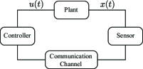
Figure 2: System model.

We assume the communication channel is capable of transmitting packets composed of a finite number of bits without error. Each transmitted packet is subject an unknown delay upper bounded by $\gamma\geq 0$. In addition to the data payload, the transmission time of the packets sent over the channel could be utilized to convey information to the controller. As a result, the encoding process consists of choosing the timing and data payload of the packet, as shown in Fig. 3. In other words, in the sensor block, the quantized version of the state is encoded in a packet containing data payload as well as its timing.

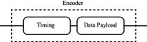
Figure 3: Representation of information transmission using data payload and transmission time of the packet in a digital channel. The encoding process consists of choosing the data payloads and their transmission times. Here, the sensor determines the transmission time using our event-triggering strategy in a state-dependent manner.

In our design, the sensor encodes information in timing via an event-triggering technique in a state-dependent fashion.

At each triggering event, occurring at times $\{t_{s}^{k}\}_{k\in\mathbb{N}}$, the sensor transmits a packet $p(t_{s}^{k})$ of length $g(t_{s}^{k})$ over the communication channel. Packets arrive at the controller at times $\{t_{c}^{k}\}_{k\in\mathbb{N}}$. When referring to a generic triggering or reception time, we skip the super-script $k$ in $t_{s}^{k}$ and $t_{c}^{k}$.

Since the delay in the communication channel is upper bounded by $\gamma\geq 0$, the communication delays represented by $\Delta_{k}=t_{c}^{k}-t_{s}^{k}$ ($k\in\mathbb{N}$) must satisfy

$$\Delta_{k}\leq\gamma.$$ (1)

By defining the $k^{th}$ triggering interval as $\Delta^{\prime}_{k}=t_{s}^{k+1}-t_{s}^{k}$, the information transmission rate (the rate at which sensor transmits data payload over the channel) can be defined as

$$R_{s}=\limsup_{N\rightarrow\infty}\frac{\sum_{k=1}^{N}g(t_{s}^{k})}{\sum_{k=1}^{N}\Delta^{\prime}_{k}}.$$ (2)

II-A Plant Dynamics

We consider a linearized version of the two-dimensional problem of balancing an inverted pendulum with two propellers, where the motion of the pendulum is constrained in a plane and its position can be measured by an angle $\phi$ representing small deviations from the upright position of the pendulum, as depicted in Fig. 1. The inverted pendulum has mass $m_{1}$ and length $l$. The propellers are identical and are attached to two motors of mass $m_{2}$. $m$ and $I$ respectively represent the total mass of the system and its moment of inertia. Therefore, a nonlinear equation of the system can be written as follows

$$I\ddot{\phi}=mgl\sin\phi(t)+\xi(t)l+\textrm{noise},$$ (3)

where $g$ is the gravitational acceleration, and $\xi(t)$ is the resultant thrust force of the propellers ($f_{L}$ and $f_{R}$ as shown in Fig. 1) generating a moment about the axis of rotation of the pendulum. Note that in this nonlinear equation the effect of the friction is included in the additive noise. The force $\xi(t)$ can be estimated as a linear function of the control input $\tilde{u}(t)$, applied to the motors, with some proportionality constant $k_{\xi}$ (found from experiments), namely $\xi(t)=k_{\xi}\tilde{u}(t)$.

We derive the linearized equations of motion using a small angle approximation. This linearization is only valid for sufficiently small values of the delay upper bound $\gamma$ in the communication channel. Linearizing (3) around the equilibrium point results in the following dynamics

$$I\ddot{\phi}=mgl\phi(t)+k_{\xi}l\tilde{u}(t)+\textrm{noise}.$$ (4)

By defining the state variable $\tilde{\boldsymbol{x}}=(\phi,\dot{\phi})^{T}$, the state-space equations can be written as follows

$$\dot{\tilde{\boldsymbol{x}}}=\tilde{\textbf{A}}\tilde{\boldsymbol{x}}+\tilde{\textbf{B}}\tilde{u}(t)+\tilde{\boldsymbol{w}}(t),$$ (5)

where

$$\textstyle\tilde{\textbf{A}}=\begin{bmatrix}0&1\\ \frac{mgl}{I}&0\end{bmatrix},\tilde{\textbf{B}}=\begin{bmatrix}0\\ \frac{k_{\xi}l}{I}\end{bmatrix}.$$ (6)

In our prototype shown in Fig. 1, the pendulum is a plywood sheet of size $0.18\times 0.073\times 0.005$ m and mass $m_{1}=0.030$ kg. The motors are of mass $m_{2}=0.010$ kg. Also, $l=0.180$ m, and $g=9.81$ m/s². Using first principles, one can find the moment of inertia of the pendulum about its axis of rotation to be $I=3.57\times 10^{-4}$ kg/m². By experiments, we approximate $k_{\xi}=0.001$. Therefore, the system (5) can be rewritten as follows

$$\textstyle\dot{\tilde{\boldsymbol{x}}}=\begin{bmatrix}0&1\\ 53.58&0\end{bmatrix}\tilde{\boldsymbol{x}}+\begin{bmatrix}0\\ 0.50\end{bmatrix}\tilde{u}(t)+\tilde{\boldsymbol{w}}(t).$$ (7)

Using (5) it follows $\tilde{w}_{1}(t)=0$. Also, by experiments we deduce $|w_{2}(t)|$ is upper bounded by $0.02$.

Now using the eigenvector matrix

$$\textstyle\textbf{P}=\begin{bmatrix}0.1354&-0.1354\\ 0.9908&0.9908\end{bmatrix}$$ (8)

of matrix $\tilde{\textbf{A}}$ we consider a canonical transformation to diagonalize the system (7) as follows

$$\dot{\boldsymbol{x}}=\textbf{A}\boldsymbol{x}(t)+\textbf{B}u(t)+\boldsymbol{w}(t),$$ (9)

where $\textbf{A}=\textbf{P}^{-1}\tilde{\textbf{A}}\textbf{P}$, $\textbf{B}=\textbf{P}^{-1}\tilde{\textbf{B}}$, $\boldsymbol{x}(t)=\textbf{P}^{-1}\tilde{\boldsymbol{x}}(t)$ and $\boldsymbol{w}(t)=\textbf{P}^{-1}\tilde{\boldsymbol{w}}(t)$. Therefore, for the diagonalized system (9) we have

$$\textstyle\textbf{A}=\begin{bmatrix}\lambda_{1}&0\\ 0&\lambda_{2}\end{bmatrix}=\begin{bmatrix}7.3198&0\\ 0&-7.3198\end{bmatrix},$$ (10)

$$\textstyle\textbf{B}=\begin{bmatrix}0.2523\\ 0.2523\end{bmatrix},\,\,\boldsymbol{x}=\begin{bmatrix}3.6940\phi+0.5046\dot{\phi}\\ 0.5046\dot{\phi}-3.6940\phi\end{bmatrix},$$ (11)

$$\textstyle|w_{i}(t)|\leq M=0.0470\,\,\>\textrm{for}\>i\in\{1,2\},$$ (12)

where the upper bound $M$ on the $|w_{i}(t)|$ for $i\in\{1,2\}$ is found by taking the maximum of upper bounds of all the elements in $\boldsymbol{w}(t)$.

We now define a modified version of input-to-state practically stablity (ISpS) [24, 25], which is suitable for our event-triggering setup with the unknown but bounded delay in the digital communication channel.

Definition 1

The plant (9) is ISpS if both of its coordinates $x_{1}(0)$ and $x_{2}(0)$ are ISpS. Also, $x_{1}(t)$ is ISpS if there exist $\beta\in\mathcal{KL}$, $\psi\in\mathcal{K}_{\infty}(0)$, $d\in{}_{\geq 0}$, $\chi\in\mathcal{K}_{\infty}(d)$, $d^{\prime}\in{}_{\geq 0}$ and $\zeta\in\mathcal{K}_{\infty}^{2}(0,d^{\prime})$ such that for all $t\geq 0$

$$|x_{1}(t)|\!\leq\!\beta\left(|x_{1}(0)|,t\right)\!+\!\psi\left(|w_{1}|_{t}\right)\!+\!\chi(\gamma)\!+\!\zeta(|w_{1}|_{t},\gamma).$$ (13)

Note that, for a fixed $\gamma$, this definition reduces to the standard notion of ISpS. Given that the initial condition, delay, and system disturbances are bounded, ISpS implies that the state must be bounded at all times beyond a fixed horizon.

Since $\lambda_{2}$ in (9) is negative, the second coordinate is inherently stable, and we do not need to transmit updates about the second coordinate to the controller via the communication channel. However, since $\lambda_{1}$ is positive, the uncertainty about the first coordinate grows exponentially at the controller, hence the sensor needs to communicate information to the controller about the state of the first coordinate to render the plant ISpS [22].

A brief description of the event-triggered control approach in our previous work [22, 23] which determines the sequence of transmission times $\{t_{s}^{k}\}_{k\in\mathbb{N}}$ and packets $\{p(t^{k}_{s})\}_{k\in\mathbb{N}}$ to achieve ISpS for the first coordinate of the dynamics (9) is available at Appendix -B.

III Implementation and System Architecture

We now present the details of the implementation of the proposed event-triggered control scheme on a real system, along with experimental results validating the theory. The prototype used is an inverted pendulum system built using off-the-shelf components. The body of the system is made of plywood sheets, as depicted in Fig. 1. For sensors, we use InvenSense MPU6050 MEMS sensor which has a 3-axis accelerometer and a 3-axis gyroscope, and we use a complementary filter to read the angle and angular velocity of the pendulum. We choose Raspberry Pi Model 3 for the computation unit and the controller in the system. For actuation, we use two small DC motors equipped with two identical propellers. Fig. 4 depicts the different components of the system.

Using the plant dynamics introduced in (9), we implement the event-triggered control scheme proposed in Appendix -B on the prototype system. While our theory is developed for continuous-time plants, the experiments are performed on digital systems and in discrete-time domain with small enough sampling time $\delta$ to make the discrete-time model as close to the continuous-time model as possible. Because of this discretization, the minimum upper bound for the channel delay is equal to two sampling times. A delay of at most one sampling time exists from the time that a triggering occurs to the time that the sensor takes a sample from the plant state and another delay of at most one sampling time exists from the time that the packet is received to the time the control input is applied to the plant. In the experiments, a triggering occurs as soon as $z_{1}$ is equal or greater than $J$ and the controller has received the previous packet, in this way since the sampling time is small, at the triggering time, equation (51) will be valid approximately.

To simulate the digital channel between the sensor and the controller, we send packets composed of a finite number of bits from the sensor to the controller with a delay, that is a multiple of the sampling time $\delta$, upper bounded by $\gamma$.

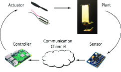
Figure 4: Architecture and components of the prototype.

IV Experimental results

In this section, experimental results for various scenarios are presented. In all the experiments, the sampling time $\delta$ is 0.003 seconds, which is the smallest sampling time that the measurements from our sensors permit. Also we set $\rho_{0}=0.01$, $b=1.00001$, and $J=\frac{M}{\lambda_{1}\rho_{0}}(e^{\lambda_{1}\gamma}-1)+0.1$. In the first set of experiments, we evaluate the performance of the controller for different values of $\gamma$. In Fig. 6, the first row presents the results when $\gamma=0.006$ seconds or two sampling times and the second row presents the results when $\gamma=0.015$ seconds or five sampling times. The first column is the evolution of the absolute value of the state estimation error (50) (red) in time along with the triggering threshold (blue). As the absolute value of this error is greater than or equal to the triggering function, a triggering occurs and the sensor transmits a packet to the controller. However, due to the random delay (upper bounded by $\gamma$) in the communication channel, this error could grow beyond the triggering function. This growth, of course, can become larger as $\gamma$ increases which is shown in the first column of Fig. 6. The first column also shows, more triggering occurred when the channel delay is upper bounded with five sampling times.

The second column in Fig. 6 presents the evolution of the state $x_{1}$ (blue) corresponding to the unstable pole in the diagonalized system (9) and its estimate $\hat{x}_{1}$ (red) in time. The last column shows the evolution of the actual states of the system, namely the angle of the pendulum in radians and its rate of change in radians/sec. It can be seen that $|\phi|$ remains less than $0.2$ radians which ensures the linearization of (3) remains valid and is a good approximation.

We repeat the experiments for different values of $\gamma$ and calculate the sufficient transmission rate using (2). According to the data-rate theorem, to stabilize the plant, the information rate communicated over the channel in data payload and timing should be larger than the entropy rate of the plant [13, 12]. In our experiments, when $\gamma=2\delta$ the timing information is substantial, therefore, the information transmission rate becomes smaller than the entropy rate of the plant which is shown in Fig. 5. Furthermore, according to the theory developed in [22, 23] as $\gamma$ increases, more information has to be sent via data payload for stabilization since larger delay corresponds to more uncertainties about the value of the states at the controller and less timing information.

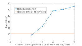
Figure 5: Information transmission rate in experiments compared with the entropy rate of the system. Note that the rate calculated from experiments does not start at zero worst-case delay because the minimum channel delay upper bound is equal to two sampling times (0.006 seconds). The entropy rate of the system is equal to $\lambda_{1}/\ln 2=10.56$ bits/sec while the minimum transmission rate for worst-case delay equal to two sampling time in the experiments is equal to 8.66 bits/sec.

	$M=0.0470$, $\gamma=2\delta=0.006$ sec, $g(t_{s})=1$ bit
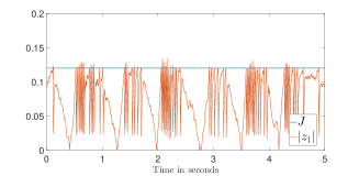
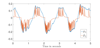
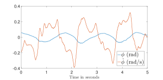
	$M=0.0470$, $\gamma=5\delta=0.015$ sec, $g(t_{s})=7$ bits

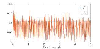
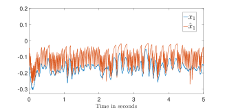
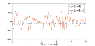
Figure 6: Experimental results for stabilizing the inverted pendulum over a digital channel with random delay upper bounded by two sampling times (first row) and five sampling times (second row). When $\gamma=2\delta$, the packet size is 1 bit and when $\gamma=5\delta$, the packet size becomes 7 bits.

Remark 1

Similar to our analysis in [22], we assume the plant disturbance is random but bounded. In most of our experiments, we successfully stabilized inverted pendulum around its equilibrium point. Disturbances outside the prescribed limits occur rarely, but can still happen occasionally. Assuming that the disturbances are unbounded one might be able to extend the second-moment stability results of [35] to our setup. Similarly, the case where the delay in the communication channel becomes unbounded with a positive probability is another interesting research problem. $\bullet$

V Extension to nonlinear systems

The results developed in [22, 23] are restricted to linear systems, and they can only stabilize the pendulum (3) locally, where the linear approximation is valid. Thus, now we develop a novel event-triggering scheme that encodes information in timing and under appropriate assumptions renders a continuous-time nonlinear system with disturbances ISpS. Clearly, the results of this section compare to the results of [22, 23] are more sophisticated to analyze and implement.

We consider sensor, communication channel, controller system depicted in Fig. 2, and a continuous nonlinear plant

$$\dot{x}=f(x(t),u(t),w(t)),$$ (14)

where $x$, $u$, and $w$ are real numbers representing the plant state, control input, and plant disturbance. Furthermore, we assume that for all time $t\geq 0$

$$|w(t)|\leq M.$$ (15)

As in (49), the controller constructs the state estimation $\hat{x}$, which evolves during the inter-reception times as

$$\dot{\hat{x}}=f(\hat{x}(t),u(t),0)\quad t\in(t_{c}^{k},t_{c}^{k+1}),$$ (16)

starting at $\hat{x}(t_{c}^{k+})$ that is constructed by the controller using information received up to time $t_{c}^{k+}$. The explicit way to construct $\hat{x}(t_{c}^{k+})$ will be explained later in this section (see (34)). As discussed in Appendix -B, we assume the sensor can also calculate the controller’s state estimate $\hat{x}(t)$.

The state estimation error is defined as (50), thus for $t\in(t_{c}^{k},t_{c}^{k+1})$ we have

$$\dot{z}=f(x(t),u(t),w(t))-f(\hat{x}(t),u(t),0).$$ (17)

A triggering occurs at time

$$t_{s}^{k}=k(\alpha+\gamma)$$ (18)

and the sensor transmits a packet $p(t_{s})$ of length $g(t_{s})$ to the controller if

$$|z_{1}(t_{s}^{k})|\geq J,$$ (19)

where $J$ and $\alpha$ are non-negative real numbers, $\gamma$ is the upper bound on the channel delay, $k\in\mathbb{N}$, and $t_{s}^{0}=0$. We choose $g(t_{s})$ such that after decoding we have

$$|z(t_{c}^{k+})|\leq J.$$ (20)

Clearly, the periodic event-triggering scheme (18) and (19) does not exhibit Zeno behavior, meaning that there cannot be infinitely many triggering events in a finite time interval. In fact, we have

$$\Delta^{\prime}_{k}=t_{s}^{k+1}-t_{s}^{k}\geq\alpha+\gamma.$$ (21)

Assumption 1

The dynamic (14) satisfies the Lipschitz property

$$|f(x,u,w)-f(\hat{x},u,0)|\leq L_{x}|x-\hat{x}|+L_{w}|w|,$$ (22)

where $L_{x}>0$, $L_{w}>0$, and

$$|z(t)|=|x(t)-\hat{x}(t)|\leq\Upsilon(\gamma).$$ (23)

Here for all $0\leq\vartheta\leq\gamma$, $\Upsilon(\vartheta)$ is defined as follows

$$\Upsilon(\vartheta):=Je^{L_{x}(\alpha+\gamma+\vartheta)}+\frac{L_{w}M}{L_{x}}\left(e^{L_{x}(\alpha+\gamma+\vartheta)}-1\right).~{}~{}$$ (24)

The reason for choosing the specific value for $\Upsilon(\gamma)$ in (23) will become clear by looking at the following Lemma. If a triggering occurs at time $t_{s}^{k}$, we define

$$\underline{t}^{k}=\mbox{inf}\left\{t\in(t_{s}^{k-1},t_{s}^{k}]~{};~{}|z(t)|=J\right\}.$$ (25)

By continuity of $z$ during the inter-reception time, and using (17) and (20), we see that $\underline{t}^{k}$ is well defined. This definition is used in the next Lemma.

Lemma 1

Consider the plant-sensor-channel-controller model with plant dynamics (14) satisfying Lipschitz property (22), estimator dynamics (16), triggering strategy (18), and (19). Assume $|z(0)|=|x(0)-\hat{x}(0)|<J$ and (20) occurs at all reception times $\{t^{k}_{c}\}_{k\in\mathbb{N}}$. Then for all time $t\in[\underline{t}^{k},t_{c}^{k})$, where $\vartheta=t-t_{s}^{k}$, we have

$$|z(t)|\leq$$ (26)

$$\Upsilon_{w}(\vartheta):=Je^{L_{x}(\alpha+\gamma+\vartheta)}+\frac{L_{w}|w|_{t}}{L_{x}}\left(e^{L_{x}(\alpha+\gamma+\vartheta)}-1\right).$$ (27)

Lem. 1 has two important implications. First, if a triggering event does not occur at $t_{s}^{k}$ for all $t\in(t_{s}^{k-1},t_{s}^{k}]$ we have $|z(t)|\leq J$, hence using (20), under the assumptions of Lem. 1 for all time $t\geq 0$ we have

$$|z(t)|\leq\Upsilon_{w}(\vartheta)\overset{(a)}{\leq}\Upsilon_{w}(\gamma)\overset{(b)}{\leq}\Upsilon(\gamma),$$ (28)

where $(a)$ follows from $\vartheta\leq\gamma$, and $(b)$ follows from (15) and (24). Also, this last inequality explains why we defined the Lipschitz property as (23). The second important implication of Lem. 1 is that for all $k\in\mathbb{N}$ we have

$$z(t_{s}^{k})\in[-\Upsilon(0),\Upsilon(0)].$$ (29)

To construct the packet $p(t_{s})$ of length $g(t_{s})$, we uniformly quantize the interval $[-\Upsilon(0),\Upsilon(0)]$ into $2^{g(t_{s})}$ equal intervals of size $2\gamma(0)/2^{g(t_{s})}$. Once the controller receives the packet, it determines the correct sub-interval and selects its center point as the estimate of $z(t_{s}^{k})$, which is represented by $\bar{z}(t_{s})$. In this case, we have

$$|z(t_{s})-\bar{z}(t_{s})|\leq\Upsilon(0)/2^{g(t_{s})}.$$ (30)

By (50) we have $x(t_{s})=z(t_{s})+\hat{x}(t_{s})$, thus using $\bar{z}(t_{s})$ the controller can construct an estimate of $x(t_{s})$ which we denote by $\bar{x}(t_{s})$ as follows

$$\bar{x}(t_{s})=\bar{z}(t_{s})+\hat{x}(t_{s}).$$ (31)

By (30) we deduce that

$$|\bar{x}(t_{s})-x(t_{s})|\leq\Upsilon(0)/2^{g(t_{s})}.$$ (32)

For all $t\in[t_{s},t_{c}]$ consider the differential equation

$$\dot{\bar{x}}=f(\bar{x}(t),u(t),0)$$ (33)

with initial condition $\bar{x}(t_{s})$ given in (31), and let its solution at time $t_{c}$ be equal to $\hat{x}(t_{c}^{+})$, namely

$$\hat{x}(t_{c}^{+})=\bar{x}(t_{s})+\int_{t_{s}}^{t_{c}}f(\bar{x}(t),u(t),0).$$ (34)

We use the above quantization policy to find a sufficient packet size in the next Theorem.

Theorem 1

Consider the plant-sensor-channel-controller model with plant dynamics (14) with Lipschitz property (22), estimator dynamics (16), triggering strategy (18), and (19). Assume $|z(0)|=|x(0)-\hat{x}(0)|<J$, then there exists a quantization policy that achieves (20) for all reception times $\{t^{k}_{c}\}_{k\in\mathbb{N}}$ with any packet size

$$g(t_{s})\geq\max\left\{0,\log\left(\frac{\Upsilon(0)e^{L_{x}\gamma}}{J-\frac{L_{w}M}{L_{x}}\left(e^{L_{x}\gamma}-1\right)}\right)\right\},$$ (35)

provided

$$J\geq\frac{L_{w}M}{L_{x}}\left(e^{L_{x}\gamma}-1\right).$$ (36)

In the next assumption we restrict the class of nonlinear systems.

Assumption 2

There exists a control policy $u(t)=\mathfrak{U}(\hat{x})=\mathfrak{U}(x-z)$ which renders the dynamics (14) ($\dot{x}=f(x,\mathfrak{U}(x-z),w)$) ISS with respect to $z(t)$ and $w(t)$, that is, there exists $\beta^{\prime}\in\mathcal{KL}$, $\Pi^{\prime}\in\mathcal{K}_{\infty}(0)$, and $\psi^{\prime}\in\mathcal{K}_{\infty}(0)$ such that for all $t\geq 0$

$$|x(t)|\leq\beta^{\prime}\left(|x(0)|,t\right)+\Pi^{\prime}\left(|z|_{t}\right)+\psi^{\prime}\left(|w|_{t}\right).$$ (37)

Corollary 1

Under the assumptions of Thm. 1 and Assumption 2 for any packet size lower bounded as (35) there exists a control policy which renders the dynamics (14) ISpS.

Using (21) the triggering rate, the frequency at which triggering occurs, is trivially upper bounded by $(\alpha+\gamma)^{-1}$. As a result, under assumptions of Corollary 1 we deduce that for any information transmission rate (2)

$$R_{s}\geq\frac{1}{\alpha+\gamma}\max\left\{0,\log\left(\frac{\Upsilon(0)e^{L_{x}\gamma}}{J-\frac{L_{w}M}{L_{x}}\left(e^{L_{x}\gamma}-1\right)}\right)\right\},~{}~{}\,$$ (38)

there exists a control law that renders the dynamic (14) ISpS.

The interested reader can find some additional remarks and simulations for the nonlinear systems in Appendix -F and -G.

VI Future work

On the theoretical side, future work will explore the theory and implementation of multivariate nonlinear system with uncertainty in its parameters. On the practical validation side, we also plan to test the proposed nonlinear scheme on our inverted pendulum prototype.

-A Notation

Throughout the paper, we use the following notation. We represent the set of real, non-negative real, and natural numbers by , ₊, and $\mathbb{N}$, respectively. Base $2$ and natural logarithms are represented by $\log$ and $\ln$ respectively. Vectors are represented by boldface italic letters and matrices are represented by regular and capital boldface letters. We use regular lowercase letters to represent scalars. To represent an element of a vector, we use the vector name accompanied by the element’s index as its subscript. For a function $f:\real\rightarrow{}^{n}$ and $t\in\real$, the right-hand limit of $f$ at $t$ or $\lim_{s\rightarrow t^{+}}f(s)$ is represented by $f(t^{+})$. Also, the nearest integer less (resp. greater) than or equal to $x$ is represented by $\lfloor x\rfloor$ (resp. $\lceil x\rceil$). The remainder after division of $x$ by $y$ is indicated by the modulo function as $\text{mod}(x,y)$ and $\text{sign}(x)$ returns the sign of $x$. For a scalar continuous-time signal $w(t)$, we define $|w|_{t}=\sup_{s\in[0,t]}|w_{1}(s)|$. Finally, to formulate the stability properties, for non-negative constants $d$ and $d^{\prime}$ we define

$$\mathcal{K}(d):=\{f:{}_{\geq 0}\rightarrow{}_{\geq 0}|f~{}\mbox{continuous,}$$ (39)

$$~{}~{}~{}~{}~{}~{}~{}~{}~{}~{}~{}~{}~{}~{}~{}~{}\mbox{strictly increasing, and}~{}f(0)=d\},$$ (40)

$$\mathcal{K_{\infty}}(d):=\{f\in\mathcal{K}(d)|f~{}\mbox{unbounded}\},$$ (41)

$$\mathcal{K}_{\infty}^{2}(0,d^{\prime}):=\{f:{}_{\geq 0}\times{}_{\geq 0}\rightarrow{}_{\geq 0}|$$ (42)

$$~{}~{}~{}~{}~{}\forall t\geq 0,f(.,t)\in\mathcal{K}_{\infty}(0),~{}\mbox{and}~{}\forall r>0~{}f(r,.)\in\mathcal{K}_{\infty}(d^{\prime})\}$$ (43)

$$\mathcal{L}:=\{f:{}_{\geq 0}\rightarrow{}_{\geq 0}|f~{}\mbox{continuous,}$$ (44)

$$~{}~{}~{}~{}~{}\mbox{strictly decreasing, and}~{}\lim_{s\rightarrow\infty}f(s)=0\},$$ (45)

$$\mathcal{KL}:=\{f:{}_{\geq 0}\times{}_{\geq 0}\rightarrow{}_{\geq 0}|f~{}\mbox{continuous,}$$ (46)

$$~{}~{}~{}~{}~{}\forall t\geq 0,f(.,t)\in\mathcal{K}(0),~{}\mbox{and}~{}\forall r>0~{}f(r,.)\in\mathcal{L}\}.$$ (47)

-B Event-triggering control design

We start with a brief description of the event-triggered control approach in our previous work [22, 23] that achieves ISpS for the first coordinate of the dynamics (9). We have

$$\dot{x}_{1}=\lambda_{1}x_{1}(t)+b_{1}u(t)+w_{1}(t).$$ (48)

At the controller, the estimated state is represented by $\hat{x}_{1}$ and evolves during the inter-reception times as

$$\dot{\hat{x}}_{1}(t)=\lambda_{1}\hat{x}_{1}(t)+b_{1}u(t),\quad t\in(t_{c}^{k},t_{c}^{k+1}),$$ (49)

starting at $\hat{x}_{1}(t_{c}^{k+})$, as the estimate of the state at the controller is updated with the information received up to time $t_{c}^{k+}$. $\hat{x}_{1}(t_{c}^{k+})$ is found by decoding the received packet, as explained later in this section. We assume that the sensor can also construct the estimate $\hat{x}_{1}(t)$ generated by the controller.

Remark 2

As shown in [22, 23], if the sensor has causal knowledge of the delay in the communication channel, it can use $\hat{x}(0)$ to compute $\hat{x}(t)$ at all times $t$. This causal knowledge can be obtained without assuming an additional communication channel in the feedback loop via “acknowledgment through the control input” [36]. $\bullet$

For the unstable coordinate in (9), the state estimation error is defined as

$$z_{1}(t)=x_{1}(t)-\hat{x}_{1}(t).$$ (50)

This error is used by the sensor to determine the triggering events.

We define the triggering events as follows: for $J\geq 0$, a triggering occurs, and the sensor transmits a packet to the controller at time $t_{s}^{k+1}\geq 0$ when

$$|z_{1}(t_{s}^{k+1})|=J,$$ (51)

where $t_{c}^{k}\leq t_{s}^{k+1}$ for $k\in\mathbb{N}$ and $t_{s}^{1}\geq 0$. Thus, a new transmission occurs only if the previous packets have been already delivered to the controller.

Using (51), at each triggering event, the sensor transmits the packet $p(t_{s})$ of size $g(t_{s})$ bits to the controller which contains the data payload and carries the timing information. The details of our quantization policy to encode data payload into packet $p(t_{s})$ is discussed in our previous work [22, 23]. Using the data payload and the timing of the packet $p(t_{s})$ the controller estimates $z_{1}(t_{c})$ as follows

$$\bar{z}_{1}(t_{c})=\text{sign}(z_{1}(t_{s}))Je^{\lambda_{1}(t_{c}-q(t_{s}))},$$ (52)

where $q(t_{s})$ is the best estimate of $t_{s}$ constructed at the controller after reception of the packet $p(t_{s})$.

To update the estimate of the state after decoding the packet, we define the following jump strategy

$$\hat{x}_{1}(t_{c}^{+})=\bar{z}_{1}(t_{c})+\hat{x}_{1}(t_{c}).$$ (53)

For a given design parameter $0<\rho_{0}<1$, the packet size

$$g(t_{s})=\max\left\{1,\left\lceil 1+\log\frac{\lambda_{1}b\gamma}{\ln(1+\frac{\rho_{0}-(M/J\lambda_{1})(e^{\lambda_{1}\gamma}-1)}{e^{\lambda_{1}\gamma}})}\right\rceil\right\},$$ (54)

ensures that

$$|z_{1}(t_{c}^{k+})|=|z_{1}(t_{c}^{k})-\bar{z}_{1}(t_{c}^{k})|\leq\rho_{0}J,$$ (55)

at all reception times $\{t_{c}^{k}\}_{k\in\mathbb{N}}$ inside the closed interval $[t_{s}^{k},t_{s}^{k}+\gamma]$, provided that $J>\frac{M}{\lambda_{1}\rho_{0}}(e^{\lambda_{1}\gamma}-1)$ and $|z_{1}(0)|\leq J$. It then follows that for all $t$ we have

$$|z_{1}(t)|\leq Je^{\lambda_{1}\gamma}+\frac{M}{\lambda_{1}}\left(e^{\lambda_{1}\gamma}-1\right).$$ (56)

The proof and derivation of (54), (55), and (56) can be found in our previous work [22, 23].

We set the control input to be $u(t)=-\textbf{K}\hat{\boldsymbol{x}}(t)$. In our example, we have $\textbf{K}=(225,11)$, and K is chosen such that $(\textbf{A}-\textbf{B}\textbf{K})$ is Hurwitz. Here, $\hat{x}_{1}(t)$ is generated based on (49) and jump strategy (53). Since $\lambda_{2}<0$, the controller does not need any update from the sensor to construct $\hat{x}_{2}(t)$. Therefore, as mentioned in [22], using (56), one can prove that the plant (7) is ISpS. We can then conclude that as long as the linear approximation holds, the nonlinear plant (3) is also ISpS.

In [22, 23] we have also shown that the proposed event-triggered scheme does not exhibit “Zeno behavior,” meaning that there cannot be infinitely many triggering events in a finite time interval. In fact, the time between consecutive triggers is uniformly lower bounded as follow

$$\Delta^{\prime}_{k}=t_{s}^{k+1}-t_{s}^{k}\geq\frac{1}{\lambda_{1}}\ln\Big{(}\frac{J+\frac{M}{\lambda_{1}}}{\rho_{0}J+\frac{M}{\lambda_{1}}}\Big{)}.$$ (57)

-C Proof of Lemma 1

Proof:

For all time $t\in[\underline{t}^{k},t_{c}^{k})$ the state estimation error evolves according to (17) with the initial condition $z(\underline{t}^{k})=J$, where $\underline{t}^{k}$ is defined as (25). Thus, for all $t\in[\underline{t}^{k},t_{c}^{k})$

$$|z(t)|\leq Je^{L_{x}(t-\underline{t}^{k})}+L_{w}\int_{\underline{t}^{k}}^{t}|w(t)e^{L_{x}(t-\underline{t}^{k})}|dt$$ (58a)

$$\leq Je^{L_{x}(t-\underline{t}^{k})}+\frac{L_{w}|w|_{t}}{L_{x}}\left(e^{L_{x}(t-\underline{t}^{k})}-1\right)$$ (58b)

$$=Je^{L_{x}(t-t_{s}+t_{s}-\underline{t}^{k})}+\frac{L_{w}|w|_{t}}{L_{x}}\left(e^{L_{x}(t-t_{s}+t_{s}-\underline{t}^{k})}-1\right)$$ (58c)

$$\leq Je^{L_{x}(\vartheta+\alpha+\gamma)}+\frac{L_{w}|w|_{t}}{L_{x}}\left(e^{L_{x}(\vartheta+\alpha+\gamma)}-1\right),$$ (58d)

where (58a) follows from the Lipschitz property (22) and Gronwall-Bellman inequality, as $\underline{t}^{k}\in(t_{s}^{k-1},t_{s}^{k}]$ we have $t_{s}^{k}-\underline{t}^{k}\leq\alpha+\gamma$ and (58d) follows. ∎

-D Proof of Theorem 1

Proof:

For all $t\in[t_{s},t_{c}]$ we have

$$|x(t)-\bar{x}(t)|=\left|x(t_{s})-\bar{x}(t_{s})\right|+$$ (59a)

$$\left|\int_{t_{s}}^{t}f(x,u,w)dt-\int_{t_{s}}^{t}f(\bar{x},u,0)dt\right|\leq$$ (59b)

$$|x(t_{s})-\bar{x}(t_{s})|+\int_{t_{s}}^{t}\left(L_{x}|x-\bar{x}|+L_{w}|w|\right)dt\leq$$ (59c)

$$|x(t_{s})-\bar{x}(t_{s})|e^{L_{x}(t-t_{s})}+$$ (59d)

$$~{}~{}~{}~{}~{}~{}~{}~{}~{}~{}~{}~{}~{}~{}L_{w}\int_{t_{s}}^{t}|w(t)e^{L_{x}(t-t_{s})}|dt\leq$$ (59e)

$$|x(t_{s})-\bar{x}(t_{s})|e^{L_{x}(t-t_{s})}+\frac{L_{w}M}{L_{x}}\left(e^{L_{x}(t-t_{s})}-1\right)$$ (59f)

where we used (14) and (33) along the triangle inequality to arrive at (59b), (59c) follows from Lipschitz property (22), and (59e) follows from solving the linear differential equation $\dot{x}(t)-\dot{\bar{x}}(t)=L_{x}(x-\bar{x})+L_{w}w$ with initial condition $x(t_{s})-\bar{x}(t_{s})$ (see Gronwall-Bellman inequality), and (59f) follows from (15).

Using (1), (32), (34) and (59) we deduce

$$|z(t_{c}^{+})|=|x(t_{c})-\hat{x}(t_{c}^{+})|\leq$$ (60)

$$~{}~{}~{}~{}~{}~{}~{}~{}~{}~{}~{}~{}~{}~{}~{}~{}~{}~{}~{}~{}\frac{\Upsilon(0)}{2^{g(t_{s})}}e^{L_{x}\gamma}+\frac{L_{w}M}{L_{x}}\left(e^{L_{x}\gamma}-1\right).$$ (61)

Consequently,

$$\frac{\Upsilon(0)}{2^{g(t_{s})}}e^{L_{x}\gamma}+\frac{L_{w}M}{L_{x}}\left(e^{L_{x}\gamma}-1\right)\leq J$$ (62)

suffices to ensure (20) at all reception time. Using (36), (62) is equivalent to

$$2^{g(t_{s})}\geq\frac{\Upsilon(0)e^{L_{x}\gamma}}{J-\frac{L_{w}M}{L_{x}}\left(e^{L_{x}\gamma}-1\right)}.$$ (63)

The result now follows by noticing the packet size should be no-negative. ∎

-E Proof of Corollary 1

Proof:

Thm. 1 states that with any packet size lower bounded as (35) there exists a quantization policy that achieves (20) for all reception times $\{t^{k}_{c}\}_{k\in\mathbb{N}}$. Thus using Lem. 1 and (28) we deduce for all time $t\geq 0$ we have

$$|z(t)|\leq\Upsilon_{w}(\gamma),$$ (64)

where $\Upsilon_{w}(\gamma)$ is defined as (26). Consequently, for all time $t\geq 0$, $|z(t)|$ is upper bounded by summation of a $\mathcal{K}_{\infty}(d)$ function of $\gamma$ with $d=Je^{L_{x}\alpha}$ and a $\mathcal{K}_{\infty}^{2}(0,d^{\prime})$ function of $|w|_{t}$ and $\gamma$ with $d^{\prime}=(e^{L_{x}\alpha}-1)L_{w}M/L_{x}$. Therefore, using Assumption 2 the result follows. ∎

-F Additional remarks about nonlinear systems

$M=0.1$, $\gamma=0.1$ sec, $g(t_{s})=3$ bit	$M=0.1$, $\gamma=0.99$ sec, $g(t_{s})=15$ bit

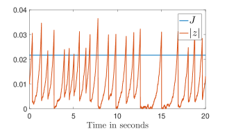
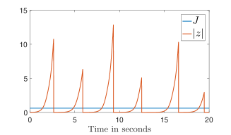
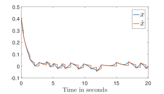
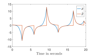
Figure 7: Simulation results for stabilization of the plant (66). We used the following parameters for the simulation: sampling time $\delta=0.005$, simulation time $T=20$, $u(t)=-4\hat{x}(t)$, $\alpha=0.01$, packet size (65), and triggering threshhold $J=(e^{3\gamma}-1)M/3+0.01$.

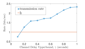
Figure 8: Information transmission rate in simulations compared to the $\underline{h}$ (68). We used the following parameters for the simulation: sampling time $\delta=0.01$ seconds, simulation time $T=100$ seconds, $u(t)=-2\hat{x}(t)$, $z(0)=0.01$, $M=0.05$, $\alpha=0.01$, packet size (65), and triggering threshhold $J=(e^{3\gamma}-1)M/3+0.05$. Note that the rate calculated from simulations can not start at $\gamma=0$ because the minimum channel delay upper bound is equal to two sampling time.

Here, we discuss some additional remarks about the nonlinear systems results presented in Sec. V.

Remark 3

Unlike the linear case, a closed form solution of (17) is not known in general. Consequently, to simplify the encoding process, we use the periodic event-triggering scheme (18) and (19) (cf. [37]), which is different from the continues time event-triggering scheme (51) where a triggering could occur at any time $t_{s}^{k}\geq 0$. $\bullet$

Remark 4

Although Assumption 2 is restrictive, it is widely used in control of nonlinear systems under communication constraint [25, 38, 27]. An exception is the work [38] which eliminated this assumption for systems without disturbances. An alternative ISS assumption which centers around state estimation $\hat{x}$ is proposed in [27] where the evolution of state estimation $\hat{x}$ is described by an impulsive system [39]. As in our event-triggering design the behavior of the state estimation $\hat{x}$ is described with an impulsive system (16) and (34), the study of this alternative ISS assumption for our setup with a digital communication channel with bounded but unknown delay is an interesting research venue. $\bullet$

Remark 5

The lower bound given on the packet size in (35) might not be a natural number in general. This lower bound is used to properly bound the information transmission rate (2) in (38). In addition, the lower bound (35) might be zero. When $g(t_{s})=0$ there is no need to put any data payload in the packet and the plant can be stabilized using only timing information. However, in this case the sensor still needs to inform the controller about the occurrence of a triggering event. Consequently, when $g(t_{s})=0$ is sufficient, the sensor can stabilize the system by transmitting a fixed symbol from a unitary alphabet to the controller (see [13]). In practice, the packet size should be a natural number or zero, so if we do not want to use the fixed symbol from a unitary alphabet, as in (54), the packet size

$$g(t_{s})=\max\left\{1,\left\lceil\log\left(\frac{\Upsilon(0)e^{L_{x}\gamma}}{J-\frac{L_{w}M}{L_{x}}\left(e^{L_{x}\gamma}-1\right)}\right)\right\rceil\right\},$$ (65)

is sufficient for stabilization. $\bullet$

Remark 6

As we used the trivial upper bound on the triggering rate $(\alpha+\gamma)^{-1}$ to deduce the bound (38), this upper bound on $R_{s}$ might be too conservative in general. $\bullet$

Remark 7

When $\gamma=M=0$, the data-rate theorem[12, 22, 23] states that the rate at which the controller receives information should be at least as large as the intrinsic entropy rate of the plant defined in [26]. In our design, we can supply this information only using the implicit timing information in the triggering events. In fact, when $\alpha\rightarrow 0$ the periodic event-triggering control schemes (18) and (19) become equivalent to the continuous time event-triggering policy (51). In this case, in a triggering time $t_{s}$ the controller can discover the exact value of $x(t_{s})$ using equation $x(t_{s})=\hat{x}(t_{s})\pm J$ by receiving a single bit corresponding to the sign of $z(t_{s})$. As there is no system disturbance, the controller then can track $x(t)$ using (16) after a single triggering time, and $R_{s}$ (2) will be arbitrarily small. $\bullet$

-G Simulations for nonlinear systems

This section presents simulation results validating the proposed nonlinear scheme. While our analysis is for continuous-time plants, we perform the simulations in discrete time with a small sampling time $\delta$. In this case, as discussed in Sec. III, the minimum upper bound for the channel delay is equal to two sampling times. We illustrate the execution of our design for the system

$$\dot{x}=f(x(t),u(t),w(t))=2x(t)+\sin(x(t))+u(t)+w(t).$$ (66)

During inter-reception time, state estimation is defined according to (16). Thus, using (17), for $t\in(t_{c}^{k},t_{c}^{k+1})$ we deduce

$$\dot{z}(t)=2z(t)+\sin x-\sin\hat{x}+w(t).$$ (67)

Since $|\sin x-\sin\hat{x}|\leq|x-\hat{x}|$, the dynamics (66) satisfies the Lipschitz property (22) with $L_{x}=3$, $L_{w}=1$ for all $|z(t)|\in\mathbb{R}_{\geq 0}$.

A set of two simulations are carried out for different values of $\gamma$ and $M$. Each column in Fig. 7 presents one set of simulation. The first row shows the triggering threshold $J$ and the absolute value of the state estimation error $|z(t)|$. If the absolute value of this error is equal to $J$ during the period $\alpha+\gamma$, the sensor transmits a packet at the end of this period, and the jumping strategy (34) adjusts $\hat{x}$ at the reception time to ensure the plant is ISpS.

Note that the amount this error exceeds the triggering function depends on the random channel delay, upper bounded by $\gamma$. The second row of Fig. 7 presents the evolution of the state (66) and its estimation (16). As expected, when $\gamma$ increases, while the plant remains ISpS the controller performance deteriorate significantly.

As discussed in Sec. IV, according to the data-rate theorem, to stabilize the plant, the information rate communicated over the channel in data payload and timing should be larger than the entropy rate of the plant [13, 12]. Using [26] the entropy rate of the plant (66) at point $x^{*}$ is equal to $h(x^{*})=\partial f/\partial x|_{x=x^{*}}=2+\cos(x^{*}(t))$. Thus, for any value of the state, the information accessible to the controller about the plant or the information rate communicated over the channel in data payload and timing, should be larger than

$$h(x)\geq\underline{h}=1.$$ (68)

Fig. 8 presents the simulation of information transmission rate versus the delay upper bound $\gamma$ in the communication channel to render (14) ISpS. It can be seen that for small values of $\gamma$, the plant is ISpS with an information transmission rate smaller than the one prescribed by the data-rate theorem. Furthermore, as $\gamma$ increases, more information has to be sent via data payload for stabilization since larger delay corresponds to more uncertainties about the value of the states at the controller and less timing information.

References

- [1] P. Tabuada, “Event-triggered real-time scheduling of stabilizing control tasks,” IEEE Tran. Auto. Cont., vol. 52, no. 9, pp. 1680–1685, 2007.
- [2] X. Wang and M. D. Lemmon, “Event-triggering in distributed networked control systems,” IEEE Tran. Auto. Cont., vol. 56, no. 3, pp. 586–601, 2011.
- [3] W. P. M. H. Heemels, K. H. Johansson, and P. Tabuada, “An introduction to event-triggered and self-triggered control,” in Proc. IEEE Conf. Decis. Cont., 2012, pp. 3270–3285.
- [4] J. Pearson, J. P. Hespanha, and D. Liberzon, “Control with minimal cost-per-symbol encoding and quasi-optimality of event-based encoders,” IEEE Tran. Auto. Cont., vol. 62, no. 5, pp. 2286–2301, 2017.
- [5] P. Tallapragada and N. Chopra, “On event triggered tracking for nonlinear systems,” IEEE Tran. Auto. Cont., vol. 58, no. 9, pp. 2343–2348, 2013.
- [6] R. Postoyan, P. Tabuada, D. Nešić, and A. Anta, “A framework for the event-triggered stabilization of nonlinear systems,” IEEE Tran. Auto. Cont., vol. 60, no. 4, pp. 982–996, 2015.
- [7] A. Girard, “Dynamic triggering mechanisms for event-triggered control,” IEEE Tran. Auto. Cont., vol. 60, no. 7, pp. 1992–1997, 2015.
- [8] H. Yildiz, Y. Su, A. Khina, and B. Hassibi, “Event-triggered stochastic control via constrained quantization,” in Proc. IEEE Data Comp. Conf. (DCC), 2019, pp. 612–612.
- [9] S. Linsenmayer, H. Ishii, and F. Allgöwer, “Containability with event-based sampling for scalar systems with time-varying delay and uncertainty,” IEEE Cont. Sys. Let., vol. 2, no. 4, pp. 725–730, 2018.
- [10] A. Seuret, C. Prieur, S. Tarbouriech, and L. Zaccarian, “LQ-based event-triggered controller co-design for saturated linear systems,” Automatica, vol. 74, pp. 47–54, 2016.
- [11] B. A. Khashooei, D. J. Antunes, and W. Heemels, “A consistent threshold-based policy for event-triggered control,” IEEE Cont. Sys. Let., vol. 2, no. 3, 2018.
- [12] M. J. Khojasteh, P. Tallapragada, J. Cortés, and M. Franceschetti, “Time-triggering versus event-triggering control over communication channels,” in Proc. IEEE Conf. Decis. Cont., 2017, pp. 5432–5437.
- [13] M. J. Khojasteh, M. Franceschetti, and G. Ranade, “Stabilizing a linear system using phone calls,” in Proc. Euro. Cont. Conf. IEEE, 2019, pp. 2856–2861.
- [14] M. J. Khojasteh, P. Tallapragada, J. Cortés, and M. Franceschetti, “The value of timing information in event-triggered control,” IEEE Tran. Auto. Cont., 2020.
- [15] B. G. N. Nair, F. Fagnani, S. Zampieri, and R. J. Evans, “Feedback control under data rate constraints: An overview,” Proceedings of the IEEE, vol. 95, no. 1, pp. 108–137, 2007.
- [16] S. Tatikonda and S. Mitter, “Control under communication constraints,” IEEE Tran. Auto. Cont., vol. 49, no. 7, pp. 1056–1068, 2004.
- [17] A. Khina, E. R. Garding, G. M. Pettersson, V. Kostina, and B. Hassibi, “Control over gaussian channels with and without source-channel separation,” IEEE Tran. Auto. Cont., 2019.
- [18] V. Kostina and B. Hassibi, “Rate-cost tradeoffs in control,” IEEE Tran. Auto. Cont., 2019.
- [19] M. Franceschetti and P. Minero, “Elements of information theory for networked control systems,” in Info. and Cont. in Net. Springer, 2014, pp. 3–37.
- [20] N. C. Martins, M. A. Dahleh, and N. Elia, “Feedback stabilization of uncertain systems in the presence of a direct link,” IEEE Tran. Auto. Cont., vol. 51, no. 3, pp. 438–447, 2006.
- [21] J. Hespanha, A. Ortega, and L. Vasudevan, “Towards the control of linear systems with minimum bit-rate,” in Proc. 15th Int. Symp. Math. Theory Netw. Syst., 2002.
- [22] M. J. Khojasteh, M. Hedayatpour, J. Cortés, and M. Franceschetti, “Event-triggered stabilization of disturbed linear systems over digital channels,” in Ann. Conf. on Inf. Sci. and Sys. IEEE, 2018, pp. 1–6.
- [23] M. J. Khojasteh, M. Hedayatpour, J. Cortes, and M. Franceschetti, “Event-triggered stabilization over digital channels of linear systems with disturbances,” arXiv preprint arXiv:1805.01969, 2018.
- [24] Z.-P. Jiang, A. R. Teel, and L. Praly, “Small-gain theorem for ISS systems and applications,” Math. of Cont., Sig. and Sys., vol. 7, no. 2, pp. 95–120, 1994.
- [25] Y. Sharon and D. Liberzon, “Input to state stabilizing controller for systems with coarse quantization,” IEEE Tran. Auto. Cont., vol. 57, no. 4, pp. 830–844, 2012.
- [26] G. N. Nair, R. J. Evans, I. M. Mareels, and W. Moran, “Topological feedback entropy and nonlinear stabilization,” IEEE Tran. Auto. Cont., vol. 49, no. 9, pp. 1585–1597, 2004.
- [27] D. Liberzon and J. P. Hespanha, “Stabilization of nonlinear systems with limited information feedback,” IEEE Tran. Auto. Cont., vol. 50, no. 6, pp. 910–915, 2005.
- [28] C. De Persis, “n-bit stabilization of n-dimensional nonlinear systems in feedforward form,” IEEE Tran. Auto. Cont., vol. 50, no. 3, pp. 299–311, 2005.
- [29] D. Liberzon, “On stabilization of linear systems with limited information,” IEEE Tran. Auto. Cont., vol. 48, no. 2, pp. 304–307, 2003.
- [30] V. Sanjaroon, A. Farhadi, A. S. Motahari, and B. H. Khalaj, “Estimation of nonlinear dynamic systems over communication channels,” IEEE Tran. Auto. Cont., vol. 63, no. 9, pp. 3024–3031, 2018.
- [31] E. D. Sontag, “Input to state stability: Basic concepts and results,” in Nonlin. and Opt. Cont. The. Springer, 2008, pp. 163–220.
- [32] R. Dou, J. Chen, F. Li, S. Wang, and Q. Ling, “A sufficient bit rate condition for stabilizing a scalar continuous-time nonlinear system with bounded processing delay,” in 37th Chin. Cont. Conf. IEEE, 2018, pp. 6265–6270.
- [33] A. Tanwani and A. Teel, “Stabilization with event-driven controllers over a digital communication channel with random transmissions,” in Proc. IEEE Conf. Decis. Cont., 2017, pp. 6063–6068.
- [34] Z. Music, F. Molinari, S. Gallenmüller, O. Ayan, S. Zoppi, W. Kellerer, G. Carle, T. Seel, and J. Raisch, “Design of a networked controller for a two-wheeled inverted pendulum robot,” arXiv preprint arXiv:1812.03071, 2018.
- [35] G. N. Nair and R. J. Evans, “Stabilizability of stochastic linear systems with finite feedback data rates,” SIAM Jour. on Cont. and Opt., vol. 43, no. 2, pp. 413–436, 2004.
- [36] S. Tatikonda and S. Mitter, “Control over noisy channels,” IEEE Tran. Auto. Cont., vol. 49, no. 7, pp. 1196–1201, 2004.
- [37] W. H. Heemels, M. Donkers, and A. R. Teel, “Periodic event-triggered control for linear systems,” IEEE Tran. Auto. Cont., vol. 58, no. 4, pp. 847–861, 2013.
- [38] C. De Persis and A. Isidori, “Stabilizability by state feedback implies stabilizability by encoded state feedback,” Sys. & cont. let., vol. 53, no. 3-4, pp. 249–258, 2004.
- [39] J. P. Hespanha, D. Liberzon, and A. R. Teel, “Lyapunov conditions for input-to-state stability of impulsive systems,” Automatica, vol. 44, no. 11, pp. 2735–2744, 2008.