Multiphoton resonances in nitrogen-vacancy defects in diamond

Abstract

Dense ensembles of nitrogen vacancy (NV) centers in diamond are of interest for various applications including magnetometry, masers, hyperpolarization and quantum memory. All of the applications above may benefit from a non-linear response of the ensemble, and hence multiphoton processes are of importance. We study an enhancement of the NV ensemble multiphoton response due to coupling to a superconducting cavity or to an ensemble of Nitrogen 14 substitutional defects (P1). In the latter case, the increased NV sensitivity allowed us to probe the P1 hyperfine splitting. As an example of an application, an increased responsivity to magnetic field is demonstrated.

I Introduction

A two level system (TLS) is perhaps the most extreme manifestation of nonlinear response. Systems composed of TLSs and other elements exhibit a variety of nonlinear dynamical effects including multi-photon resonances (MPR) Shirley (1965); Berns et al. (2006); Tycko and Opella (1987); Faisal (2013), frequency mixing Childress and McIntyre (2010); Chen et al. (2018); Mamin et al. (2014), fluorescence Mollow (1973); Freedhoff and Quang (1994), dynamical instabilities WEBER (1959); Armen and Mabuchi (2006), suppression of tunneling Grossmann et al. (1991); Lignier et al. (2007) and breakdown of the rotating wave approximation Fuchs et al. (2009).

Here we study nonlinear response of an ensemble of nitrogen-vacancy (NV) defects in diamond Doherty et al. (2013). Two mechanisms that allow the enhancement of MPR are explored. The first one is based on an electromagnetic cavity mode that is coupled to the spin ensemble Zhu et al. (2011); Kubo et al. (2010, 2011); Amsüss et al. (2011); Schuster et al. (2010); Sandner et al. (2012); Grezes et al. (2014); Alfasi et al. (2018). The second one is attributed to hyperfine splitting Álvarez et al. (2015) of P1 defects Kamp et al. (2018); Sushkov et al. (2014); Belthangady et al. (2013) and their dipolar coupling to the negatively charged NV defects ($\text{NV}^{-}$).

The $\text{NV}^{-}$ defect has a spin triplet ground state Doherty et al. (2012) having relatively long coherence time Balasubramanian et al. (2009). The NV^- spin state can be initiated via the process of optically-induced spin polarization (OISP) Robledo et al. (2011); Redman et al. (1991) and can be measured using the technique of optical detection of magnetic resonance (ODMR) Shin et al. (2012); Chapman and Plakhotnik (2011); Gruber et al. (1997). These properties facilitate a variety of applications including magnetometry Maze et al. (2008); Acosta et al. (2010); Balasubramanian et al. (2008); Wolf et al. (2015); Mamin et al. (2013); Pelliccione et al. (2016); Rondin et al. (2013); Sushkov et al. (2014), sensing Acosta et al. (2010); Dolde et al. (2011); Balasubramanian et al. (2009); Jelezko et al. (2004) and quantum information processing Maurer et al. (2012); Cai et al. (2012).

Dipolar coupling between NV^- and other spin species in diamond gives rise to intriguing effects including hyperpolarization Takahashi et al. (2008); Fischer et al. (2013a, b); Wang et al. (2013) and cross-relaxation Solomon (1955); Belthangady et al. (2013); Loretz et al. (2017), and can be exploited for optical detection of spin defects in diamond other than NV^- Simanovskaia et al. (2013); Kamp et al. (2018); Clevenson et al. (2016); Wang et al. (2014); Hall et al. (2016); Purser et al. (2018); Alfasi et al. (2019).

The process of cross-polarization between NV^- and P1 defects plays an important role in the MPR mechanism. In general, the efficiency of cross polarization depends on the rate of a competing effect of thermal polarization, which is characterized by the longitudinal spin relaxation rate. At cryogenic temperatures the thermal polarization rate can be significantly reduced, and consequently the efficiently of cross-polarization is enhanced.

II Low Magnetic Field ODMR

A spiral resonator Kurter et al. (2011) made of $500\operatorname{nm}/10\operatorname{nm}$ thick Niobium/Aluminum with the inner radius of $0.7\operatorname{mm}$ and line width and spacing of $20\operatorname{\mu m}$ is fabricated on a Sapphire substrate. Type Ib [110] diamond is irradiated with $2.8\operatorname{MeV}$ electrons at a doze of $8\times 10^{18}\operatorname{e/cm}^{2}$, annealed for $2$ hours at $900\operatorname{C}^{\circ}$ and acid cleaned. The samples assembly (see Fig. 1) is placed at a cryostat with base temperature of $3.6\operatorname{K}$ and mechanically aligned along the magnetic field of an external superconducting solenoid. The photoluminescence light passes through an array of filters and is collected by a photodiode. A microwave synthesizer is connected directly to a loop antenna (shortened end of a coaxial cable) mounted below the sapphire substrate, and the signal amplitude is $100\%$ modulated with a low frequency sine wave. The same wave is used for the photodiode signal demodulation by a lock-in amplifier. Microwave reflection measurements of the resonator yield resonance frequency $\omega_{\mathrm{c}}=2\pi\times 276\operatorname{MHz}$, unloaded quality factor $Q=96$ and critical temperature $T_{\text{c}}=7\operatorname{K}$. The rather low $Q$ might be explained by the proximity to irradiated diamond. The coupling coefficient $g$ between the resonator and the $\text{NV}^{-}$ ensemble is given by Alfasi et al. (2018)

$$g^{2}=\frac{\gamma_{\mathrm{e}}^{2}\mu_{0}\hbar\omega_{\mathrm{c}}\int d\mathbf{r}n_{\mathrm{S}}P_{z}\left|\mathbf{B}_{\mathrm{c}}\right|^{2}\sin^{2}\varphi}{\int d\mathbf{r}{}\left|\mathbf{B}_{\mathrm{c}}\right|^{2}},$$ (1)

where $P_{z}\approx 0.15$ Alfasi et al. (2019) is the spin polarization, $n_{\mathrm{S}}$ is the NV^- ensemble number density, $\varphi$ is the angle between the NV^- axis and the cavity magnetic field $\mathbf{B}_{\mathrm{c}}$, $\mu_{0}$ is the free space permeability and $\gamma_{\mathrm{e}}=2\pi\times 28.03\operatorname{GHz}\operatorname{T}^{-1}$ is the electron spin gyromagnetic ratio. Assuming constant $P_{z}$ throughout the diamond, $g$ is readily calculated by means of numerical simulation [see Fig.1(b)] to be $g=8\operatorname{MHz}$.

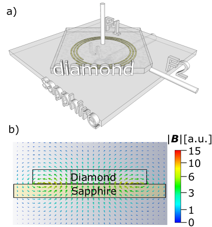
Figure 1: (a) Experimental setup. The diamond is glued on the top of the spiral resonator, and two multimode optical fibers F1 and F2 are attached to the diamond top and side faces correspondingly. A $532\operatorname{nm}$ wavelength laser is introduced from one of the fibers, and the photoluminescence is collected from the other, providing a geometrical filtering of the laser light. A microwave loop antenna is placed below the Sapphire at a location optimizing the resonator coupling. (b) Numerical simulation CST of America (2019) of the spiral fundamental mode magnetic field distribution.

ODMR as a function of magnetic field and frequency is shown in Fig. 2. The dotted lines in Fig. 2 are calculated by numerically diagonalizing the NV^- ground state spin triplet Hamiltonian, which is given by Ovartchaiyapong et al. (2014); MacQuarrie et al. (2013)

$$\frac{\mathcal{H}_{\mathrm{NV}}}{\hbar}=\frac{DS_{z}^{2}}{\hbar^{2}}+\frac{E\left(S_{+}^{2}+S_{-}^{2}\right)}{2\hbar^{2}}-\frac{\gamma_{\mathrm{e}}\mathbf{B}\cdot\mathbf{S}}{\hbar}\;,$$ (2)

where $\mathbf{S}=\left(S_{x},S_{y},S_{z}\right)$ is a vector spin $S=1$ operator, the raising $S_{+}$ and lowering $S_{-}$ operators are defined by $S_{\pm}=S_{x}\pm iS_{y}$, the zero field splitting induced by spin-spin interaction $D$ is given by $D=2\pi\times 2.87\operatorname{GHz}$, the strain-induced splitting $E$ is about $2\pi\times 10\operatorname{MHz}$ for our sample and $\mathbf{B}$ is the externally applied magnetic field. The field $\mathbf{B}$ has two contributions $\mathbf{B}=\mathbf{B}_{\mathrm{S}}+\mathbf{B}_{\mathrm{L}}$, where $\mathbf{B}_{\mathrm{S}}$ ($\mathbf{B}_{\mathrm{L}}$) is the stationary (alternating) field generated by the solenoid (the loop antenna) and is nearly parallel to the lattice direction $\left[111\right]$ ($\left[1\bar{1}0\right]$).

In a single crystal diamond the NV centers have four different possible orientations. When hyperfine interaction is disregarded each orientation gives rise to a pair of angular resonance frequencies $\omega_{\pm}$, corresponding to the transitions between the spin state with magnetic quantum number $0$ and the spin state with magnetic quantum number $\pm 1$. The dotted line in Fig. 2 having the smallest (largest) frequency for any given magnetic field corresponds to the angular frequency $\omega_{-}$ ($\omega_{+}$) of the NV^- defects having axis in the $\left[111\right]$ lattice direction. The other two dotted lines represent the resonances due to the unparallel NV^- defects having axis in the lattice directions $\left[\bar{1}11\right]$, $\left[1\bar{1}1\right]$ or $\left[11\bar{1}\right]$.

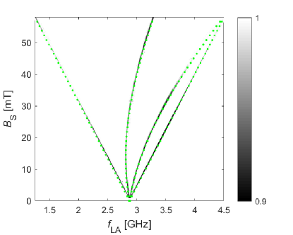
Figure 2: Low magnetic field ODMR. The overlaid green dotted lines are calculated by diagonalizing the NV^- spin Hamiltonian (2). The two nearly straight diagonal curves (leftmost and rightmost) correspond to the NV axis vector nearly parallel to the magnetic field, while the two remaining curves in the middle - to the nearly degenerate three other possible orientations of the NV axis vectors.

III Near the Level Anti Crossing

Let $\omega_{\mathrm{a}}$ denote the angular frequency $\omega_{-}$ corresponding to the NV^- defects having axis in the $\left[111\right]$ lattice direction. Consider the case where the magnitude $B_{\mathrm{S}}$ of the solenoid field $\mathbf{B}_{\mathrm{S}}$ is tuned close to the value $D/\gamma_{\mathrm{e}}=102\operatorname{mT}$. In the vicinity of this level anti-crossing point (LAC) the angular frequency $\omega_{\mathrm{a}}$ is approximately given by $\omega_{\mathrm{a}}=\omega_{\mathrm{a}0}\sqrt{1+\eta^{2}}$, where $\omega_{\mathrm{a}0}=\sqrt{2}D\theta_{\mathrm{S}}$ is the lowest value of the angular frequency $\omega_{\mathrm{a}}$, $\theta_{\mathrm{S}}\ll 1$ is the angle between $\mathbf{B}_{\mathrm{S}}$ and the lattice direction $\left[111\right]$ ($\theta_{\mathrm{S}}=1.5^{\circ}$ and $\omega_{\mathrm{a}0}/2\pi=110\operatorname{MHz}$ for the data shown in Figs. 2, 3 and 4), and the dimensionless detuning $\eta$ is given by $\eta=\gamma_{\mathrm{e}}\delta B_{\mathrm{S}}/\omega_{\mathrm{a}0}$, where $\delta B_{\mathrm{S}}=B_{\mathrm{S}}-D/\gamma_{\mathrm{e}}$.

Measured ODMR near the LAC vs. magnetic field $B_{\mathrm{S}}$ and driving frequency $f_{\mathrm{LA}}=\omega_{\mathrm{LA}}/2\pi$ of the signal injected into the loop antenna is seen in Fig. 3(a). The overlaid white dotted lines are hyperbolas calculated according to $f_{\mathrm{LA}}=f_{l}$, where the frequency of $l$’th hyperbola $f_{l}$ is given by

$$f_{l}=\omega_{\mathrm{a}}/2\pi l=\omega_{\mathrm{a}0}\sqrt{1+\eta^{2}}/2\pi l\;,$$ (3)

where $l$ is an integer from $1$ to $10$. As can be seen from Fig. 3, along the $l$’th hyperbola the largest signal is obtained when the driving frequency is tuned close to $\omega_{\text{c}}/2\pi l$, where $\omega_{\text{c}}/2\pi=276\operatorname{MHz}$ is the cavity resonance frequency. This suggests that the spin MPR are enhanced due to the interaction with the cavity mode.

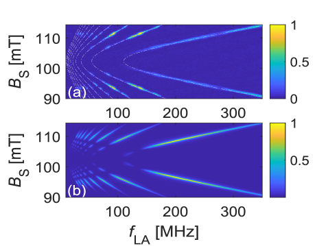
Figure 3: ODMR with low laser power. (a) The normalized ODMR signal as a function of driving frequency $f_{\mathrm{LA}}$ and magnetic field $B_{\mathrm{S}}$. The overlaid hyperbolas are calculated according to Eq. (3). (b) The normalized steady state polarization $P_{z}/P_{z,\mathrm{s}}$ is calculated according the Eq. (4) with the following parameters $\omega_{\mathrm{c}}=2\pi\times 276\operatorname{MHz}$, $\gamma_{\mathrm{c}}=2.87\operatorname{MHz}$, $\gamma_{1}=20\operatorname{Hz}$ and $\gamma_{2}=30\operatorname{MHz}$. In terms of the parameter $\eta$ the coupling coefficient $\beta_{\Delta}$ is expressed as $\beta_{\Delta}=\beta_{\Delta 0}\eta/\sqrt{1+\eta^{2}}$, where $\beta_{\Delta 0}=10$.

IV Cavity Superharmonic Resonances

The effect of the coupled cavity mode on the spin MPR is discussed in Appendix A. The theoretical model presented in the appendix describes the interplay between two mechanisms. The first one is frequency mixing between transverse and longitudinal spin driving. Near the avoided crossing point the NV^- spin states with magnetic quantum numbers $-1$ and $0$ are mixed, and consequently the amplitudes of transverse and longitudinal driving become strongly dependent on detuning from the avoided crossing point (even when the external driving is kept unchanged). The highly nonlinear nature of the first mechanism results in the generation of harmonics of the externally applied driving frequency. The second mechanism is cavity resonance enhancement, which becomes efficient when one of the generated harmonics coincides with the cavity resonance band. Under appropriate conditions this may give rise to a pronounce cavity-assisted multi-photon resonance.

Consider the case where the frequency of excitation injected into the loop antenna is tuned close to the $l$’th superharmonic resonance, i.e. $\omega_{\mathrm{a}}\simeq l\omega_{\mathrm{LA}}$, where $l$ is an integer. In that region, the relative change $P_{z}/P_{z,\mathrm{s}}$ in spin polarization in the NV^- triplet ground state is found to be given by [see Eq. (39) in appendix A]

$$\frac{P_{z}}{P_{z,\mathrm{s}}}=1-\frac{\beta_{\Delta}^{2}\left|\zeta\right|^{2}}{1+\beta_{\Delta}^{2}\left|\zeta\right|^{2}+\beta_{\mathrm{a}l}^{2}}\;,$$ (4)

where [see Eq. (49)]

$$\zeta=J_{l}\left(\frac{\omega_{\mathrm{b}}}{\omega_{\mathrm{L}}}\right)\left(1+\frac{\kappa J_{0}^{2}\left(\frac{\omega_{\mathrm{b}}}{\omega_{\mathrm{L}}}\right)P_{z,\mathrm{s}}}{\left(1+i\beta_{\mathrm{c}l}\right)\left(1+i\beta_{\mathrm{a}l}\right)}\right)\;,$$ (5)

$\omega_{\mathrm{b}}$ is the amplitude of longitudinal spin driving [see Eq. (14)], the dimensionless coupling coefficient $\beta_{\Delta}$ is given by $\beta_{\Delta}=\omega_{\Delta}/\sqrt{\gamma_{1}\gamma_{2}}$, the dimensionless detuning coefficients $\beta_{\mathrm{c}l}$ and $\beta_{\mathrm{a}l}$ are given by $\beta_{\mathrm{c}l}=\left(\omega_{\mathrm{c}}-l\omega_{\mathrm{LA}}\right)/\gamma_{\mathrm{c}}$ and $\beta_{\mathrm{a}l}=\left(\omega_{\mathrm{a}}-l\omega_{\mathrm{LA}}\right)/\gamma_{2}$, respectively, $\omega_{\mathrm{c}}$ is the cavity mode angular frequency, $\gamma_{\mathrm{c}}$ is the cavity mode damping rate, $\gamma_{1}$ and $\gamma_{2}$ are the longitudinal and transverse spin damping rates, respectively and $\kappa=g^{2}/\gamma_{2}\gamma_{\mathrm{c}}$ is the cooperativity parameter. A plot of the normalized steady state polarization $P_{z}/P_{z,\mathrm{s}}$ given by Eq. (4) is shown in Fig. 3(b). The comparison between data and theory yields a qualitative agreement.

V P1

ODMR data near the LAC with relatively high laser power is shown in Fig. 4. The increase in laser power gives rise to excessive heating, and consequently the superconducting resonator mode becomes undetectable (in a microwave reflectivity measurement) due to a super to normal conduction phase transition of the spiral. The plot contains a variety of peaks all occurring along the above discussed hyperbolas [see Eq. (3)], suggesting that some multiphoton processes continue to exist regardless of the spiral resonator state. Locations of all data peaks are determined by a single frequency denoted by $f_{\mathrm{m}}$. This can be seen from the cross symbols added to Fig. 4. The frequency $f_{k,l}$ of the $k$’th cross symbol overlaid on the $l$’th hyperbola in Fig. 4 is given by

$$f_{k,l}=\frac{k}{l}f_{\mathrm{m}}\;,$$ (6)

where the frequency $f_{\mathrm{m}}$ takes the value $f_{\mathrm{m}}=86\operatorname{MHz}$. This pattern of peaks remains visible with the same value of $f_{\mathrm{m}}$ over a wide range of input microwave power (between $10$ and $25\operatorname{dBm}$), tenfold laser power attenuation, a few degrees magnetic field misalignments and temperature change. With temperature rising to $30\operatorname{K}$, the signal from the higher order hyperbolas disappears, but the $f_{\mathrm{m}}$ beating remains on the main hyperbola. The fact that some of the peaks do not appear at the same frequency for different magnetic fields validates that the pattern is not a measurement artifact of spurious resonances. In addition, the synthesizer signal harmonics were carefully examined with a spectrum analyzer to verify they are all well below the ODMR sensitivity threshold. The measured value of $f_{\mathrm{m}}$ suggests a connection between MPR in the NV^- defects and P1 defect Smith et al. (1959); Cook and Whiffen (1966); Loubser and van Wyk (1978); Barklie and Guven (1981), as is discussed below.

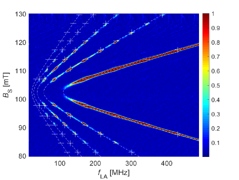
Figure 4: ODMR with high laser power. The overlaid hyperbolas are calculated according to Eq. (3) and the locations of the cross symbols according to Eq. (6).

P1 defect has four locally stable configurations. In each configuration a static Jahn-Teller distortion occurs, and an unpaired electron is shared by the nitrogen atom and by one of the four neighboring carbon atoms, which are positioned along one of the lattice directions $\left[111\right]$, $\left[\bar{1}11\right]$, $\left[1\bar{1}1\right]$ or $\left[11\bar{1}\right]$ Takahashi et al. (2008); Hanson et al. (2008); Wang et al. (2014); Broadway et al. (2016); Shim et al. (2013); Smeltzer et al. (2011); Shin et al. (2014); Clevenson et al. (2016); Schuster et al. (2010).

When both nuclear Zeeman shift and nuclear quadrupole coupling are disregarded, the spin Hamiltonian of a P1 defect is given by Loubser and van Wyk (1978); Schuster et al. (2010); Wood et al. (2016) $\mathcal{H}=\gamma_{\mathrm{e}}\mathbf{B}\cdot\mathbf{S}+\hbar^{-1}A_{\perp}\left(S_{x}I_{x}+S_{y}I_{y}\right)+\hbar^{-1}A_{\parallel}S_{z}I_{z}$, where $\mathbf{S}=\left(S_{x},S_{y},S_{z}\right)$ is an electronic spin 1/2 vector operator, $\mathbf{I}=\left(I_{x},I_{y},I_{z}\right)$ is a nuclear spin 1 vector operator, $A_{\parallel}=2\pi\times 114.03\operatorname{MHz}$ and $A_{\perp}=2\pi\times 81.33\operatorname{MHz}$ are respectively the longitudinal and transverse hyperfine parameters, and the $z$ direction corresponds to the diamond $\left\langle 111\right\rangle$ axis. The electron spin resonance at angular frequency $\gamma_{\mathrm{e}}B$ is split due to the interaction with the nuclear spin into three resonances, corresponding to three transitions, in which the nuclear spin magnetic quantum number is conserved Slichter (2013); Simanovskaia et al. (2013); Belthangady et al. (2013); van Oort et al. (1990); Hanson et al. (2008); Hall et al. (2016). For a magnetic field larger than a few $\operatorname{mT}$ the angular resonance frequencies are approximately given by $\gamma_{\mathrm{e}}B$ and $\gamma_{\mathrm{e}}B\pm\omega_{\mathrm{en}}$, where $\omega_{\mathrm{en}}^{2}=A_{\parallel}^{2}\cos^{2}\theta_{\mathrm{B}}+A_{\perp}^{2}\sin^{2}\theta_{\mathrm{B}}$ and where $\theta_{\mathrm{B}}$ is the angle between the magnetic field $\mathbf{B}$ and the P1 axis Smith et al. (1959).

Consider the case where $\mathbf{B}$ is in the lattice direction $\left[111\right]$. For this case, for 1/4 of the P1 defects $\omega_{\mathrm{en}}=2\pi\times 114\operatorname{MHz}$, whereas for the other 3/4 of the P1 defects [unparallel to $\mathbf{B}$ having axis in one of the lattice directions $\left[\bar{1}11\right]$, $\left[1\bar{1}1\right]$ or $\left[11\bar{1}\right]$] $\omega_{\mathrm{en}}=2\pi\times 85.6\operatorname{MHz}$, close to the observed value of the frequency $f_{\mathrm{m}}=86\operatorname{MHz}$. The fact that the parallel P1 defects do not have a significant effect on the ODMR data can be attributed to the fact that these defects generate only transverse driving for the NV^- defects having axis parallel to the crystal direction $\left[111\right]$, whereas the unparallel P1 defects generate both transverse and longitudinal driving, which in turn allows nonlinear processes of frequency mixing Cohen-Tannoudji et al. (1998).

The effect of dipolar interactions on the measured ODMR signal can be estimated using perturbation theory. To first order the above-discussed hyperfine splitting has no effect. However, as is argued below, a non-vanishing effect is obtained from the second order. Consider a pair of P1 defects with a dipolar coupling to a single NV^- defect Hanson et al. (2006); Bermudez et al. (2011); Kohl et al. (1988); Cheng (1961); Daycock and Jones (1969); Alekseev (1975); Varada and Agarwal (1992). Both P1 defects are assumed to be unparallel to $\mathbf{B}$, i.e. the frequencies of their electronic-like transitions are approximately given by $\gamma_{\mathrm{e}}B/2\pi$ and $\gamma_{\mathrm{e}}B/2\pi\pm 85.6\operatorname{MHz}$. The NV^- defect, on the other hand, is assumed to be nearly parallel to $\mathbf{B}$, thus having an energy separation of $2\hbar\gamma_{\mathrm{e}}B$ between the spin states with magnetic number $\pm 1$.

OISP polarizes the NV^- to the $m_{\mathrm{s}}=0$ state. The required condition for ODMR signal along the $l$-th hyperbola is achieved by excitation at $\omega_{\mathrm{LA}}=\omega_{\mathrm{a}}/l$, populating the $m_{\mathrm{s}}=-1$ state, which has lower photoluminescence. Let $(m_{\mathrm{S}}^{\mathrm{NV}},m_{\mathrm{S}}^{\mathrm{P1a}}+m_{\mathrm{S}}^{\mathrm{P1b}},m_{\mathrm{I}}^{\mathrm{P1a}}+m_{\mathrm{I}}^{\mathrm{P1b}})$ designate a subspace, where $m_{\mathrm{S}}^{\mathrm{NV}}$ is the NV^- electronic spin magnetic number, $m_{\mathrm{S}}^{\mathrm{P1a}}$ ($m_{\mathrm{S}}^{\mathrm{P1b}}$) is the first (second) P1 electronic spin magnetic number and $m_{\mathrm{I}}^{\mathrm{P1a}}$ ($m_{\mathrm{I}}^{\mathrm{P1b}}$) is the first (second) P1 nuclear spin magnetic number. Note that subspaces $(-1,+1,j)$ and $(+1,-1,j)$ for $j\in\{-2,-1,0,1,2\}$, are energetically separated by $\hbar|j|\omega_{\mathrm{en}}$. When $\omega_{\mathrm{a}}=k\omega_{\mathrm{en}}$ for integer $k$, transitions are stimulated between $(-1,+1,j)$ and $(+1,-1,j)$, further reducing the population of $(0,+1,j)$ and consequently enhancing the ODMR signal.

By employing perturbation theory Schrieffer and Wolff (1966) we find that the effective Rabi rate for these tripolar transitions is roughly given by $\omega_{\mathrm{P1P1NV}}\simeq\left(n_{\mathrm{S},\mathrm{P1}}/n_{\mathrm{D}}\right)^{2}D$, where $n_{\mathrm{S},\mathrm{P1}}$ is the density of P1 defects (which is assumed to be about $100$ times larger than the density of NV^- defects, and which can be expressed in terms of the relative concentration of nitrogen atoms $p_{\mathrm{N}}$ as $n_{\mathrm{S},\mathrm{P1}}=1.8\times 10^{23}\operatorname{cm}^{-3}p_{\mathrm{N}}$) and where $n_{\mathrm{D}}=4\pi D/\mu_{0}\gamma_{\mathrm{e}}^{2}\hbar=5.5\times 10^{22}\operatorname{cm}^{-3}$. The roughly estimated value of $p_{\mathrm{N}}=10^{-4}$ yields the rate $\omega_{\mathrm{P1P1NV}}/2\pi\simeq 300\operatorname{Hz}$. In a similar setup Alfasi et al. (2019), at $T=3.5\operatorname{K}$ the maximal OISP rate was found to be $T_{\mathrm{1O}}^{-1}\approx 200\operatorname{Hz}$ and $\gamma_{1}\approx 25\operatorname{Hz}$, hence this mechanism is expected to be of significance to a low temperature ODMR measurement.

Note that the transition between $(-1,+1,0)$ and $(+1,-1,0)$ does not require additional energy. Stimulated nuclear spin rotation with $\omega_{\mathrm{a}}=k\omega_{\mathrm{en}}/2$ for integer $k$ allows population of $(+1,-1,j_{1})$ for $j_{1}\in\{-2,-1,1,2\}$ via processes of sequential photons absorption. This effect gives rise to the weak peaks on the second ($l=2$) hyperbola in Fig. 4.

The MPR can be employed for enhancing the responsivity of diamond based magnetometry. Consider a setup with small frequency modulation about a central frequency $f_{\textmd{LA}}$ and photoluminescence signal $I$ demodulation readout. To maximize the responsivity, the bias magnetic field $B_{\textmd{S}}$ and $f_{\textmd{LA}}$ should be set to maximize the derivative $|\mathrm{d}I/\mathrm{d}f_{\textmd{LA}}|$. As can be seen in Fig. 5, $|\mathrm{d}I/\mathrm{d}f_{\textmd{LA}}|$ is maximal near the spots associated with P1 hyperfine transitions at the MPR of NV. This enhancement is attributed to the relatively narrow resonance of the P1 process as compared to the NV MPR.

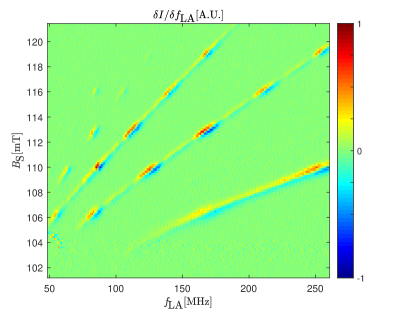
Figure 5: Derivative of the ODMR photoluminescence signal $I$ with respect to the driving signal frequency $f_{\textmd{LA}}$ at high laser power. The absolute maximal values are achieved not along the single photon curve (bottom right diagonal), but rather at the spots attributed to P1 hyperfine processes on the NV MPR curves (top left diagonals).

VI Summary

Multiphoton processes are surprisingly well measurable in Ib diamonds, making this mode of operation preferable for enhanced sensitivity in multiple applications. Of particular interest is the interaction of the optically measurable and polarizable NV ensemble with the naturally occurring P1 ensemble. The unexpected strength of coupling to the hyperfine transitions of the P1 requires further investigation to determine the nature of the interaction. The NV defects can potentially provide an optical access to a much denser and coherent (nuclear) ensemble of the P1.

VII Acknowledgements

We greatly appreciate fruitful discussions with Paz London, Aharon Blank, Efrat Lifshitz, Vladimir Dyakonov, Sergey Tarasenko, Victor Soltamov, Nadav Katz, Michael Stern and Nir Bar-Gil.

Appendix A Driven Spins Coupled to a Resonator

Consider a cavity mode coupled to a spin ensemble. The Hamiltonian of the closed system is taken to be given by

$$\hbar^{-1}\mathcal{H}_{0}=\omega_{\mathrm{c}}A^{{\dagger}}A+\frac{\mathbf{\Omega\cdot\Sigma}}{2}+g\left(A\Sigma_{+}+A^{{\dagger}}\Sigma_{-}\right)\ ,$$ (7)

where $\omega_{\mathrm{c}}$ is the cavity mode angular frequency, $A^{{\dagger}}A$ is a cavity mode number operator, $\mathbf{\Sigma}=\left(\Sigma_{x},\Sigma_{y},\Sigma_{z}\right)$, the spin operators $\Sigma_{z}$, $\Sigma_{+}=\left(\Sigma_{x}+i\Sigma_{y}\right)/2$ and $\Sigma_{-}=\left(\Sigma_{x}-i\Sigma_{y}\right)/2$ are related to the eigenvectors $\left|\pm\right\rangle$ of the operator $\Sigma_{z}$ by

$$\Sigma_{z} =\left|+\right\rangle\left\langle+\right|-\left|-\right\rangle\left\langle-\right|\;,$$ (8)

$$\Sigma_{+} =\left|+\right\rangle\left\langle-\right|\;,$$ (9)

$$\Sigma_{-} =\left|-\right\rangle\left\langle+\right|\;.$$ (10)

The effective magnetic field $\mathbf{\Omega}\left(t\right)$ is expressed in terms of the angular frequency $\omega_{\mathrm{T}}$ and amplitude $\omega_{1}$ of transverse driving, the longitudinal magnetic field component $\omega_{0}\left(t\right)$ and transverse one $\omega_{\Delta}$

$$\mathbf{\Omega}\left(t\right)=\omega_{1}\left(\cos\left(\omega_{\mathrm{T}}t\right)\mathbf{\hat{x}}+\sin\left(\omega_{\mathrm{T}}t\right)\mathbf{\hat{y}}\right)+\omega_{0}\mathbf{\hat{z}}+\omega_{\Delta}\mathbf{\hat{x}}\ ,$$ (11)

or

$$\mathbf{\Omega}\left(t\right) =\omega_{1}\left(e^{-i\omega_{\mathrm{T}}t}\mathbf{\hat{u}}_{+}+e^{i\omega_{\mathrm{T}}t}\mathbf{\hat{u}}_{-}\right)+\omega_{0}\left(t\right)\mathbf{\hat{z}}$$

$$+\omega_{\Delta}\left(\mathbf{\hat{u}}_{+}+\mathbf{\hat{u}}_{-}\right)\ ,$$

(12)

where $\omega_{\Delta}$ is a real constant and

$$\mathbf{\hat{u}}_{\pm}=\left(1/2\right)\left(\mathbf{\hat{x}}\pm i\mathbf{\hat{y}}\right)\ .$$ (13)

While $\omega_{1}$ and $\omega_{\mathrm{T}}$ are both assumed to be real constants, $\omega_{0}$ is allowed to vary in time according to

$$\omega_{0}=\omega_{\mathrm{a}}-\omega_{\mathrm{b}}\sin\left(\omega_{\mathrm{L}}t\right)\;,$$ (14)

where $\omega_{\mathrm{a}}$, $\omega_{\mathrm{b}}$ and $\omega_{\mathrm{L}}$ are all real constants.

The following Bose

$$\left[A,A^{\dagger}\right]=1\;,$$ (15)

and spin

$$\left[\Sigma_{z},\Sigma_{+}\right] =2\Sigma_{+}\;,$$ (16)

$$\left[\Sigma_{z},\Sigma_{-}\right] =-2\Sigma_{-}\;,$$ (17)

$$\left[\Sigma_{+},\Sigma_{-}\right] =\Sigma_{z}\;,$$ (18)

commutation relations are assumed to hold. The Heisenberg equations of motion are generated according to

$$\frac{\mathrm{d}O}{\mathrm{d}t}=-i\left[O,\hbar^{-1}\mathcal{H}_{0}\right]\;,$$ (19)

where $O$ is an operator, hence

$$\frac{\mathrm{d}A}{\mathrm{d}t}=-i\omega_{\mathrm{c}}A-ig\Sigma_{-}\;,$$ (20)

$$\frac{\mathrm{d}\Sigma_{z}}{\mathrm{d}t}=W_{1}\Sigma_{+}+W_{1}^{{\dagger}}\Sigma_{-}\;,$$ (21)

and

$$\frac{\mathrm{d}\Sigma_{+}}{\mathrm{d}t}=i\omega_{0}\Sigma_{+}-\frac{W_{1}^{{\dagger}}}{2}\Sigma_{z}\;,$$ (22)

where

$$W_{1}=-i\left(\omega_{1}e^{-i\omega_{\mathrm{T}}t}+\omega_{\Delta}+2gA\right)\;.$$ (23)

Averaging

$$\left\langle A\right\rangle =\alpha\;,$$ (24)

$$\left\langle\Sigma_{z}\right\rangle =P_{z}\;,$$ (25)

$$\left\langle\Sigma_{\pm}\right\rangle =P_{\pm}\;,$$ (26)

and introducing damping leads to

$$\frac{\mathrm{d}\alpha}{\mathrm{d}t}=-\left(i\omega_{\mathrm{c}}+\gamma_{\mathrm{c}}\right)\alpha-igP_{-}\;,$$ (27)

$$\frac{\mathrm{d}P_{z}}{\mathrm{d}t}=\Omega_{1}P_{+}+\Omega_{1}^{\ast}P_{-}-\gamma_{1}\left(P_{z}-P_{z,\mathrm{s}}\right)\;,$$ (28)

and

$$\frac{\mathrm{d}P_{+}}{\mathrm{d}t}=i\omega_{0}P_{+}-\frac{\Omega_{1}^{\ast}}{2}P_{z}-\gamma_{2}P_{+}\;,$$ (29)

where $\gamma_{\mathrm{c}}$ is the cavity mode damping rate, $\gamma_{1}$ and $\gamma_{2}$ are the longitudinal and transverse spin damping rates, respectively, and where

$$\Omega_{1}=-i\left(\omega_{1}e^{-i\omega_{\mathrm{T}}t}+\omega_{\Delta}+2g\alpha\right)\;.$$ (30)

For our experimental conditions the term proportional to $\omega_{1}$ in Eq. (30) can be disregarded.

The effect of OISP can be accounted for by adjusting the values of the longitudinal damping rate $\gamma_{1}$ and steady state polarization $P_{z,\mathrm{s}}$ and make them both dependent on laser intensity Shin et al. (2012); Alfasi et al. (2018). In this approach $\gamma_{1}$ is given by $\gamma_{1}=\gamma_{1\mathrm{T}}+\gamma_{1\mathrm{O}}$, where $\gamma_{1\mathrm{T}}$ is the rate of thermal relaxation and $\gamma_{1\mathrm{O}}$ is the rate of OISP (proportional to laser intensity), and the averaged value of steady state polarization $P_{z,\mathrm{s}}$ is given by

$$P_{z,\mathrm{s}}=\frac{\gamma_{1\mathrm{T}}P_{z,\mathrm{ST}}+\gamma_{1\mathrm{O}}P_{z,\mathrm{SO}}}{\gamma_{1}}\;.$$ (31)

While $P_{z,\mathrm{ST}}$ represents the steady state polarization in the limit $\gamma_{1\mathrm{T}}\gg\gamma_{1\mathrm{O}}$ (i.e. when OISP is negligibly small), the value is $P_{z,\mathrm{SO}}$ for the other extreme case of $\gamma_{1\mathrm{O}}\gg\gamma_{1\mathrm{T}}$ (i.e. when thermal relaxation is negligibly small).

By employing the transformation

$$P_{+}=e^{i\theta_{\mathrm{d}}}P_{\mathrm{d}+}\ ,$$ (32)

where

$$\theta_{\mathrm{d}}=\int\nolimits^{t}\mathrm{d}t^{\prime}\;\left[\omega_{0}\left(t^{\prime}\right)+\Delta\right]\;,$$ (33)

and where $\Delta$ is a real constant (to be determined later), Eqs. (27), (28) and (29) become

$$\frac{\mathrm{d}\alpha}{\mathrm{d}t}=-\left(i\omega_{\mathrm{c}}+\gamma_{\mathrm{c}}\right)\alpha-ig\left(\frac{\omega_{\Delta}\zeta}{\Omega_{1}}\right)^{\ast}P_{\mathrm{d}+}^{\ast}\;,$$ (34)

$$\frac{\mathrm{d}P_{z}}{\mathrm{d}t}=\omega_{\Delta}\left(\zeta P_{\mathrm{d}+}+\zeta^{\ast}P_{\mathrm{d}+}^{\ast}\right)-\gamma_{1}\left(P_{z}-P_{z,\mathrm{s}}\right)\;,$$ (35)

and

$$\frac{\mathrm{d}P_{\mathrm{d}+}}{\mathrm{d}t}=-i\Delta P_{\mathrm{d}+}-\frac{\omega_{\Delta}\zeta^{\ast}}{2}P_{z}-\gamma_{2}P_{\mathrm{d}+}\;,$$ (36)

where

$$\zeta=\frac{\Omega_{1}}{\omega_{\Delta}}e^{i\theta_{\mathrm{d}}}\;.$$ (37)

When $\zeta$ is treated as a constant the steady state solution of Eqs. (35) and (36) reads

$$P_{\mathrm{d}+}=\frac{\omega_{\Delta}\zeta^{\ast}P_{z}}{2\left(-i\Delta-\gamma_{2}\right)}\;,$$ (38)

and

$$\frac{P_{z}}{P_{z,\mathrm{s}}}=1-\frac{\frac{\left|\omega_{\Delta}\zeta\right|^{2}}{\gamma_{1}\gamma_{2}}}{1+\frac{\left|\omega_{\Delta}\zeta\right|^{2}}{\gamma_{1}\gamma_{2}}+\frac{\Delta^{2}}{\gamma_{2}^{2}}}\;.$$ (39)

With the help of the Jacobi-Anger expansion, which is given by

$$\exp\left(iz\cos\theta\right)=\sum\limits_{n=-\infty}^{\infty}i^{n}J_{n}\left(z\right)e^{in\theta}\;,$$ (40)

one obtains [see Eqs. (14) and (37)]

$$\zeta=\frac{\Omega_{1}}{\omega_{\Delta}}e^{-\frac{i\omega_{\mathrm{b}}}{\omega_{\mathrm{L}}}}\sum\limits_{l^{\prime}=-\infty}^{\infty}i^{l^{\prime}}J_{l^{\prime}}\left(\frac{\omega_{\mathrm{b}}}{\omega_{\mathrm{L}}}\right)e^{i\left(\omega_{\mathrm{a}}+\Delta+l^{\prime}\omega_{\mathrm{L}}\right)t}\;.$$ (41)

Consider the case where $\omega_{\mathrm{a}}\simeq l\omega_{\mathrm{L}}$, where $l$ is an integer. For this case the detuning $\Delta$ is chosen to be given by $\Delta=l\omega_{\mathrm{L}}-\omega_{\mathrm{a}}$, and consequently $\zeta$ becomes

$$\zeta=\frac{\Omega_{1}}{\omega_{\Delta}}e^{-\frac{i\omega_{\mathrm{b}}}{\omega_{\mathrm{L}}}}\sum\limits_{l^{\prime}=-\infty}^{\infty}i^{l^{\prime}}J_{l^{\prime}}\left(\frac{\omega_{\mathrm{b}}}{\omega_{\mathrm{L}}}\right)e^{i\left(l+l^{\prime}\right)\omega_{\mathrm{L}}t}\;.$$ (42)

The driving term of Eq. (34) $-ig\left(\omega_{\Delta}\zeta/\Omega_{1}\right)^{\ast}P_{\mathrm{d}+}^{\ast}$ is approximated by keeping only the term $l^{\prime}=0$ in Eq. (42). When $P_{\mathrm{d}+}^{\ast}$ is treated as a constant Eq. (34) yields a steady state solution given by $\alpha=\alpha_{0}e^{-il\omega_{\mathrm{L}}t}$, where

$$\alpha_{0}=-\frac{ige^{\frac{i\omega_{\mathrm{b}}}{\omega_{\mathrm{L}}}}J_{0}\left(\frac{\omega_{\mathrm{b}}}{\omega_{\mathrm{L}}}\right)P_{\mathrm{d}+}^{\ast}}{\gamma_{\mathrm{c}}\left(1+i\beta_{\mathrm{c}l}\right)}\;,$$ (43)

and where

$$\beta_{\mathrm{c}l}=\frac{\omega_{\mathrm{c}}-l\omega_{\mathrm{L}}}{\gamma_{\mathrm{c}}}\;.$$ (44)

To lowest non vanishing order in the coupling $g$ the coefficient $P_{\mathrm{d}+}^{\ast}$ in Eq. (43) is evaluated using Eq. (38) by keeping only the term $l^{\prime}=-l$ in Eq. (42) and keeping only the term $-i\omega_{\Delta}$ in Eq. (30)

$$P_{\mathrm{d}+}^{\ast}=\frac{i^{1-l}e^{-\frac{i\omega_{\mathrm{b}}}{\omega_{\mathrm{L}}}}\omega_{\Delta}J_{-l}\left(\frac{\omega_{\mathrm{b}}}{\omega_{\mathrm{L}}}\right)P_{z,\mathrm{s}}}{2\gamma_{2}\left(1+i\beta_{\mathrm{a}l}\right)}\;,$$ (45)

where

$$\beta_{\mathrm{a}l}=\frac{\omega_{\mathrm{a}}-l\omega_{\mathrm{L}}}{\gamma_{2}}\;,$$ (46)

and thus [see Eq. (43)]

$$\alpha_{0}=-\frac{i^{2-l}g\omega_{\Delta}}{\gamma_{\mathrm{c}}\gamma_{2}}\frac{J_{0}\left(\frac{\omega_{\mathrm{b}}}{\omega_{\mathrm{L}}}\right)J_{-l}\left(\frac{\omega_{\mathrm{b}}}{\omega_{\mathrm{L}}}\right)P_{z,\mathrm{s}}}{2\left(1+i\beta_{\mathrm{c}l}\right)\left(1+i\beta_{\mathrm{a}l}\right)}\;.$$ (47)

It is assumed that the dominant contribution of $\zeta$ to the equation of motion (35) and (36) comes from a term, which is labelled as $\zeta_{\mathrm{a}}$, which is given by [see Eqs. (30) and (42)]

$$ie^{\frac{i\omega_{\mathrm{b}}}{\omega_{\mathrm{L}}}}\zeta_{\mathrm{a}}=i^{-l}J_{-l}\left(\frac{\omega_{\mathrm{b}}}{\omega_{\mathrm{L}}}\right)+\frac{2g\alpha_{0}}{\omega_{\Delta}}J_{0}\left(\frac{\omega_{\mathrm{b}}}{\omega_{\mathrm{L}}}\right)\;.$$ (48)

With the help of Eq. (47) this becomes

$$i^{1+l}e^{\frac{i\omega_{\mathrm{b}}}{\omega_{\mathrm{L}}}}\zeta_{\mathrm{a}}=J_{-l}\left(\frac{\omega_{\mathrm{b}}}{\omega_{\mathrm{L}}}\right)\left(1+\frac{\kappa J_{0}^{2}\left(\frac{\omega_{\mathrm{b}}}{\omega_{\mathrm{L}}}\right)P_{z,\mathrm{s}}}{\left(1+i\beta_{\mathrm{c}l}\right)\left(1+i\beta_{\mathrm{a}l}\right)}\right)\;,$$ (49)

where the cooperativity parameter $\kappa$ is given by

$$\kappa=\frac{g^{2}}{\gamma_{2}\gamma_{\mathrm{c}}}\;.$$ (50)

The above results (39) and (49) lead to Eq. (4) in main text for the steady state polarization.

References

- Shirley (1965) J. H. Shirley, Physical Review 138, B979 (1965).
- Berns et al. (2006) D. M. Berns, W. D. Oliver, S. O. Valenzuela, A. V. Shytov, K. K. Berggren, L. S. Levitov, and T. P. Orlando, Physical Review Letters 97, 150502 (pages 4) (2006).
- Tycko and Opella (1987) R. Tycko and S. Opella, The Journal of chemical physics 86, 1761 (1987).
- Faisal (2013) F. H. Faisal, Theory of multiphoton processes (Springer Science & Business Media, 2013).
- Childress and McIntyre (2010) L. Childress and J. McIntyre, Physical Review A 82, 033839 (2010).
- Chen et al. (2018) H. Chen, E. MacQuarrie, and G. Fuchs, Physical review letters 120, 167401 (2018).
- Mamin et al. (2014) H. Mamin, M. Sherwood, M. Kim, C. Rettner, K. Ohno, D. Awschalom, and D. Rugar, Physical review letters 113, 030803 (2014).
- Mollow (1973) B. Mollow, in Coherence and Quantum Optics (Springer, 1973), pp. 525–532.
- Freedhoff and Quang (1994) H. Freedhoff and T. Quang, Physical review letters 72, 474 (1994).
- WEBER (1959) J. WEBER, Rev. Mod. Phys. 31, 681 (1959).
- Armen and Mabuchi (2006) M. A. Armen and H. Mabuchi, Physical Review A 73, 063801 (2006).
- Grossmann et al. (1991) F. Grossmann, T. Dittrich, P. Jung, and P. Hänggi, Physical review letters 67, 516 (1991).
- Lignier et al. (2007) H. Lignier, C. Sias, D. Ciampini, Y. Singh, A. Zenesini, O. Morsch, and E. Arimondo, Physical review letters 99, 220403 (2007).
- Fuchs et al. (2009) G. Fuchs, V. Dobrovitski, D. Toyli, F. Heremans, and D. Awschalom, Science p. 1181193 (2009).
- Doherty et al. (2013) M. W. Doherty, N. B. Manson, P. Delaney, F. Jelezko, J. Wrachtrup, and L. C. Hollenberg, Physics Reports 528, 1 (2013).
- Zhu et al. (2011) X. Zhu, S. Saito, A. Kemp, K. Kakuyanagi, S.-i. Karimoto, H. Nakano, W. J. Munro, Y. Tokura, M. S. Everitt, K. Nemoto, et al., Nature 478, 221 (2011).
- Kubo et al. (2010) Y. Kubo, F. Ong, P. Bertet, D. Vion, V. Jacques, D. Zheng, A. Dréau, J.-F. Roch, A. Auffèves, F. Jelezko, et al., Physical review letters 105, 140502 (2010).
- Kubo et al. (2011) Y. Kubo, C. Grezes, A. Dewes, T. Umeda, J. Isoya, H. Sumiya, N. Morishita, H. Abe, S. Onoda, T. Ohshima, et al., Physical review letters 107, 220501 (2011).
- Amsüss et al. (2011) R. Amsüss, C. Koller, T. Nöbauer, S. Putz, S. Rotter, K. Sandner, S. Schneider, M. Schramböck, G. Steinhauser, H. Ritsch, et al., Phys. Rev. Lett. 107, 060502 (2011).
- Schuster et al. (2010) D. Schuster, A. Sears, E. Ginossar, L. DiCarlo, L. Frunzio, J. Morton, H. Wu, G. Briggs, B. Buckley, D. Awschalom, et al., Physical review letters 105, 140501 (2010).
- Sandner et al. (2012) K. Sandner, H. Ritsch, R. Amsüss, C. Koller, T. Nöbauer, S. Putz, J. Schmiedmayer, and J. Majer, Physical Review A 85, 053806 (2012).
- Grezes et al. (2014) C. Grezes, B. Julsgaard, Y. Kubo, M. Stern, T. Umeda, J. Isoya, H. Sumiya, H. Abe, S. Onoda, T. Ohshima, et al., Physical Review X 4, 021049 (2014).
- Alfasi et al. (2018) N. Alfasi, S. Masis, R. Winik, D. Farfurnik, O. Shtempluck, N. Bar-Gill, and E. Buks, Physical Review A 97, 063808 (2018).
- Álvarez et al. (2015) G. A. Álvarez, C. O. Bretschneider, R. Fischer, P. London, H. Kanda, S. Onoda, J. Isoya, D. Gershoni, and L. Frydman, Nature communications 6, 8456 (2015).
- Kamp et al. (2018) E. Kamp, B. Carvajal, and N. Samarth, Physical Review B 97, 045204 (2018).
- Sushkov et al. (2014) A. Sushkov, I. Lovchinsky, N. Chisholm, R. L. Walsworth, H. Park, and M. D. Lukin, Physical review letters 113, 197601 (2014).
- Belthangady et al. (2013) C. Belthangady, N. Bar-Gill, L. M. Pham, K. Arai, D. Le Sage, P. Cappellaro, and R. L. Walsworth, Physical review letters 110, 157601 (2013).
- Doherty et al. (2012) M. Doherty, F. Dolde, H. Fedder, F. Jelezko, J. Wrachtrup, N. Manson, and L. Hollenberg, Physical Review B 85, 205203 (2012).
- Balasubramanian et al. (2009) G. Balasubramanian, P. Neumann, D. Twitchen, M. Markham, R. Kolesov, N. Mizuochi, J. Isoya, J. Achard, J. Beck, J. Tissler, et al., Nature materials 8, 383 (2009).
- Robledo et al. (2011) L. Robledo, H. Bernien, T. van der Sar, and R. Hanson, New Journal of Physics 13, 025013 (2011).
- Redman et al. (1991) D. Redman, S. Brown, R. Sands, and S. Rand, Physical review letters 67, 3420 (1991).
- Shin et al. (2012) C. S. Shin, C. E. Avalos, M. C. Butler, D. R. Trease, S. J. Seltzer, J. P. Mustonen, D. J. Kennedy, V. M. Acosta, D. Budker, A. Pines, et al., Journal of Applied Physics 112, 124519 (2012).
- Chapman and Plakhotnik (2011) R. Chapman and T. Plakhotnik, Chemical Physics Letters 507, 190 (2011).
- Gruber et al. (1997) A. Gruber, A. Dräbenstedt, C. Tietz, L. Fleury, J. Wrachtrup, and C. Von Borczyskowski, Science 276, 2012 (1997).
- Maze et al. (2008) J. Maze, P. Stanwix, J. Hodges, S. Hong, J. Taylor, P. Cappellaro, L. Jiang, M. G. Dutt, E. Togan, A. Zibrov, et al., Nature 455, 644 (2008).
- Acosta et al. (2010) V. Acosta, E. Bauch, M. Ledbetter, A. Waxman, L.-S. Bouchard, and D. Budker, Physical review letters 104, 070801 (2010).
- Balasubramanian et al. (2008) G. Balasubramanian, I. Chan, R. Kolesov, M. Al-Hmoud, J. Tisler, C. Shin, C. Kim, A. Wojcik, P. R. Hemmer, A. Krueger, et al., Nature 455, 648 (2008).
- Wolf et al. (2015) T. Wolf, P. Neumann, K. Nakamura, H. Sumiya, T. Ohshima, J. Isoya, and J. Wrachtrup, Physical Review X 5, 041001 (2015).
- Mamin et al. (2013) H. Mamin, M. Kim, M. Sherwood, C. Rettner, K. Ohno, D. Awschalom, and D. Rugar, Science 339, 557 (2013).
- Pelliccione et al. (2016) M. Pelliccione, A. Jenkins, P. Ovartchaiyapong, C. Reetz, E. Emmanouilidou, N. Ni, and A. C. B. Jayich, Nature nanotechnology 11, 700 (2016).
- Rondin et al. (2013) L. Rondin, J.-P. Tetienne, S. Rohart, A. Thiaville, T. Hingant, P. Spinicelli, J.-F. Roch, and V. Jacques, Nature communications 4, 2279 (2013).
- Dolde et al. (2011) F. Dolde, H. Fedder, M. W. Doherty, T. Nöbauer, F. Rempp, G. Balasubramanian, T. Wolf, F. Reinhard, L. Hollenberg, F. Jelezko, et al., Nature Physics 7, 459 (2011).
- Jelezko et al. (2004) F. Jelezko, T. Gaebel, I. Popa, A. Gruber, and J. Wrachtrup, Physical review letters 92, 076401 (2004).
- Maurer et al. (2012) P. C. Maurer, G. Kucsko, C. Latta, L. Jiang, N. Y. Yao, S. D. Bennett, F. Pastawski, D. Hunger, N. Chisholm, M. Markham, et al., Science 336, 1283 (2012).
- Cai et al. (2012) J. Cai, F. Jelezko, N. Katz, A. Retzker, and M. B. Plenio, New Journal of Physics 14, 093030 (2012).
- Takahashi et al. (2008) S. Takahashi, R. Hanson, J. van Tol, M. S. Sherwin, and D. D. Awschalom, Physical review letters 101, 047601 (2008).
- Fischer et al. (2013a) R. Fischer, C. O. Bretschneider, P. London, D. Budker, D. Gershoni, and L. Frydman, Physical review letters 111, 057601 (2013a).
- Fischer et al. (2013b) R. Fischer, A. Jarmola, P. Kehayias, and D. Budker, Physical Review B 87, 125207 (2013b).
- Wang et al. (2013) H.-J. Wang, C. S. Shin, C. E. Avalos, S. J. Seltzer, D. Budker, A. Pines, and V. S. Bajaj, Nature communications 4, 1940 (2013), article number: 1940.
- Solomon (1955) I. Solomon, Physical Review 99, 559 (1955).
- Loretz et al. (2017) M. Loretz, H. Takahashi, T. F. Segawa, J. M. Boss, and C. L. Degen, Physical Review B 95, 064413 (2017).
- Simanovskaia et al. (2013) M. Simanovskaia, K. Jensen, A. Jarmola, K. Aulenbacher, N. Manson, and D. Budker, Physical Review B 87, 224106 (2013).
- Clevenson et al. (2016) H. Clevenson, E. H. Chen, F. Dolde, C. Teale, D. Englund, and D. Braje, Phys. Rev. A 94, 021401 (2016).
- Wang et al. (2014) H.-J. Wang, C. S. Shin, S. J. Seltzer, C. E. Avalos, A. Pines, and V. S. Bajaj, Nature communications 5, 4135 (2014).
- Hall et al. (2016) L. Hall, P. Kehayias, D. Simpson, A. Jarmola, A. Stacey, D. Budker, and L. Hollenberg, Nature communications 7, 10211 (2016).
- Purser et al. (2018) C. M. Purser, V. P. Bhallamudi, C. S. Wolfe, H. Yusuf, B. A. McCullian, C. Jayaprakash, M. E. Flatté, and P. C. Hammel, arXiv:1802.09635 (2018).
- Alfasi et al. (2019) N. Alfasi, S. Masis, O. Shtempluck, and E. Buks, arXiv:1904.02911 [quant-ph] (2019).
- Kurter et al. (2011) C. Kurter, A. P. Zhuravel, J. Abrahams, C. L. Bennett, A. V. Ustinov, and S. M. Anlage, IEEE Transactions on Applied Superconductivity 21, 709 (2011).
- CST of America (2019) CST of America, Cst studio (2019).
- Ovartchaiyapong et al. (2014) P. Ovartchaiyapong, K. W. Lee, B. A. Myers, and A. C. B. Jayich, arXiv:1403.4173 (2014).
- MacQuarrie et al. (2013) E. MacQuarrie, T. Gosavi, N. Jungwirth, S. Bhave, and G. Fuchs, Physical review letters 111, 227602 (2013).
- Smith et al. (1959) W. Smith, P. Sorokin, I. Gelles, and G. Lasher, Physical Review 115, 1546 (1959).
- Cook and Whiffen (1966) R. Cook and D. Whiffen, Proceedings of the Royal Society of London A: Mathematical, Physical and Engineering Sciences 295, 99 (1966).
- Loubser and van Wyk (1978) J. Loubser and J. van Wyk, Reports on Progress in Physics 41, 1201 (1978).
- Barklie and Guven (1981) R. Barklie and J. Guven, Journal of Physics C: Solid State Physics 14, 3621 (1981).
- Hanson et al. (2008) R. Hanson, V. Dobrovitski, A. Feiguin, O. Gywat, and D. Awschalom, Science 320, 352 (2008).
- Broadway et al. (2016) D. A. Broadway, J. D. Wood, L. T. Hall, A. Stacey, M. Markham, D. A. Simpson, J.-P. Tetienne, and L. C. Hollenberg, arXiv:1607.04006 (2016).
- Shim et al. (2013) J. Shim, B. Nowak, I. Niemeyer, J. Zhang, F. Brandao, and D. Suter, arXiv:1307.0257 (2013).
- Smeltzer et al. (2011) B. Smeltzer, L. Childress, and A. Gali, New Journal of Physics 13, 025021 (2011).
- Shin et al. (2014) C. S. Shin, M. C. Butler, H.-J. Wang, C. E. Avalos, S. J. Seltzer, R.-B. Liu, A. Pines, and V. S. Bajaj, Physical Review B 89, 205202 (2014).
- Wood et al. (2016) J. D. Wood, D. A. Broadway, L. T. Hall, A. Stacey, D. A. Simpson, J.-P. Tetienne, and L. C. Hollenberg, Physical Review B 94, 155402 (2016).
- Slichter (2013) C. P. Slichter, Principles of magnetic resonance, vol. 1 (Springer Science & Business Media, 2013).
- van Oort et al. (1990) E. van Oort, P. Stroomer, and M. Glasbeek, Physical Review B 42, 8605 (1990).
- Cohen-Tannoudji et al. (1998) C. Cohen-Tannoudji, J. Dupont-Roc, and G. Grynberg, Atom-Photon Interactions: Basic Processes and Applications, by Claude Cohen-Tannoudji, Jacques Dupont-Roc, Gilbert Grynberg, pp. 678. ISBN 0-471-29336-9. Wiley-VCH, March 1998. p. 678 (1998).
- Hanson et al. (2006) R. Hanson, F. Mendoza, R. Epstein, and D. Awschalom, Physical review letters 97, 087601 (2006).
- Bermudez et al. (2011) A. Bermudez, F. Jelezko, M. Plenio, and A. Retzker, Physical review letters 107, 150503 (2011).
- Kohl et al. (1988) M. Kohl, M. Odehnal, V. Petříěek, R. Tichỳ, and S. Šafrata, Journal of low temperature physics 72, 319 (1988).
- Cheng (1961) H. Cheng, Phys. Rev. 124, 1359 (1961), URL https://link.aps.org/doi/10.1103/PhysRev.124.1359.
- Daycock and Jones (1969) J. Daycock and G. P. Jones, Journal of Physics C: Solid State Physics 2, 998 (1969).
- Alekseev (1975) B. Alekseev, Radiophysics and Quantum Electronics 18, 1272 (1975).
- Varada and Agarwal (1992) G. Varada and G. Agarwal, Physical Review A 45, 6721 (1992).
- Schrieffer and Wolff (1966) J. R. Schrieffer and P. A. Wolff, Phys. Rev. 149, 491 (1966).